
Fast Segmentation and Dynamic Monitoring of Time-Lapse 3D GPR Data Based on U-Net
by
 , and
, and
Ke Shang
1,2 ,
,
Feizhou Zhang
2, 
Ao Song
3,
Jianyu Ling
1,
Jiwen Xiao
4,
Zihan Zhang
2 and
Rongyi Qian
1,* 1
School of Geophysics and Information Technology, China University of Geosciences, Beijing 100083, China
2
School of Earth and Space Sciences, Peking University, Beijing 100871, China
3
National Institute of Natural Hazards, Ministry of Emergency Management of China (MEMC), Beijing 100085, China
4
Institute of Software Chinese Academy of Sciences, Beijing 100190, China
*
Author to whom correspondence should be addressed.
Remote Sens. 2022, 14(17), 4190; https://doi.org/10.3390/rs14174190
Submission received: 9 July 2022
/
Revised: 18 August 2022
/
Accepted: 24 August 2022
/
Published: 25 August 2022
(This article belongs to the Special Issue Road Extraction and Distress Assessment by Spaceborne, Airborne and Terrestrial Platforms)
Abstract
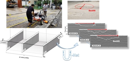
:As the amount of ground-penetrating radar (GPR) data increases significantly with the high demands of nondestructive detection methods under urban roads, a method suitable for time-lapse data dynamic monitoring should be developed to quickly identify targets on GPR profiles and compare time-lapse datasets. This study conducted a field experiment aiming to monitor one backfill pit using three-dimensional GPR (3D GPR), and the time-lapse data collected over four months were used to train U-Net, a fast neural network based on convolutional neural networks (CNNs). Consequently, a trained network model that could effectively segment the backfill pit from inline profiles was obtained, whose Intersection over Union (IoU) was 0.83 on the test dataset. Moreover, segmentation masks were compared, demonstrating that a change in the southwest side of the backfill pit may exist. The results demonstrate the potential of machine learning algorithms in time-lapse 3D GPR data segmentation and dynamic monitoring.
1. Introduction
Ground-penetrating radar (GPR) is a nondestructive detection technique that transmits high-frequency electromagnetic waves and receives the backscattering from the medium, which is suitable for defect inspection and dynamic monitoring of urban roads. To avoid road collapses, GPR is used to detect underground targets, including pipelines, voids, backfill pits, and high-water-cut areas. As it is known, it is not difficult to distinguish strong reflections from other signals, such as the reflections of metal pipes and clear boundaries of voids [1,2,3]. However, in many cases, the reason defects under roads are not discovered in time is that the radar data do not provide a strong reflection feature before the defect is generated, but cluttered weak scattering caused by loosening or deformation of the medium may be evident. Therefore, cases containing weak reflections with extended ranges should be approached seriously. Furthermore, to satisfy the goal of road safety maintenance, defects should be identified and monitored timely and properly to know if any changes occur or if actions are required to avoid road collapses. Identifying and locating regional features on GPR data are crucial and remain challenging tasks, because of the amplitude of the reflections as well as the regional characteristics that must be considered, which cannot be measured by mathematical formulas or specific values. In addition, the large amount of time-lapse data generated by GPR monitoring introduces difficulties in data processing and target identification. Therefore, the development of a method for the quick identification and monitoring of targets with regional features from time-lapse GPR data is necessary.
In recent years, convolutional neural networks (CNNs) and their neural network models have been widely applied in object recognition, image segmentation, and face and speech recognition owing to their powerful image processing abilities. Their advantage is that it is not necessary to know the quantitative characteristic parameters of the target; the network can learn the discriminant basis of the target from data from multiple trainings. In the user layer, this is represented as end-to-end mapping from the data to the target, hiding the complex judgment basis and quantitative criteria in the middle [4,5,6,7,8]. In recent years, CNNs have been used to identify hyperbolic features [9,10], manhole covers, reflective interfaces, soil [11,12], and landmines [13,14] in GPR data images. However, for defects in urban roads, research on object recognition and dynamic-change monitoring using machine learning is not comprehensive. Studies based on simulated data are insufficient, but the plausibility of real data must be discussed. In addition, both strongly and weakly reflected local signals should be considered, because any change in the data might indicate a change in the dielectric constant of the underground material. Therefore, with the necessity to identify specific obvious features and weak signals with regional characteristics, an appropriate neural network is required, which can achieve satisfactory recognition and segmentation results from limited GPR datasets.
U-Net is a deep learning network based on CNNs. Through powerful data augmentation, a reasonable weighted loss function, and full utilization of subunit neighborhood information, it can accurately identify image features with available annotated samples and realize end-to-end mappings between input data and segmentation units. Compared with other networks, it has the advantages of a simple structure, faster operation speed, and higher accuracy [15,16].
The main purpose of this study is to discuss a fast method for interpreting and comparing time-lapse GPR data in monitoring weak signal targets with regional characteristics. Firstly, the 3D GPR data acquisition and preprocessing methods are presented. Afterwards, the used neural network, U-Net, is presented along with how we used our data to train it. Finally, the detection results from the time-lapse dataset are compared and the results are discussed.
2. Experiment and Methods
2.1. Field Experiment and Data
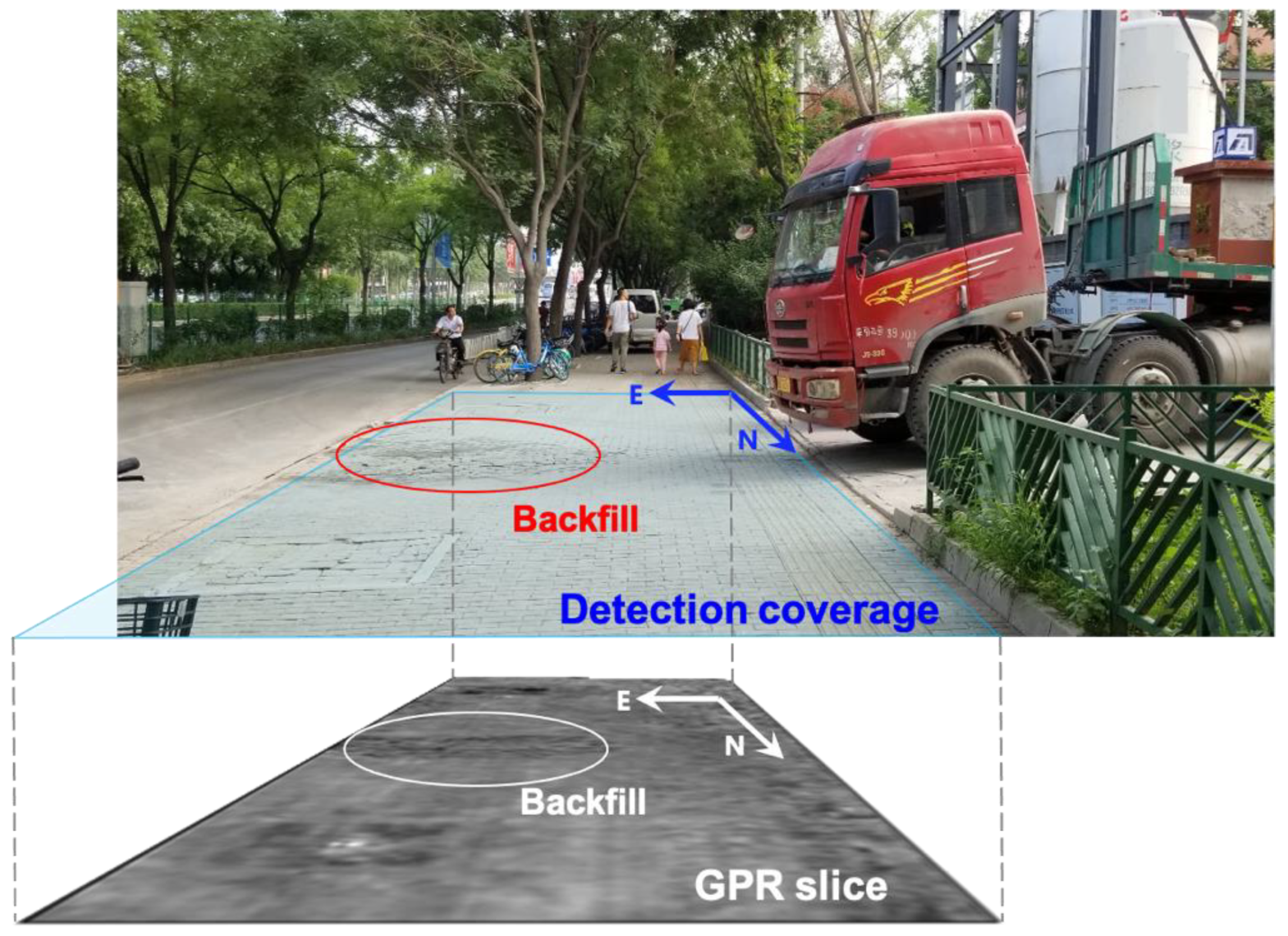
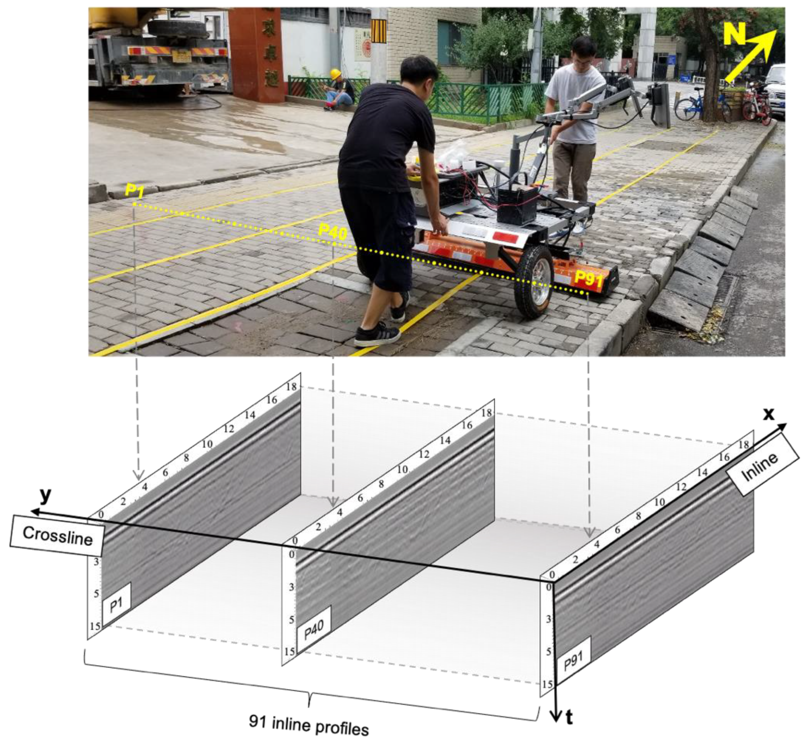
As shown in Figure 1, the experiment was conducted at the gate of a construction site with a fresh backfill pit. Considering the material in the backfill pit may be deformed after being crushed, a time-lapse full-coverage (TLFC) 3D GPR acquisition containing four group lines was arranged on the sidewalk, covering the backfill pit from inline profiles P40 to P91, as shown in Figure 2. The MobyScan-V 3D GPR system with the 30-channel antenna arrays (Figure 3) produced by DECOD Science & Technology Pte. Ltd. (Singapore). was used in this experiment, and Table 1 lists the acquisition parameters. Fifteen time-lapse detection sessions were conducted from 20 May to 25 October 2019 (Table A1).
The 3D data preprocessing methods listed in Table 2 were applied to the raw 3D GPR data, in which the first arrive disagreed with the true time zero, and useful reflection signals were buried by strong noise (Figure A1). Firstly, an antenna lifting test was carried out to find the position of the ground as the true zero, as shown in Figure A2. Then, time zero correction, background removal (BGR), and frequency filtering were applied in turn (Figure A3). Finally, correlation was used to carry out the 3D time zero normalization and 3D data combination, which can be found in Figure A4 and Figure A5 and [17]. The 3D GPR data cube after preprocessing is shown in Figure A6.
2.2. U-Net Structure and Model Training
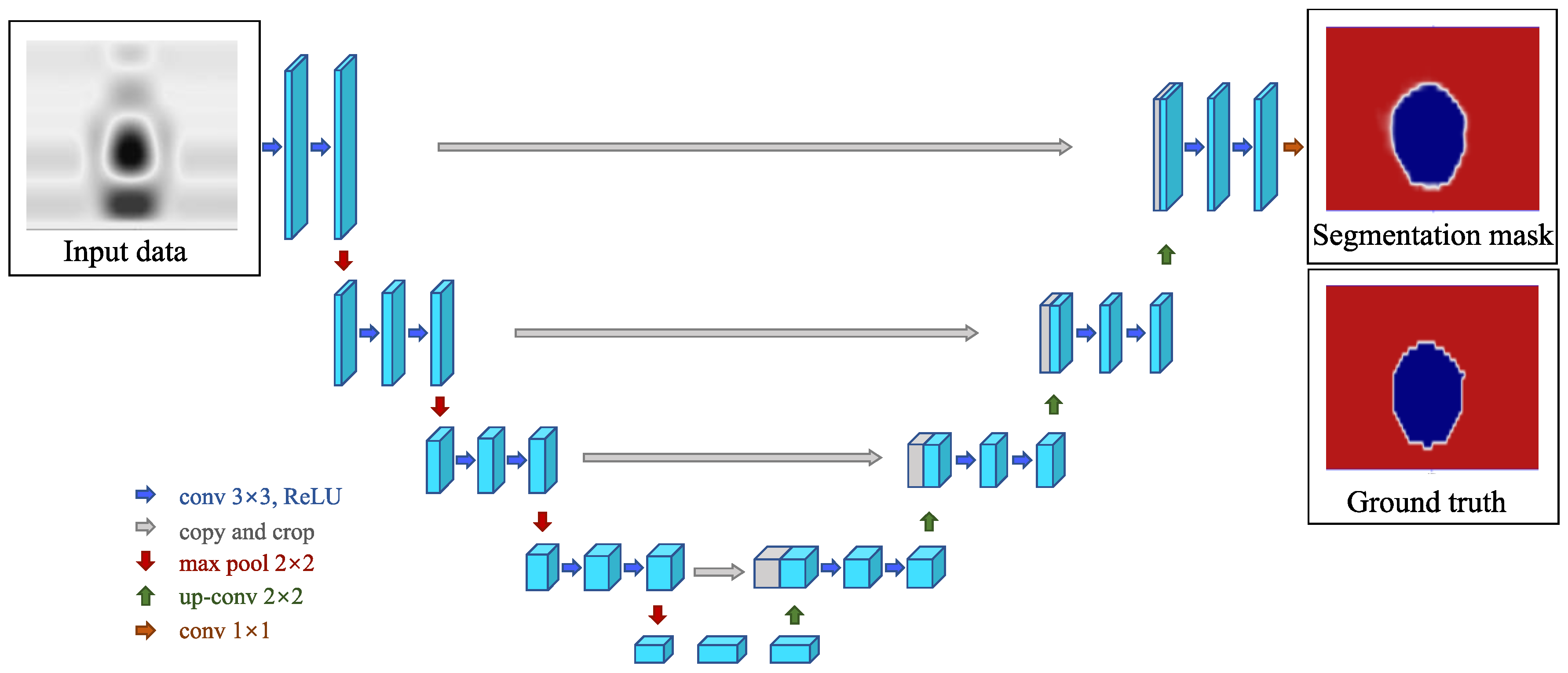
Figure 4 illustrates the U-Net architecture. The entire network presents a symmetrical “U” shape. It consists of contracting and expansive paths, which correspond to the left and right sides of the figure, respectively.
- Contracting path: This path is used to obtain the context information. It has four layers, and each layer consists of two identical 3 × 3 convolutions and rectified linear unit (ReLU) activation functions. Downsampling is performed through a 2 × 2 max pooling operation. The number of feature channels is doubled after each downsampling. On this path, four max pooling operations are performed to extract the feature information from the sample.
- Expansive path: This is the upsampling part used to locate the target. A 2 × 2 convolution is applied to half of the feature channels, and then two 3 × 3 convolutions are used, each followed by a ReLU function. In the last layer, a 1 × 1 convolution is used to map the feature vectors to the corresponding prediction classification to complete the data segmentation and make the size of the output data consistent with that of the input data.
2.3. Data Segmentation
For 3D GPR, data can be interpreted and annotated from different profiles, such as inline, crossline, and horizontal slices. In this study, the spatial resolution of inline profiles along the acquisition direction was higher. Therefore, the target areas in the inline profiles of the 3D GPR data were segmented pixel-wise to generate ground truths and show the clear borders of the target. These inline profiles with ground truths were used as the training and testing datasets.
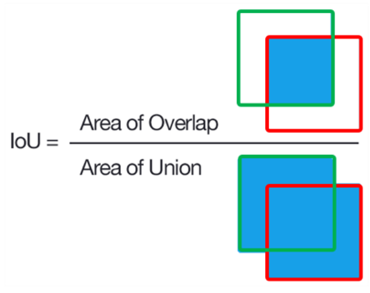
2.4. Accuracy Evaluation
The IoU between the segmentation and manual ground truth was applied to evaluate the network availability, as shown in Figure 5. The prediction results can be divided into the following two grades:
- , good result;
- , unsatisfactory result, and the segmentation is invalid.
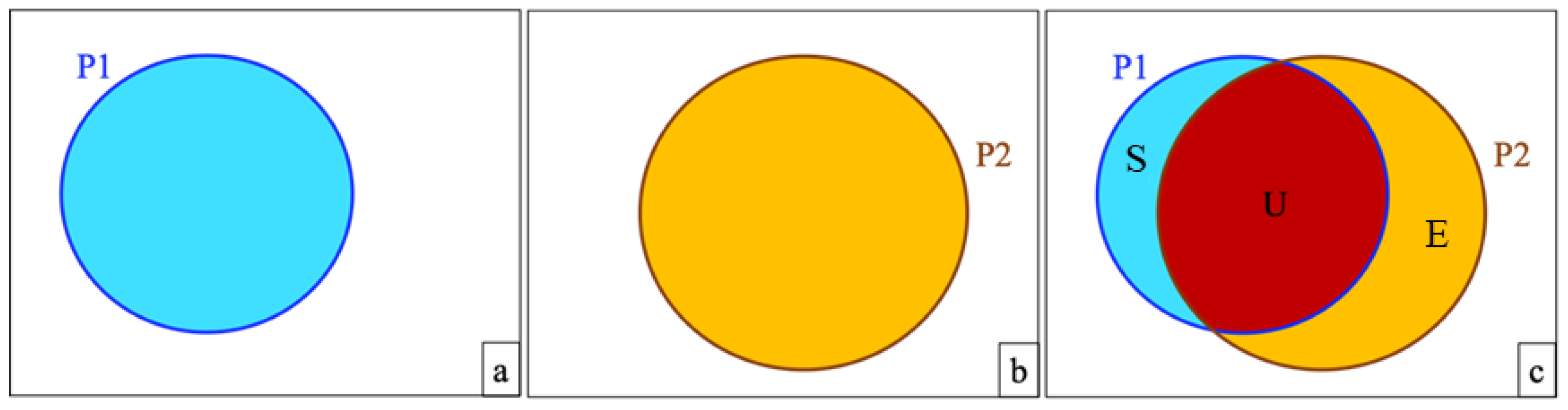
2.5. Mask Comparison
The changes in the targets can be determined by overlapping the masks of the time-lapse GPR data. P1 and P2 are assumed to be masks of the same target “X” at different times (t1 and t2, as shown in Figure 6a,b, respectively). By taking P1 as a reference overlaid with P2, the changes are determined as two types: changed (blue and yellow masks in Figure 6c) and unchanged areas (red masks in Figure 6c).
3. Results
The aim of data segmentation is to track the backfill pit in the inline profiles. The masks were compared to determine the changes in the backfill pit from 20 May to 26 September 2019.
3.1. Training and Segmentation
Data annotation was performed on the inline GPR profiles after 3D preprocessing, as shown in Figure 7. The blue borders indicate the boundaries of the backfill pit. The mask value within the border was set to 1, and the background was set to 0. In this study, 249 annotated profiles from Datasets (a) to (n) in Table A1 were randomly selected to train the network, as shown in Figure 3. After training for 54.2 h on a PC with a CPU Intel(R) Core(TM) I5-4460 @ 3.20 GHz and 8 GB of RAM (Santa Clara, CA, USA), the average IoU of 0.96 was obtained on the 432nd training model, indicating a satisfactory segmentation of the training dataset.
All data collected and obtained on 25 October 2019 (Dataset (o) in Table A1) and their manual annotations were used to test the 432nd network, as shown in Table 3.
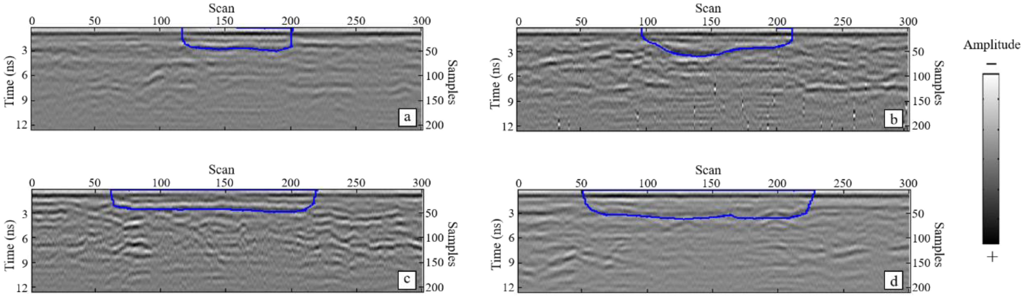
Furthermore, the predicted results of the testing dataset were compared with the ground truth, and the IoU of the model on the testing dataset was calculated and divided into two classes according to Section 2.4:
- When , a good prediction is obtained. The target region was successfully segmented, and the borders fit well (the yellow arrows in Figure 8a–d). In a few cases, as indicated by the red arrow on the right in Figure 8b, the output of U-Net was better than the manual ground truth. The borders of the segmentation masks were slightly different from the manual ground truth (the red arrows in Figure 8c,d) at times, but the error was acceptable, with less than one wavelength.
- When , the segmentation results are weak. Some of the segmentation maps were incomplete, and the boundaries were incorrect, as the red arrows indicate in Figure 8e,f.
The average IoU of the testing dataset was 0.83, indicating that the model could segment the target. The segmentation results of the data collected on 20 May were arranged according to the sequence of profile numbers from small to large, as shown in Figure 9, corresponding to west to east. In addition, the direction of each mask is from south to north.
3.2. Monitoring
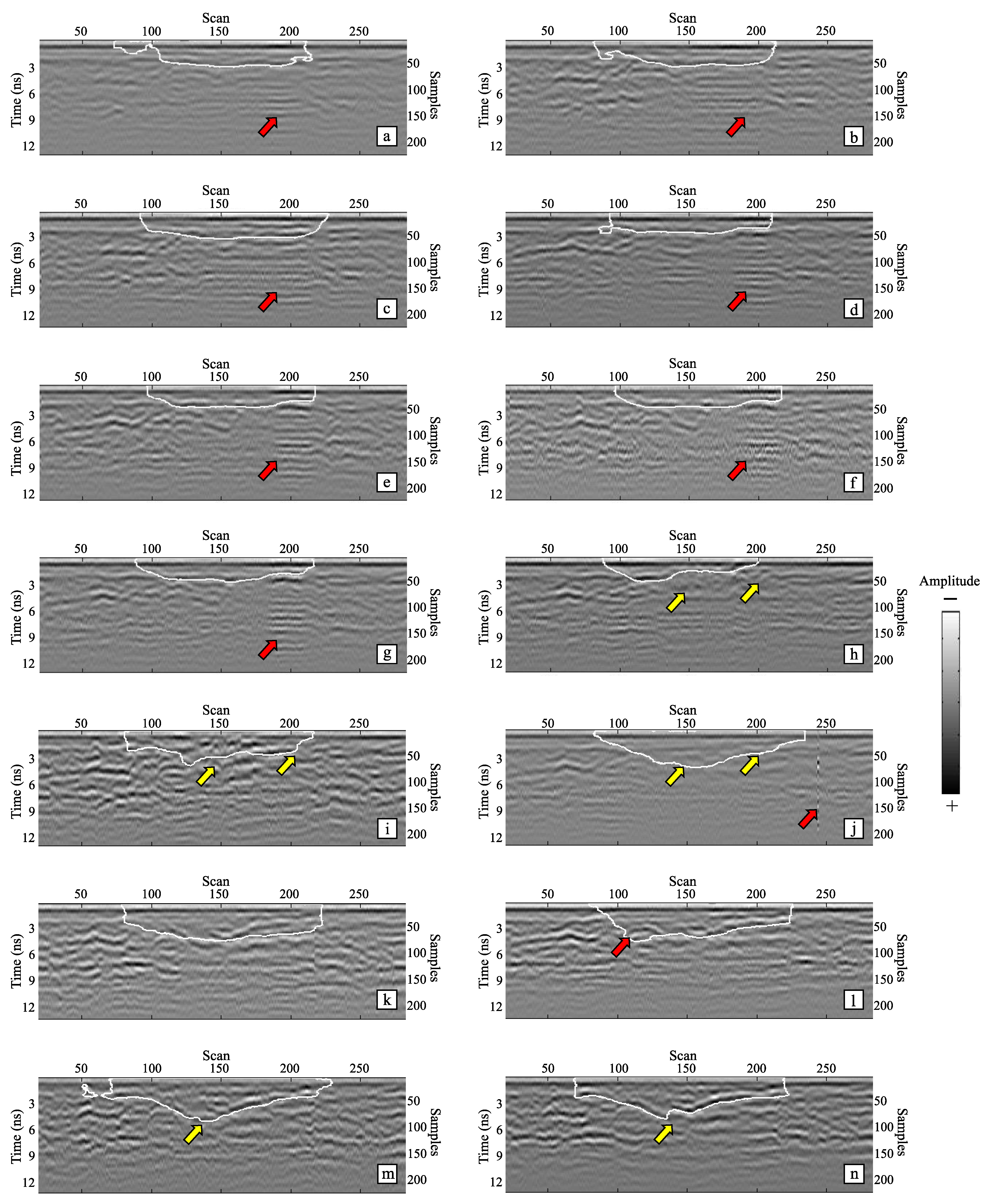
P50 profiles were used as an example to show the changes in the data. As shown in Figure 10a–g, the borders were approximately “U”-shaped. However, a gradual change to a “V” shape of the borders (yellow arrows) was observed, as shown in Figure 10h–j.
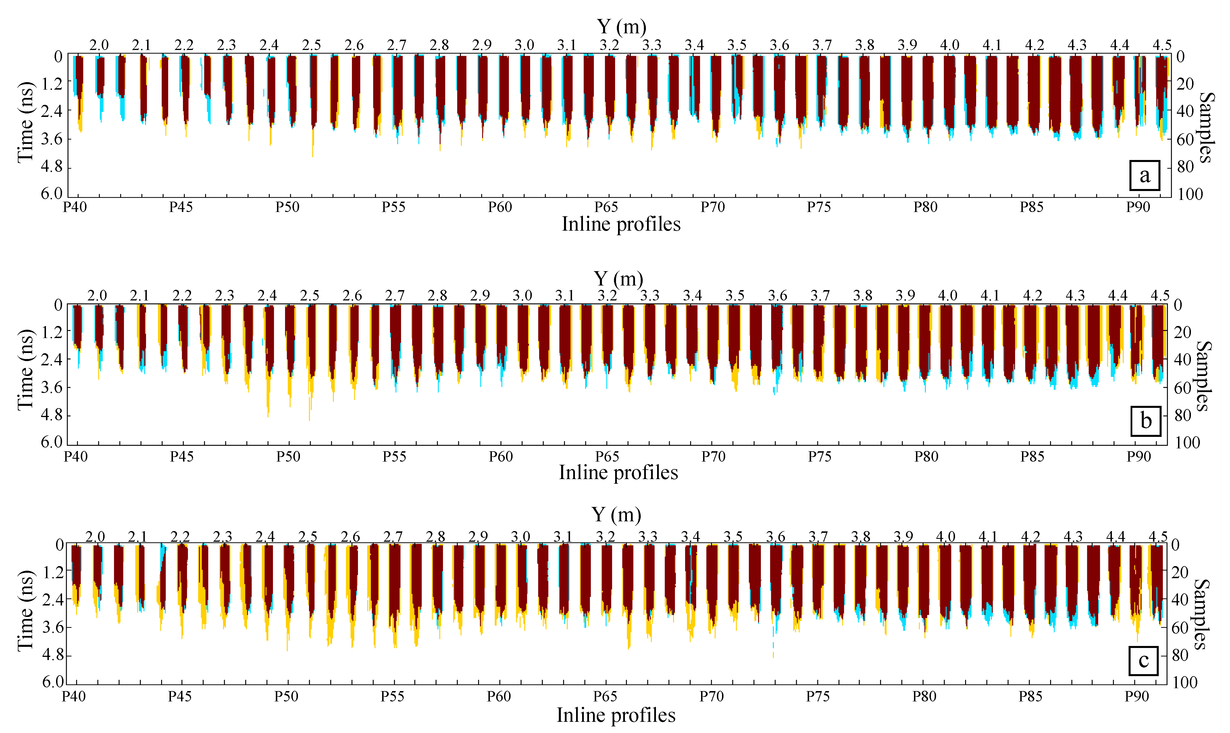
To further determine the changes in the 3D data, the overlapped masks on 4 June, 22 August, and 26 September are listed in a crossline direction, as shown in Figure 11, in which changes are shown in blue and yellow, and unchanged areas in red.
- June 4: As shown in Figure 11a, changes in the left and right borders are noted on the blue masks from Y = 1.95 m to Y = 2.25 m, and changes in the bottom borders can be seen on the yellow masks from Y = 2.35 m to Y = 3.35 m.
- August 8: As shown in Figure 11b, a significant change in the lateral boundaries can be seen from Y = 2.10 m to Y = 2.65 m and from Y = 3.00 m to Y = 4.50 m (yellow masks in Figure 11b). The bottom borders also change from Y = 2.10 m to Y = 2.65 m (yellow masks) and from Y = 3.90 m to Y = 4.40 m (blue masks).
4. Discussion
4.1. Did the Backfill Pit Really Change?
The time-lapse changes in this study refer to the segmentation masks in the preprocessed radar data, as mentioned in Section 2.5. They provide a sense of lateral variation in the shallow targets, but the changes cannot be accurately calculated because the two-way travel time is not linked to depth, which is crucial information for interpreting GPR data, as the propagation velocity is unknown. For a two-layer model with a horizontal interface, the propagation velocity of the first layer can be calculated using the common middle point (CMP). However, the bottom of this backfill pit was neither irregular nor clear; thus, the speed cannot be calculated using this nondestructive detection method. Moreover, experimental conditions prevented the sampling and laboratory analysis of the material in the backfill pit. Given that the goal of this study was to discuss the fast segmentation of GPR data using U-Net and provide an idea of data comparisons, the study of velocity is not the focus of this study.
For all time-lapse detections, we attempted to avoid rainfall and select similar dry weather for data collection to avoid the influence of water content on speed as much as possible. However, for the rainy season, such as August, the water content and dielectric constant of the subgrade could be higher than during other times; thus, the main frequency and speed of the radar signal may be reduced. On the radar profile, the position of the upper border may be seen further downward, creating a “deepening” illusion, such as the significant expansion of bottom borders from Y = 1.95 m to Y = 3.70 m in Figure 11c. However, if the propagation velocity has not changed dramatically, this phenomenon must be caused by the deepening of the backfill pit. In this case, the backfill pit may have been refilled in August, because it expanded significantly more in September than in May, unlike in August or earlier. Settlement may have occurred in the backfill pit after being rolled, leading to the deformation of the road, and the subgrade may have been filled to facilitate the passage of engineering vehicles. Nonetheless, lateral changes are still valuable since the positions of survey lines were kept unchanged among the time-lapse detections.
4.2. Outlook
Previous studies have used neural networks to recognize targets [5] instead of segmented images [15,16]. The goal of GPR is to identify the range of a target; thus, the network should be capable of both recognition and segmentation. However, most studies remain focused on recognizing strong reflected signals, such as diffraction waves and antenna ringing [9,11]. This is because the result of semi-supervised segmentation is highly dependent on ground truths, which are manually annotated. The complex signals and variable features of GPR data introduce difficulties in annotation and segmentation; thus, methods are expected to be applied to identify the features. For instance, the texture feature coding method was used to extract texture-based features from GPR B-scans [9], and the detection results from the neural network may be more satisfactory with these strong features.
In further research, a dynamic 3D underground database should be realized using TLFC 3D GPR. In this study, TLFC 3D GPR was successfully used to monitor a small field, but the samples and data used to train U-Net were only from the backfill pit in this study. That is, the neural network trained in this study may be inapplicable to targets with other characteristics. If the time-lapse detection can be conducted in a large area to collect more target samples, a more universal neural network model can be established to achieve the segmentation and monitoring of multiple targets.
5. Conclusions
In this study, U-Net was used to segment the inline GPR profiles and divide the boundary of the target backfill pit. After 432 training sessions, an effective and available network model was obtained with IoUs of 0.96 and 0.83 on the training and testing datasets, respectively. This network was used to segment all radar data collected from 20 May to 26 September, and the comparison of segmentation masks with the same location but different acquisition dates provides a method to determine the change in the target.
Author Contributions
Conceptualization, K.S., R.Q. and J.L.; methodology, K.S., J.L., A.S. and J.X.; validation, K.S., R.Q., F.Z., A.S., J.X. and Z.Z.; formal analysis, R.Q., F.Z. and Z.Z.; investigation, K.S. and A.S.; data processing, K.S., J.L., A.S. and J.X.; writing—original draft preparation, K.S. and J.L.; writing—review and editing, K.S., J.L., A.S., F.Z., J.X., Z.Z. and R.Q.; supervision, F.Z. and Z.Z.; project administration, J.L. and J.X.; funding acquisition, R.Q. All authors have read and agreed to the published version of the manuscript.
Funding
This research was funded by Natural Science Foundation of Beijing Municipality (8212016).
Data Availability Statement
Data associated with this research are available and can be obtained by contacting the corresponding author.
Acknowledgments
Zhenning Ma, Jun Zhang, Wenyuan Jin, Xu Liu, Yuchen Wang from China University of Geosciences Beijing are appreciated for their assistance in field experiment.
Conflicts of Interest
The authors declare no conflict of interest.
Appendix A

Table A1.
Dataset and acquisition date (year: 2019; date: MM. DD).
| Datasets | Date | Datasets | Date | Datasets | Date |
|---|---|---|---|---|---|
| (a) | 05.20 | (f) | 08.02 | (k) | 08.30 |
| (b) | 06.04 | (g) | 08.05 | (l) | 09.05 |
| (c) | 06.18 | (h) | 08.08 | (m) | 09.12 |
| (d) | 07.22 | (i) | 08.14 | (n) | 09.26 |
| (e) | 07.30 | (j) | 08.22 | (o) | 10.25 |
Appendix A.1. Raw Data and Misalignments
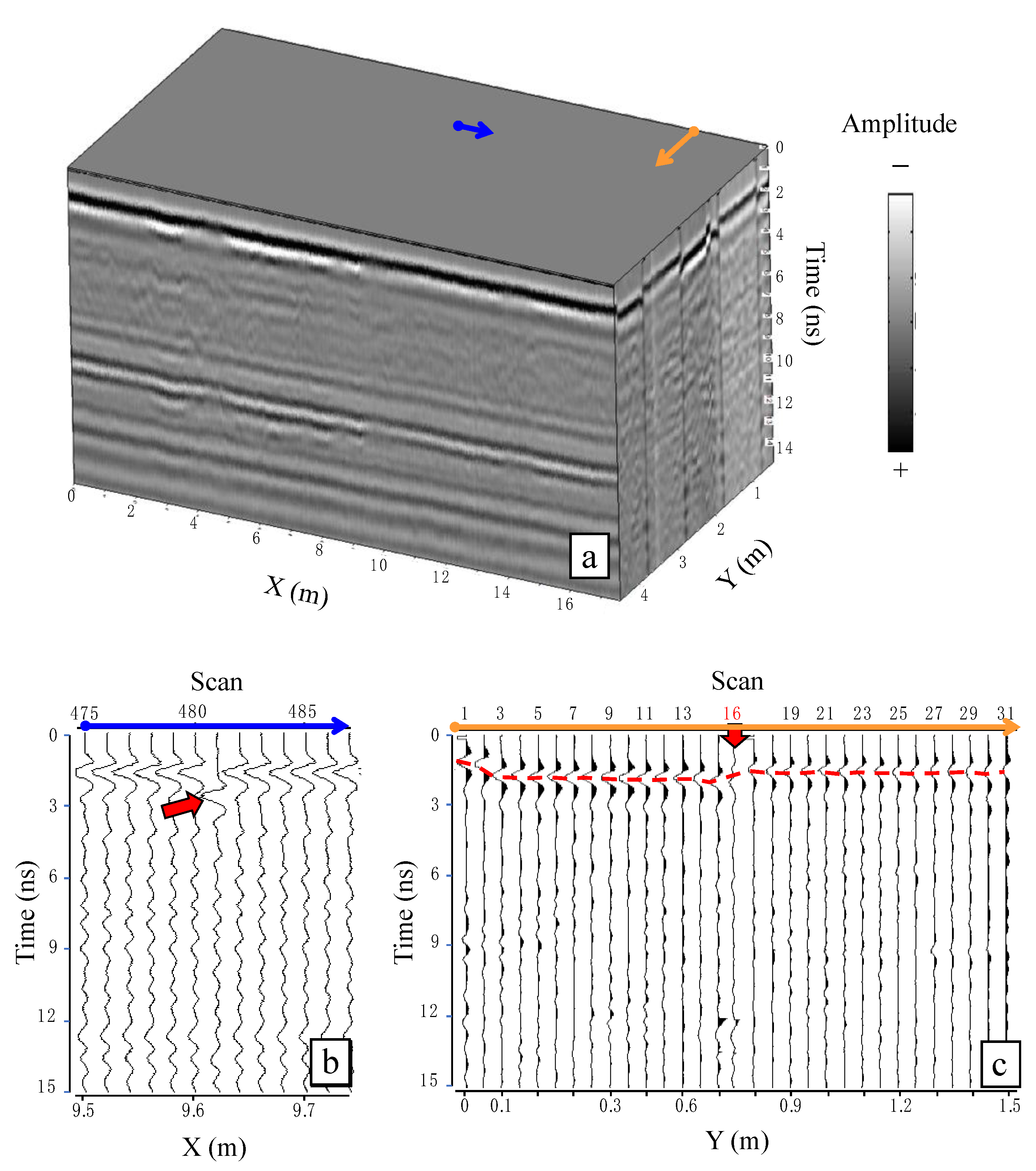
Figure A1.
Three-dimensional display and time zero misalignments of GPR data. (a) The data cube is displayed as an intensity cube. The colored arrows in (b,c) indicate the position and orientation of the profiles in the data cube, corresponding to that in (a). (b) The red arrow indicates the time zero misalignments of the inline, where scans were collected by one antenna. (c) The red dash line indicates the time zero misalignments of the crossline, where scans were collected by an antenna array.

Appendix A.2. Antenna Lifting Test
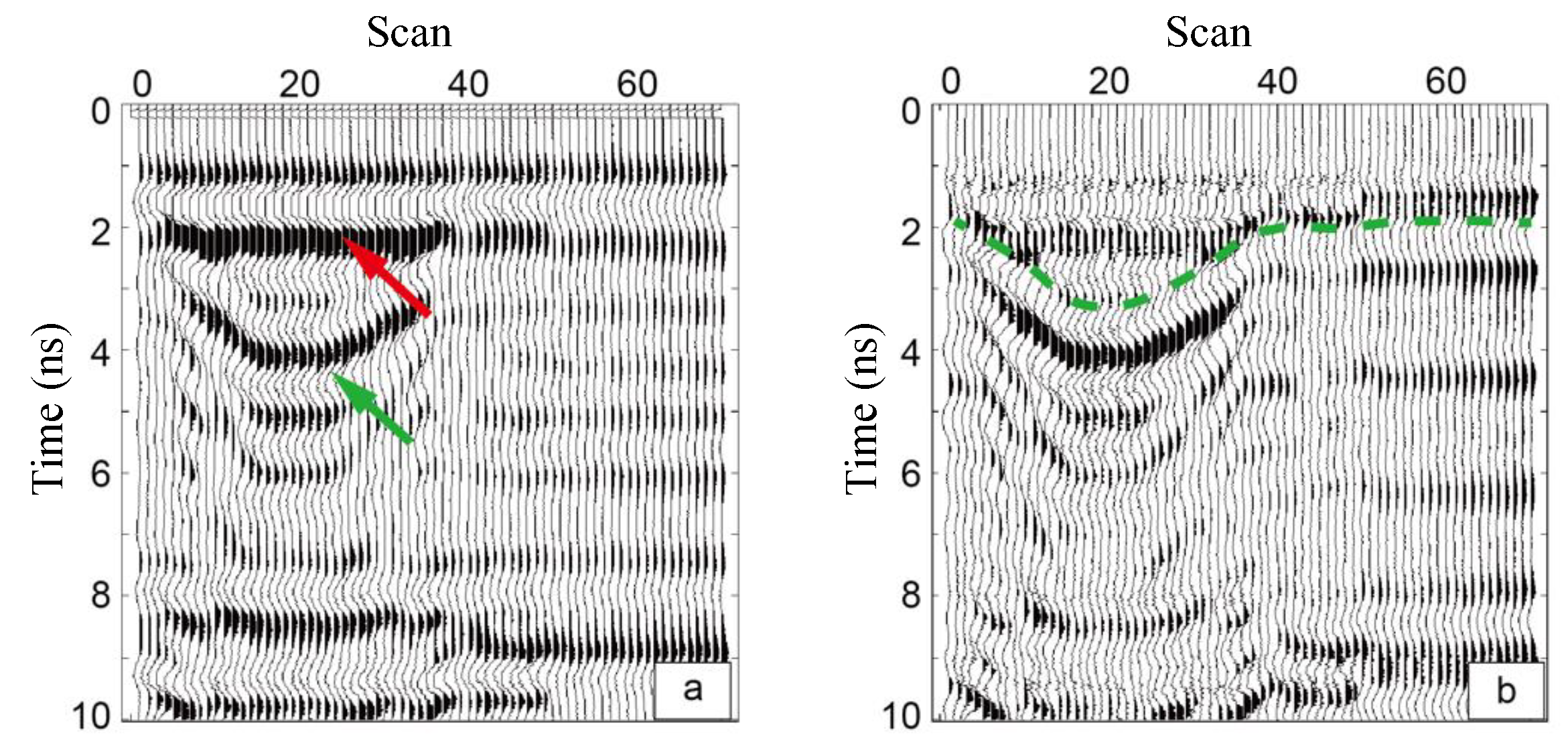
This test was performed in the field prior to each survey by raising the antenna slowly from the ground surface and then returning it to the ground while observing the reflected waveforms as a V-shaped return on a B-scan (Figure A2a). A horizontal BGR filter was applied (Figure A2b) to distinguish positive and negative polarity reflections. Using this method, the direct wave on the ground was separated from the direct wave in the air by picking the first positive peak in the air. Note that there was a slight shift to an earlier time position in the direct wave when the antenna was on the ground surface, as the green dashed line shows on the right side of Figure A2b. The antenna lifting test was conducted several times, and the average reflection time was set as the time zero.
Figure A2.
Antenna lifting test. (a) Direct wave in air (red arrow) and reflected wave on the ground (green arrow) in the raw data. (b) BGR filter and time zero (green dashed line).
Figure A2.
Antenna lifting test. (a) Direct wave in air (red arrow) and reflected wave on the ground (green arrow) in the raw data. (b) BGR filter and time zero (green dashed line).

Appendix A.3. Preprocessing on Inline Profiles
Figure A3.
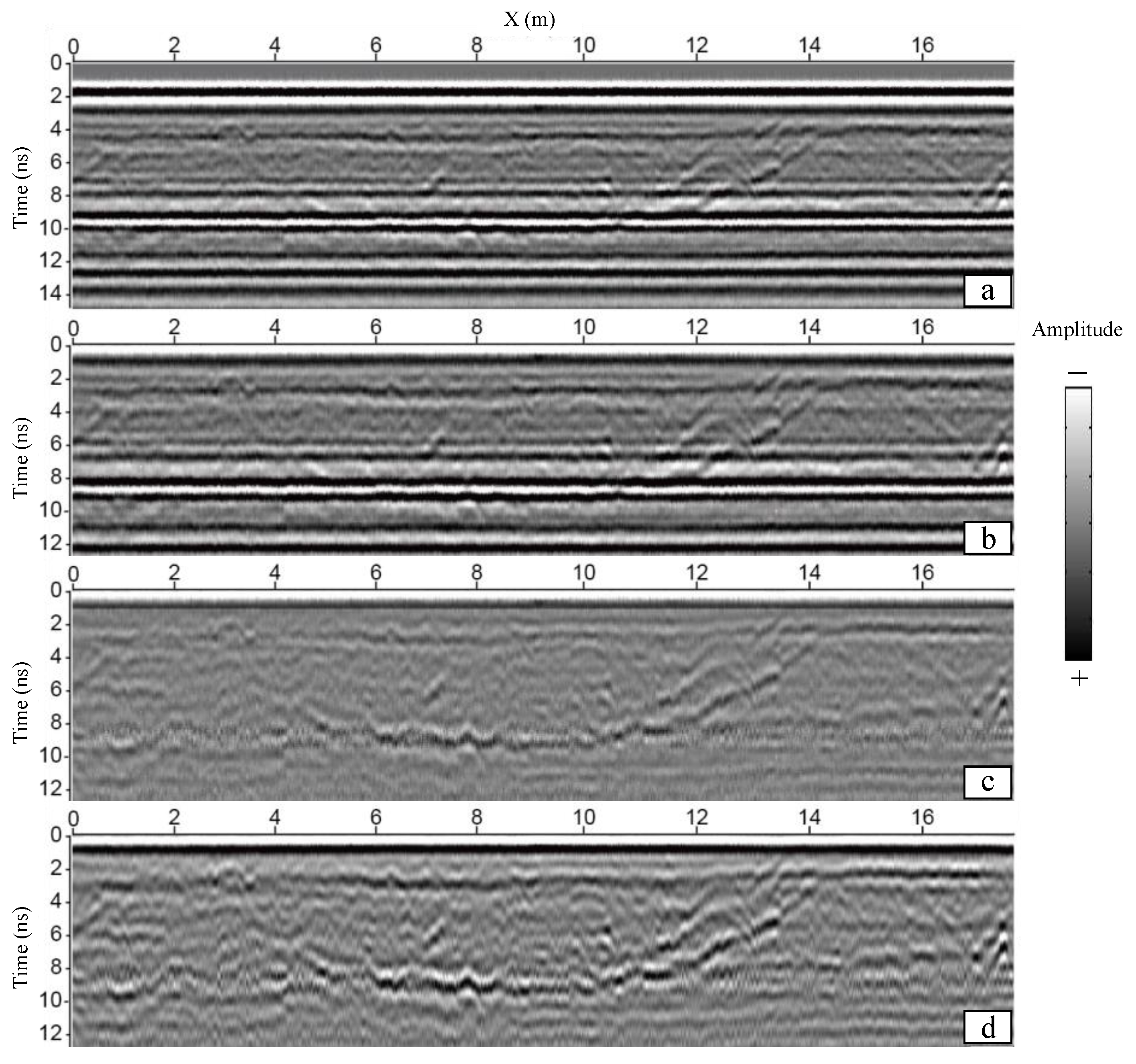
Raw data and preprocessed data of inline profile. (a) Raw data. (b) After time zero correction. (c) After BGR filter. (d) After frequency filter.
Figure A3.
Raw data and preprocessed data of inline profile. (a) Raw data. (b) After time zero correction. (c) After BGR filter. (d) After frequency filter.

Appendix A.4. Three-Dimensional Time Zero Normalization
The cross-correlation sequence of the direct wave between and was calculated according to Equation (A1), where the value is obtained when is maximum.
where is a reference GPR signal with a known direct wave travel time, and is the signal to be matched.
Figure A4.
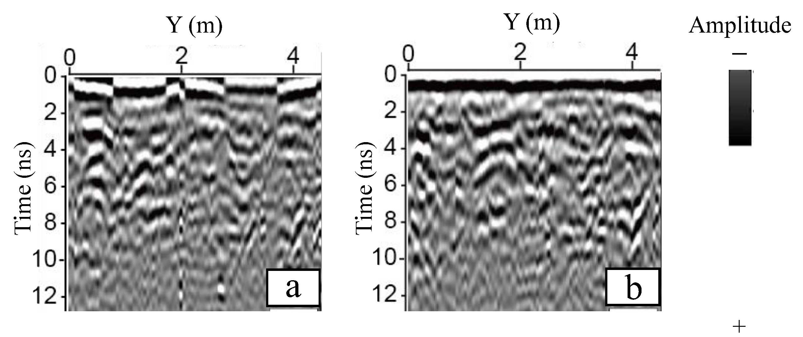
Raw data and preprocessed data of crossline profile. (a) Raw data. (b) After 3D time zero correction.
Figure A4.
Raw data and preprocessed data of crossline profile. (a) Raw data. (b) After 3D time zero correction.

Appendix A.5. Three-Dimensional Data Combination and Imaging
The correlation coefficient of all the overlapping scans was calculated according to Equation (A2).
where and are the scan numbers, is the number of sampling points of each scan, and and denote the reference signals and the signals to be spliced, respectively. When the maximum value of is obtained, it is considered that the scan in corresponds to the same position of the trace in , and the scan numbers of and are recorded as and , respectively. The scan numbers corresponding to the same position were subtracted and averaged according to Equation (A3) to obtain the relative offset .
The offset between adjacent group lines was successively calculated and moved along the Y direction to obtain the data cube after combination.
Figure A5.
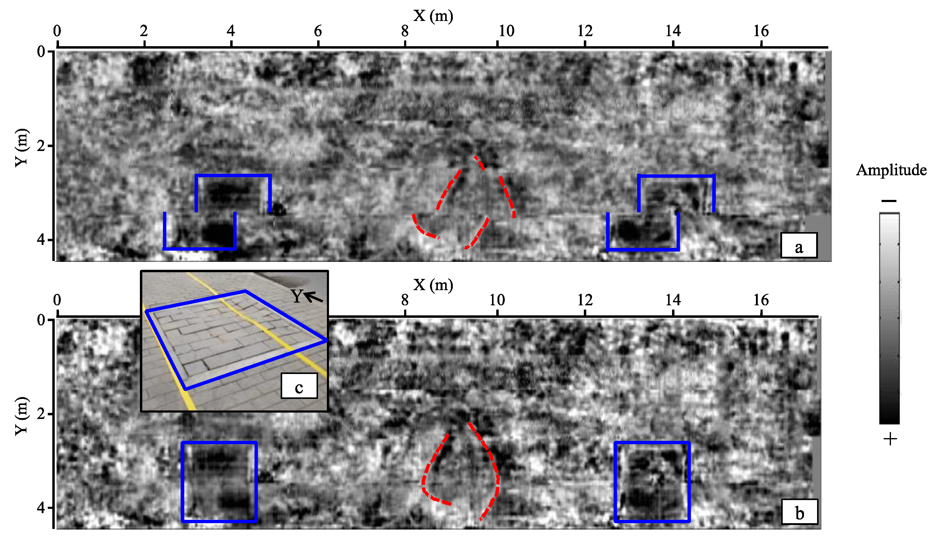
Time slice of 3D GPR data at . The blue boxes indicate the boundaries of two square backfill pits, and the red dash lines indicate the borders of the backfill pit which was segmented in this study. (a) Time slice before data combination. There is a significant misplacement at and , as data were collected from different group lines. (b) Time slice after data combination. The misplacement was rectified by the correlation applied to the overlapping data of adjacent group lines. The backfill pits marked by the blue boxes are clearly visible and easy to be located on the radar slice and can be used to match the position of the time-lapse data. (c) The square backfill pit.
Figure A5.
Time slice of 3D GPR data at . The blue boxes indicate the boundaries of two square backfill pits, and the red dash lines indicate the borders of the backfill pit which was segmented in this study. (a) Time slice before data combination. There is a significant misplacement at and , as data were collected from different group lines. (b) Time slice after data combination. The misplacement was rectified by the correlation applied to the overlapping data of adjacent group lines. The backfill pits marked by the blue boxes are clearly visible and easy to be located on the radar slice and can be used to match the position of the time-lapse data. (c) The square backfill pit.

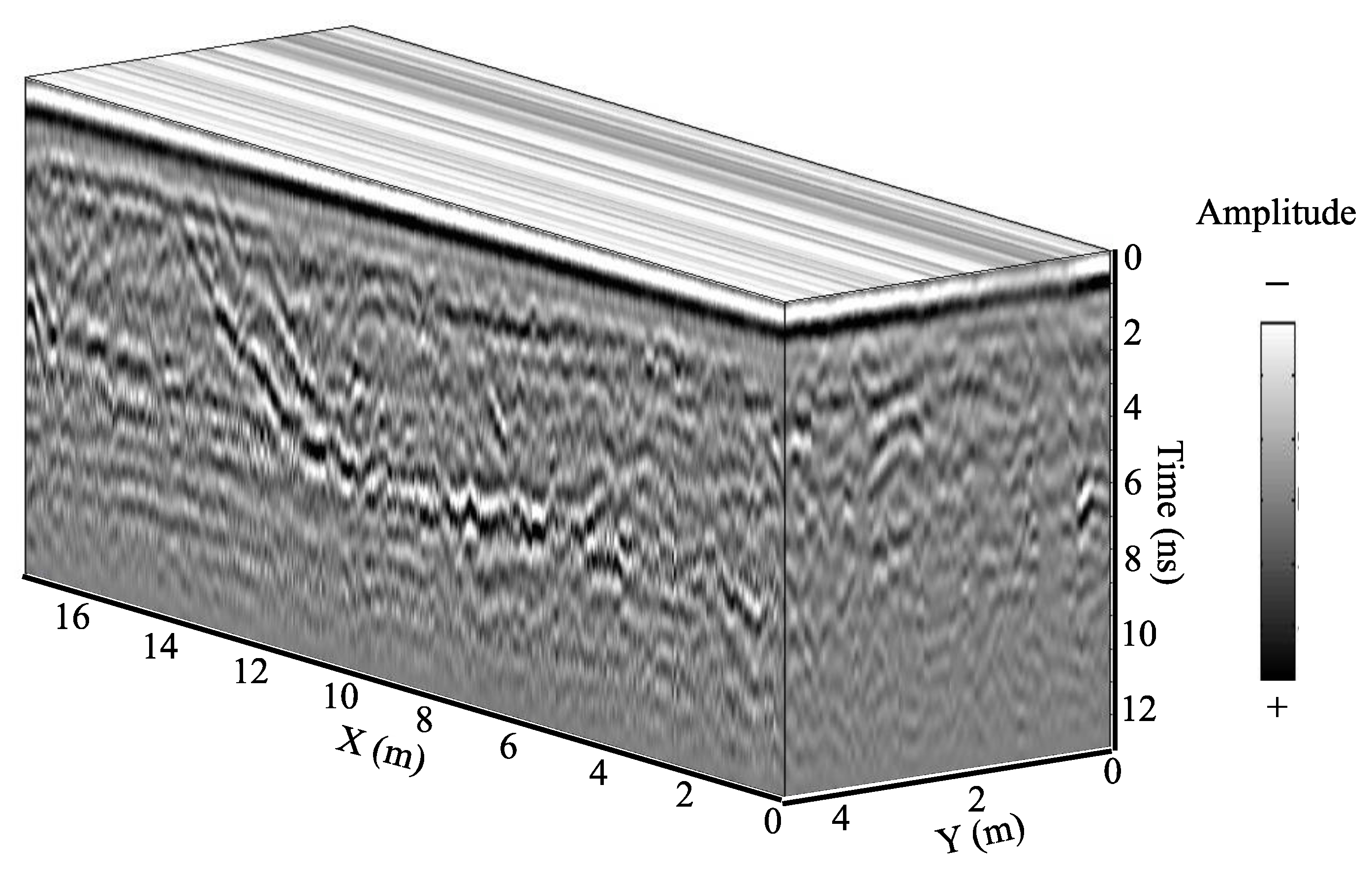
Figure A6.
Three-dimensional GPR data cube after preprocessing.

References
- Reeves, B.A.; Muller, W.B. Traffic-speed 3-D noise modulated ground penetrating radar (NM-GPR). In Proceedings of the 2012 14th International Conference on Ground Penetrating Radar, Shanghai, China, 4–8 June 2012; pp. 165–171. [Google Scholar] [CrossRef]
- Simonin, J.M.; Baltazart, V.; Hornych, P.; Dérobert, X.; Thibaut, E.; Sala, J.; Utsi, V. Case study of detection of artificial defects in an experimental pavement structure using 3D GPR systems. In Proceedings of the 15th International Conference on Ground Penetrating Radar, Brussels, Belgium, 30 June–4 July 2014; pp. 847–851. [Google Scholar] [CrossRef]
- Linjie, W.; Jianyi, Y.; Ning, D.; Changjun, W.; Gao, G.; Haiyang, X. Analysis of interference signal of ground penetrating radar in road detection. J. Hubei Polytech. Univ. 2017, 33, 35–40. [Google Scholar] [CrossRef]
- Simonyan, K.; Zisserman, A. Very deep convolutional networks for large-scale image recognition. arXiv 2014, arXiv:1409.1556. [Google Scholar]
- Russakovsky, O.; Deng, J.; Su, H.; Krause, J.; Satheesh, S.; Ma, S.; Huang, Z.; Karpathy, A.; Khosla, A.; Bernstein, M.; et al. ImageNet large scale visual recognition challenge. Int. J. Comput. Vis. 2014, 45, 211–252. [Google Scholar] [CrossRef]
- Tompson, J.; Jain, A.; Lecun, Y.; Bregler, C. Joint training of a convolutional network and a graphical model for human pose estimation. arXiv 2014, arXiv:1406.2984. [Google Scholar]
- Girshick, R.; Donahue, J.; Darrell, T.; Malik, J. Region-based convolutional networks for accurate object detection and segmentation. IEEE Trans. Pattern Anal. Mach. Intell. 2016, 38, 142–158. [Google Scholar] [CrossRef] [PubMed]
- Shan, K.; Guo, J.; You, W.; Lu, D.; Bie, R. Automatic facial expression recognition based on a deep convolutional-neural-network structure. In Proceedings of the IEEE International Conference on Software Engineering Research, London, UK, 7–9 June 2017; pp. 123–128. [Google Scholar] [CrossRef]
- Besaw, L.E.; Stimac, P.J. Deep convolutional neural networks for classifying GPR B-Scans. In Proceedings of the SPIE the International Society for Optical Engineering, San Diego, CA, USA, 9–13 August 2015; SPIE: Bellingham, WA, USA, 2015; Volume 9454. [Google Scholar] [CrossRef]
- Lameri, S.; Lombardi, F.; Bestagini, P.; Lualdi, M.; Tubaro, S. Landmine detection from GPR data using convolutional neural networks. In Proceedings of the 2017 25th European Signal Processing Conference (EUSIPCO), Kos, Greece, 26 October 2017; pp. 508–512. [Google Scholar] [CrossRef]
- Kim, N.; Kim, S.; An, Y.K.; Lee, H.J.; Lee, J.J. Deep learning-based underground object detection for urban road pavement. Int. J. Pavement Eng. 2020, 21, 1638–1650. [Google Scholar] [CrossRef]
- Kim, N.; Kim, S.; An, Y.K.; Lee, J.J. A novel 3D GPR image arrangement for deep learning-based underground object classification. Int. J. Pavement Eng. 2021, 22, 740–751. [Google Scholar] [CrossRef]
- Klesk, P.; Godziuk, A.; Kapruziak, M.; Olech, B. Fast analysis of C-scans from ground penetrating radar via 3-D haar-like features with application to landmine detection. IEEE Trans. Geosci. Remote Sens. 2015, 53, 3996–4009. [Google Scholar] [CrossRef]
- Jing, H.; Vladimirova, T. Novel algorithm for landmine detection using C-scan ground penetrating radar signals. In Proceedings of the 2017 Seventh International Conference on Emerging Security Technologies (EST), Canterbury, UK, 6–8 September 2017; pp. 68–73. [Google Scholar] [CrossRef]
- Ronneberger, O.; Fischer, P.; Brox, T. U-net: Convolutional networks for biomedical image segmentation. In Medical Image Computing and Computer-Assisted Intervention–MICCAI 2015, Proceedings of the 8th International Conference, Munich, Germany, 5–9 October 2015; Lecture Notes in Computer Science; Springer: Cham, Switzerland, 2015; Volume 9351, p. 9351. [Google Scholar] [CrossRef]
- Berezsky, O.; Pitsun, O.; Derysh, B.; Pazdriy, I.; Melnyk, G.; Batko, Y. Automatic segmentation of immunohistochemical images based on U-net architecture. In Proceedings of the 2021 IEEE 16th International Conference on Computer Sciences and Information Technologies (CSIT), Lviv, Ukraine, 22–25 September 2021; pp. 29–32. [Google Scholar] [CrossRef]
- Ling, J.; Qian, R.; Shang, K.; Guo, L.; Zhao, Y.; Liu, D. Research on the dynamic monitoring technology of road subgrades with time-lapse full-coverage 3D ground penetrating radar (GPR). Remote Sens. 2022, 14, 1593. [Google Scholar] [CrossRef]
Figure 1.
Detection coverage and 3D GPR slice. Data were collected on 8 August 2019. The double travel time of the slice is 1.464 ns.
Figure 1.
Detection coverage and 3D GPR slice. Data were collected on 8 August 2019. The double travel time of the slice is 1.464 ns.

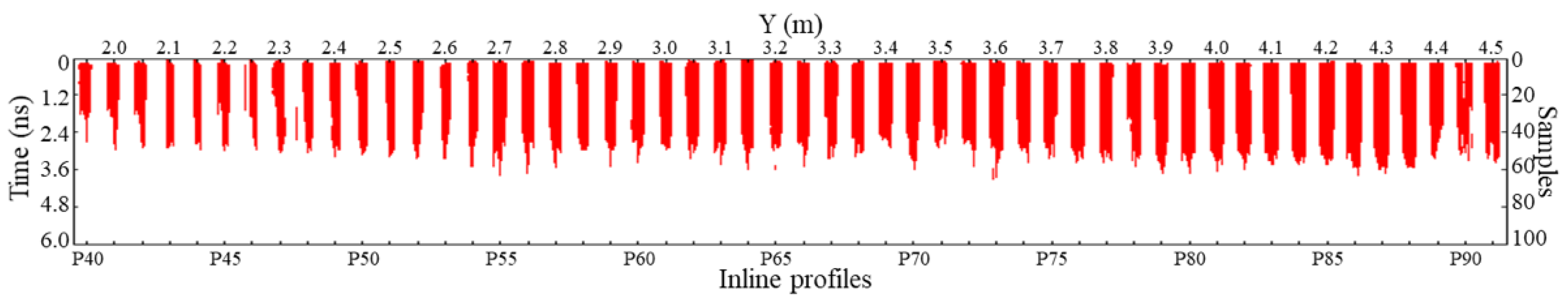
Figure 2.
Survey lines of the TLFC 3D GPR acquisition and the raw data of inline profiles. Data were collected on 8 August 2019.
Figure 2.
Survey lines of the TLFC 3D GPR acquisition and the raw data of inline profiles. Data were collected on 8 August 2019.

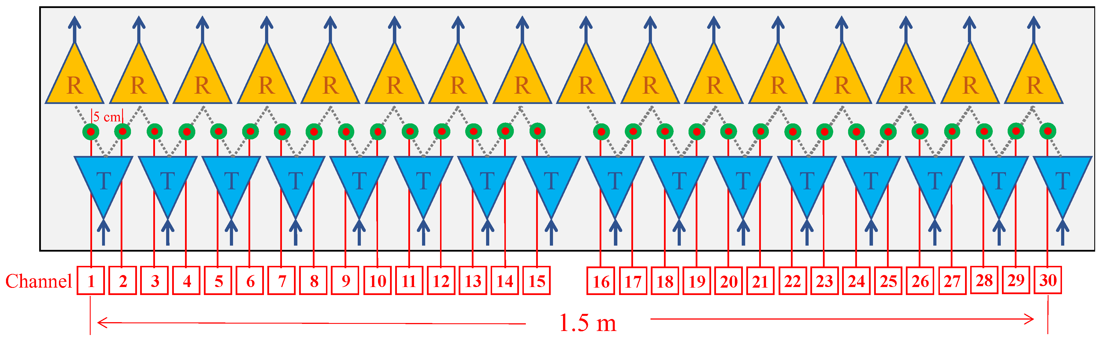
Figure 3.
Antenna array of the MobyScan-V. There are 16 transmitters (blue triangles) and 16 receivers (yellow triangles). Red dots with green borders indicate the GPR channels between transmitters and receivers. The distance between channels 15 and 16 is 10 cm, and the data here were interpolated to achieve uniform spatial sampling.

Figure 4.
The classic U-Net architecture. The model comprises contracting and expansive pathways, with skip connections between the corresponding layers.
Figure 4.
The classic U-Net architecture. The model comprises contracting and expansive pathways, with skip connections between the corresponding layers.

Figure 5.
IoU is the ratio of overlap to union of the ground truth (green box) and the segmentation result (red box).
Figure 5.
IoU is the ratio of overlap to union of the ground truth (green box) and the segmentation result (red box).

Figure 6.
Changes in the target are shown by overlapping the masks. (a) Segmentation mask P1; (b) segmentation mask P2; (c) results of comparison by overlapping P1 and P2. The blue mask marked with “S” indicates the part in P1 which is not seen at the same position in P2; the yellow mask marked with “E” indicates the part that does not appear in P1 but is seen in P2.

Figure 7.
Data annotation of the target backfill pit: (a) profile P44; (b) profile P54; (c) profile P69; (d) profile P87.
Figure 7.
Data annotation of the target backfill pit: (a) profile P44; (b) profile P54; (c) profile P69; (d) profile P87.

Figure 8.
Typical examples of the accuracy of the testing dataset prediction results; the white curves are the boundaries of the segmentation masks, and the blue curves are the boundaries of the manual ground truth. (a) Profile P87, IoU = 0.89; (b) profile P62, IoU = 0.89; (c) profile P61, IoU = 0.87; (d) profile P50, IoU = 0.80; (e) profile P69, IoU = 0.57; (f) profile P55, IoU = 0.64.

Figure 9.
Segmentation results of data collected on 20 May. The horizontal axis represents the y-coordinate and the number of inline profiles, and the segmentation masks of the backfill pit are in red.
Figure 9.
Segmentation results of data collected on 20 May. The horizontal axis represents the y-coordinate and the number of inline profiles, and the segmentation masks of the backfill pit are in red.

Figure 10.
Segmentation results of time-lapse data of the P50 profiles. (a–n) are the P50 profiles from 20 May to 26 September. The date and subplot number correspond to those in Table A1. The segmentation was not affected by interferences from multiple reflections (red arrow in (a–g)) or a dead signal (red arrow in (j)). In a few cases, the segmentation slightly deviated from an ideal performance (red arrow in (l)).

Figure 11.
Comparison between segmentation masks: (a) 4 June, at Y = 4.45 m, yellow and blue masks within the red mask indicate the incompleteness of the reference mask rather than the change in the target; (b) 22 August; (c) 26 September, the blue masks in the upper left at Y = 2.15 m and in the middle at Y = 3.40 m are caused by mis-segmentation in the 26 September data, rather than changes.

Table 1.
The technical specifications of the MobyScan-V and data acquisition parameters.
| Indicators | Parameters |
|---|---|
| Antenna type | Ground-coupled antenna arrays |
| Number of channels | 30 |
| Center Frequency | 2 GHz |
| Channels spacing (crossline) | 0.05 m |
| Scans spacing (inline) | 0.02 m |
| Sampling points | 512 |
| Time window | 15 ns |
Table 2.
Preprocessing steps and parameters.
| Step | Processing Method | Parameter/Object |
|---|---|---|
| Time zero correction | Antenna lifting test | 2 ns |
| Background removal (BGR) | Sliding window | 150 scans |
| Frequency filtering | Butterworth filter | 500–1500 MHz |
| 3D time zero normalization | Correlation | Direct-coupling |
| 3D data combination | Correlation | Overlapping data |
Table 3.
Information of the training and testing datasets.
| Training Dataset | Testing Dataset | |
|---|---|---|
| Number | 249 | 52 |
| Sampling points of GPR data | 16,434,000 | 3,432,000 |
| Proportion of total data | 19.5% | 7.1% |
| Data acquisition date | 20 May 2019–26 September 2019 | 25 October 2019 |
Publisher’s Note: MDPI stays neutral with regard to jurisdictional claims in published maps and institutional affiliations. |
© 2022 by the authors. Licensee MDPI, Basel, Switzerland. This article is an open access article distributed under the terms and conditions of the Creative Commons Attribution (CC BY) license (https://creativecommons.org/licenses/by/4.0/).
Share and Cite
MDPI and ACS Style
Shang, K.; Zhang, F.; Song, A.; Ling, J.; Xiao, J.; Zhang, Z.; Qian, R. Fast Segmentation and Dynamic Monitoring of Time-Lapse 3D GPR Data Based on U-Net. Remote Sens. 2022, 14, 4190. https://doi.org/10.3390/rs14174190
AMA Style
Shang K, Zhang F, Song A, Ling J, Xiao J, Zhang Z, Qian R. Fast Segmentation and Dynamic Monitoring of Time-Lapse 3D GPR Data Based on U-Net. Remote Sensing. 2022; 14(17):4190. https://doi.org/10.3390/rs14174190
Chicago/Turabian StyleShang, Ke, Feizhou Zhang, Ao Song, Jianyu Ling, Jiwen Xiao, Zihan Zhang, and Rongyi Qian. 2022. "Fast Segmentation and Dynamic Monitoring of Time-Lapse 3D GPR Data Based on U-Net" Remote Sensing 14, no. 17: 4190. https://doi.org/10.3390/rs14174190
Note that from the first issue of 2016, this journal uses article numbers instead of page numbers. See further details here.