
Mesoscale Eddies in the Black Sea and Their Impact on River Plumes: Numerical Modeling and Satellite Observations


1
Shirshov Institute of Oceanology, Russian Academy of Sciences, Nakhimovskiy Prospect 36, 117997 Moscow, Russia
2
Moscow Institute of Physics and Technology, Institusky Lane 9, 141701 Dolgoprudny, Russia
*
Author to whom correspondence should be addressed.
Remote Sens. 2022, 14(17), 4149; https://doi.org/10.3390/rs14174149
Submission received: 2 July 2022
/
Revised: 6 August 2022
/
Accepted: 16 August 2022
/
Published: 24 August 2022
(This article belongs to the Special Issue Recent Advancements in Remote Sensing for Ocean Current)
Abstract
:The Northeast Caucasian Current (NCC) is the northeastern part of the cyclonic Rim Current (RC) in the Black Sea. As it sometimes approaches the narrow shelf very closely, topographically generated cyclonic eddies (TGEs) can be triggered. These eddies contribute to intense, along- and cross-shelf transport of trapped water with enhanced self-cleaning effects of the coastal zone. Despite intense studies of eddy dynamics in the Black Sea, the mechanisms of the generation of such coastal eddies, their unpredictability, and their capacity to capture and transport impurities are still poorly understood. We applied a 3-D low-dissipation model DieCAST/Die2BS coupled with a Lagrangian particle transport model supported by analysis of optical satellite images to study generation and evolution of TGEs and their effect on river plumes unevenly distributed along the northeastern Caucasian coast. Using the Furrier and wavelet analyses of kinetic energy time series, it was revealed that the occurrence of mesoscale TGEs ranges from 10 up to 50 days. We focused on one particular isolated anticyclonic TGE that emerged in late fall as a result of instability of the RC impinging on the abrupt submarine area adjoining the Pitsunda and Iskuria capes. Being shed, the eddy with a 30-km radius traveled along the coast as a coherent structure during ~1.5 months at a velocity of ~3 km/day and vertical vorticity normalized by the Coriolis parameter ~(0.1 ÷ 1.2). This eddy captured water from river plumes localized along the coast and then ejected it to the open sea, providing an intense cross-shelf transport of riverine matter.
1. Introduction
Coastal mesoscale eddies widely emerging in the ocean play an important role in physical, biological, and geochemical processes. They may considerably affect transport, accumulation, and dispersion of pollutants [1,2,3], floating organisms [4,5,6,7,8], phytoplankton [9], and microplastic pollution in the sea, which have received large attention during the last decade [10,11,12].
In this study, we focus on mesoscale eddies in the semi-enclosed Black Sea. Being one of the main features of the general Black Sea circulation, the basin-scale cyclonic boundary current, referred to as the Rim Current (RC), is forced by the local wind curl together with thermohaline circulation driven by non-uniform surface fluxes [13,14,15,16,17,18,19,20]. Analysis of extensive CTD and ADCP measurements together with satellite observations revealed that the RC is a well-pronounced meandering jet stream confined over the steepest topographic slope which separates shelf areas and often associated cyclonic–anticyclonic eddy pairs located on both of its sides [17,21,22,23].
The strong-boundary RC limits the water and matter exchange between the shelf and open sea. On the other hand, meandering of the RC and the resulting formation of instabilities manifested by mesoscale eddies, filaments, dipole structures, etc., could significantly enhance the cross-shelf exchange [19,24,25]. Moreover, mesoscale anticyclonic eddies and meanders can capture coastal waters which are rich in nutrients and contaminants and drag them along the coast and/or to the central part of the basin [3,21,22,23,26,27,28].
During the last few decades, the occurrence and behavior of near-shore mesoscale eddies (NAEs) in different regions of the Black Sea received much attention [17,19,21,22,25,26,27,28,29,30,31,32,33]. Despite the encouraging progress in this field, these studies were mostly limited to the registration and calculation of general statistical characteristics of these eddies, including their size, velocity, and existence time [32,33,34,35]. There was neither detailed scrutiny nor analysis of conditions that could play a significant role in eddy generation and, particularly, in generation of topographic eddies, though we should note some works shedding light on the latter. Rachev and Stanev [36] introduced results of numerical simulations indicating that alterations of bottom topography in certain regions lead to notable changes of mesoscale circulation. It results in an increase or decrease of emerged mesoscale eddies, which reveals the strict control of the eddy genesis by sea bottom and coastline morphology. A similar effort to use the altered bottom topography to reveal the influence of the alteration on dynamic instability was applied by Cushman-Roisin et al. [37] in numerical simulations of the Adriatic Sea. This study revealed that near-shore meandering reached larger amplitudes in case of flattened bottom, albeit this factor does not affect the existence and wavelengths of meanders. In other words, offshore displacement is less restrained over a flat bottom than on a sloping shelf because it is not accompanied by vertical stretching and the consequent development of relative vorticity as required by potential vorticity conservation. Finally, recent numerical modeling by Aleskerova et al. [38] together with high-resolution satellite imagery addressed the controlling effect of topography on the mesoscale eddy genesis and revealed typical eddy structure distribution around the Crimean Peninsula.
A very important issue for coastal oceanography is to predict the periodicity of the occurrence of specific types of near-shore eddies, so-called topographically generated eddies (TGE). TGE are often observed in the regions with topographic features at the coastline, such as islands, peninsulas, and capes [39,40,41]. The various causes of current instability and the occurrence of TGE are summarized in [42] and confirmed by laboratory experiments [43,44,45] and numerical experiments [46,47,48].
In the Black Sea, abrupt irregularities of bottom topography and coastline significantly affect the strong coastal jet stream of the RC. The latter, flowing over (and impinging on) such irregularities, causes the formation of instabilities and thus produces coherent eddies and/or eddy chains on the leeward side of the streamlined obstacles. This effect could be enhanced by local river discharges and the resulting thermohaline gradients. Such processes were investigated by laboratory experiments by Elkin and Zatsepin [49] and by numerical experiments by Zhurbas et al. [50].
A role of eddies in transporting materials across the shelf to the open ocean is still poorly understood, particularly when it concerns river discharge and the related interaction between eddies and river plumes. To better understand their role in transporting water mass and materials across the shelf, numerous techniques including Eulerian approaches for various parts of the World Ocean [51] and Lagrangian methods [52] have been developed. For the Black Sea, a combined method based on DieCAST [28,53] and a Lagrangian particle transport model was used to study the effects of the meandering of the RC as well as the generation and motion of anticyclonic eddies on the oil spills [28,54].
In the study, we focus on the northeastern part of the Black Sea, i.e., the Caucasian coastal and shelf zones, where the meandering of the Northeast Caucasian Current (NCC) often approaches the coast very closely [55]. As is shown in the local bathymetry map (Figure 1), at the study area, the shelf northwest from the Pitsunda Cape is very narrow with a steep slope following the shelf [55]. Together with multiple irregularities of the coastline and sea bottom, these conditions are favorable for TGE. Numerous small rivers inflowing the sea along the Caucasian coast form river plumes along the coast, which affect the coastal eddy generation processes and facilitate their visualization at satellite imagery.
First, using spectral analyses, we assess the periodicity of the TGE appearance and study conditions of the eddy trains emerging as a result of the interaction of the RC with bottom topography. Second, in order to understand the mechanisms enabling eddies to efficiently transport coastal waters, we study an individual near-shore isolated anticyclonic eddy, which is representative of anticyclonic eddies in the NCC. Combining a hydrodynamic model with a Lagrangian particle-tracking model, we scrutinize the evolution of this eddy and get new insights into the formation, development, movement, and dissipation of anticyclonic eddies in the study area. Finally, following the approach by Chenillat et al. [56], we study whether this particular eddy is leaky and how long and how far it maintains its coherent signature.
The paper is structured as follows. In Section 2, we describe the region of interest; the DieCAST numerical model; two spectral methods to identify eddy generation and shedding; the Lagrangian particle-tracking method; and satellite data used. In Section 3, the baseline experiments and modeling results are presented; an isolated topographically generated eddy is analyzed in detail. Section 4 (Discussion) is focused on features of the interaction between the eddy and river plumes. Concluding remarks are given in Section 5.
2. Materials and Methods
2.1. Study Area
In this study, we focus on the northeastern part of the Black Sea (Figure 1) where TGEs are often generated. Satellite observations indicate that NAEs most frequently emerge in the area between Sochi and the Iskuria Cape [22,23,29,57], and being shed after emerging, long-lived NAEs propagate along the coast up to Novorossiysk with translation velocity of about 2–4 km/day [55]. The area between Novorossiysk and Iskuria Cape receives freshwater discharge from multiple rivers, which results in interaction of NAEs with buoyant river plumes in the study area [58,59,60,61,62,63,64,65,66,67]. Sometimes NAEs, after protrusion though the RC, move across the shelf towards the Black Sea interior as isolated eddies [3,23,28]. Being captured by eddies, coastal waters along with river-borne pollutants are transported to the open sea, thus facilitating the water exchange between the coastal zone and the open sea.
2.2. Numerical Model
In this work, a 3-D high-resolution (2 nautical miles) low dissipative z-coordinate ocean circulation model DieCAST [53,68] is applied to the Black Sea [54] to study the spectral structure of current velocity with special emphasis on generation, shedding of mesoscale eddies, and their impact on river plumes. We use spectral analysis of current velocity fluctuations to identify frequencies of occurrence of recurrent mesoscale TGEs. Both applied techniques, namely, the Fourier Transform and wavelet techniques, complement each other in identifying coherent mesoscale eddies. To visualize the effects of eddies on river plume behavior, we use a particle-tracking model coupled with the DieCAST [3].
To study the basin scale and mesoscale dynamics of the Black Sea, we use a 2-nautical minute version of the global DieCAST ocean model [53,68]. Similar to the global version, the regional model is also a three-dimensional, z-coordinate, hydrostatic, low dissipative eddy-resolving primitive equation model. This model was adopted for the Black Sea and hereinafter is referred as Die2BS [3]. The model is configured with 30 vertical uneven z-levels, with higher resolution near the surface to resolve upper ocean physics. The bathymetry is derived from an unsmoothed ETOPO2 (http://www.ngdc.noaa.gov/mgg/global/etopo2.html, accessed on 17 July 2022). The physical boundary conditions, initial conditions, and surface forcing used in this study are derived from monthly climatology [3,28,69].
The computational grid of the model covers the entire Black Sea basin from 27.2°E to 42°E and from 40.9°N to 46.6°N and contains a total of 426 238 rectangular cells so that square cell dimensions varied from 2.6 to 2.8 km. Note that for the Black Sea, the first internal baroclinic deformation radius varies from about 5 to 20 km, i.e., significantly less than the square cell; thus, the model enables us to adequately resolve mesoscale and even sub-mesoscale structures.
The Die2BS was initialized with monthly averaged temperature and salinity data and forced with climatological surface buoyancy fluxes, evaporation minus precipitation, monthly winds, and river runoff from the 31 largest rivers [70]. At two open boundaries, namely the Bosporus and Kerch straits, the exchanges are specified as in [3,28,69]. Upon running Die2BS, a special nudging data assimilation procedure was launched. The surface buoyancy flux was computed by nudging both the temperature and the salinity toward monthly climatology as in [19]. For the vertical closeness, a modified version of the Gibson-Launder turbulence model was used [71,72].
In this work, the integration time step was chosen to be equal to 6 min. The model was spun up with the climatological temperature and salinity. The model was run for a total of 39 years with perpetual seasonal forcing to ensure that the basin-averaged kinetic energy, temperature, and basin-scale circulation reach quasi-stationary periodical states. The final state of the physical spin-up was then used as the initial condition of a final 5-year run. Within the last period, daily averages of physical variables were archived and used to explore the main eddy statistics in the Black Sea. To study velocity spectra, we used the daily output of five-year averages of current velocity.
A high-resolution version of Die2BS allows accurately reproducing basin-scale circulation of the Black Sea as central gyres and the quasi-permanent cyclonic RC and its seasonal fluctuations and meandering, as well as upwelling and downwelling events and quasi-stationary large anticyclonic eddies such as Batumi, Sevastopol, Caucasian, etc. High resolution of the model along with extremely low horizontal dissipation (horizontal viscosity ranging from 5 to 10 m2/s) allows the model to realistically reproduce numerous mesoscale and sub-mesoscale eddies and structures such as eddies, filaments, mushroom currents, and jets [3,28,69].
The validation of the circulation model was conducted based on satellite images of sea surface temperature and altimetry data (joint TOPEX/Poseidon and ERS-1/2 data with 0.25° spatial and 10-day temporal resolution) and surface current velocities obtained in observations and derived from drifter experiments. Results of the validation were presented in [3,28,68,69,73]. In addition, we should mention that the previous usage of the same high-resolution resolution version of the DieCAST model for the Adriatic Sea also provided good results for mesostructures when comparing satellite observations and modeling data [37,74].
As shown in previous studies, near-shore eddies generated in the area between the RC and the coast and processes of eddy protrusion into the RC are very important for water and matter exchange between the open sea and the coastal zone [3,22,23]. Note that the low dissipation is very important for reproducing realistic eddy and flow structures. The very low dissipation inherent in DieCAST produces realistic and high-detailed eddy and meander motions that is not the case for models running with a higher friction and lower nonlinearity. Comparing the sensitivity of different model runs of DieCAST to resolution and viscosity, Tseng and Dietrich [73] showed that time-averaged transport and entrainment were not very sensitive to viscosity after the flow reached its quasi-steady status. However, they gave more realistic eddies and flow structures when runs were conducted in low-viscosity modes. Thus, the increasing horizontal viscosity reduces small-scale eddies and causes stronger stratification and slower propagation of flow.
2.3. Spectral Methods
In the Black Sea, the complex shape of the coastline and bottom topography significantly affects coastal circulation. Lee eddies are observed behind topographic features such as prominent underwater ridges and capes [16,26]. In particular, experimental and remote observations evidence that the most frequent areas of eddy genesis are behind the Crimea, the Kaliakra Cape, and numerous capes along the Turkish and Caucasian coasts. In the latter case, the area between Sochi and the Iskuria Cape with abrupt bottom and coastline irregularities under certain dynamic conditions can trigger generation and shedding of the mesoscale eddies [22,23,75]. Accordingly, we focus on behavior of river plumes due to the eddy processes of water exchange in this part of the Black Sea [63,64,65].
Confined over the steepest topographic slope, the RC as a well-defined meandering jet seasonally varies its stream and/or form offshore meanders, which can approach close to the coast and significantly affect the nearshore dynamics. Impinging on shelf roughness, the RC under certain conditions could lose stability and produce near-shore mesoscale (of order ~50 km) anticyclonic eddies which, in turn, produce fine-scale sub-mesoscale (<10 km) eddies sandwiched between NAEs and the shore [76].
2.3.1. Fourier Transform
The detection of natural cycles in the genesis of NAEs is an important challenge in coastal oceanography [47,77]. The power spectrum was calculated based on the representation of a time series of the generalized vector parameter V(t) in a Cartesian coordinate system at a point with coordinates r: {x, y, z}, at times ti = iδt, i = 1, 2, …, N, using the Fourier series:
where are the Fourier coefficients at frequencies , and δt is the sampling interval. The matrix of the power spectrum of the vector quantity V(t) is defined as , where are the components of the vector ; the asterisk (*) denotes the complex conjugation; the brackets denote the averaging over the ensemble, which due to the ergodicity hypothesis is replaced by averaging over the resolution bandwidth window [78].
To calculate kinetic energy of flow as a numerical measure of intensity of currents, the horizontal velocity field () is split into time average components (), and the time-dependent velocity fluctuation components () are defined as:
where temporal averaging over a given interval m (weekly or monthly) gives the time-dependent part as:
The mean and eddy kinetic energy densities ( and ) are introduced accordingly:
where is the fluid density. Finally, the total kinetic energy KE = MKE + EKE.
The Fourier Transform (FT) technique allows extracting significant constituents in a spectrum of oscillation studied. However, due to time-dependent mean flow, the wide range of capes, and headlands and bottom topography scales, eddy-shedding frequencies may vary significantly with time, as can be seen from variations of the Strouhal number [47,48]. These variations might cover periods from days to months, and to determine true coherent fluctuations associated with mesoscale eddies, it is necessary to separate true shedding events from other periodic oscillations such as tides [79] and inertial motion [80].
Cyclic components of the conventional Fourier spectra have as a rule signs of non-stationarity of the average value, dispersion, and frequencies. The maxima in the spectrum are blurred and poorly expressed. In addition to the relaxation process, the “chaotic” component is supplemented by multi-scale (different amplitude and duration) “flashes” of oscillations that occur at random times. Such randomness is known as “intermittency” [81]. Intermittency has a significant effect on averages, which are often mistakenly used to characterize a non-stationary system “on average”. Therefore, it can be difficult to estimate representative parameters by means of Fourier spectra alone. To avoid confusion, the wavelet analysis was used in this study.
2.3.2. Wavelet Transform
The ubiquitous non-stationary fluctuations of the kinetic energy density of model currents in the Black Sea can effectively be traced using the wavelet diagrams. Continuous direct wavelet transform (WT) is defined as the convolution of the sequence of values of the generalized parameter , with the function , which is specified as normalized and stretched copy of the compact kernel ψ0 (η):
where the asterisk (*) denotes complex conjugation; is the scale of the wavelet time window; and is the index of the moment in time. Among a certain class of suitable functions, one can choose a convenient Morlet wavelet: , with the Fourier transform , where is the Heaviside function [82]. Note that while using WT, it is important to choose the normalization conditions so that the variance of the series (total “energy”) is equal to the sum of squares of , according to the Parseval theorem. Note that unlike the FT, the WT technique [78,83] is based on the concept of time-frequency localization and is capable of obtaining orthonormal basis expansions of signals using time-frequency intervals. It enables us to localize the signals in time and frequency domains, preserving the temporal characteristics of the signal that could not be obtained using standard FT.
2.4. Lagrangian Particle Tracking Method
For visualization of the influence of eddies and meanders on river plumes, we used a modified version of the Lagrangian particle-tracking model (LPTM) coupled with the DieCAST. This version of LPTM was preliminarily developed to predict environment impacts of an accidental deepwater oil spill in the Black Sea [3]. Its modified version is aimed to predict the transport and dispersal of passive tracers/markers ejected continuously with river discharges. Once a particle is released, it moves away from its initial points due to the combined action of currents, winds, and waves. To predict the movement of an ensemble of particles in the model, the displacements of each particle can be estimated as, where is the number of particles released by the time. The term is the displacement along the axis at the j-th instant of time; are determined as the sum of a deterministic part of the particle displacement due to the mean velocity field,, and a random (turbulent) displacement due to velocity fluctuations. Nt denotes the total number of time steps, and Δt is the time step. The advective movement of each particle within a grid cell is computed with the use of the linear interpolation of the velocity components for the corresponding Die2BS grid cell at the time step Δt.
To estimate random displacements of a particle due to sub-grid fluctuations of velocity or, shortly, diffusive jumps of the particle, , different approaches for the horizontal (i = 1, 2) and vertical (i = 3) axes are used. For the horizontal axes, we used the so-called “naive random walk” (NRW) scheme where the term is defined as [3]. Here, is a random vector, normally distributed with an averaged value of zero and unit standard deviation. This naive scheme often does not work for a vertical coordinate. The fact is that in the coastal zones with strong currents, freshwater input, and wind forcing, the vertical diffusivity profile is non-uniform so that its gradient, reaches the order of ~10−1 m/s that will cause an accumulation of particles in layers with weak vertical mixing. To avoid this, we use the so-called “consistent random walk” (CRW) approach for determining the vertical displacement of particles as .
The CRW approach describes deterministic and diffusive components of vertical displacements. The deterministic component describes a net displacement of the center of mass of the set of particles toward increasing diffusivity expressed by a local gradient of , i.e., . It allows avoiding an artificial accumulation of particles within layers where vertical diffusivity is low. The vertical diffusivity,, in the CRW model is estimated with the use of the diffusivity profile at the vertical coordinate z* shifted from the particle coordinate z by a small distance .
Figure 2 illustrates an example of the distribution of particles captured within the Caucasian anticyclonic eddy (CAE) formed off the Caucasian coast in the region between Tuapse and Pitsunda (will be discussed below). The generation of the topographic eddy CAE has occurred near the Pitsunda.
3. Results
3.1. Spectral Analysis of Eddy Kinetic Energy
The abruptly changing bottom topography of the Black Sea and the variability of the meandering RC lead to the generation and shedding of mesoscale eddies. The eddy-shedding process is quasiperiodic, and its frequency depends on the fundamental parameters determined by the interaction of coastal flow, stratification, and obstacle geometry. As was revealed experimentally, the eddy-shedding regime with the shedding frequency is established upon condition for the Strouhal number, where and are the characteristic velocity and the horizontal dimension, respectively [83]. Examining eddy-shedding dynamics, Boyer et al. [43] and Davies et al. [44] have found that for capes and headlands, the value of is about 0.06, significantly lower than those estimated for isolated islands streamlined by flow due to different dynamics properties for capes and islands [47,48]. The presence of a sloping obstacle introduces potential vorticity constraints [84], which reduce barotropic instability events, and thus, eddy-shedding frequency decreases. In addition to the geometry of obstacles, stratification plays a significant role in the eddy-shedding process, the establishment of which in coastal zones could often be essential due to numerous river discharges. Therefore, to predict the shedding frequency in natural hydrodynamic systems, we should consider all factors that affect the eddy formation and shedding. However, understanding these factors is a very difficult issue because the dynamics of the processes involved are complex. That is why, so far, researchers are limited by the most important factors affecting eddy formation and shedding processes to obtain self-similarity results in their studies [47,85].
The basic non-dimensional parameters determining the generation and shedding processes in a stratified rotating fluid are the following [47]: the Rossby number, that controls eddy regime; the internal Froude number, as a measure of the importance of stratification; and the Burger number controlling the importance of stratification in the separation process. Here,, are the baroclinic deformation radius; the vertical scale set by the upstream flow and density stratification profiles; and the Coriolis parameter equaled 10−4 s−1, respectively. N is a characteristic magnitude for the Brunt–Väisälä frequency,, where g is the gravitational acceleration, is the upstream density profile, is a mean density, and z is the upward vertical coordinate). , where is the density difference between the stratified thickness of and homogeneous layers.
Numerical experiments with a steady-state flow impinging on an isolated island have been conducted by Dong et al. [47]. They described different regimes of the generation and the shedding of leeward eddies beyond the island. An interest point in their study was the formation of chains of cyclonic and anticyclonic eddy pairs beyond the island evidenced by a quasiperiodic enhancing of the amplitude of streamwise velocity and associated frequency spectrum showing a dominant period (~5 days). This period corresponded to a Strouhal number. That is the characteristic value for isolated islands. In case of capes and headlands, is significantly less, i.e., in the range of 0.06 to 0.1 [50].
In numerical experiments with a triangular prism representing an idealized headland extending from a coast, Magaldi et al. [48] investigated the roles of stratification and topographic slope in the generation of coherent structures in the lee of capes and revealed that in an established lee eddy-shedding regime the Strouhal number (eddy-shedding frequency) decreased with the Burger number (in other words, with Brunt–Väisälä frequency), i.e., with the decreasing stratification, eddy shedding occurs less often. In the space, where is the slope, the eddy-shedding regime evolves at slopes ranging within and the Burger number ranging within . Following the experiment by [48], we assess the slope for the Pitsunda Cape and hydrodynamic parameters for the ambient waters surrounding it. Note that the Pitsunda Cape is located in the eastern part of the Caucasian coast (43°N, 40°E) and proved to have an intense eddy genesis, a frequency of which is so far unknown. Rough estimates of parameters for the Pitsunda Cape are the following: 0.05, 12 km, and 8 km that gives 0.44. Comparison with the results obtained by Magaldi et al. [48] indicates that our results lie at the brink between the zones marked by “eddy shedding” and “tip eddies” (see Figure 8 in [48]).
Next, we estimate periodicity in the eddy generating–shedding processes to occur as a result of the RC approaching and impinging on the Pitsunda Cape, as was discussed above. Taking into account the estimate of the Strouhal number in the case of headlands and capes, we assess the shedding frequency under the variation of current velocity as, where, 12 km, and is chosen to vary from 0.1 to 1.0 m/s. Then will vary from 0.043 to 0.43 cpd that corresponds to a variation period from 23.3 to 2.3 days. Thus, due to variation velocity of the RC from 0.1 to 1.0 m s−1,we may expect the periodicity of the generation of the topographic eddies within the range from ~23 to ~2.3 days.
3.1.1. FT Analysis
As mentioned above, among the regions with intense mesoscale eddy genesis is the area of the Caucasian coast between Sochi and the Iskuria Cape where generating eddies can be triggered periodically as a result of the interaction of the meandering RC with abrupt bottom irregularities [22,23]. To compare velocity fluctuation and eddy kinetic energy, we analyzed outputs of series of current velocity from the Die2BS model at two stations northwest of Sochi located at 43.73°N, 39.15°E (Site 1) and 43.51°N, 38.47°E, (Site 4). The locations of these sites are shown in Figure 1. The velocity output contained velocity data taken for the model year 39 with temporal discreteness of 4 h (a total of 2160 data sets) at depths of 2 and 167 m. To avoid dependence of characteristics on direction, we applied Equations (2)–(4) to calculate invariant kinetic energy () instead of two horizontal velocity components [78].
Next, we used the FT technique to characterize a spectral content in fluctuations as a function of offshore distances calculated for stations (sites). Figure 3 compares the power spectral density of fluctuations of at Site 4 (panel A) and Site 1 (panel B). For both sites, the spectra are presented for the depths of 2 and 167 m. For convenience of further interpretation, we have chosen Site 1 to be the nearest to the shoreline, approximately 4 km away from the latter where the sea depth was 1068 m, while at the offshore Site 4, the depth was 2160 m about 60 km away from the shore. Regarding the bottom relief, Sites 1 and 4 were located on the shelf and continental slope, respectively.
Figure 3 shows spectra of kinetic energy, at Site 4 (panel A) and Site 1 (panel B). The sites were taken for the comparison of changing kinetic energy with distance and depth. As we discussed above, the main mechanism lying in the nature of topographically generated eddies is the meandering of the RC. In each case, it approaches the coast and impinges on the abrupt submarine area adjoining the Pitsunda and Iskuria capes; it results in destabilizing the RC and thus leads to generation of topographic eddies, which appear to have a reasonable chance to become quasi-stationary CAEs. Such events are very common, as is evidenced by satellite observations. A close inspection of spectra given in Figure 3(A1,B1), reveals that besides the low frequency band with frequency f < 0.1 cpd there is also high energetic oscillation with higher frequencies in the range from about f > 0.1 to 0.3, and some of them might indicate the presence of mesoscale eddies. However, more reliable evidence could be found by spectra presenting a variance-preserving form, as shown in Figure 3(A2,A3,B2,B3). For Site 4, velocity oscillations span both depths (shaded) so that the frequency range is limited by 0.025 < f < 0.1, while for Site 1, such frequency range is a little narrow but also seen at both depths. That the frequency peaks are observed at both depths may evidence the existence of coherent eddies spanning throughout the whole water column.
3.1.2. WT Analysis
The FT analysis of the kinetic energy revealed certain harmonics appearing in the spectral kinetic energy, and since they are well-pronounced simultaneously at different depths (at 2 and 167 m), they could be related to events associated with coherent eddies spanning both these depths. Unfortunately, a temporal uncertainty inherent in the FT method does not allow clarifying when those events happened. The use of the wavelet analysis together with the FT will enable us to resolve these uncertainties.
Figure 4 shows a wavelet diagram of the kinetic energy density (KE) and the wavelet density (WD) computed for Sites 4 and 1 at the depths of 2 and 167 m. In each diagram, the left axis shows pseudo periods of the wavelet transform. Pseudo periods correspond to periods of equivalent harmonic functions that are used to calculate the Fourier spectra. The pseudo periods depend on the shape of the wavelet transform kernel and can differ substantially from shifts. Pseudo frequencies make it possible to compare the integral (in time) wavelet density, which is represented by white curves with the Fourier spectra.
For the comparative analysis, we considered KE and WD at two depths for two sites: 2 m (Figure 4, panels A1, A2, B1, and B2) and 167 m (Figure 4, panels A3, A4, B3, B4) that allows us to compare energy characteristics with depth and distance. The plots of the KE, inside the upper panels, indicate that temporal variations of kinetic energy reveal periodic bursts, the latter being reflected in a clear seasonal trend for the offshore site (Figure 4, panels A1 and A3). This trend is particularly evident at the depth of 167 m, where the KE wanes in summer and waxes in winter. The same tendency is also noticed in the subsurface layer, but wind forcing masks it (Figure 4, panel A1). Nevertheless, at the surface, the spectral density shows the strong peak in November–December that is also pronounced at the depth of 167 m. Note the differences in the KE scales for depths 2 and 167 m (Figure 4, panels A1 and A3). In contrast, at the nearest to the shore Site 1, the temporal variability of KE (Figure 4, panels B1 and B3) exhibits double-range enhancing of KE occurring at both depths during the model year, indicating different behavior of velocity showing the strong intra-seasonal variability. At the same time, unlike at the depth of 2 m, the additional peak of KE is seen in December at the depth of 167 m. More details in comparison of kinetic energy changes with depth and distance are given by wavelet analysis presented in Figure 4 (panels A2, A4, B2, and B4). The wavelet spectra show the strong intra-seasonal variability with periods within 60–90 days throughout almost the entire model year with clear intensifying of WD in the winter season indicating a possible relationship with the deviation of the RC.
Figure 4 shows that at the offshore Site 4 (panels A2 and A4), the time-integrated WD spectra (white curve) reached local maxima at the period ~90 days at the depth of 2 m and around 100 days at the depth of 167 m, while at the near-shore Site 1, it reached local maxima at ~60 days at the depth of 2 m and from 40 to 100 days at the depth of 167 m throughout the entire model year. At the near-shore Site 1, at the depth of 2 m, the model predicted periodic variability of WD with shorter periods ranging from 10 to 30 days. At the depth of 167 m, the same periods in the variability were centered at July and December. That the oscillations with such periodicity occur at both depths is likely evidence of the presence of coherent mesoscale eddies spanning these depths. In other words, the variability of WD at both levels is consistent with each other, which might imply an action of coherent eddies periodically passing through the site synchronically, thus disturbing the velocity throughout the water column. It helps comprehend features of the effect of a mesoscale eddy on the variability of WD. Bearing in mind the abovementioned complexity of the bottom topography and coastline configuration, we can predict the effect of an eddy that approaches Site 1 or Site 4 from the upwind direction. Such near-shore eddies can be those with both polarities: cyclonic and anticyclonic; mechanisms of their generation and behavior were described in [76]. As our numerical simulations indicated, the eddies, frequently appearing in the near-shore zone and traveling and being pressed against the coast swiftly become unstable, and their lifetime is rather short; thus, their effect on WD is limited by short-term disturbances.
In contrast, the eddies separated from the coast and traveling along the Caucasian coast on the continental slope often maintain stability and coherency for a long time (several weeks or months). At both depths, a wake of such eddies in the wavelet diagram looks like a series of color spots extended vertically, indicating multi-periodic components in the variability of WD. The period from the beginning of November to the end of December (shaded in Figure 4, panels A1, and A3) is of special interest for us since it coincided with evolving and traveling of an isolated (Caucasian) anticyclonic eddy through Site 4. During this period, WD exhibits a synchronous increase in energy at both depths indicating energy penetration throughout the upper water column. Figure 4 (left panels) emphasizes the energy peaks (drawn by red) centered in late November (corresponds to the row points around 2000).
Summarizing the above, we can conclude that applying the FT method along with WT allowed us to examine the variability of velocity/energy disturbances associated with mesoscale eddies emerging and progressing in the coastal zone of the Black Sea. A combination of these methods with numerical modeling significantly widens the scope of problems to be solved; such a hybrid method allows us to understand the general reasons for the spatial and temporal variability and to examine the internal structure of the phenomena, which caused such disturbances. Recalling the abovementioned, we used both FT and WT methods to define the periods (frequencies) of temporal variability of current velocity from the current velocity time series obtained through the Die2BS modeling (or instrumental observations) and then to choose reliable time segments indicating the influence of mesoscale vortices on the current velocity. To assess the details of the eddy kinematics further, we focused on one particular anticyclonic eddy considered below.
3.2. Caucasian Eddy Formation
Mesoscale eddies play an important role in the along- and cross-shelf exchange of energy and mass transport. Of particular interest are the formation and evolution of the anticyclonic eddies (AEs) and their influence on river plumes and associated pollution transport. Trapping water masses and biochemical properties due to internal convergent circulation, AEs shield their core from strong mixing with the surrounding ocean and can transport trapped waters far from their origin. A major oceanographic challenge is to understand the role played by mesoscale eddies in the distribution of pollution and how they participate in the horizontal and vertical exchange between the sea interior and coastal waters.
The northeastern coast of the Black Sea is a region where complex mesoscale eddy dynamics significantly affect physical and biochemical processes, as well as shelf/open sea water exchange. Here, due to the very narrow shelf and a steep slope, most of the time the RC is pressed against the coast and kept narrower along the Caucasian coast than in other segments of the RC. In the eastern corner of the Black Sea, we find the evolving Batumi anticyclonic eddy (BAE), one of the most pronounced features of the Black Sea eddy dynamics in the warm season. It displaces the RC from the easternmost part of the Black Sea to the north that significantly changes the mesoscale activity along the Caucasian coast. In this case, the shifted cyclonic RC jet meets the nearshore brink of the BAE, as drawn in the inset of Figure 5, that locally accelerates the RC and, at the locations of bottom irregularities, can trigger the process of eddy generation. Submarine ridges offshore the Iskuria and Pitsunda capes could create favorable conditions for the eddy genesis. At first sight, the process of generation of eddies and their evolution can be easily tracked with the use of satellite observations. The previous assumption was made that they were likely to originate from the BAE according to the presence of residual warm water patches with temperature similar to that observed in the BAE [16]. However, sparse instrumental and remote sensing data, particularly in summer, do not allow clarifying what is a real source of the CAE and what role in the genesis of CAEs the BAE could play. Lastly, it is worthwhile to notice that CAEs can often appear in winter when the BAE is usually absent. Below, we will consider two model experiments for warm and cold periods to clarify differences in CAE genesis.
Figure 5 shows the Caucasian anticyclonic eddy marked for simplicity by 0A1 and its effect on the streamline structure of the RC and the SSH in the coastal zone of the Black Sea. Numerical simulations show that 0A1, being shed on the region offshore the Pitsunda Cape, by day 330 (30 November) relocated midway between Sochi and Tuapse. Moving further north toward the Anapa shelf area, 0A1 weakens by day 360. Note that as the CAE progresses along the coast, its translation was accompanied by associated cyclonic meander that with the growing of 0A1 shifted away from the coast providing, in turn, a broader zone for the eddy. Satellite altimetry observations suggest such a system of 0A1 surrounded by a broad meander could give rise to a large offshore protrusion of the RC jet towards the interior of the eastern cyclonic gyre [22,23]. Numerical simulations with the use of high-resolution hydrodynamic models scrutinize such a phenomenon [28] which plays a significant role in the open sea-coastal zone exchange processes. Note that the high-resolution along with the low dissipation inherent in Die2BS produce richness in eddy and meander motions and filamentary structures that are usually absent in coarse models running with higher friction. Details on the fine internal structure of 0A1 and its transformation will be given in the next subsection. Here, in addition to 0A1, we also mention another AE (marked as 0A2) evolving in the southernmost corner of the Black Sea in the area between the Inguri (1) and Rioni (2) river outflows (Figure 5). From the day this eddy appeared (~day 315) until day 325, it was translating with average velocity 0.01 m/s to the northwest and finally quickly dissipated once it passed over the submarine ridges offshore the Iskuria Cape. As the present simulation indicated, such a fate is typical for the Inguri–Rioni AEs; they never managed to pass over the irregular Pitsunda shelf without being dissipated or continuing their movement and managing to be re-developed in a new CAE.
The current along the Caucasian coast of the Black Sea is a part of the basin scale cyclonic boundary current RC, which is closer to the coast and narrower along the Caucasian coast than in other segments of the RC, partly due to the very narrow shelf and a steep slope in this part of the basin [55]. This strong jet-like boundary current is the almost impenetrable boundary for water and material transport across the flow. Nevertheless, numerous events associated with the RC instability creating mesoscale eddies, filaments, and frontal structures could enhance processes of the cross-shelf water and matter exchanges. These processes are very important for understanding the environmental impacts on the Caucasian coastal zone since numerous rivers flowing into the sea bring and spread suspended and dissolved constituents including pollutants over the coastal zone [58,59,60,61,62,63,64,65,66,67]. Following the RC, the matter is transferred along the Caucasian coast within a narrow near-shore zone. However, the instability of the RC, its meandering, and genesis of the near-shore eddies, as well as their splitting, merging, and protrusion could perturb the near-shore zone and intensify the cross-shelf exchange processes.
As to the origin of CAEs and their behavior, a close examination of simulations revealed that along the Caucasian coast, processes of occurrence of eddies and their frequency depend on the season. In the warm season, when the BAE is developing and displacing the RC to the north, the BAE reaches the northeastern coast of the Black Sea in the proximity of the Pitsunda and Iskuria capes. Schematically, positions of the RC and the BAE are shown in the inset of Figure 5A. Note that, by winter, the BAE disappears and the easternmost position of the BS is often occupied by the complex Inguri–Rioni AE. The latter creates a similar pattern; as in the case of the BAE, modification and acceleration of the RC flowing over the Pitsunda–Iskuria submarine ridges lead to generation of topographic eddies which, being shed, progress to the north along the Caucasian coast. As model experiments revealed, the processes of eddy generation and shedding are seasonally dependent.
3.3. Development of an Isolated Eddy and Its Translation along the Caucasian Coast
Here, we scrutinize the generation, shedding, and behavior of an isolated eddy, the CAE, traveling along the Caucasian coast. In autumn and winter, a preponderance of such isolated eddies is explained by the strong and stable RC [16,17,26,55].
As was shown above, the instability of the cyclonic jet-like RC impinging on a submarine ridge stretching from the Pitsunda and Iskuria capes under certain conditions triggered topographically generated eddies, and once they shed, they began progressing along the Caucasian coast. In spring and summer, such conditions appear to be established as a result of the interaction of the RC with the fully-developed BAE when the latter occupies the easternmost Black Sea, and the BAE intrudes into the southeastern part of Caucasian coastal water. Mutual acceleration of currents in the system of the RC–BAE (similar mechanism was described by [22]) leads to instability of the RC and thus, generation of a series of mesoscale eddies that, being shed with a certain periodicity, propagate downstream and constitute the eddy-chain structures along the Caucasian coast. Interestingly, unlike in the spring–summer case considered in the previous subsection in which the downstream propagation of the vorticity occurred as a result of the shedding of the leeward eddies behind the Pitsunda Cape, in the autumn–winter case, our model predicts that generation and shedding of the isolated leeward eddies will occur right behind the Iskuria Cape, i.e., more southeasterly, as follows from streamlines shown in the inset of Figure 6 (panel ‘day 310’), than in the former case.
As an illustration of evolving an isolated eddy and its movement along the Caucasian coast, in Figure 6 we show the sequence of normalized vertical vorticity ζ/f0 in the period between days 305 to 365 (i.e., 10 September–31 December) of the model year 39. According to the prehistory of this event, at the beginning of day 305 (not shown), there were no young eddies developing along the Caucasian coast though the model revealed several short strips of anticyclonic vorticity (ζ/f0~−0.2) confined within narrow bands along the coast abeam of Novorossiysk, Tuapse, and Pitsunda.
The formation of a single eddy (A11) occurred on day 310 at site A12 (marked by a magenta star) offshore the Pitsunda–Iskuria region, where, similar to the previous case of the eddy-chain development, the mutual reinforcement of the RC and an anticyclonic eddy, now, the Rioni AE (A22) approaching the Iskuria Cape and squeezing the RC, triggered the generation of A11 abeam of the Iskuria Cape. The evolving of the well-pronounced A11 formed by day 315 when A22 approached close to the Iskuria Cape, and at the same time, the base relocated abeam to the Pitsunda Cape while A11 started growing in the vicinity of the Pitsunda Cape. The vorticity band from the Iskuria Cape to the Pitsunda Cape widened, which is reminiscent of a plume-like formation with a base located in the vicinity of the Iskuria Cape. On day 315 in the anticyclonic eddy A11, vertical vorticity ζ/f0 reached the value of about −1.2, whereas in the center of A22 that equaled about −0.4. Note that there is no connection yet between the young eddy A11 and the Rioni eddy A22 approaching the Iskuria Cape. On days 322–327, eddy A11 increased in size, while A22 continued moving to the northwest to the Pitsunda Cape, providing a stable connection tying A22 and A11 eddies, though this tie was to weaken due to the dissipation of A22 when it passed over the Iskuria Cape, as is clarified by Figure 6 (days 332, 340, and 345). As A11 moved away from the place of origin, A22 gradually dissipated. By day 355, A22 almost disappeared; only weakened remnants of A22 are seen, whereas eddy A11 traveled the abeam of Tuapse and maximum ζ/f0 equaled −0.4.
Table 1 summarizes the most important points of the vertical vorticity variability in the cores of the Caucasian AE (A11) and Batumi AE (A22) and at the site A12 in between. As seen, the generation of A11 occurred on day 310, and the eddy evolving underwent three classical life stages: young stage (days 315–317), mature stage (days 322–345), and decay stage (days 355–365). The young stage was characterized by the generation of anticyclonic vorticity on day 310. The growth of the vertical vorticity up to −0.9 peaked on day 315 and relaxed down to −0.8 when the eddy took a round form (days 322–327). The mature stage is characterized by ζ/f0~−0.6.
During the mature stage, the inner core of A11 (radius was about 30 km) had a well-pronounced feather-like filamentary structure and experienced so-called “near-solid-body-type” anticyclonic rotation. The sequence of the panels on days 322–332 allows estimating the core rotation that has a period about 12 days. Translation velocity of eddy A11 during this period was found equal to 2.3 km/day. During the decay stage, A11 underwent intensive decaying that led to the diminishing of the vertical vorticity value in the eddy core by day 365, which dropped down to 0.2 10 days later; when A11 approached Novorossiysk, the value of ζ/f0 dropped to 0.02.
Table 1 also captures two of the Batumi AE A22 stages: mature and destructive stages, the latter being associated mainly with flowing over the Iskuria–Pitsunda sill. The maximum of ζ/f0 in the core of A22 remained constant and equal to −0.4 until day 315 and began gradually decreasing as the eddy passed over the sill and decayed. The variation of vorticity at site A12 reflected effects of all processes: the short event of A11 generation lasting until day 310, the intrusion of A22 lasting until day 340, and an increase of vorticity appeared to cause by a new event of A11 generation.
Provided in the Supplementary Materials (Videos S1 and S2), illustrate the processes of generating, growing, maturing and decaying of an isolated topographic eddy progressing along the Caucasian coast of the Black Sea. Video S1 shows evolution and decaying of the vertical component of relative vorticity normalized by the Coriolis parameter. Video S2 shows the evolution of the sea surface height indicated how the approaching the Rim Current jet the Pitsunda-Iskuria capes triggers the generation of the Caucasian Eddy.
Satellite images regularly detect isolated anticyclonic eddies at the study area (Figure 7). These large single eddies interact with multiple river plumes located along the shore. Both cases shown in Figure 7 demonstrate entrainment of coastal water including turbid river plumes into the eddy. River discharge is among the main sources of nutrients and suspended sediments in coastal sea. Therefore, the distant offshore spreading of river plumes as a result of interaction with isolated eddies provides intense cross-shelf transport of nutrients and suspended sediments, especially during freshet and flooding events [60,64]. Figure 7 illustrates the capture of phytoplankton and suspended matter by a large (~40 km) isolated anticyclonic eddy progressing though the Tuapse region. Traveling near the shore, the eddy (Figure 7A) traps phytoplankton outflowing with river fluvial water.
Figure 7B shows another example of the trapping of river fluvial water by a developing eddy system consisting of an anticyclonic eddy surrounded by two small satellites cyclonic eddies C1 and C2 at the rear flank of the AC and cyclonic filament F northwest of the AC. Trapped by AC, a large volume of riverine water mixed with saline waters will drag downstream until the AC eddy decay. Figure 7B was modified from report (page 81) by A. G. Zatsepin (personal communication) presented on http://d33.infospace.ru/d33_conf/tarusa2014/pdf/Zatsepin1.pdf, accessed on 17 July 2022. Note that such complex eddy systems, when small cyclonic eddies or filaments are sandwiched between large mesoscale AEs, are very often observed in the ocean [76,86] and can be reproduced by numerical models, as shown by Figure 5 and Figure 6.
4. Discussion
The aim of this section is to understand the details of the interaction of river plumes with TGE emerged in the case when variable mean currents flow over the irregular seabed. Recent in situ studies have hypothesized that such coastal eddies can entrain multiple water masses with suspended matter during the eddy formations [87]. In the case of river discharges, coastal waters mixed with salty waters create specific brackish water plumes in which water content and property balance might be considerably altered as a result of mixing when near-shore eddies pass through the plumes.
The NCC is a part of the Caucasian–Kerch–Current system [55]. It is closer to the coast and narrower along the Caucasian coast than in other segments of the RC, partly due to the very narrow shelf and a steep slope in this part of the basin. As was mentioned above, the NCC is characterized by strong anticyclonic eddies that are often generated near the coast [22,63]. These eddies contribute to intense, long-distance cross-shelf transport of coastal water with enhanced biological activity and a self-cleaning effect, which in liaison with a large number of small river plumes such an effect might be more profound. A specific class of near-shore anticyclonic eddies in the TGE is often observed in the regions between the Pitsunda and Iskuria capes characterized by abrupt irregularities of bottom topography and coastline.
In Section 3.2, we scrutinized the manifestation of the TGE that can emerge as a result of instability of the NCC in the region between the Pitsunda and Iskuria capes and revealed that two types of the TGE can occur either as an isolated eddy or as eddy-chain structures. Despite the progress that has been made in recent years in the TGE study, many aspects such as mechanisms of the coastal eddy formations, and, more importantly, their capacity to trap and transport tracers, are still poorly understood. The TGE unpredictability and complex dynamics do not allow a complete understanding of their effects on coastal export, lateral water exchange among eddies and surrounding waters, and how long and how far these eddies remain coherent structures.
Focusing our analysis on effects of the TGE on Caucasian river plumes, we used the Lagrangian method [88] and daily archive tracking water properties (temperature, salinity, velocity, and density) along the particle trajectories. To track the river waters trapped in an eddy and quantify their degree of leakiness, we performed a passive tracer experiment with Lagrangian particles initialized in river discharge sites. For this, river waters located at the correspondent discharge sites were modeled by continuous releases of passive particles periodically launched simultaneously from each given site with a specific discharge rate. In the model for NCC, we installed discharges of five major Caucasian rivers: the Tuapse, Ashe, Mzymta, Bzyb, and Kodor rivers. For simplicity, the locations of river mouths numbered from one to five were marked only on panel ‘day 310’ in Figure 8. Discharge rates were chosen to release 200 particles/markers hourly by each river. To focus on the behavior of the isolated eddy A11 described in Section 3.3, we started launching the tracers on day 300 of year 39 and continued it up to the day 365 that allowed us to cover all phases of the eddy evolution including eddy occurrence, progression, and translation along the Caucasian coast, as well as its decay and disintegration. By the end of the experiment, a total of 312,000 particles had been released.
Figure 8 presents sequential planar plots of surface anticyclonic eddy phases and particle concentrations, log10 (C), corresponding to surface streamlines modeled for days from 310 to 365. Visual analyses of the particle distribution revealed that at the beginning of the particle experiment (day 310) all released particles followed the RC and stretched along the Caucasian coast as a narrow northwestward band pressed against the shore. Within the band, river discharges are clearly pronounced by red strips. This pattern was conserved until an eddy event, the prehistory of which predicted an anticyclonic meander in the coastal zone between the Pitsunda Cape and Tuapse. Once a near-shore eddy had been formed (the first signs appeared on day 315), the eddy behavior started to affect the nearby river plumes. It resulted in engulfing and capturing particles from river plumes into the eddy.
On day 320, when the coherent eddy A11 was forming in the region between Sochi and the Pitsunda Cape (as was indicated by closed streamlines within the meander), particles from the Mzymta (3) and Bzyb (4) plumes were trapped by the eddy core. A difference in rotation of particles in the core and on the periphery was revealed. From the visualization of particle movements inside the eddy, it was observed that particles within the center of the eddy rotated faster than at the edge, implying a radial shear of the rotational velocity.
By day 325, when the energetic coherent eddy A11 was completely formed, peripheral particles at the western side of the eddy started to leave, often crossing the streamlines. This tendency was intensified up to the day 330 when leaving particles were mostly accumulated in a cloud stretching northwest from the eddy. The comparison of numerical simulation results on days 325 and 330 showed that changing eddy rotation with time revealed that the rotation rate of all particles inside eddy A11 decreased gradually as the eddy grew. Moreover, with the decreasing rotation rate, outer particles tended to cross streamlines and leave the core at the northwestern and western parts of the eddy. Note that on day 330, the Kodor plume was captured by the anticyclonic eddy (the Inguri–Rioni AE) A22 that came from the south (Section 3.2) and caused a temporal gap of a continuous plume near the Pitsunda Cape.
In addition to the particle cloud stretching northwest, a well-pronounced protuberance of particles stretching to the southwest from the eddy is also seen abeam of Tuapse. This protuberance was drawn in from the eddy by a dipole-like structure marked in panels ‘day 325’ and ‘day 330’ by arrow ‘D’. This structure consisted of a large anticyclonic meander north of the arrow and cyclonic eddy south of the latter. Such a system combining eddies and dipoles might be an effective one to enhance the shelf/open sea water exchange and facilitate the self-cleaning of the coastal zone [89].
Progressing further along the Caucasian coast, on day 340, A11 turned out to be between Sochi and Tuapse. In doing so, the eddy notably shrank in size, and particles separated from the eddy were concentrated within a new dipole structure located at 43.5–44°N, 37°E. Note that processes of particle capture from river plumes and releasing them by eddy strongly correlated with streamlines and ambient mesoscale structures. The temporal extending of eddy size on day 350 was associated with the displacement of particles from the Iskuria–Pitsunda region and their subsequent absorption by eddy A11 (Figure 8). The distribution of particles on days 360 and 366 illustrates swift decaying of A11 and decreasing the amount of particle emitted by the eddy. At the end of the experiment, the particles marked river plume water trended to return to the initial shape of the river band, i.e., to the straight line with some widening indicating remnants of eddy A11 that reached the abeam of the port of Novorossiysk by day 365.
It should be emphasized that under simulation, particles emitted by A11 and being split into groups coming to the northern and northwestern directions were detained by the abovementioned eddy–dipole structures. However, they were not accumulated there, as it seems from still frames (days 340–365) of Figure 8. Instead, those particles were perpetually substituting each other. Thus, the nearshore anticyclonic eddy looks like a ventilator or separator sucking river water and after several rotations ejecting it to the open sea. In other words, the eddy represents a near-shore cleaning system and, considering that the eddy moves along the coast, such a system might be rather effective. The Lagrangian approach used allows measuring the amount of particles trapped by an eddy and those which left the eddy, which is extremely important to assess the effectiveness of water purification. Note that as eddy A11 progressed along the Caucasian coast from the Pitsunda Cape to Novorossiysk, it successively affected the Caucasian river plumes that led to enhance the transport of particles not only downstream but also across the RC. One can obtain further details on the evolution and behavior of particles from the comparison of Figure 8 with Figure 6. The latter figure presents the relative vorticity, reflecting changes in dynamic structure during the formation and progression of eddy A11. The comparison also indicates a well-pronounced difference between the compact eddy shape and particle concentration distribution in the core flanked by wide filaments.
Figure 9 presents two successive MODIS Terra/Aqua satellite images taken on 26 May 2017 (A1) and 13 June 2017 (A2) during the period of massive plankton blooms developing progressively along the Caucasian shelf. The images illustrate the effect of the evolving and progressing isolated anticyclonic eddy along the Caucasian coast on the evolution of the chlorophyll-a distribution in the coastal zone. As is clearly seen from the chlorophyll-a distribution (Figure 9, panel A1), on 26 May 2017 a young eddy, approximately 30 km in its core size, was recently formed off the Pitsunda Cape and attracted blooming river waters advected along the coast. Interestingly, like in the model, at the northwestern brink of the eddy one can see that a dipole structure plays a role of the sink for the coastal waters trapped by the eddy.
By 13 June 2017, the eddy was considerably extended, so its core size reached about 60 km and concentration of chlorophyll-a inside the eddy visually was noticeably decreased. The chlorophyll-a rich area along the shore off the Iskuria–Pitsunda region was also waned due to mixing or, possibly, because conditions for the chlorophyll-a blooming might not be favorable to support the blooming. As seen from both panels of Figure 9, there are many mesoscale filaments and submesoscale eddies in the coastal zone around the eddy. These structures are certain to serve as the mixing agents between the coastal and interior regions, and, thus, can carry materials from river plumes into the entire basin.
Unfortunately, only these two successive satellite images illustrating the distinct effect of an evolving single eddy on Caucasian river discharges were available to be chosen owing to regular cloudy conditions. Nevertheless, the comparison numerical results and satellite images revealed common regularities in the formation and specific behavior of river plumes during their interaction with eddies. The modeling study of dynamical structure and behavior of the eddy in Section 3.3 allowed scrutinizing details of such an interaction.
5. Conclusions
In our work, we used the 2.8-km horizontal resolution version Die2BS model [54] adapted from the global low dissipation z-coordinate ocean circulation model DieCAST [53] to study mesoscale activity in the Black Sea. The first internal baroclinic deformation radius in the study area varies from about 5 to 20 km [69], which is significantly less than the square cell of the model. As a result, the model, which has low dissipation, enables us to adequately resolve mesoscale structures such as meanders, eddies, filaments, dipoles, etc. [28].
This study is focused on mesoscale eddy activity in the northeastern part of the Black Sea, particularly, on isolated TGEs, which are periodically formed in certain areas off the Caucasian coast. The most favorable location, where eddy occurrence frequently happens, is the coast between the Pitsunda and Iskuria capes where the RC, impinging on the abrupt submarine ridges, loses stability [13,22,23,30,32,62,75]. It usually happens when the RC closely approaches the coast, and as a result of the interaction the RC with topography produces strong TGEs. They are often included with others to emphasize the general class of the Caucasian eddies, though some of them would be produced as a result of the transformation of anticyclonic meanders far from the Pitsunda–Iskuria region [23,28].
As to the Pitsunda–Iskuria region, taking into consideration the configuration of the submarine ridge extending from the coast, we applied results obtained in numerical experiments by Magaldi et al. [48] who investigated the roles of stratification and topographic slope in the generation of coherent structures in the lee of capes. They have found that in the space, the eddy-shedding regime evolves at slopes ranging within and the Burger number ranging within. Our estimations of parameters for the Pitsunda Cape were found to be the following: 0.05, 12 km, and 8 km that gives 0.44. This gives the shedding frequency, , when the RC velocity, U, changes from 0.1 to 1.0 m s−1, i.e., from 0.043 to 0.43 cpd that corresponds to the period from 23.3 to 2.3 days.
Such events are certain to be pronounced in fluctuations of hydrophisical fields, among which the eddy kinetic energy and the vertical relative vorticity are considered as highly informative parameters. To reveal these events and identify frequencies of eddy occurrence and periods associated with their variability, we used the FT and WL techniques complementing each other. For spectral analyses, we made four time series of outputs of modeled current velocity at the depths of 2 m and 167 m at two sites, 4 and 60 km from the shore, respectively, (Figure 1) and calculated the kinetic energy at both sites.
The FT analysis (Figure 3) showed the dependence of spectral characteristics on depths and distance from the shore and evidenced by the presence of high frequency fluctuations of the kinetic energy within the range from 0.05 to 0.1 cpd. The fluctuations at Site 4 located at the continental slope were more energetic and were observed at both depths, which evidenced on their coherence inherent to mesoscale eddies traveling offshore. In contrast, at Site 1 located at the shelf slope, fluctuations of KE exhibited less energy and less coherence at the same frequency band, i.e., around 0.1 cpd.
The WL analysis revealed the periodicity and temporal location of intense KE fluctuations and indicated that the variability of KE has periods ranged within 10–20 days (Figure 4). Following the analysis, we found a time segment of interest and chose it to elucidate sources of KE disturbances. These powerful disturbances occurred at the end of the simulated year, and because they encompassed deep layers, they were related to a coherent eddy structure. We examined these time segments to elucidate the character of the variability of KE to reveal which time segments of the latter may belong to coherent eddy structures. CAEs are among these coherent structures, which appeared at the Caucasian coast.
As our modeling showed, two types of CAEs may appear at the Caucasus coast: (1) merging eddies (Figure 5A), and (2) isolated eddies (Figure 5B). The appearance of these eddies is seasonally dependent, i.e., the merging eddies occurred mostly in spring–summer, when the RC wanes, while the isolated eddies occurred mostly in autumn–winter, when the RC waxes. For examining, we chose an isolated ACE, named A11 (Figure 6), as being among the most sustainable and frequently observed and producing strong influence on the ambient hydrophisical fields.
The results of numerical modeling revealed that for model year 39, the generation of A11 occurred on day 310 off the Pitsunda Cape when the RC position was very close to the cape, as shown in Figure 6 (see the inset in panel 310). The development of A11, its maturing, and decay lasted 55 days, among which the eddy stayed coherent for 30 days. The process of the maturing of A11 lasted for the first 17 days. The regime of decaying began on day 340 and lasted until day 355; this period was accompanied by onshore cyclonic intrusions and filaments (marked in Figure 6 by letter F) arising upwelling and gradual decaying of the relative vorticity.
During the numerical experiment, the vertical component of relative vorticity normalized on the Coriolis parameter varied from −1.2 to −0.1, indicating an ageostrophic regime at the beginning of the eddy developing. Then it settled down to the geostrophic regime as the eddy was maturing. As was summarized in Table 1, the generation of A11 occurred on day 310 and eddy evolving underwent three classical life stages: young stage (days 315–317), mature stage (days 322–345), and decay stage (days 355–365). The young stage was characterized by the generation of anticyclonic vorticity on day 310. The growth of the vertical vorticity up to −0.9 peaked to −1.2 on day 315 and relaxed down to −0.8 when the eddy took a round form (days 322–327). The mature stage was characterized by ζ/f0~−0.6. During the mature stage, the inner core of A11 had a radius of about 30 km and the core rotation was estimated to be about 12 days. The translation velocity of the eddy during this period was found equal to 2.3 km/day. During the decay stage, A11 underwent intensive decaying so that by day 365, the vorticity in the eddy core dropped to 0.2 and, 10 days later its value dropped to 0.02.
Analyzing satellite imagery illustrating the interaction of eddies with river plumes, one can find that being at different stages, the eddy differently affects river plumes. However, a complete understanding of how these processes are going on is still unclear. In order to clarify this and to shed light on the problem, Chenillat et al. [56] used the Eulerian–Lagrangian method to study the impact of cyclonic eddies on the migration of particles and found that as the eddy formed at the coast, it trapped nutrients that sustained a locally enhanced ecosystem through the eddy lifetime. Similar to [56], we performed a Eulerian-Lagrangian experiment with an isolated Caucasian anticyclonic eddy interacting with particles discharged to mimic the process of the involvement of river plume water into the eddy as it traveled along the shore. Note that unlike cyclonic eddies that spread trapped materials captured at the coast, the anticyclonic eddies accumulate riverine dissolved and suspended matter, as illustrated by Figure 7.
Successive phases of the distribution of particles, which mark river plume waters, revealed important details of their displacements in the presence of the eddy: (1) at the stage of development, the young anticyclonic eddy draws plume waters from nearby river mouths and keeps them inside the core, (2) the major leakage of particles occurred at the mature stage, despite the eddy still conserving coherence, and (3) as the eddy was decaying, most of the particles left the eddy, but some of them were still trapped by the decaying eddy (Figure 8). This estimation showed that by the end of the experiment, 40% of particles left the coastal zone towards open sea, evidence on the significant self-cleaning effect of anticyclonic eddies in the coastal zone. Numerous satellite and aerial imagery of coastal zones of the Black Sea confirms such effects. Figure 9 shows successive satellite images illustrating a capturing of river plumes by the CAE progressing along the Caucasian coast. As seen visually, the lateral transport in the coastal zone grows as the ACE passes the rivers one after the other.
Applied in this work, the Eulerian–Lagrangian method combined with satellite observations is certain to be a very useful toolset for performing multidisciplinary studies in the Black Sea [60,64,90,91,92] as well as in other areas in the World Ocean where coastal mesoscale eddies interact with river plumes [93,94,95,96,97,98,99,100]. Future research will be directed to continue the study of different aspects of the mesoscale activity and its effects on the riverine matter transport in the coastal zones and exchange processes between the coastal and open sea areas.
Supplementary Materials
The following supporting information can be downloaded at: https://doi.org/10.5281/zenodo.6968429. Video S1: Progressing of a Caucasian anticyclonic eddy visible at relative vorticity field at the study area; Video S2: Progressing of a Caucasian anticyclonic eddy visible at sea surface height field at the study area.
Author Contributions
Conceptualization, K.K.; methodology, K.K.; numerical modeling, K.K.; analysis of satellite data, A.O.; spectral analysis, V.M.; writing, K.K., A.O. and V.M. All authors have read and agreed to the published version of the manuscript.
Funding
This research was funded by the Ministry of Science and Higher Education of the Russian Federation, themes FMWE-2021-0001 (numerical modeling); the Russian Science Foundation, research project 18-17-00156 (study of river plumes).
Data Availability Statement
DieCAST ocean circulation model code is available at: http://efdl.as.ntu.edu.tw/research/diecast/MANUAL/users_manual/, accessed on 17 July 2022.
Acknowledgments
Authors are grateful to three anonymous reviewers for their valuable remarks and suggestions that helped to improve the paper.
Conflicts of Interest
The authors declare no conflict of interest.
References
- Hayward, T.L.; Mantyla, A.W. Physical, chemical and biological structure of a coastal eddy near Cape Mendocino. J. Mar. Res. 1990, 48, 825–850. [Google Scholar] [CrossRef]
- Doglioli, A.M.; Griffa, A.; Magaldi, M.G. Numerical study of a coastal current on a steep slope in presence of a cape: The case of the Promontorio di Portofino. J. Geophys. Res. Oceans 2004, 109, C12033. [Google Scholar] [CrossRef]
- Korotenko, K.A. Effects of mesoscale eddies on behavior of an oil spill resulting from an accidental deepwater blowout in the Black Sea: An assessment of the environmental impacts. PeerJ 2018, 6, e5448. [Google Scholar] [CrossRef]
- Lobel, P.S.; Robinson, A.R. Transport and entrapment of fish larvae by ocean mesoscale eddies and currents in Hawaiian waters. Deep Sea Res. Part A 1986, 33, 483–500. [Google Scholar] [CrossRef]
- Murdoch, R.C. The effects of a headland eddy on surface macro-zooplankton assemblages north of Otago Peninsula, New Zealand. Estuar. Coast. Shelf Sci. 1989, 29, 361–383. [Google Scholar] [CrossRef]
- Chiswell, S.M.; Roemmich, D. The East Cape Current and two eddies: A mechanism for larval retention? N. Z. J. Mar. Freshwater Res. 1998, 32, 385–397. [Google Scholar] [CrossRef]
- Roughan, M.; Mace, A.J.; Largier, J.L.; Morgan, S.G.; Fisher, J.L.; Carter, M.L. Subsurface recirculation and larval retention in the lee of a small headland: A variation on the upwelling shadow theme. J. Geophys. Res. Oceans 2005, 110, C10027. [Google Scholar] [CrossRef]
- Sentchev, A.; Korotenko, K. Modelling distribution of flounder larvae in the eastern English Channel: Sensitivity to physical forcing and biological behaviour. Mar. Ecol. Progr. Ser. 2007, 347, 233–245. [Google Scholar] [CrossRef]
- John, M.A.; Pond, S. Tidal plume generation around a promontory: Effects on nutrient concentrations and primary productivity. Cont. Shelf Res. 1992, 12, 339–354. [Google Scholar] [CrossRef]
- Van Sebille, E.; England, M.H.; Froyland, G. Origin, dynamics and evolution of ocean garbage patches from observed surface drifters. Environ. Res. Lett. 2012, 7, 044040. [Google Scholar] [CrossRef]
- Lebreton, L.M.; Greer, S.D.; Borrero, J.C. Numerical modelling of floating debris in the world’s oceans. Mar. Poll. Bull. 2012, 64, 653–661. [Google Scholar] [CrossRef] [PubMed]
- Van Sebille, E.; Aliani, S.; Law, K.L.; Maximenko, N.; Alsina, J.M.; Bagaev, A.; Bergmann, M.; Chapron, B.; Chubarenko, I.; Cózar, A.; et al. The physical oceanography of the transport of floating marine debris. Environ. Res. Lett. 2020, 15, 023003. [Google Scholar] [CrossRef]
- Ovchinnikov, I.M.; Titov, V.B. Anticyclonic vorticity of currents in the offshore zone of the Black Sea. Dokl. Akad. Nauk. SSSR 1990, 314, 1236–1239. [Google Scholar]
- Oguz, T.; La Violette, P.E.; Unluata, U. The upper layer circulation of the Black Sea: Its variability as inferred from hydrographic and satellite observations. J. Geophys. Res. Oceans 1992, 97, 12569–12584. [Google Scholar] [CrossRef]
- Oguz, T.; Latun, V.S.; Latif, M.A.; Vladimirov, V.V.; Sur, H.I.; Markov, A.A.; Ozsoy, E.; Kotovshchikov, B.B.; Eremeev, V.V.; Unluata, U. Circulation in the surface and intermediate layers of the Black Sea. Deep Sea Res. Part I Oceanogr. Res. Pap. 1993, 8, 1597–1612. [Google Scholar] [CrossRef]
- Sur, H.I.; Ozsoy, E.; Ilyin, Y.P.; Unluata, U. Coastal-deep ocean interactions in the Black Sea and their ecological/environmental impacts. J. Mar. Syst. 1996, 7, 293–320. [Google Scholar] [CrossRef]
- Oguz, T.; Besiktepe, S. Observations on the Rim Current structure, CIW formation and transport in the western Black Sea. Deep Sea Res. Part I Oceanogr. Res. Pap. 1999, 46, 1733–1753. [Google Scholar] [CrossRef]
- Stanev, E.V.; Rachev, N.H. Numerical study on the planetary Rossby modes in the Black Sea. J. Mar. Sys. 1999, 21, 283–306. [Google Scholar] [CrossRef]
- Staneva, J.V.; Dietrich, D.E.; Stanev, E.V.; Bowman, M.J. Rim current and coastal eddy mechanisms in an eddy-resolving Black Sea general circulation model. J. Mar. Syst. 2001, 31, 137–157. [Google Scholar] [CrossRef]
- Demyshev, S.G. A numerical model of online forecasting Black Sea currents. Izv. Atmos. Ocean. Phys. 2012, 48, 120–132. [Google Scholar] [CrossRef]
- Ginzburg, A.I.; Kostianoy, A.G.; Soloviev, D.M.; Stanichny, S.V. Remotely sensed coastal/deep-basin water exchange processes in the Black Sea surface layer. Elsevier Oceanogr. Ser. 2000, 63, 273–287. [Google Scholar]
- Zatsepin, A.G.; Ginzburg, A.I.; Kostianoy, A.G.; Kremenetskiy, V.V.; Krivosheya, V.G.; Stanichny, S.V.; Poulain, P.M. Observations of Black Sea mesoscale eddies and associated horizontal mixing. J. Geophys. Res. Oceans 2003, 108, 3246. [Google Scholar] [CrossRef]
- Korotaev, G.; Oguz, T.; Nikiforov, A.; Koblinsky, C. Seasonal, interannual, and mesoscale variability of the Black Sea upper layer circulation derived from altimeter data. J. Geophys. Res. Oceans 2003, 108, 3122. [Google Scholar] [CrossRef]
- Oguz, T.; Malanotte-Rizzoli, P.; Aubrey, D. Wind and thermohaline circulation of the Black Sea driven by yearly mean climatological forcing. J. Geophys. Res. Oceans 1995, 100, 6845–6863. [Google Scholar] [CrossRef]
- Demyshev, S.G.; Dymova, O.A. Analyzing intra-annual variations in the energy characteristics of circulation in the Black Sea. Izv. Atmos. Ocean. Phys. 2016, 52, 386–393. [Google Scholar] [CrossRef]
- Sur, H.I.; Ilyin, Y.P. Evolution of satellite derived mesoscale thermal patterns in the Black Sea. Progr. Oceanogr. 1997, 39, 109–151. [Google Scholar] [CrossRef]
- Oguz, T.; Deshpande, A.G.; Malanotte-Rizzoli, P. The role of mesoscale processes controlling biological variability in the Black Sea coastal waters: Inferences from SeaWIFS-derived surface chlorophyll field. Cont. Shelf Res. 2002, 22, 1477–1492. [Google Scholar] [CrossRef]
- Korotenko, K.A. Modeling processes of the protrusion of near-coastal anticyclonic eddies through the Rim Current in the Black Sea. Oceanology 2017, 57, 394–401. [Google Scholar] [CrossRef]
- Ginzburg, A.I.; Kostianoy, A.G.; Nezlin, N.P.; Soloviev, D.M.; Stanichny, S.V. Anticyclonic eddies in the northwestern Black Sea. J. Mar. Syst. 2002, 32, 91–106. [Google Scholar] [CrossRef]
- Mityagina, M.I.; Lavrova, O.Y.; Karimova, S.S. Multi-sensor survey of seasonal variability in coastal eddy and internal wave signatures in the north-eastern Black Sea. Int. J. Remote Sens. 2010, 31, 4779–4790. [Google Scholar] [CrossRef]
- Kordzadze, A.A.; Demetrashvili, D.I. Operational forecast of hydrophysical fields in the Georgian Black Sea coastal zone within the ECOOP. Ocean Sci. 2011, 7, 793–803. [Google Scholar] [CrossRef]
- Karimova, S. Eddy statistics for the Black Sea by visible and infrared remote sensing. In Remote Sensing of the Changing Oceans; Danling, T., Ed.; Springer: Berlin, Germany, 2011; pp. 61–75. [Google Scholar]
- Karimova, S. Non-stationary eddies in the Black Sea as seen by satellite infrared and visible imagery. Int. J. Rem. Sens. 2013, 34, 8503–8517. [Google Scholar] [CrossRef]
- Kubryakov, A.A.; Stanichny, S.V. Mesoscale eddies in the Black Sea from satellite altimetry data. Oceanology 2015, 55, 56–67. [Google Scholar] [CrossRef]
- Sadighrad, E.; Fach, B.A.; Arkin, S.S.; Salihoglu, B.; Husrevoglu, Y.S. Mesoscale eddies in the Black Sea: Characteristics and kinematic properties in a high-resolution ocean model. J. Mar. Syst. 2021, 223, 103613. [Google Scholar] [CrossRef]
- Rachev, N.H.; Stanev, E.V. Eddy processes in semienclosed seas: A case study for the Black Sea. J. Phys. Oceanogr. 1997, 27, 1581–1601. [Google Scholar] [CrossRef]
- Cushman-Roisin, B.; Korotenko, K.A.; Galos, C.E.; Dietrich, D.E. Simulation and characterization of the Adriatic Sea mesoscale variability. J. Geophys. Res. Oceans 2007, 112, C03S14. [Google Scholar] [CrossRef]
- Aleskerova, A.; Kubryakov, A.; Stanichny, S.; Medvedeva, A.; Plotnikov, E.; Mizyuk, A.; Verzhevskaia, L. Characteristics of topographic submesoscale eddies off the Crimea coast from high-resolution satellite optical measurements. Ocean Dyn. 2021, 71, 655–677. [Google Scholar] [CrossRef]
- Pattiaratchi, C.B.; Hammond, T.M.; Collins, M.B. Mapping of tidal currents in the vicinity of an offshore sandbank, using remotely sensed imagery. Int. J. Remote Sens. 1986, 7, 1015–1029. [Google Scholar] [CrossRef]
- Farmer, D.; Pawlowicz, R.; Jiang, R. Tilting separation flows: A mechanism for intense vertical mixing in the coastal ocean. Dyn. Atmos. Oceans 2002, 36, 43–58. [Google Scholar] [CrossRef]
- McCabe, R.M.; MacCready, P.; Pawlak, G. Form drag due to flow separation at a headland. J. Phys. Oceanogr. 2006, 36, 2136–2152. [Google Scholar] [CrossRef]
- Cushman-Roisin, B.; Asplin, L.; Svendsen, H. Upwelling in broad fjords. Cont. Shelf Res. 1994, 14, 1701–1721. [Google Scholar] [CrossRef]
- Boyer, D.L.; Davies, P.A.; Holland, W.R.; Biolley, F.; Honji, H. Stratified rotating flow over and around isolated three-dimensional topography. Philos. Trans. R. Soc. A 1987, 322, 213–241. [Google Scholar]
- Davies, P.A.; Besley, P.; Boyer, D.L. An experimental study of flow past a triangular cape in a linearly stratified fluid. Dyn. Atmos. Oceans 1990, 14, 497–528. [Google Scholar] [CrossRef]
- Cenedese, C.L.; Whitehead, J.A. Eddy shedding from a boundary current around a cape over a sloping bottom. J. Phys. Oceanogr. 2000, 30, 1514–1531. [Google Scholar] [CrossRef]
- Shchepetkin, A.F.; McWilliams, J.C. The regional oceanic modeling system (ROMS): A split-explicit, free-surface, topography-following-coordinate oceanic model. Ocean Model. 2005, 9, 347–404. [Google Scholar] [CrossRef]
- Dong, C.; McWilliams, J.C. A numerical study of island wakes in the Southern California Bight. Cont. Shelf Res. 2007, 27, 1233–1248. [Google Scholar] [CrossRef]
- Magaldi, M.G.; Ozgokmen, T.M.; Griffa, A.; Chassignet, E.P.; Iskandarani, M.; Peters, H. Turbulent flow regimes behind a coastal cape in a stratified and rotating environment. Ocean Model. 2008, 25, 65–82. [Google Scholar] [CrossRef]
- Elkin, D.N.; Zatsepin, A.G. Laboratory investigation of the mechanism of the periodic eddy formation behind capes in a coastal sea. Oceanology 2013, 53, 24–35. [Google Scholar] [CrossRef]
- Zhurbas, V.M.; Kuzmina, N.P.; Lyzhkov, D.A. Eddy formation behind a coastal cape in a flow generated by transient longshore wind. Oceanology 2017, 57, 350–359. [Google Scholar] [CrossRef]
- Chelton, D.B.; Schlax, M.G.; Samelson, R.M. Global observations of nonlinear mesoscale eddies. Progr. Oceanogr. 2011, 91, 167–216. [Google Scholar] [CrossRef]
- d’Ovidio, F.; Fernandez, V.; Hernandez-Garcia, E.; Lopez, C. Mixing structures in the Mediterranean Sea from finite-size Lyapunov exponents. Geophys. Res. Lett. 2004, 31, L17203. [Google Scholar] [CrossRef]
- Dietrich, D.E.; Lin, C.A.; Mestas-Nunez, A.; Ko, D.S. A high resolution numerical study of Gulf of Mexico fronts and eddies. Meteorol. Atmos. Phys. 1997, 64, 187–201. [Google Scholar] [CrossRef]
- Korotenko, K.A.; Bowman, M.J.; Dietrich, D.E. High-resolution numerical model for predicting the transport and dispersal of oil spilled in the Black Sea. Terr. Atmos. Ocean. Sci. 2010, 21, 123–136. [Google Scholar] [CrossRef]
- Besiktepe, S.; Lozano, C.J.; Robinson, A.R. On the summer mesoscale variability of the Black Sea. J. Mar. Res. 2001, 59, 475–515. [Google Scholar] [CrossRef]
- Chenillat, F.; Franks, P.J.; Capet, X.; Riviere, P.; Grima, N.; Blanke, B.; Combes, V. Eddy properties in the Southern California current system. Ocean Dyn. 2018, 68, 761–777. [Google Scholar] [CrossRef]
- Zatsepin, A.G.; Baranov, V.I.; Kondrashov, A.A.; Korzh, A.O.; Kremenetskiy, V.V.; Ostrovskii, A.G.; Soloviev, D.M. Submesoscale eddies at the Caucasus Black Sea shelf and the mechanisms of their generation. Oceanology 2011, 51, 554–567. [Google Scholar] [CrossRef]
- Korotkina, O.A.; Zavialov, P.O.; Osadchiev, A.A. Synoptic variability of currents in the coastal waters of Sochi. Oceanology 2014, 54, 545–556. [Google Scholar] [CrossRef]
- Osadchiev, A.A. A method for quantifying freshwater discharge rates from satellite observations and Lagrangian numerical modeling of river plumes. Environ. Res. Lett. 2015, 10, 085009. [Google Scholar] [CrossRef]
- Osadchiev, A.A.; Korshenko, E.A. Small river plumes off the northeastern coast of the Black Sea under average climatic and flooding discharge conditions. Ocean Sci. 2017, 13, 465–482. [Google Scholar] [CrossRef]
- Osadchiev, A.A. Small mountainous rivers generate high-frequency internal waves in coastal ocean. Sci. Rep. 2018, 8, 16609. [Google Scholar] [CrossRef]
- Osadchiev, A.A.; Sedakov, R.O. Spreading dynamics of small river plumes off the northeastern coast of the Black Sea observed by Landsat 8 and Sentinel-2. Remote Sens. Environ. 2019, 221, 522–533. [Google Scholar] [CrossRef]
- Osadchiev, A.; Barymova, A.; Sedakov, R.; Zhiba, R.; Dbar, R. Spatial structure, short-temporal variability, and dynamical features of small river plumes as observed by aerial drones: Case study of the Kodor and Bzyp river plumes. Remote Sens. 2020, 12, 3079. [Google Scholar] [CrossRef]
- Korshenko, E.A.; Zhurbas, V.M.; Osadchiev, A.A.; Belyakova, P.A. Fate of river-borne floating litter during the flooding event in the northeastern part of the Black Sea in October 2018. Mar. Poll. Bull. 2020, 160, 111678. [Google Scholar] [CrossRef] [PubMed]
- Osadchiev, A.A.; Barymova, A.A.; Sedakov, R.O.; Rybin, A.V.; Tanurkov, A.G.; Krylov, A.A.; Kremenetskiy, V.V.; Mosharov, S.A.; Polukhin, A.A.; Ulyantsev, A.S.; et al. Hydrophysical structure and current dynamics of the Kodor river plume. Oceanology 2021, 61, 1–14. [Google Scholar] [CrossRef]
- Osadchiev, A.A.; Sedakov, R.O.; Gordey, A.S.; Barymova, A.A. Internal waves as a source of concentric rings within small river plumes. Rem. Sens. 2021, 13, 4275. [Google Scholar] [CrossRef]
- Osadchiev, A.A.; Sedakov, R.O.; Barymova, A.A. Response of a small river plume on wind forcing. Front. Mar. Sci. 2021, 8, 809566. [Google Scholar] [CrossRef]
- Korotenko, K.A. Predicting the behavior of an oil spill in the Black Sea resulting from accidental offshore deepwater blowout. J. Sustain. Energy Eng. 2018, 6, 48–83. [Google Scholar] [CrossRef]
- Korotenko, K.A. Modeling mesoscale circulation of the Black Sea. Oceanology 2015, 55, 820–926. [Google Scholar] [CrossRef]
- Jaoshvili, S. The Rivers of the Black Sea; Chomeriki, I., Gigineishvili, G., Kordzadze, A., Eds.; Technical Report No. 71; European Environmental Agency: Copenhagen, Denmark, 2002.
- Gibson, M.M.; Launder, B.E. Ground effects on pressure fluctuations in the atmospheric boundary layer. J. Fluid Mech. 1978, 86, 491–511. [Google Scholar] [CrossRef]
- Korotenko, K.A. Modeling turbulent transport of matter in the ocean surface layer. Oceanology 1992, 32, 5–13. [Google Scholar]
- Tseng, Y.-H.; Dietrich, D.E.; Ferziger, J.H. Regional circulation of the Monterey Bay region: Hydrostatic versus nonhydrostatic modeling. J. Geophys. Res. Oceans 2005, 110, C09015. [Google Scholar] [CrossRef]
- Cushman-Roisin, B.; Korotenko, K.A. Mesoscale-resolving simulations of summer and winter bora events in the Adriatic Sea. J. Geophys. Res. Oceans 2007, 112, C11S91. [Google Scholar] [CrossRef]
- Ozsoy, E.; Unluata, U. Oceanography of the Black Sea: A review of some recent results. Earth Sci. Rev. 1997, 42, 231–272. [Google Scholar] [CrossRef]
- Zatsepin, A.; Kubryakov, A.; Aleskerova, A.; Elkin, D.; Kukleva, O. Physical mechanisms of submesoscale eddies generation: Evidences from laboratory modeling and satellite data in the Black Sea. Ocean Dyn. 2019, 69, 253–266. [Google Scholar] [CrossRef]
- Wortham, C.; Wunsch, C. A multidimensional spectral description of ocean variability. J. Phys. Oceanogr. 2014, 44, 944–966. [Google Scholar] [CrossRef]
- Calman, J. On the interpretation of ocean current spectra. Part 1: The kinematics of three-dimensional vector time series. J. Phys. Oceanogr. 1978, 8, 627–643. [Google Scholar] [CrossRef]
- Medvedev, I.P. Tides in the Black Sea: Observations and numerical modelling. Pure Appl. Geophys. 2018, 175, 1951–1969. [Google Scholar] [CrossRef]
- Klyuvitkin, A.A.; Ostrovskii, A.G.; Lisitzin, A.P.; Konovalov, S.K. The energy spectrum of the current velocity in the deep part of the Black Sea. Dokl. Earth Sci. 2019, 488, 1222–1226. [Google Scholar] [CrossRef]
- Ott, E. Chaos in Dynamical Systems; Cambridge University Press: Cambridge, UK, 2002. [Google Scholar]
- Torrence, C.; Compo, G.P. A practical guide to wavelet analysis. Bull. Am. Meteorol. Soc. 1998, 79, 61–78. [Google Scholar] [CrossRef]
- Batchelor, G. An Introduction to Fluid Dynamics; Cambridge University Press: Cambridge, UK, 1967. [Google Scholar]
- Klinger, B.A. Gyre formation at the corner by rotating barotropic coastal flows along a slope. Dyn. Atmos. Oceans 1993, 19, 27–64. [Google Scholar] [CrossRef]
- Srinivasan, K.; McWilliams, J.C.; Molemaker, M.J.; Barkan, R. Submesoscale vortical wakes in the lee of topography. J. Phys. Oceanogr. 2019, 49, 1949–1971. [Google Scholar] [CrossRef]
- Li, Z.B.; Wang, X.H.; Hu, J.Y.; Andutta, F.P.; Liu, Z. A study on an anticyclonic-cyclonic eddy pair off Fraser Island, Australia. Front. Mar. Sci. 2020, 7, 594358. [Google Scholar] [CrossRef]
- Stramma, L.; Bange, H.W.; Czeschel, R.; Lorenzo, A.; Frank, M. On the role of mesoscale eddies for the biological productivity and biogeochemistry in the eastern tropical Pacific Ocean off Peru. Biogeosciences 2013, 10, 7293–7306. [Google Scholar] [CrossRef]
- Liu, W.; Tang, J.; Lu, Y.; Xie, C.; Liu, Q.; Lee, C.F. Eulerian–Lagrangian modeling of spray gatomization with focus on vortex evolution and its interaction with cavitation. Appl. Math. Model. 2022, 107, 103–132. [Google Scholar] [CrossRef]
- Mikaelyan, A.S.; Mosharov, S.A.; Kubryakov, A.A.; Pautova, L.A.; Fedorov, A.; Chasovnikov, V.K. The impact of physical processes on taxonomic composition, distribution and growth of phytoplankton in the open Black Sea. J. Mar. Syst. 2020, 208, 103368. [Google Scholar] [CrossRef]
- Korotenko, K.A.; Osadchiev, A.A.; Zavialov, P.O.; Kao, R.-C.; Ding, C.-F. Effects of bottom topography on dynamics of river discharges in tidal regions: Case study of twin plumes in Taiwan Strait. Ocean Sci. 2014, 10, 865–879. [Google Scholar] [CrossRef]
- Osadchiev, A.A.; Korotenko, K.A.; Zavialov, P.O.; Chiang, W.-S.; Liu, C.-C. Transport and bottom accumulation of fine river sediments under typhoon conditions and associated submarine landslides: Case study of the Peinan River, Taiwan. Nat. Hazards Earth Syst. Sci. 2016, 16, 41–54. [Google Scholar] [CrossRef]
- Zavialov, I.B.; Osadchiev, A.A.; Sedakov, R.O.; Barnier, B.; Molines, J.-M.; Belokopytov, V.N. Water exchange between the Sea of Azov and the Black Sea through the Kerch Strait. Ocean Sci. 2020, 16, 15–30. [Google Scholar] [CrossRef]
- Nezlin, N.P.; DiGiacomo, P.M. Satellite ocean color observations of stormwater runoff plumes along the San Pedro Shelf (southern California) during 1997–2003. Cont. Shelf Res. 2005, 25, 1692–1711. [Google Scholar] [CrossRef]
- Lihan, T.; Saitoh, S.-I.; Iida, T.; Hirawake, T.; Iida, K. Satellite-measured temporal and spatial variability of the Tokachi River plume. Estuar. Coastal Shelf Sci. 2008, 78, 237–249. [Google Scholar] [CrossRef]
- Gurova, E.; Chubarenko, B. Remote-sensing observations of coastal sub-mesoscale eddies in the south-eastern Baltic. Oceanologia 2012, 54, 631–654. [Google Scholar] [CrossRef]
- He, X.; Xu, D.; Bai, Y.; Pan, D.; Chen, C.-T.A.; Chen, X.; Gong, F. Eddy-entrained Pearl River plume into the oligotrophic basin of the South China Sea. Cont. Shelf Res. 2016, 124, 117–124. [Google Scholar] [CrossRef]
- Osadchiev, A.A. Spreading of the Amur river plume in the Amur Liman, the Sakhalin Gulf, and the Strait of Tartary. Oceanology 2017, 57, 376–382. [Google Scholar] [CrossRef]
- Malauene, B.S.; Moloney, C.L.; Lett, C.; Roberts, M.J.; Marsac, F.; Penven, P. Impact of offshore eddies on shelf circulation and river plumes of the Sofala Bank, Mozambique Channel. J. Mar. Syst. 2018, 185, 1–12. [Google Scholar] [CrossRef]
- Osadchiev, A.A.; Asadulin, E.E.; Miroshnikov, A.Y.; Zavialov, I.B.; Dubinina, E.O.; Belyakova, P.A. Bottom sediments reveal inter-annual variability of interaction between the Ob and Yenisei plumes in the Kara Sea. Sci. Rep. 2019, 9, 18642. [Google Scholar] [CrossRef]
- Osadchiev, A.A.; Silvestrova, K.P.; Myslenkov, S.A. Wind-driven coastal upwelling near large river deltas in the Laptev and East-Siberian seas. Remote Sens. 2020, 12, 844. [Google Scholar] [CrossRef]
Figure 1.
Bathymetry of the study area in the northeastern part of the Black Sea. Yellow line indicates section northwest from Sochi; yellow numbers 1 and 4 indicate sites at the shelf and continental slopes, respectively, which are referred to in Section 3. The red line D denotes the characteristic horizontal dimension of the submarine ridge used in Section 3.1 for estimation of shedding frequency.

Figure 2.
An example of online graphical output from the Lagrangian particle model illustrating particles captured by the Caucasian anticyclonic eddy (CAE). Yellow color indicates particles traveling in the open sea while magenta color denotes those stuck to the shoreline.
Figure 2.
An example of online graphical output from the Lagrangian particle model illustrating particles captured by the Caucasian anticyclonic eddy (CAE). Yellow color indicates particles traveling in the open sea while magenta color denotes those stuck to the shoreline.

Figure 3.
Spectra of kinetic energy, , at the continental slope (Site 4, panel A1) and shelf slope (Site 1, panel B1). In the panel (A1,B1) in log–log coordinates, thin blue curves denote Fourier spectral densities while thick light-green and light-blue curves denote the mean Fourier spectral densities at 2 m and 167 m, respectively; thick blue curves in semi-log coordinates denote variance-preserving spectra (A2,A3,B2,B3). Frequency range with high level of coherence is shaded. The variable “ampl” is in units of J/m3.

Figure 4.
Temporal variations of the kinetic energy density (KE) and the wavelet density (WD) of KE in the range of periods 1–100 days during the model year 39 at Sites 4 (left panel) and 1 (right panel). KE and WD are presented at two depths: 2 m (A1,A2,B1,B2) and 167 m (A3,A4,B3,B4). The white curve shows the time-integrated WD spectra integrated over time. At the right side of each wavelet diagram, the color scale indicates the intensity of the square of the KE. The right color scale denotes units of WD (J/m3); the 4-day series of KE and WD output corresponds to monthly/row points at the lower scales of KE and WD. The red lines in the shaded parts of the panels A1 and A3 indicate the appearance (at the row points around 2000) of a coherent eddy spanning the depths from the surface to at least to 167 m.

Figure 5.
Snapshot of streamline structures and sea surface height (SSH) associated with the evolving of: (A) eddy-chain marked by letters A; and (B) the Caucasian anticyclonic eddy (0A1). The BAE and 0A2 denote the Batumi and Rioni anticyclonic eddies, respectively; 1 and 2 denote the Inguri and Rioni rivers, respectively. Magenta lines show isobars of 100, 300, 500, 750, 1000, 1250, 1500, and 1750 m. In the inset, solid lines show the conventional positions of the RC at the easternmost part of the Black Sea in summer (yellow) and winter (green). The yellow ring shows the conventional position of the BAE in the spring–summer period.

Figure 6.
Sequence of vertical vorticity ζ normalized by f0 at the depth of 50 m illustrates the generation and evolution of the CAE in the period of the transition of circulation from summer to winter of simulated year 39. Julian days are shown at the top. Magenta lines show isobars 500, 1000, and 1400 m. A11 and A22 denote the CAE and the Inguri–Rioni AE, respectively. F denotes coastal upwelling filaments. The inset in the panel ‘day 310’ shows streamlines of the RC abeam of the Iskuria Cape. The magenta star shows the site A12 where the generation of the CAE is triggered, while the white bar shows the submarine ridge nearest this site. In the panel, ‘day 310’ and numbers 1, 4 denote the sites used for kinetic energy spectra study (as in Figure 4).

Figure 7.
MODIS Aqua optical satellite image snapshot (A); and MERIS Envisat total suspended matter product (B) illustrating entrainment of river plumes by isolated eddies at the study area on 7 December 2021 and 8 July 2010, respectively.
Figure 7.
MODIS Aqua optical satellite image snapshot (A); and MERIS Envisat total suspended matter product (B) illustrating entrainment of river plumes by isolated eddies at the study area on 7 December 2021 and 8 July 2010, respectively.

Figure 8.
A sequence of planar distributions of particle concentration illustrating the influence of the isolated Caucasian anticyclonic eddy on the particle transport mimicking river plumes. In the panel ‘day 310’, Tuapse, Ashe, Mzymta, Bzyb, and Kodor river mouths are marked by numbers 1, 2, 3, 4, and 5, respectively. Julian days are shown at the top. Magenta lines show isobars 500, 1000, and 1400 m. The arrays D, in the panels ‘day 325’ and ‘day 330’, designate dipole structures.

Figure 9.
Successive MODIS Terra/Aqua satellite images illustrating the capture of the chlorophyll-a rich river plume water by the Caucasian anticyclonic eddy on 26 May 2017 (A1); and dragging it by the eddy along the coast on 13 June 2017 (A2). The center of the eddy is marked by AC. River mouth locations are numbered as in the panel ‘day 310’ of Figure 8.


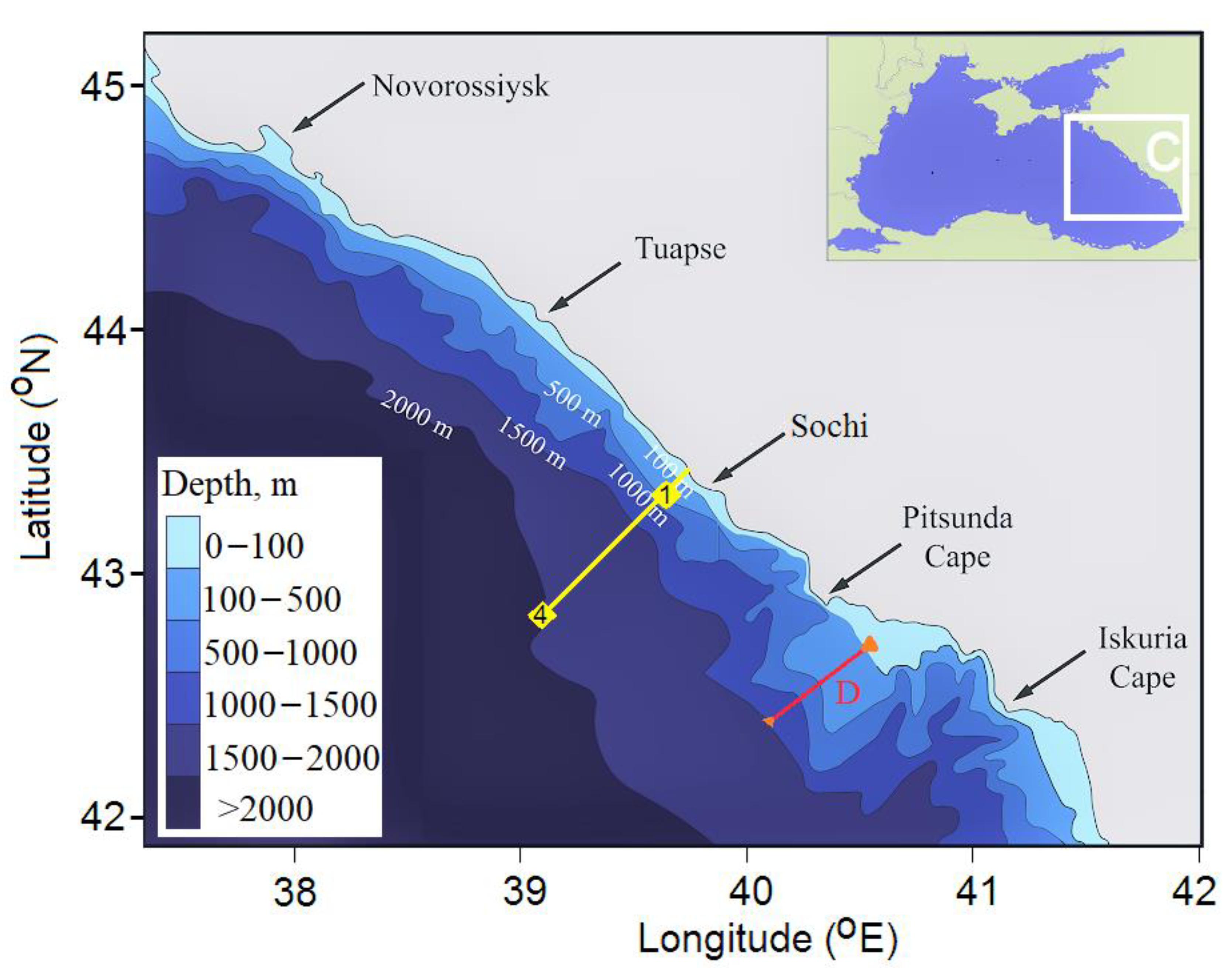
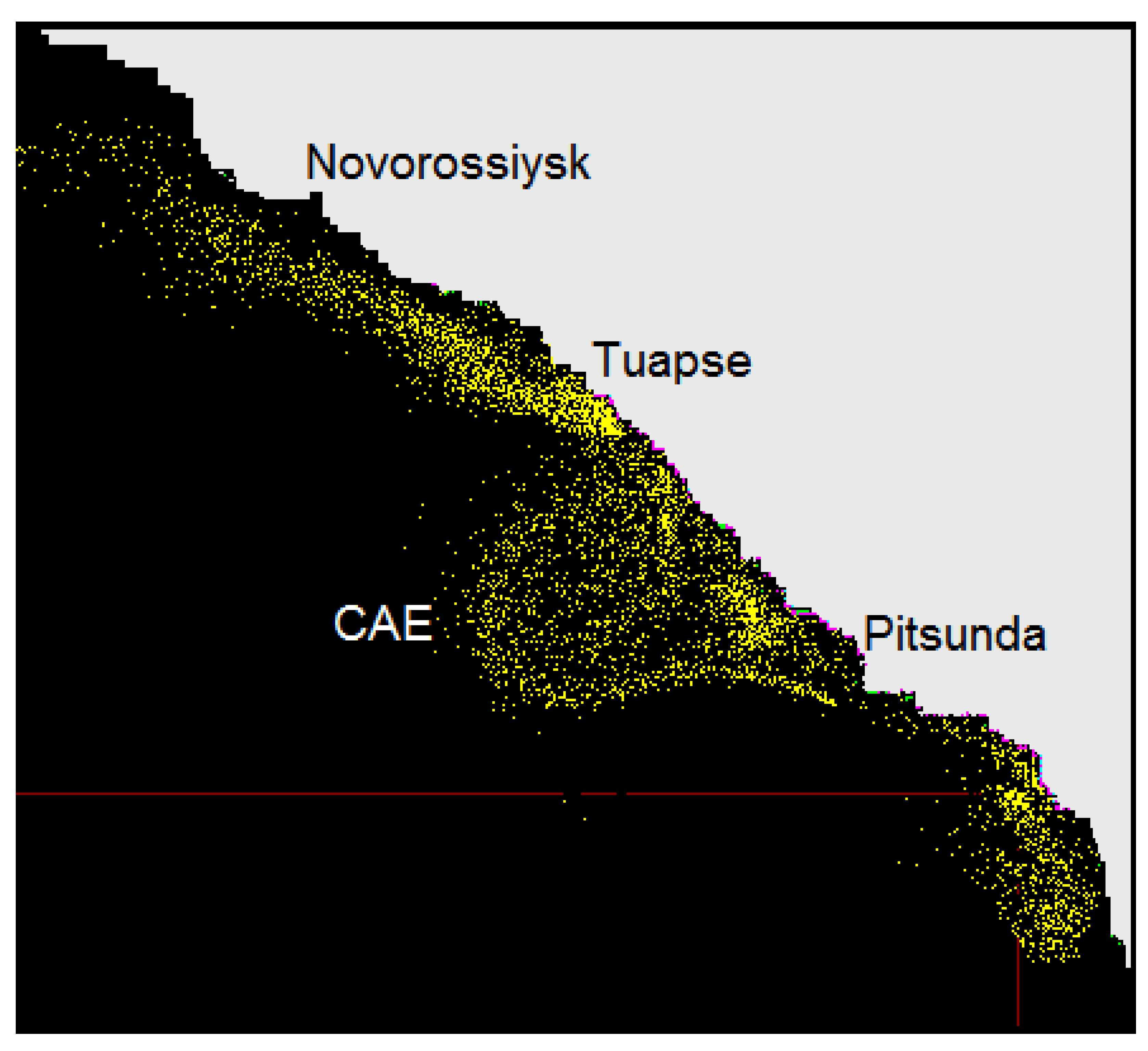
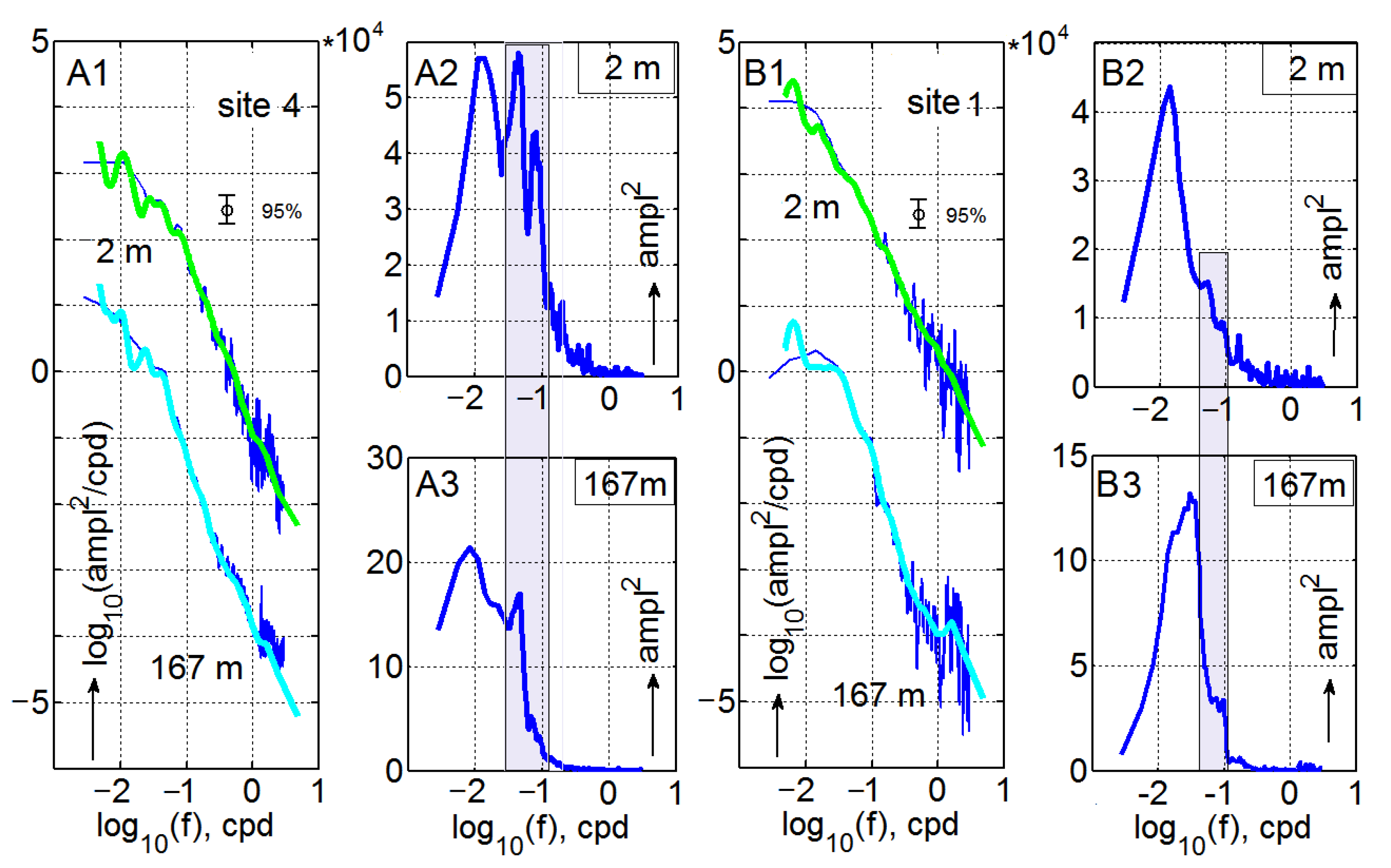
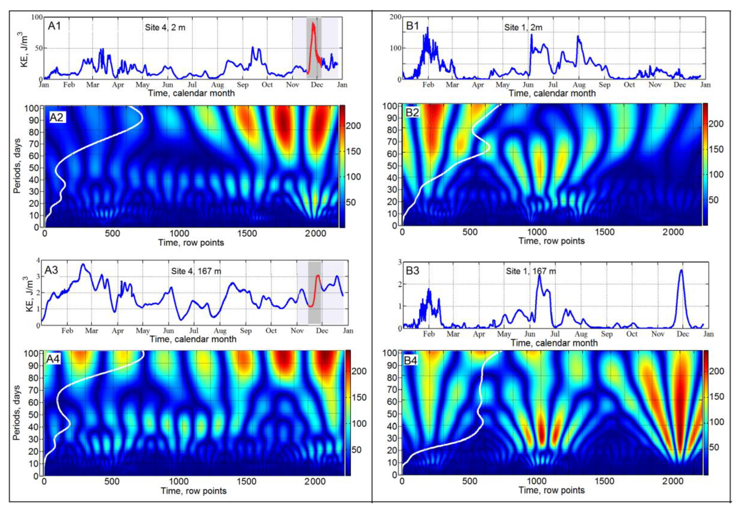
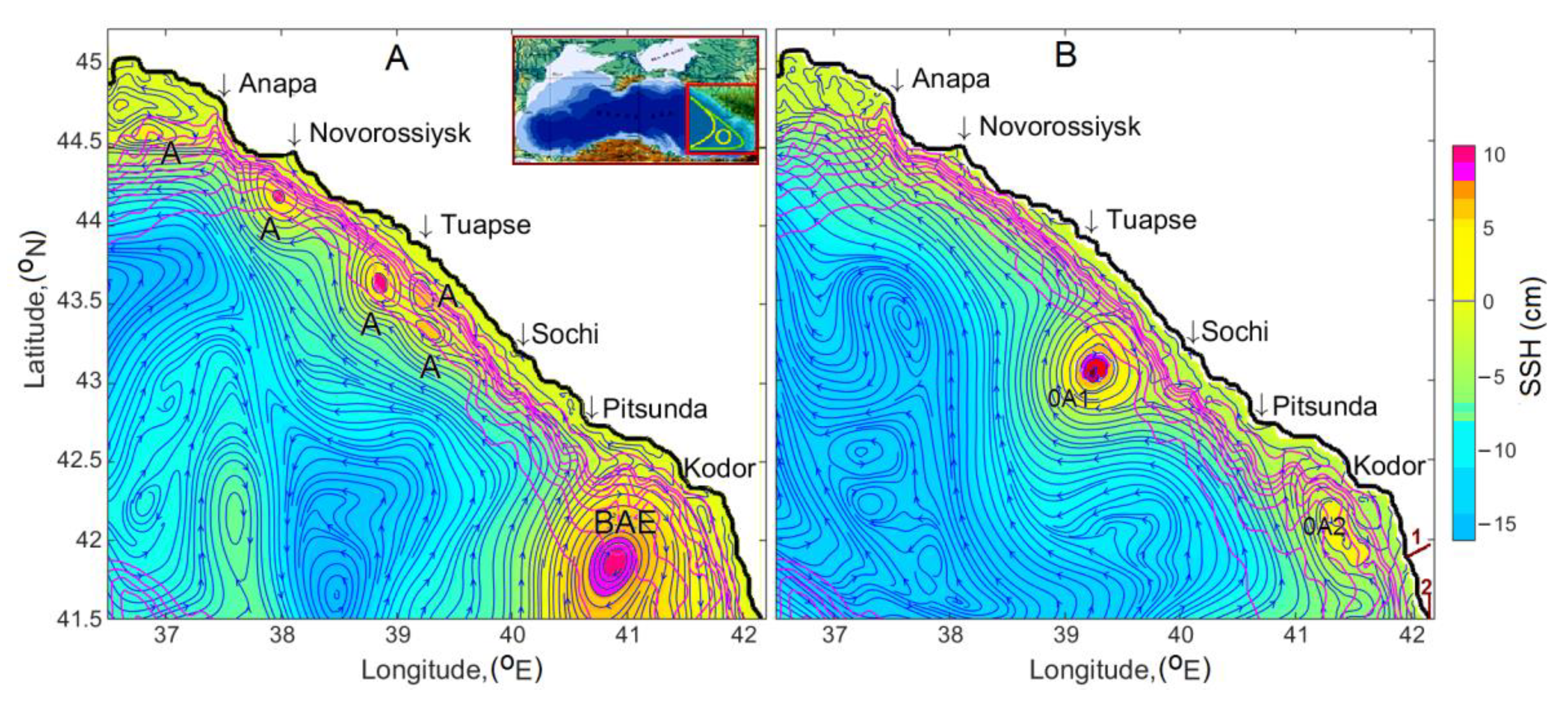
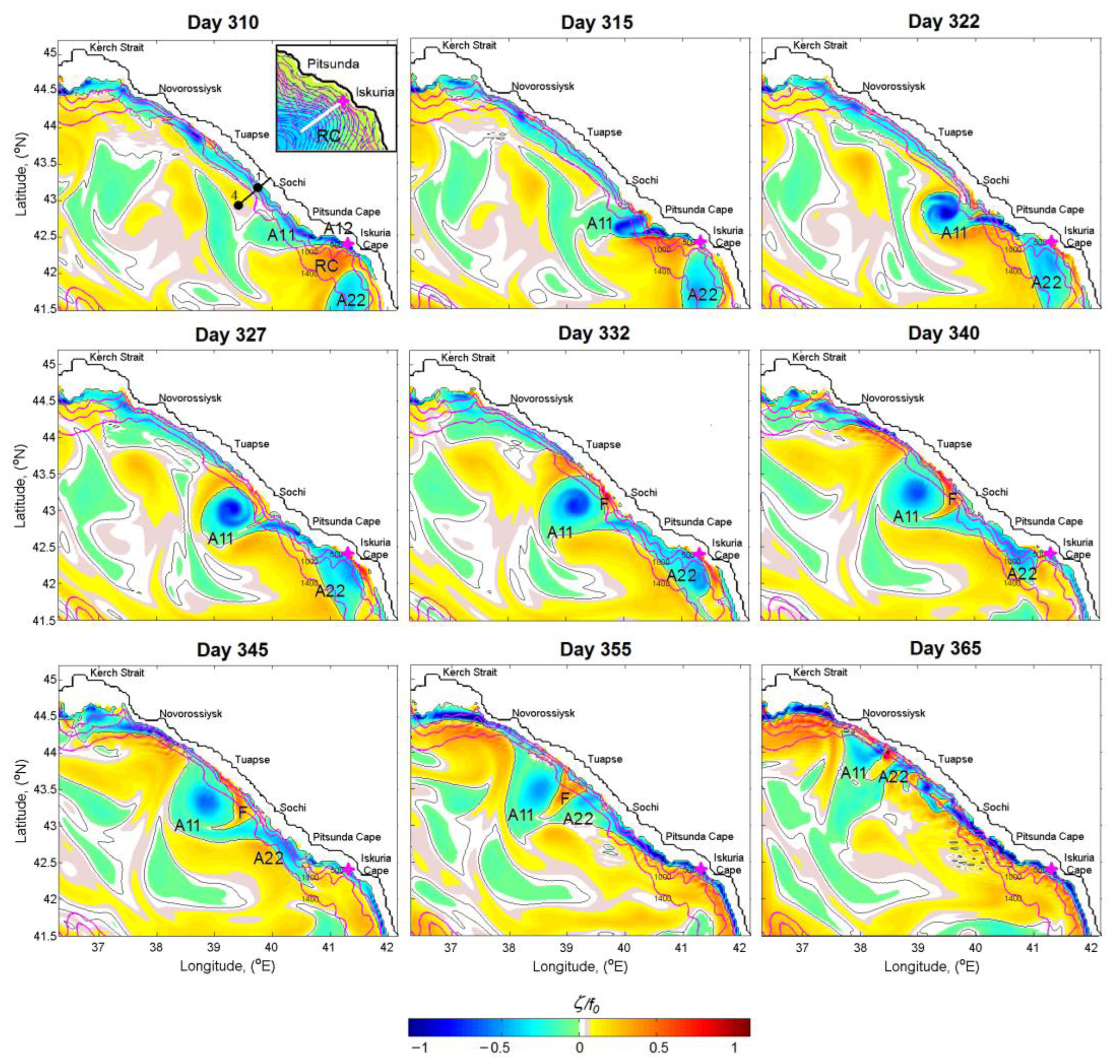
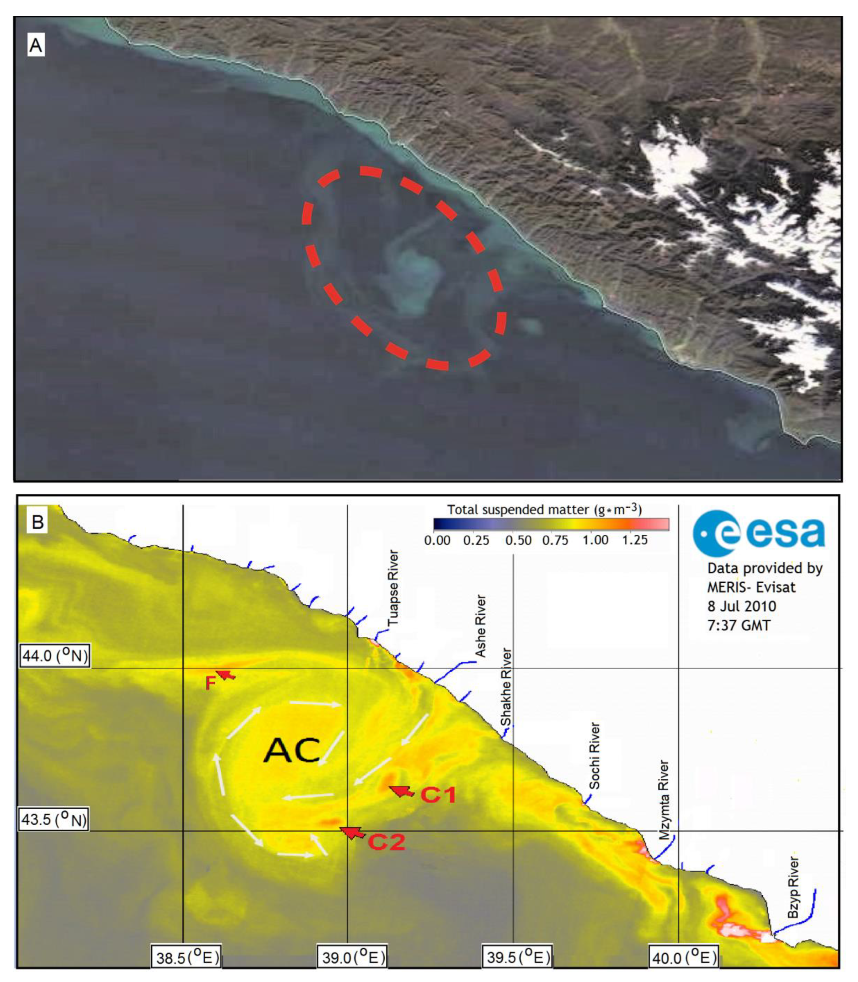
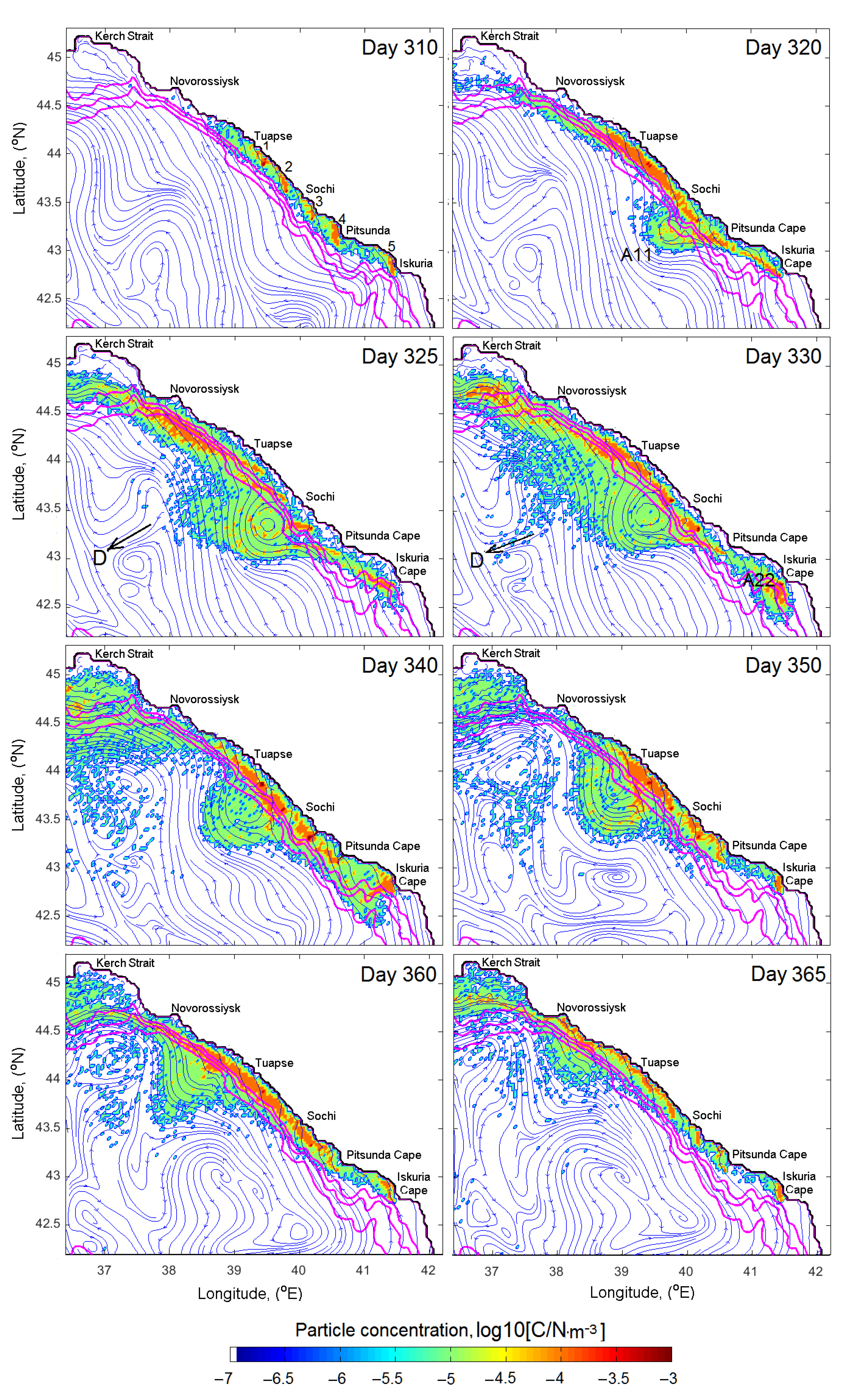
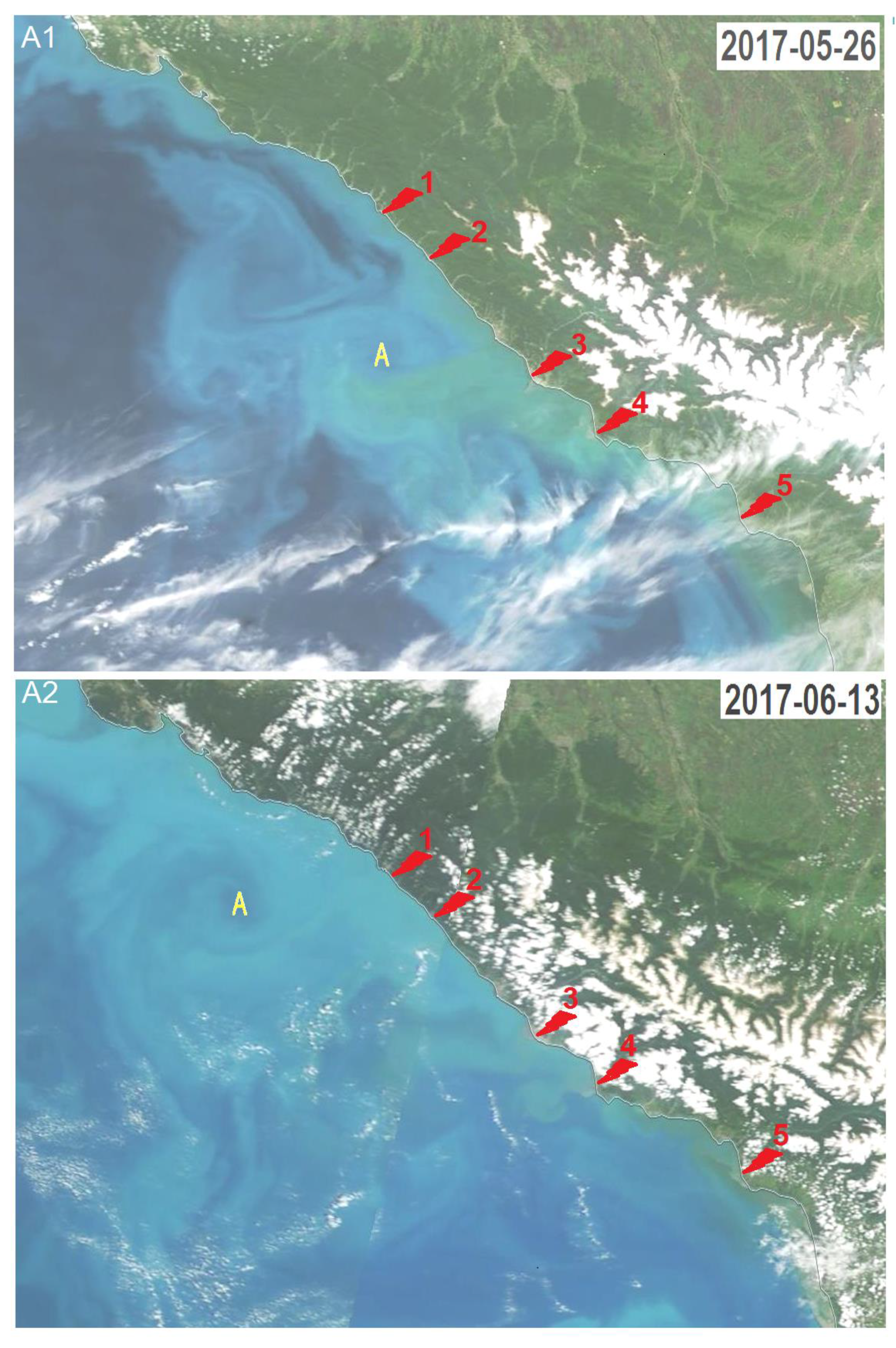
Table 1.
The normalized vertical vorticity ζ/f0 in eddies: Caucasian AE (A11), Batumi AE (A22), and at the site (A12).
Table 1.
The normalized vertical vorticity ζ/f0 in eddies: Caucasian AE (A11), Batumi AE (A22), and at the site (A12).
| Day | 305 | 310 | 315 | 322 | 327 | 332 | 340 | 345 | 355 | 365 |
|---|---|---|---|---|---|---|---|---|---|---|
| A11 | −0.0 | −0.9 | −1.2 | −0.8 | −0.8 | −0.6 | −0.6 | −0.6 | −0.4 | −0.2 |
| A12 | −1.0 | −0.6 | −0.3 | −0.4 | −0.4 | −0.80.4 | −0.2 | −0.4 | −0.5 | −0.6 |
| A22 | −0.4 | −0.4 | −0.4 | −0.3 | −0.3 | −0.3 | −0.2 | −0.2 | −0.1 | −0.1 |
Publisher’s Note: MDPI stays neutral with regard to jurisdictional claims in published maps and institutional affiliations. |
© 2022 by the authors. Licensee MDPI, Basel, Switzerland. This article is an open access article distributed under the terms and conditions of the Creative Commons Attribution (CC BY) license (https://creativecommons.org/licenses/by/4.0/).
Share and Cite
MDPI and ACS Style
Korotenko, K.; Osadchiev, A.; Melnikov, V. Mesoscale Eddies in the Black Sea and Their Impact on River Plumes: Numerical Modeling and Satellite Observations. Remote Sens. 2022, 14, 4149. https://doi.org/10.3390/rs14174149
AMA Style
Korotenko K, Osadchiev A, Melnikov V. Mesoscale Eddies in the Black Sea and Their Impact on River Plumes: Numerical Modeling and Satellite Observations. Remote Sensing. 2022; 14(17):4149. https://doi.org/10.3390/rs14174149
Chicago/Turabian StyleKorotenko, Konstantin, Alexander Osadchiev, and Vasiliy Melnikov. 2022. "Mesoscale Eddies in the Black Sea and Their Impact on River Plumes: Numerical Modeling and Satellite Observations" Remote Sensing 14, no. 17: 4149. https://doi.org/10.3390/rs14174149
Note that from the first issue of 2016, this journal uses article numbers instead of page numbers. See further details here.