Article

Global 10 m Land Use Land Cover Datasets: A Comparison of Dynamic World, World Cover and Esri Land Cover

1
Norwegian Institute for Nature Research—NINA, Sognsveien 68, 0855 Oslo, Norway
2
Atmospheric Sciences and Global Change Division, Pacific Northwest National Laboratory, Richland, WA 99352, USA
3
Geo-Ecological Research Group (GEco), Section for Research and Collections, Natural History Museum, The Faculty of Mathematics and Natural Sciences, University of Oslo, 0562 Oslo, Norway
4
School of Animal, Plant & Environmental Sciences, University of the Witwatersrand, Johannesburg 2000, South Africa
5
DST-NRF Centre of Excellence, Fitzpatrick Institute of African Ornithology, University of Cape Town, Rondebosch, Cape Town 7701, South Africa
*
Author to whom correspondence should be addressed.
Remote Sens. 2022, 14(16), 4101; https://doi.org/10.3390/rs14164101
Submission received: 22 July 2022 / Revised: 17 August 2022 / Accepted: 19 August 2022 / Published: 21 August 2022
(This article belongs to the Special Issue Remote Sensing of Land Use and Land Change with Google Earth Engine)

Abstract

:
The European Space Agency’s Sentinel satellites have laid the foundation for global land use land cover (LULC) mapping with unprecedented detail at 10 m resolution. We present a cross-comparison and accuracy assessment of Google’s Dynamic World (DW), ESA’s World Cover (WC) and Esri’s Land Cover (Esri) products for the first time in order to inform the adoption and application of these maps going forward. For the year 2020, the three global LULC maps show strong spatial correspondence (i.e., near-equal area estimates) for water, built area, trees and crop LULC classes. However, relative to one another, WC is biased towards over-estimating grass cover, Esri towards shrub and scrub cover and DW towards snow and ice. Using global ground truth data with a minimum mapping unit of 250 m2, we found that Esri had the highest overall accuracy (75%) compared to DW (72%) and WC (65%). Across all global maps, water was the most accurately mapped class (92%), followed by built area (83%), tree cover (81%) and crops (78%), particularly in biomes characterized by temperate and boreal forests. The classes with the lowest accuracies, particularly in the tundra biome, included shrub and scrub (47%), grass (34%), bare ground (57%) and flooded vegetation (53%). When using European ground truth data from LUCAS (Land Use/Cover Area Frame Survey) with a minimum mapping unit of <100 m2, we found that WC had the highest accuracy (71%) compared to DW (66%) and Esri (63%), highlighting the ability of WC to resolve landscape elements with more detail compared to DW and Esri. Although not analyzed in our study, we discuss the relative advantages of DW due to its frequent and near real-time data delivery of both categorical predictions and class probability scores. We recommend that the use of global LULC products should involve critical evaluation of their suitability with respect to the application purpose, such as aggregate changes in ecosystem accounting versus site-specific change detection in monitoring, considering trade-offs between thematic resolution, global versus. local accuracy, class-specific biases and whether change analysis is necessary. We also emphasize the importance of not estimating areas from pixel-counting alone but adopting best practices in design-based inference and area estimation that quantify uncertainty for a given study area.

1. Introduction

Global land use land cover (LULC) maps provide information necessary to quantify and understand Earth system processes and anthropogenic pressures, often at multiple spatial and temporal scales [1,2,3]. Earth observation and satellite remote sensing have enabled mapping LULC in a spatially explicit manner that ultimately informs policy and land management decisions aimed at achieving the global sustainable development goals [4]. Global LULC maps are adopted in a vast range of scientific domains and application environments. A few examples of LULC map application include: data input into mesoscale models for operational numerical weather forecasts and climate models for future climate projections [5,6]; outlining the extent of ecosystems and the change therein, e.g., as the basis for ecosystem service accounting [7,8]; isolating urban areas from their background to quantify local climate impacts [9]; informing spatial species distribution models that can predict and inform biodiversity conservation [10,11]; spatial conservation planning and environmental impact assessments [12]; monitoring deforestation and reporting to policy mechanisms, such as reduced emissions from deforestation and forest degradation (REDD+) [13]. One of the most impactful applications of global LULC maps going forward may be for ecosystem extent mapping following UN statistical standards for ecosystem accounting (EA) under the System of Environmental–Economic Accounting (SEEA) [14].
Over the past two decades, the spatial resolution of land cover maps has kept pace with the resolution of available satellite sensors, including the Moderate Resolution Imaging Spectroradiometer (MODIS; 250–500 m), PROBA-v (100 m) and Landsat (30 m) satellites. The most prominent corresponding global LULC maps include the National Aeronautics and Space Administration (NASA) MCD12Q1 500 m resolution dataset (2001–2018) [15], the European Space Agency (ESA) Copernicus Global Land Service (CGLS) Land Cover 100 m dataset (2015–2019) [16] and GlobLand30 (2010) [17]. While these products have been widely adopted, particularly at provincial to regional spatial scales, the medium spatial resolution prohibits the detection and monitoring of smaller landscape elements, which are vital to finer-scale Earth system processes and local land use planning. For instance, the monitoring and evaluation of agri-environmental schemes [18], such as installing hedge rows or semi-natural vegetation vital to pollinators, is not possible with the aforementioned LULC maps. Similarly, accounting for intra-urban blue–green space requires finer resolution data to distinguish street trees, green roofs and pocket parks from built surfaces [19].
Advancing upon the revolutionary legacy of the open-access Landsat missions [20], the European Space Agency (ESA) and Copernicus Programme have delivered globally consistent optical and radar data from the Sentinel satellites (10–20 m resolution) since 2014. Together with the advances in machine learning algorithms and cloud computing platforms for Earth observation, such as Google Earth Engine (GEE) [21] and openEO [22], the Sentinel satellites have enabled large-scale mapping of LULC at a 10 m resolution [2]. Since 2021, there have been three global Sentinel-based 10 m LULC maps released, including Google’s Dynamic World (DW) [23], ESA’s World Cover 2020 (WC) [24] and Esri’s 2020 Land Cover (Esri) [25]. All three products have the vision of being multi-temporal, with WC and Esri being annually updated, but only DW is operationally delivering near real-time LULC maps as new Sentinel-2 scenes become available (every 5 days). Esri and DW were both developed from deep learning models trained on the same reference dataset of over 5 billion hand-annotated Sentinel-2 pixel patches from 24,000 individual image tiles (510 × 510 pixels each) distributed over the world [23]. In contrast, WC was produced with a random forest classification tree algorithm trained on hand-labeled pixels in 100 × 100 m grids at 141,000 unique locations distributed over the world [24]. WC also included both Sentinel-1 and Sentinel-2 data as predictors in their model. Furthermore, a noteworthy difference is that the DW and Esri reference dataset was digitized with a minimum mapping unit (MMU) of 250 m2, while the WC reference dataset was digitized with an MMU of 100 m2.
To date, there have been no systematic evaluations of the three global 10 m LULC products with reference to one another. Given the importance of global LULC maps for various applications, and the large differences in the production of the recent 10 m products, we aimed to compare DW, WC and Esri global LULC maps in terms of their spatial correspondence with one another and their global and regional accuracy. To quantify accuracy at the global scale, we used the hand-annotated validation dataset published alongside DW. We supplemented this with a regional reference dataset of in situ point-based survey data on LULC across the European Union. We discuss how spatial correspondence and accuracy vary across LULC classes, biomes and human settlement types and explore key limitations and advantages of the three datasets.

2. Materials and Methods

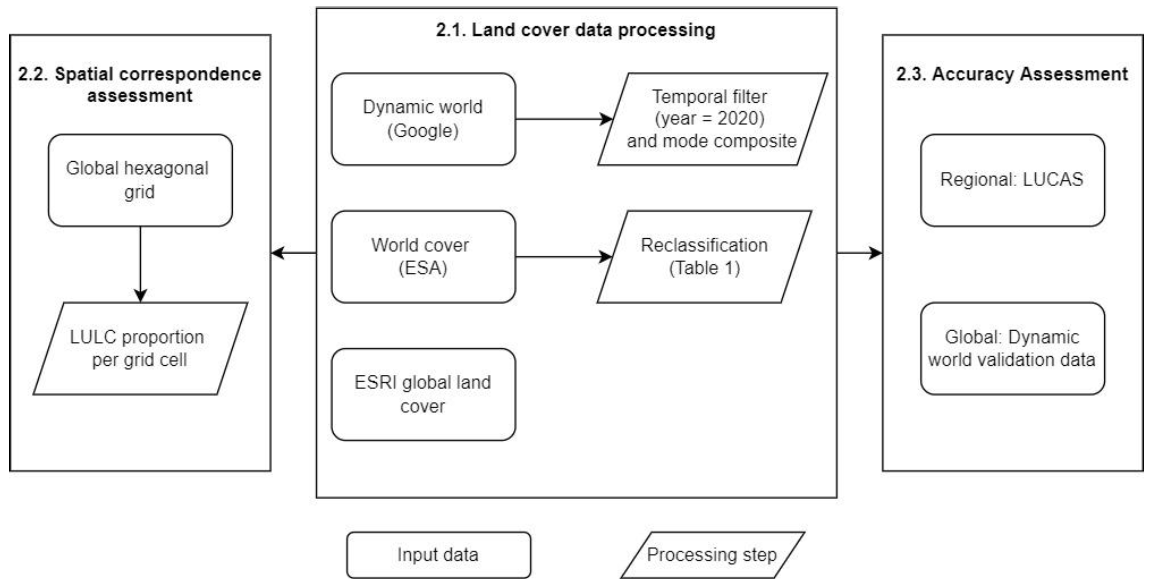
2.1. Land Cover Data Processing

Data pre-processing and extraction took place in GEE [21] and fed into our complete workflow, as outlined in Figure 1. Data analysis and visualization were performed in R [26]. The WC and Esri global land cover datasets for 2020 are available in the GEE official and community data catalogs. However, DW is provided as a collection of classified Sentinel-2 images with less than 35% cloud cover, as defined by the ‘CLOUDY_PIXEL_PERCENTAGE’ scene metadata property. Each image has a ‘label’ band with a discrete classification of LULC, but also 9 probability bands with class-specific probability scores generated by the deep learning model on the basis of the pixel’s spatial context. To generate an annual LULC composite comparable with WC and Esri, we calculated the mode of the predicted LULC class in the ‘label’ band of all DW images for 2020. We also tested annual compositing by calculating the mean and median probability scores for all LULC classes during the year and then classifying by taking the class with the highest probability score per pixel. We found no difference in overall accuracy using the alternative methods (Figure S1), and, because the mode composite on the ‘label’ band was more computationally efficient, we decided to use that global composite for further analysis. The land cover typologies were identical for DW and Esri; however, we converted the WC typology to match DW and Esri by aggregating four LULC classes, as outlined in Table 1. The three global 10 m LULC maps (Figure 2) were used to assess spatial correspondence and accuracy, as outlined below.

2.2. Spatial Correspondence Assessment

To assess how strongly the global LULC products corresponded to one another over space, we quantified and compared class-wise LULC area sums that were aggregated to an equal-area hexagonal grid (70,000 km2), which covered the globe. The size of the grid was chosen based on a trade-off between computation time and precision of area aggregation. Pixels were aggregated over mutually overlapping extents and image masks across the three LULC products. To quantify correspondence between products, for each LULC class and unique hexagonal grid cell, we calculate the proportional share of each product’s area estimation. Perfect correspondence resulted in a proportional ratio of 0.33:0.33:0.33 or 33% proportional share for each product. We defined strong correspondence when no single product’s proportional share of the LULC class area exceeded 40% in a grid cell. Therefore, weak correspondence was when the maximum difference between the product with the biggest and smallest proportional share was greater than 20%. We visualized these proportional shares for each hexagon over the globe by assigning a color code along a tri-color gradient using the tricolore (v1.2.2.) package in R. The relative abundance of the given LULC class (average of the three products’ area estimates) was mapped to the opacity of each hexagon grid so that areas where the LULC is abundant appear opaque and those where the LULC is less abundant are transparent.

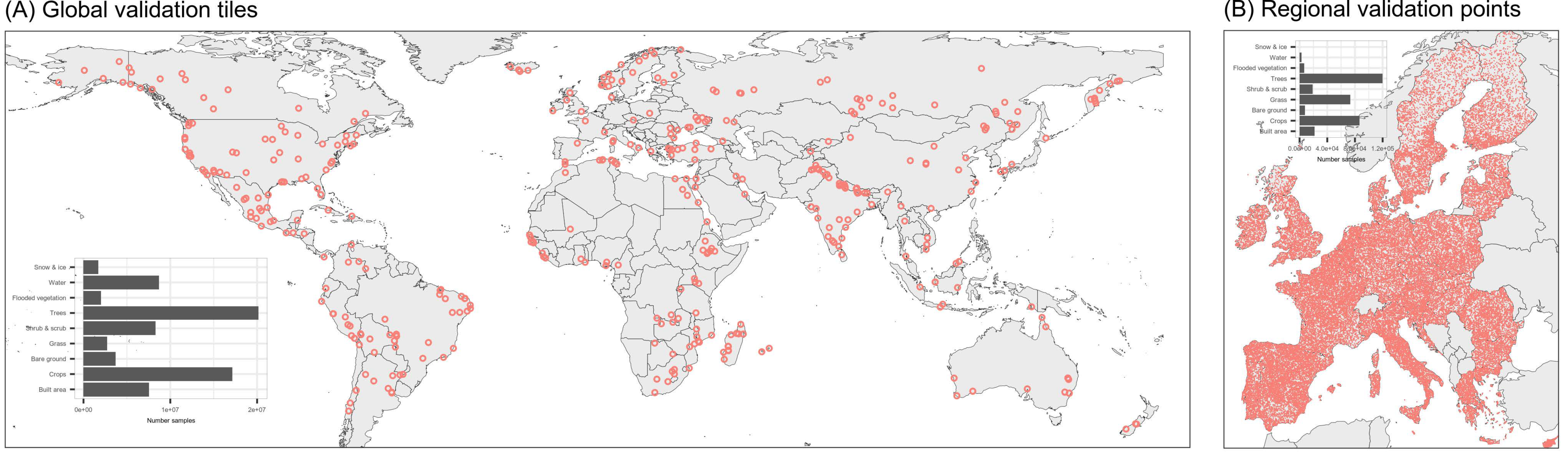
2.3. Accuracy Assessment

To quantify the accuracy of the three LULC products, we used two sources of open-access reference data (Figure 3). The first source was from the ground truth validation dataset produced by the Dynamic World team, which included a group of annotators (manual labeling of LULC types using visual interpretation of high-resolution reference imagery) supported by the National Geographic Society in partnership with Google and the World Resources Institute [23]. This team consisted of 25 expert and 45 non-expert annotators who together annotated approximately 24,000 individual image tiles of 510 × 510 pixels from Sentinel-2 imagery from random dates in 2019. Annotators followed the typology definitions outlined in the first column of Table 1 and were instructed to consider an MMU of 250 m2, which, by definition, included mosaics of distinct landscape elements within; for example, buildings, trees and grass within a 250 m2 area might be labeled as “built area”. From the annotated dataset, a stratified random subsample of 409 Sentinel-2 tiles were withheld from the training of the DW deep learning model and used for validation. The validation tiles included expert consensus labels where all three experts agreed, or where two experts agreed and the third had no opinion or where one expert had an opinion and the other two did not. We used this dataset constituting 72 million distinct 10 × 10 m pixels for global accuracy assessment of the three LULC products (Figure 3A). WC used a completely different reference dataset for training and validation of their model, which is not open-access, and, thus, we could not use it in the present analysis. Esri used the same reference dataset as DW to train and validate their LULC model; however, the sub-set of tiles they used for validating their map was not open-access, and, therefore, we cannot be sure that the 409 validation tiles we use here were in fact independent from the dataset used to train the Esri LULC model.
The second source of reference data was a regional dataset from the Land Use/Cover Area Frame Survey (LUCAS) over the European Union (Figure 3B). LUCAS is a systematic grid of 337,845 points that are visited triennially for the collection of in situ land cover and land use data [27]. In contrast to the DW ground truth dataset described above, LUCAS surveyors are instructed to record the land cover within a 1.5 m circle at each point in the grid, and, therefore, when applied to Earth observation, it consists of a significantly smaller MMU. We used the 2018 LUCAS dataset with the first-level classification with the exception of removing “G50: glaciers and permanent snow” from the water category into its own category to match the “snow and ice” category in the global LULC maps (Table 2).
The 2020 LULC predictions for each global product were sampled over the annotated image pixels (global validation set) and survey locations (regional validation set). Accuracy was quantified globally/regionally, but also stratified by biome, settlement type (urban, rural and uninhabited) and continent. Biomes were defined using the RESOLVE bioregions dataset [28], while human settlement type was derived from the Global Human Settlement Layers, Settlement Grid [29]. We constructed confusion matrices for each LULC product to calculate class-specific user’s/precision and producer’s/recall accuracy and overall accuracies.

2.4. Implementation Details

Data were summarized and/or extracted from GEE using the JavaScript API. The data were summarized by a global grid created using the dgggridR (v2.0.3) package. The figures were all created in R (v4.2.1) using the tricolore (v1.2.2.), ggplot2 (v3.3.5), ggmap (v3.0.0), sf (v1.0.9) and raster (v3.5) packages.

3. Results

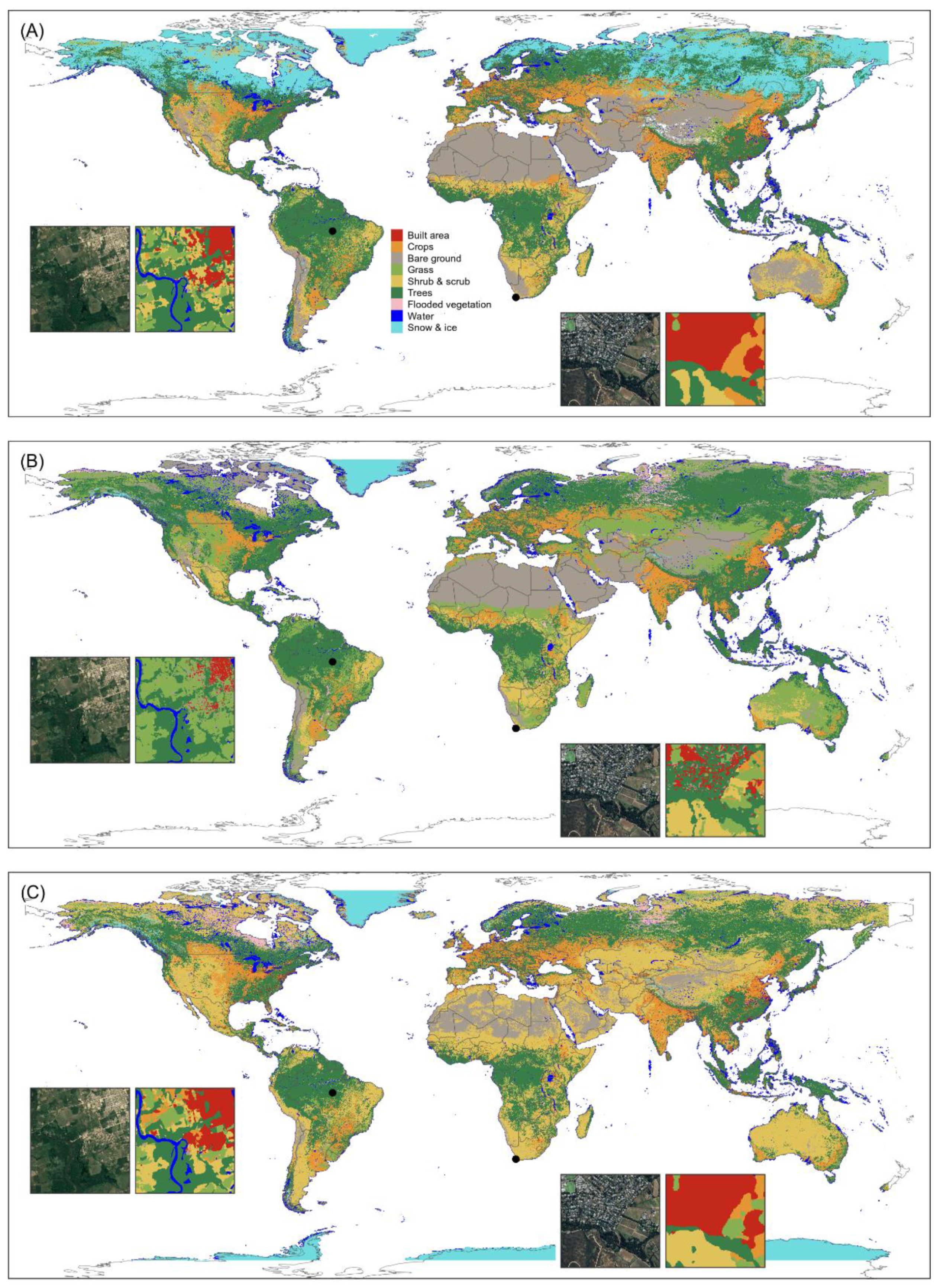
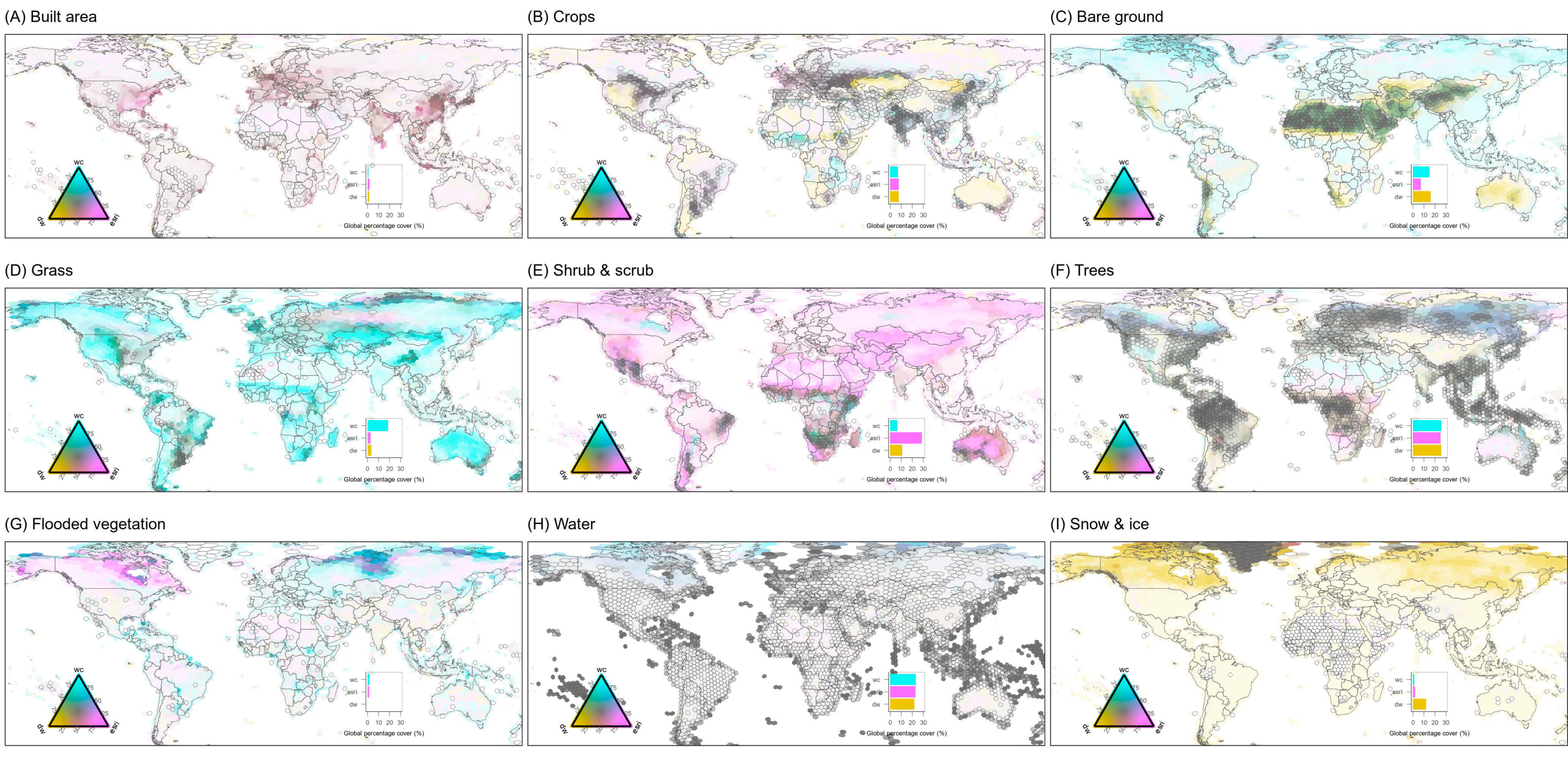
3.1. Spatial Correspondence
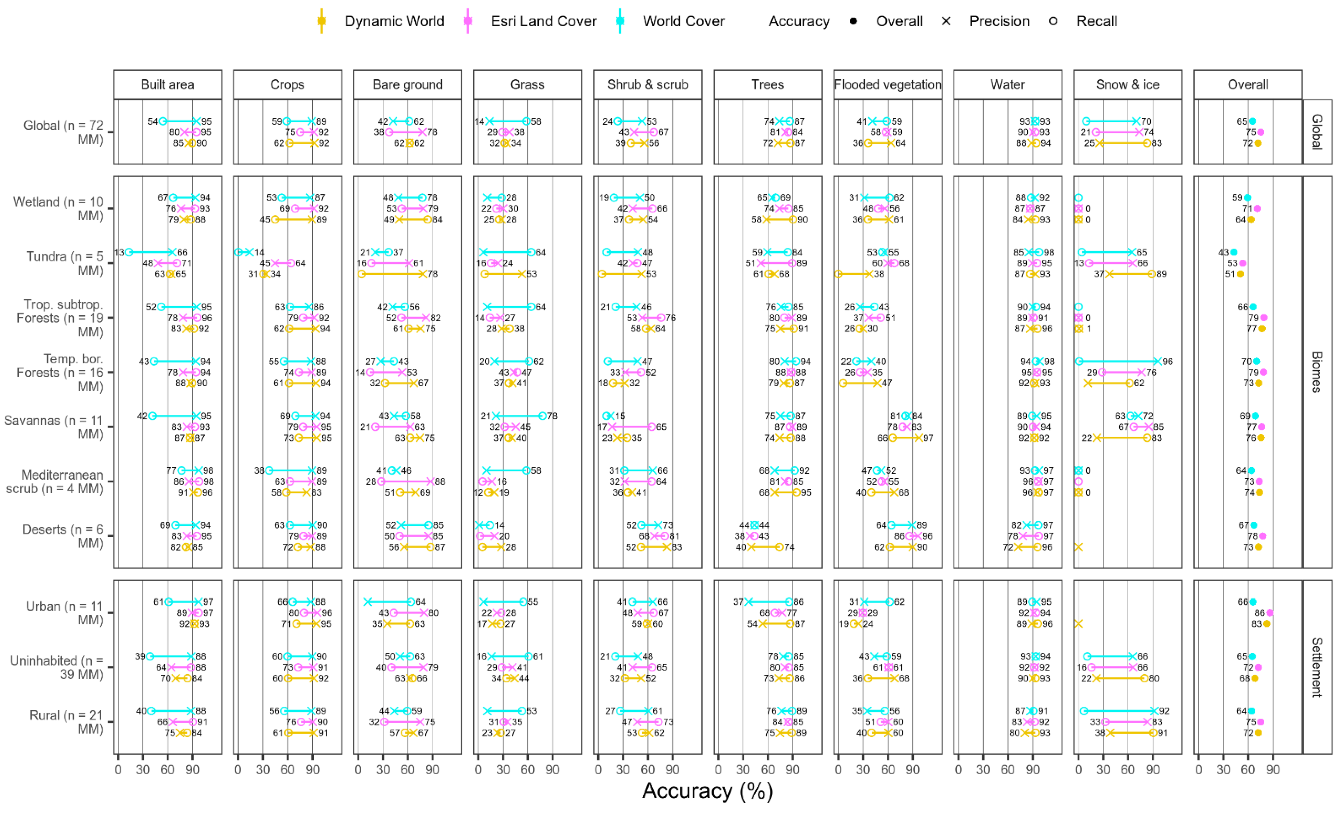
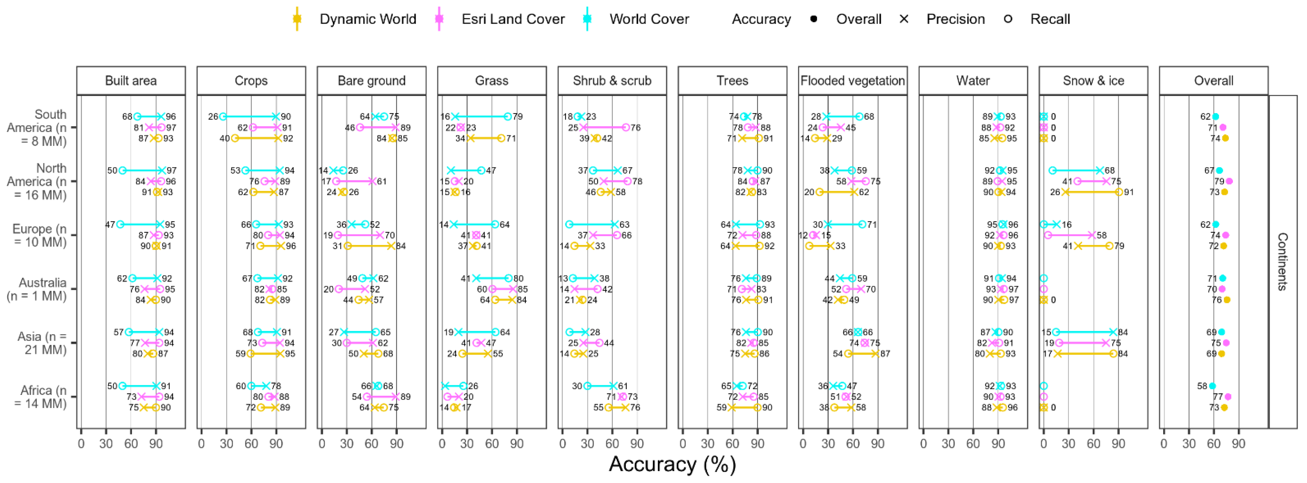
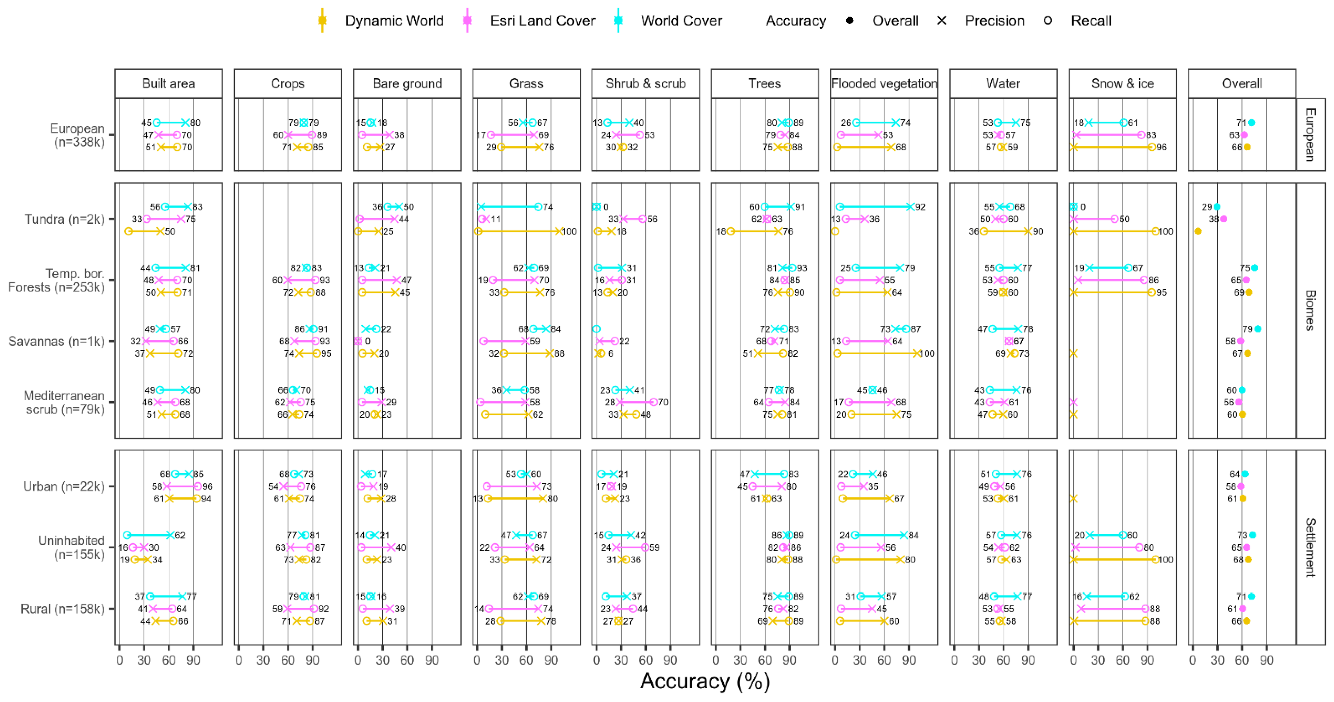
The area estimates for built area, crops, trees and water showed strong correspondence between the three global LULC products, particularly in areas with the greatest relative abundance of the given LULC class (i.e., gray areas with bordered grid cells in Figure 4). However, for some regions, there were discrepancies between products; for example, DW over-estimated the crop cover in the western USA, Kazakhstan and Mongolia relative to the other LULC products.
The LULC classes with the lowest correspondence between global products were bare ground, grass, scrub and shrub (Figure 4). DW estimated higher proportions of bare ground in mid- to lower latitudes, whereas WC estimated more bare ground in higher latitudes (Figure 4C). WC consistently estimated greater grass cover than DW and Esri across most of the world, except for over the taiga in Russia (Figure 4D). Conversely, the Esri product estimated greater shrub and scrub cover across the world except for a small section in Canada and the savanna-forest ecotone in central Africa (Figure 4E).
The LULC classes flooded vegetation, and snow and ice exhibited notable disagreements between products for the northern latitudes (Figure 4G,I). Esri estimated the highest proportions of flooded vegetation over North America, whereas WC estimated the highest proportions over Russia. DW estimated significantly more snow and ice cover than both WC and Esri over the whole of the Northern Hemisphere, apart from areas that are permanently snow-covered (e.g., Greenland) or snow-free (e.g., Sahara desert) (Figure 4I).

3.2. Accuracy

Using the global ground truth dataset with a minimum mapping unit of 250 m2, we found that Esri had the highest overall accuracy (75%) compared to DW (72%) and WC (65%; Table 3; Figure 5). Across all the LULC products, water was consistently the most accurately mapped class (balanced accuracy 92%; mean of precision and recall Figure 5), followed by built area (83%), trees (81%) and crops (78%). In contrast, bare ground (57%), grass (34%), shrub and scrub (47%) and flooded vegetation (53%) were mapped with the lowest accuracies (Figure 5). The accuracies across all the LULC products were generally lowest in the tundra biome, where grass, bare ground, shrub and scrub and crops were mis-classified and had the lowest recall and precision accuracies. The accuracies were the highest in temperate and boreal forests, where crops, trees and built area had the highest accuracies. There was very little difference in overall accuracy between urban, rural and uninhabited areas, with the exception that trees had lower precision in urban areas compared to rural and uninhabited areas, particularly for WC (40% lower) and DW (20% lower). Differences in accuracy between the continents were small; however, when averaged across LULC products, the accuracies were highest in North America and lowest in Africa (Figure 6).
Using the regional ground truth dataset (LUCAS) across Europe with an MMU of <100 m2, we found that the order of product accuracies was reversed compared to the global validation (Table 3; Figure 7). WC exhibited the highest accuracy (71%) compared to DW (66%) and Esri (63%). WC was particularly more accurate relative to DW and Esri in temporal and boreal forests and savanna biomes. Similar to the result from the global validation, the differences in accuracy between human settlement types were minimal. Furthermore, the relative differences in accuracy between LULC products were consistent across human settlement types. It should be noted that, for the European validation data, there were very few data points for the bare ground and snow and ice LULC classes, which may bias accuracy estimates significantly.

4. Discussion

4.1. Explaining the Differences between Global LULC Products

The production of global LULC maps is inherently difficult due to the extensive biogeographical variations within and across biomes that lead to diverse spectral signatures within a single LULC class [30]. In this sense, it is not surprising that three global LULC maps produced by three independent groups have large differences in accuracy and spatial correspondence. Below, we attempt to explain some of the main differences as presented in our results.

4.1.1. Minimum Mapping Unit

The global LULC maps had contrasting accuracies when validated against the global versus regional reference datasets (Figure 5 versus Figure 7). While Esri and DW were most accurate at the global scale, WC was most accurate at the European scale. Apart from the spatial extent, the most important difference between the reference datasets used to validate the LULC maps is the MMU used to collect ground truth information. The global validation dataset was digitized ex situ (i.e., based on visual interpretation of satellite imagery) using an MMU of 250 m2 (i.e., 50 × 50 m square), whereas the regional validation dataset (LUCAS) was collected in situ for point circles with a radius of 1.5 m (MMU <100 m). We suspect that the main reason Esri and DW had higher accuracies than WC at the global scale was because Esri and DW were produced from models trained on reference data with an MMU unit of 250 m2, while WC was trained on data with an MMU of 100 m2. We also posit that this difference in MMU is partially responsible for the difference in LULC classification granularity at the landscape scale. For instance, the inset maps in Figure 2 reveal how Esri and DW predictions are more clustered and generalized compared to WC, which exhibits more of the ‘salt and pepper’ characteristic of pixel-based classification techniques. Urban gardens and trees are incorporated into the “built area” cluster of pixels in DW and Esri maps, while they are labeled as “grass” or “trees” in WC. This illustrates why WC is 10% more accurate than Esri and DW when classifying built areas across Europe using the point-based LUCAS dataset as a reference (Figure 7).

4.1.2. Classification Typology

Another factor leading to differences between global LULC products is the classification typology used. For the purposes of cross-comparison, we harmonized all three LULC products to a nine-class typology (Table 1). Even though this is a much simpler typology than other regional LULC datasets (e.g., CORINE land cover [31]), there remain significant challenges in distinguishing spectrally similar classes, such as bare ground, grass, shrub and scrub, a finding often echoed in the literature [16,32,33]. These classes are not only difficult for satellite-based machine learning models to distinguish but also for human annotators using aerial or satellite imagery for visual interpretation. For instance, there was large disagreement between expert and non-expert labelers involved in developing the training dataset for DW and Esri [23]. A pixel-based comparison of expert and non-expert annotations revealed a recall rate (producer’s accuracy) as low as 22% for grass and 31% for bare ground. Although WC did not publish a similar uncertainty assessment of its annotation team, it is reasonable to assume their reference dataset suffered from the same error. It is known that, even with in situ LULC labeling (i.e., field-based ground truth), similar errors due to sampler bias may exist. For instance, the European Environment Agency discovered that CORINE-2000 accuracy was boosted by 6.4% following post-screening and cleaning of erroneous LULC labels in the LUCAS dataset [34]. This partly explains why the spatial correspondence between global LULC products and class-level accuracy was generally poorest for bare ground, grass and shrub and scrub cover (Figure 4 and Figure 5).
Another source of discrepancy between LULC products is the slight difference in LULC definitions for certain classes (see descriptions in Table 1). For instance, the flooded vegetation class in DW and Esri includes rice paddies and irrigated/inundated agriculture. In WC, this type of cropland is included in the cropland class. Furthermore, the DW reference dataset defines the shrub and scrub class relatively broadly as clusters of plants that are dispersed over an area without any specification of cover percentage (“…moderate to sparse cover of bushes, shrubs, and tufts of grass”) [23]. This is different to the WC typology, where grass, bare ground and shrub/scrub are defined using specific cover percentages (“…shrubs having a cover of 10% or more. Shrubs are defined as woody perennial plants with persistent and woody stems and without any defined main stem being less than 5 m tall”) [24].

4.1.3. Modeling and Validation Methods

At the global scale, the accuracies of DW, WC and Esri were different to one another (Figure 5) and also different to the independent accuracies reported by the data providers themselves: DW 72% versus reported 74%; WC 65% versus reported 74%; Esri 75% versus 85%. The discrepancy for DW is likely due to the fact that we aggregated LULC predictions to an annual composite for 2020 (using the mode of the ‘label’ band), whereas the DW validation report used scene-level model predictions for Sentinel-2 tiles in 2019. The WC dataset was produced and validated with a completely different reference dataset with a different MMU to the DW validation tiles used here. The metadata published with the Esri dataset is incomplete, and, thus, we do not know which reference data were withheld from model training and whether the 409 validation tiles used here were indeed independent from the Esri training dataset. If it is the case that the validation data used here had been part of the data used to train the Esri deep learning model, then it is possible that our estimates of the Esri map accuracy are overly optimistic.
The DW and Esri maps were produced using a deep learning model, whereas WC was produced using a random forest classification. This difference in modeling framework likely explains some of the difference in accuracy between LULC products. Deep learning models, such as the fully convolutional neural network employed in DW, take the pixel context into account when making inferences, whereas random forest does not. This, together with the difference in MMU, explains why the DW and Esri maps are clustered and generalized at a landscape scale (inset maps Figure 2).
Finally, we acknowledge that we are using reference data from 2019 (global) and 2018 (European) that do not align with the year of the LULC maps (2020) and that this may lead to discrepancies between the validation set and the reality on the ground in 2020. However, we suspect these changes to be minimal, and any bias introduced should be consistent across global LULC products. Furthermore, even the WC reference dataset, which is not open-access, faces the same limitation as it was collected for the year 2015 and used to create and validate the WC map for the year 2020.

4.2. Recommendations for Users

The cross-comparison results presented here indicate that there is no “one-size-fits-all” when it comes to global LULC maps and their potential application. We find differences in accuracy across spatial scales (global versus regional), LULC classes, continents, biomes and urban settlement types. Therefore, an overall recommendation is to carefully evaluate the global LULC products with respect to the aforementioned factors and how they relate to the application requirements. We note that it is also possible to use all three LULC products in combination by creating some form of majority vote or weighted average. Nevertheless, we make some general recommendations for users of either DW, Esri or WC or a combination thereof:
  • Regardless of LULC product, users should implement design-based inference when calculating LULC areas or changes and avoid drawing conclusions from simple ‘pixel-counting’, which leads to biased area estimates [35]. Design-based inference involves generating a post-classification reference (validation or “ground truth”) sample that is implemented with a probability sampling design (e.g., simple random or stratified random), which can be used to quantify unbiased area and accuracy estimates.
  • In general, users can rely on water, built area, trees and crops being mapped with the highest accuracy, while shrub and scrub, grass, bare ground and flooded vegetation have the lowest accuracies. With this in mind, it may be beneficial to simplify the LULC typology by merging classes with low accuracies into aggregate classes if your use-case allows it.
  • Users should be aware of the biases in global LULC products (reported relative to one another). Specifically, WC is biased toward estimating greater grass cover, Esri towards shrub and scrub cover and DW towards snow and ice.
  • LULC classification accuracy varies by biome, continent and urban settlement type, and, therefore, users may consult Figure 4, Figure 5 and Figure 6 here to gather information on what to expect given the local context of their work.
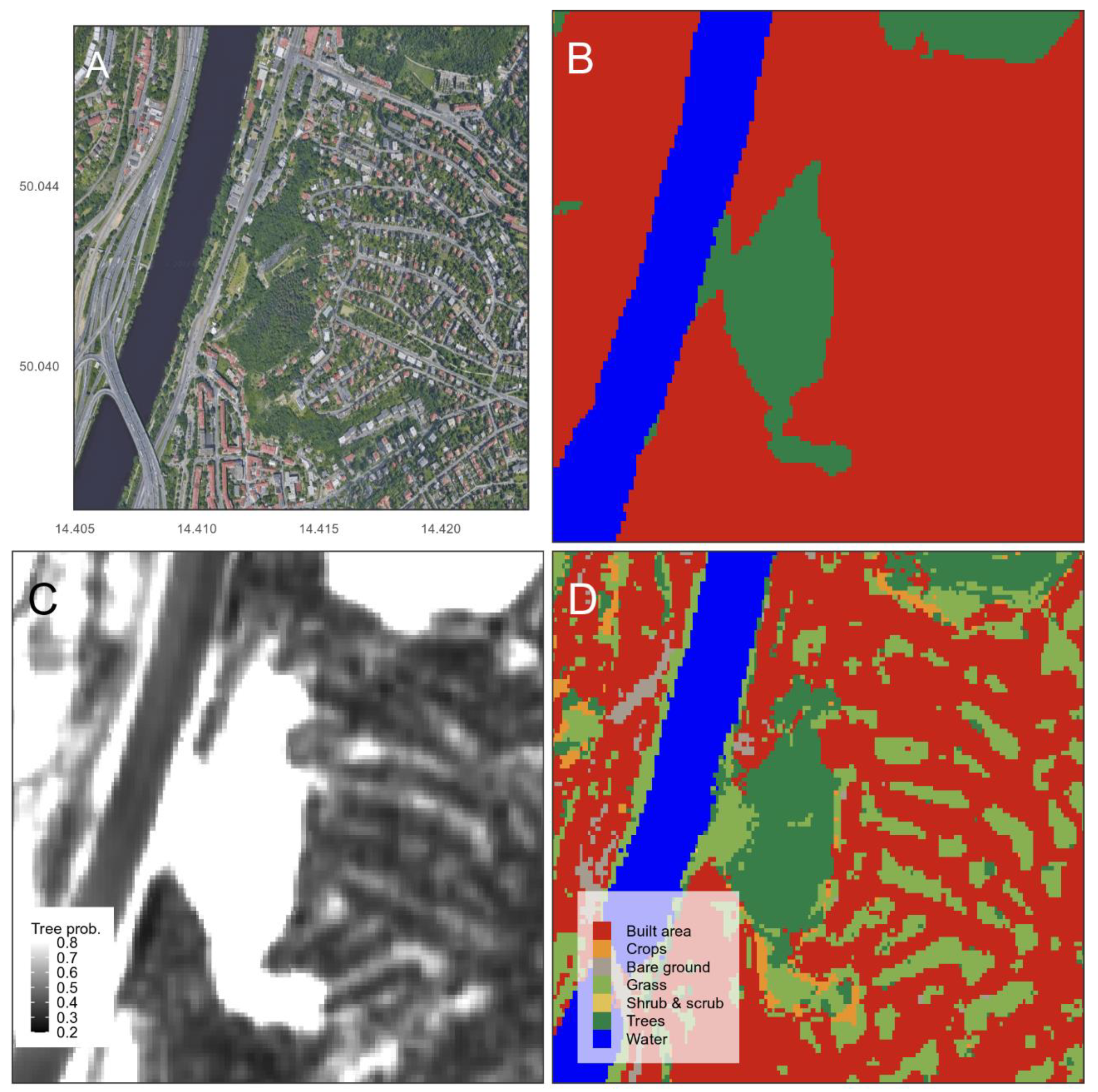
  • WC is most appropriate when considering an MMU of <100 m2 or when a user wants to resolve smaller landscape elements. For example, WC is advantageous in urban areas and complex agricultural landscapes with small or thin vegetation structures, such as trees or hedge rows.
  • Based on our supplementary analysis of the DW compositing method (Figure S1), we find that the type of temporal aggregation of DW predictions has very little effect on global and regional accuracy. However, we note that changing the seasonal extent of temporal aggregation (e.g., growing-season composite) may have significant effects on accuracy (although we did not test this here).
  • The delivery format of DW in near real-time, covering the entire Sentinel-2 image collection and including LULC class-specific probability scores, is qualitatively unique from Esri and WC, which only produce annual LULC maps without probability scores. We encourage users to take advantage of this unique aspect to DW by exploring novel possibilities discussed in the section below.

4.3. Potential for Future Research

Although our analysis provides important information about global model accuracies, it remains to be seen which LULC product provides area change estimates with the least amount of error as measured using design-based inference for area estimation [35,36]. Quantifying confidence intervals around area estimates or area change estimates is necessary for the adoption of LULC products in policy mechanisms, such as the REDD+ [13] reporting on deforestation or the SEEA ecosystem accounting [14]. It is, therefore, of interest to test DW, Esri and WC (as well as other multi-temporal medium resolution maps (e.g., Friedl et al., 2022 [37]) in terms of how accurately they estimate changes in LULC at various spatial and temporal scales. However, design-based inference can be time-consuming and costly. A requirement for design-based inference is an explicitly specified population, and, in the context of evaluating map accuracy, this population often refers to a population of pixels included in a map and given different class labels. This population varies spatially and temporally depending on the project scope, and, therefore, a probability-based sample needs to be generated for making an inference each time the project scope changes. The probability scores provided by DW may allow for more efficient alternatives to design-based inference. Sales et al., 2021 [38] have shown that averaging class probability scores from a random forest model can give area estimates that are substantially less biased than ‘pixel-counting’ and almost as precise as design-based methods. The same might be true of DW class probability scores. Furthermore, there is also scope to use DW probability scores to estimate per-pixel classification accuracy [39,40].
The probability scores available in the DW product provide scope for several other avenues of further research and tailored LULC classification. Firstly, they can be aggregated over time frames relevant to the application task. For example, annual composites might be appropriate for some tasks, while summer or winter mosaics might be appropriate for others. Secondly, users can apply custom thresholds or more complex decision frameworks to the predicted probabilities in order to derive continuous or discrete LULC outputs (Figure 8C). For example, this type of thresholding can be used to generate surface water extent data much more frequently than the global surface water (GSW) dataset without any update lags (currently up to 18 months). Thirdly, users can train their own local machine learning models using DW probability scores and custom reference data as the input (Figure 8D). This may allow for changing the LULC typology or resolving finer-scale landscape elements that are not present in the default DW ‘label’ band. Users that explore custom models, such as DNN architectures, may also try different loss functions that result in predictions that are less clustered and able to resolve finer details. For example, Lang et al., 2022 [41] use GEDI reference data at 25 m but produce a tree canopy height model at a 10 m resolution. Fourthly, frequency and near real-time availability of the class probability scores allow for application of advanced time series analysis, such as LandTrendr (Landsat-based detection of trends in disturbance and recovery) and CCDC (continuous change detection and classification) [42].
There are several spheres of application for which 10 m LULC maps are particularly well-suited. Urban ecology and climate science is one such area because landscape composition and structure often manifest at scales of 10 m or less. In an increasingly urbanizing planet, it is important to accurately monitor global and regional urban extent for planning purposes. How these newer-generation datasets compare to existing estimates across regions is still largely unknown [43]. There is also potential for using DW to quantify seasonal land cover dynamics (e.g., including urban vegetation phenology [44]) within cities, which is not possible with static annual LULC maps. The spatial compositions of LULC and LULC changes are important for modeling landscape connectivity and biodiversity community dynamics [45]. Urban ecology may, therefore, benefit from comparing the landscape metrics that result from global 10 m LULC maps.
Ecosystem accounting is another application where multi-temporal 10 m LULC maps may prove particularly useful. Many have highlighted the need for remote-sensing-based approaches to implement ecosystem extent-condition accounting in ecosystem services mapping for ecosystem accounts [46]. A challenge for ecosystem accounting has been that biophysical mapping of ecosystem services at a national level has relied on discrete categories of land cover types typical of traditional LULC maps. Therefore, ecosystem service models have not been sensitive to transitional or successional changes from one LULC type to another typical of ecological gradients or continuums [47]. It is possible that DW probability scores can detect continuous gradients in ecosystem accounting and that LULC probability can be thought of as a higher-level structural composition indicator within the ecosystem condition typology. Area-weighted probabilities have been computed for biodiversity indices but typically at much coarser spatial levels [48]. It is possible that LULC class probabilities could be applied to some standard ecosystem services (required by EUROSTAT) in decreasing order of accuracy, including (i) biomass, carbon storage and sequestration, air filtration, run-off control; (ii) somewhat less for local climate regulation and landscape aesthetics/greenview exposure and (iii) even less for crop pollination and recreation potential. Therefore, class probability scores could allow a merging of the extent-condition account for the purpose of more accurate ecosystem service computation (i.e., reducing the information loss in using threshold levels for classifying LULC types for the extent account on its own—moving from Figure 8C to Figure 8D).

5. Conclusions

LULC mapping at global extents has been revolutionized by the plethora of medium-resolution satellite data available from programs such as Landsat and Sentinel. In our cross-comparison of global 10 m resolution LULC maps, we found large inaccuracies and spatial and thematic biases in each product that vary across biomes, continents and human settlement types. Our overarching recommendation is to critically evaluate each LULC product with reference to the application purpose. We highlight the novelty of DW as a global near real-time LULC product with class probability scores. LULC types, regardless of definition and type system, share with ecosystems the property that their composition, structure and processes often vary in a gradual, continuous manner over space and time. We suggest that the DW probability scores offer a fundamental shift in land cover mapping from categorical to continuum concepts.

Supplementary Materials

The following supporting information can be downloaded at: https://www.mdpi.com/article/10.3390/rs14164101/s1, Figure S1: Accuracy of three types of annual compositing of Dynamic World land cover maps at the global and regional extent. Compositing methods include a model reducer on the label band, and a mean and median reducer on the class probabilities, followed by a highest probability vote classification. Global validation is based on hand-annotated image tiles with a minimum mapping unit of 50 × 50 m. European validation is based on point-based ground truth data from the LUCAS survey. Accuracy is expressed as precision/user’s, recall/producer’s and overall accuracy based on a confusion matrix with sample sizes indicated in thousands (K) in parenthesis on the y-axis.

Author Contributions

Conceptualization, Z.S.V.; methodology, Z.S.V. and G.S.; formal analysis, Z.S.V.; writing—original draft preparation, Z.S.V.; writing—review and editing, D.N.B., T.S., T.C. and G.S.; funding acquisition, D.N.B. All authors have read and agreed to the published version of the manuscript.

Funding

This paper was funded by Norwegian Research Council grant number 320042 and the APC was funded by Norwegian Research Council.

Institutional Review Board Statement

Not applicable.

Informed Consent Statement

Not applicable.

Data Availability Statement

The code and data to reproduce this analysis have been archived here: https://github.com/NINAnor/GlobalLULCcompare, accessed on 21 July 2022.

Acknowledgments

This paper was supported by the EcoGaps project funded by Norwegian Research Council grant number 320042. The Pacific Northwest National Laboratory (PNNL) is operated for DOE by Battelle Memorial Institute under contract DE-AC05-76RLO1830.

Conflicts of Interest

The authors declare no conflict of interest.

References

  1. Chaves, M.E.D.; Picoli, M.C.A.; Sanches, I.D. Recent Applications of Landsat 8/OLI and Sentinel-2/MSI for Land Use and Land Cover Mapping: A Systematic Review. Remote Sens. 2020, 12, 3062. [Google Scholar] [CrossRef]
  2. Phiri, D.; Simwanda, M.; Salekin, S.; Nyirenda, V.R.; Murayama, Y.; Ranagalage, M. Sentinel-2 Data for Land Cover/Use Mapping: A Review. Remote Sens. 2020, 12, 2291. [Google Scholar] [CrossRef]
  3. Liu, L.; Zhang, X.; Gao, Y.; Chen, X.; Shuai, X.; Mi, J. Finer-Resolution Mapping of Global Land Cover: Recent Developments, Consistency Analysis, and Prospects. J. Remote Sens. 2021, 2021, 5289697. [Google Scholar] [CrossRef]
  4. Kavvada, A.; Metternicht, G.; Kerblat, F.; Mudau, N.; Haldorson, M.; Laldaparsad, S.; Friedl, L.; Held, A.; Chuvieco, E. Towards Delivering on the Sustainable Development Goals Using Earth Observations. Remote Sens. Environ. 2020, 247, 111930. [Google Scholar] [CrossRef]
  5. Lawrence, P.J.; Chase, T.N. Representing a New MODIS Consistent Land Surface in the Community Land Model (CLM 3.0). J. Geophys. Res. Biogeosci. 2007, 112, G01023. [Google Scholar] [CrossRef]
  6. Kurkowski, N.P.; Stensrud, D.J.; Baldwin, M.E. Assessment of Implementing Satellite-Derived Land Cover Data in the Eta Model. Weather Forecast. 2003, 18, 404–416. [Google Scholar] [CrossRef] [Green Version]
  7. Andrew, M.E.; Wulder, M.A.; Nelson, T.A. Potential Contributions of Remote Sensing to Ecosystem Service Assessments. Prog. Phys. Geogr. Earth Environ. 2014, 38, 328–353. [Google Scholar] [CrossRef] [Green Version]
  8. Martínez-Harms, M.J.; Balvanera, P. Methods for Mapping Ecosystem Service Supply: A Review. Int. J. Biodivers. Sci. Ecosyst. Serv. Manag. 2012, 8, 17–25. [Google Scholar] [CrossRef]
  9. Chakraborty, T.; Sarangi, C.; Lee, X. Reduction in Human Activity Can Enhance the Urban Heat Island: Insights from the COVID-19 Lockdown. Environ. Res. Lett. 2021, 16, 054060. [Google Scholar] [CrossRef]
  10. Randin, C.F.; Ashcroft, M.B.; Bolliger, J.; Cavender-Bares, J.; Coops, N.C.; Dullinger, S.; Dirnböck, T.; Eckert, S.; Ellis, E.; Fernández, N.; et al. Monitoring Biodiversity in the Anthropocene Using Remote Sensing in Species Distribution Models. Remote Sens. Environ. 2020, 239, 111626. [Google Scholar] [CrossRef]
  11. Sydenham, M.A.K.; Venter, Z.S.; Eldegard, K.; Moe, S.R.; Steinert, M.; Staverløkk, A.; Dahle, S.; Skoog, D.I.J.; Hanevik, K.A.; Skrindo, A.; et al. High Resolution Prediction Maps of Solitary Bee Diversity Can Guide Conservation Measures. Landsc. Urban Plan. 2022, 217, 104267. [Google Scholar] [CrossRef]
  12. Hersperger, A.M.; Grădinaru, S.R.; Pierri Daunt, A.B.; Imhof, C.S.; Fan, P. Landscape Ecological Concepts in Planning: Review of Recent Developments. Landsc. Ecol. 2021, 36, 2329–2345. [Google Scholar] [CrossRef] [PubMed]
  13. Gao, Y.; Skutsch, M.; Paneque-Gálvez, J.; Ghilardi, A. Remote Sensing of Forest Degradation: A Review. Environ. Res. Lett. 2020, 15, 103001. [Google Scholar] [CrossRef]
  14. Edens, B.; Maes, J.; Hein, L.; Obst, C.; Siikamaki, J.; Schenau, S.; Javorsek, M.; Chow, J.; Chan, J.Y.; Steurer, A.; et al. Establishing the SEEA Ecosystem Accounting as a Global Standard. Ecosyst. Serv. 2022, 54, 101413. [Google Scholar] [CrossRef]
  15. Sulla-Menashe, D.; Gray, J.M.; Abercrombie, S.P.; Friedl, M.A. Hierarchical Mapping of Annual Global Land Cover 2001 to Present: The MODIS Collection 6 Land Cover Product. Remote Sens. Environ. 2019, 222, 183–194. [Google Scholar] [CrossRef]
  16. Buchhorn, M.; Lesiv, M.; Tsendbazar, N.-E.; Herold, M.; Bertels, L.; Smets, B. Copernicus Global Land Cover Layers—Collection 2. Remote Sens. 2020, 12, 1044. [Google Scholar] [CrossRef] [Green Version]
  17. Chen, J.; Chen, J.; Liao, A.; Cao, X.; Chen, L.; Chen, X.; He, C.; Han, G.; Peng, S.; Lu, M.; et al. Global Land Cover Mapping at 30 m Resolution: A POK-Based Operational Approach. ISPRS J. Photogramm. Remote Sens. 2015, 103, 7–27. [Google Scholar] [CrossRef] [Green Version]
  18. Cole, L.J.; Kleijn, D.; Dicks, L.V.; Stout, J.C.; Potts, S.G.; Albrecht, M.; Balzan, M.V.; Bartomeus, I.; Bebeli, P.J.; Bevk, D.; et al. A Critical Analysis of the Potential for EU Common Agricultural Policy Measures to Support Wild Pollinators on Farmland. J. Appl. Ecol. 2020, 57, 681–694. [Google Scholar] [CrossRef]
  19. Hanssen, F.; Barton, D.; Cimburova, Z. Mapping Urban Tree Canopy Cover Using Airborne Laser Scanning—Applications to Urban Ecosystem Accounting for Oslo; NINA Report: Trondheim, Norway, 2019. [Google Scholar]
  20. Zhu, Z.; Wulder, M.A.; Roy, D.P.; Woodcock, C.E.; Hansen, M.C.; Radeloff, V.C.; Healey, S.P.; Schaaf, C.; Hostert, P.; Strobl, P. Benefits of the Free and Open Landsat Data Policy. Remote Sens. Environ. 2019, 224, 382–385. [Google Scholar] [CrossRef]
  21. Gorelick, N.; Hancher, M.; Dixon, M.; Ilyushchenko, S.; Thau, D.; Moore, R. Google Earth Engine: Planetary-Scale Geospatial Analysis for Everyone. Remote Sens. Environ. 2017, 202, 18–27. [Google Scholar] [CrossRef]
  22. Schramm, M.; Pebesma, E.; Milenković, M.; Foresta, L.; Dries, J.; Jacob, A.; Wagner, W.; Mohr, M.; Neteler, M.; Kadunc, M.; et al. The OpenEO API–Harmonising the Use of Earth Observation Cloud Services Using Virtual Data Cube Functionalities. Remote Sens. 2021, 13, 1125. [Google Scholar] [CrossRef]
  23. Brown, C.F.; Brumby, S.P.; Guzder-Williams, B.; Birch, T.; Hyde, S.B.; Mazzariello, J.; Czerwinski, W.; Pasquarella, V.J.; Haertel, R.; Ilyushchenko, S.; et al. Dynamic World, Near Real-Time Global 10 m Land Use Land Cover Mapping. Sci. Data 2022, 9, 251. [Google Scholar] [CrossRef]
  24. Zanaga, D.; Van De Kerchove, R.; De Keersmaecker, W.; Souverijns, N.; Brockmann, C.; Quast, R.; Wevers, J.; Grosu, A.; Paccini, A.; Vergnaud, S.; et al. ESA WorldCover 10 m 2020 V100. OpenAIRE 2021. [Google Scholar] [CrossRef]
  25. Karra, K.; Kontgis, C.; Statman-Weil, Z.; Mazzariello, J.C.; Mathis, M.; Brumby, S.P. Global Land Use/Land Cover with Sentinel 2 and Deep Learning; IEEE: Manhattan, NY, USA, 2021; pp. 4704–4707. [Google Scholar]
  26. R Core Team. R: A Language and Environment for Statistical Computing 2021. R Foundation for Statistical Computing, Vienna, Austria. Available online: https://www.R-project.org/ (accessed on 21 July 2022).
  27. D’Andrimont, R.; Yordanov, M.; Martinez-Sanchez, L.; Eiselt, B.; Palmieri, A.; Dominici, P.; Gallego, J.; Reuter, H.I.; Joebges, C.; Lemoine, G.; et al. Harmonised LUCAS In-Situ Land Cover and Use Database for Field Surveys from 2006 to 2018 in the European Union. Sci. Data 2020, 7, 352. [Google Scholar] [CrossRef]
  28. Dinerstein, E.; Olson, D.; Joshi, A.; Vynne, C.; Burgess, N.D.; Wikramanayake, E.; Hahn, N.; Palminteri, S.; Hedao, P.; Noss, R. An Ecoregion-Based Approach to Protecting Half the Terrestrial Realm. BioScience 2017, 67, 534–545. [Google Scholar] [CrossRef] [PubMed]
  29. Pesaresi, M.; Freire, S. GHS Settlement Grid Following the REGIO Model 2014 in Application to GHSL Landsat and CIESIN GPW V4-Multitemporal (1975–1990–2000–2015). JRC Data Cat. 2016. Available online: http://data.europa.eu/89h/jrc-ghsl-ghs_smod_pop_globe_r2016a (accessed on 21 July 2022).
  30. Halvorsen, R.; Skarpaas, O.; Bryn, A.; Bratli, H.; Erikstad, L.; Simensen, T.; Lieungh, E. Towards a Systematics of Ecodiversity: The EcoSyst Framework. Glob. Ecol. Biogeogr. 2020, 29, 1887–1906. [Google Scholar] [CrossRef]
  31. Büttner, G. CORINE Land Cover and Land Cover Change Products. In Land Use and Land Cover Mapping in Europe; Springer: Berlin/Heidelberg, Germany, 2014; pp. 55–74. [Google Scholar]
  32. Venter, Z.S.; Sydenham, M.A.K. Continental-Scale Land Cover Mapping at 10 m Resolution Over Europe (ELC10). Remote Sens. 2021, 13, 2301. [Google Scholar] [CrossRef]
  33. Pflugmacher, D.; Rabe, A.; Peters, M.; Hostert, P. Mapping Pan-European Land Cover Using Landsat Spectral-Temporal Metrics and the European LUCAS Survey. Remote Sens. Environ. 2019, 221, 583–595. [Google Scholar] [CrossRef]
  34. Büttner, G.; Maucha, G. The Thematic Accuracy of Corine Land Cover 2000. Assessment Using LUCAS (Land Use/Cover Area Frame Statistical Survey). Eur. Environ. Agency Cph. Den. 2006, 7, 1–85. [Google Scholar]
  35. Olofsson, P.; Foody, G.M.; Herold, M.; Stehman, S.V.; Woodcock, C.E.; Wulder, M.A. Good Practices for Estimating Area and Assessing Accuracy of Land Change. Remote Sens. Environ. 2014, 148, 42–57. [Google Scholar] [CrossRef]
  36. Stehman, S.V.; Foody, G.M. Key Issues in Rigorous Accuracy Assessment of Land Cover Products. Remote Sens. Environ. 2019, 231, 111199. [Google Scholar] [CrossRef]
  37. Friedl, M.A.; Woodcock, C.E.; Olofsson, P.; Zhu, Z.; Loveland, T.; Stanimirova, R.; Arevalo, P.; Bullock, E.; Hu, K.-T.; Zhang, Y.; et al. Medium Spatial Resolution Mapping of Global Land Cover and Land Cover Change Across Multiple Decades From Landsat. Front. Remote Sens. 2022, 3, 894571. [Google Scholar] [CrossRef]
  38. Sales, M.H.; De Bruin, S.; Souza, C.; Herold, M. Land Use and Land Cover Area Estimates from Class Membership Probability of a Random Forest Classification. IEEE Trans. Geosci. Remote Sens. 2021, 60, 1–11. [Google Scholar] [CrossRef]
  39. Khatami, R.; Mountrakis, G.; Stehman, S.V. Predicting Individual Pixel Error in Remote Sensing Soft Classification. Remote Sens. Environ. 2017, 199, 401–414. [Google Scholar] [CrossRef]
  40. Ebrahimy, H.; Mirbagheri, B.; Matkan, A.A.; Azadbakht, M. Per-Pixel Land Cover Accuracy Prediction: A Random Forest-Based Method with Limited Reference Sample Data. ISPRS J. Photogramm. Remote Sens. 2021, 172, 17–27. [Google Scholar] [CrossRef]
  41. Lang, N.; Jetz, W.; Schindler, K.; Wegner, J.D. A High-Resolution Canopy Height Model of the Earth. arXiv 2022, arXiv:2204.08322. [Google Scholar]
  42. Pasquarella, V.J.; Arévalo, P.; Bratley, K.H.; Bullock, E.L.; Gorelick, N.; Yang, Z.; Kennedy, R.E. Demystifying LandTrendr and CCDC Temporal Segmentation. Int. J. Appl. Earth Obs. Geoinf. 2022, 110, 102806. [Google Scholar] [CrossRef]
  43. Potere, D.; Schneider, A. A Critical Look at Representations of Urban Areas in Global Maps. GeoJournal 2007, 69, 55–80. [Google Scholar] [CrossRef]
  44. Meng, L.; Mao, J.; Zhou, Y.; Richardson, A.D.; Lee, X.; Thornton, P.E.; Ricciuto, D.M.; Li, X.; Dai, Y.; Shi, X. Urban Warming Advances Spring Phenology but Reduces the Response of Phenology to Temperature in the Conterminous United States. Proc. Natl. Acad. Sci. USA 2020, 117, 4228–4233. [Google Scholar] [CrossRef]
  45. Uroy, L.; Alignier, A.; Mony, C.; Foltête, J.-C.; Ernoult, A. How to Assess the Temporal Dynamics of Landscape Connectivity in Ever-Changing Landscapes: A Literature Review. Landsc. Ecol. 2021, 36, 2487–2504. [Google Scholar] [CrossRef]
  46. Notte, A.L.; Czúcz, B.; Vallecillo, S.; Polce, C.; Maes, J. Ecosystem Condition Underpins the Generation of Ecosystem Services: An Accounting Perspective. One Ecosyst. 2022, 7, e81487. [Google Scholar] [CrossRef]
  47. McGill, B.J. Towards a Unification of Unified Theories of Biodiversity. Ecol. Lett. 2010, 13, 627–642. [Google Scholar] [CrossRef]
  48. Jakobsson, S.; Töpper, J.P.; Evju, M.; Framstad, E.; Lyngstad, A.; Pedersen, B.; Sickel, H.; Sverdrup-Thygeson, A.; Vandvik, V.; Velle, L.G. Setting Reference Levels and Limits for Good Ecological Condition in Terrestrial Ecosystems–Insights from a Case Study Based on the IBECA Approach. Ecol. Indic. 2020, 116, 106492. [Google Scholar] [CrossRef]
Figure 1. Flowchart of the methods followed in the cross-comparison and accuracy assessment of global 10 m LULC maps.
Remotesensing 14 04101 g001
Figure 2. Maps of global 10 m resolution land cover maps, including Dynamic World (A), World Cover (B) and Esri Land Cover (C). Inset maps show a zoomed extent of a landscape in South Africa and Brazil, indicated with black dots on the world maps to illustrate the spatial grain of the maps at a local scale. White areas in the Arctic and Antarctic in (A,B), although partly mapped in (C), were not included in the analysis.
Remotesensing 14 04101 g002
Figure 3. Distribution of the global (A) and regional (B) reference data locations. Locations in (A) represent Sentinel-2 image tiles of 510 × 510 pixels, which were manually annotated ex situ. Locations in (B) are grid points sampled in situ in the LUCAS area survey. Inset bar plot shows the number of reference samples per LULC class.
Remotesensing 14 04101 g003
Figure 4. Spatial correspondence between global 10 m land cover maps for each of 9 land cover classes. The proportion of land cover within each hexagonal grid cell is calculated for each LULC product and then visualized along a tri-color gradient illustrating the proportional share of areas estimated by each LULC product. Gray areas indicate strong correspondence, whereas colored areas reflect dominance of one LULC product. Gric cells outlined in black indicate strong correspondence, defined as cases where no single LULC product has more than 40% share of the combined area within the grid cell. The opacity of the grid cells indicates the absolute percentage abundance of each LULC class averaged over the three LULC classes. Opaque areas have near-maximum percentage cover for that LULC class, whereas transparent areas have very low percentage cover.
Remotesensing 14 04101 g004
Figure 5. Accuracy of global 10 m land cover maps across LULC classes, biomes and human settlement type based on hand-annotated image tiles with minimum mapping unit of 50 × 50 m. Accuracy is expressed as precision/user’s, recall/producer’s and overall accuracy based on a confusion matrix, with sample sizes indicated in millions (MM) in parentheses on the y-axis.
Remotesensing 14 04101 g005
Figure 6. Accuracy of global 10 m land cover maps across LULC classes and continents based on hand-annotated image tiles with MMU unit of 50 × 50 m. Circles show users, producers and overall accuracy. Accuracy is expressed as precision/user’s, recall/producer’s and overall accuracy based on a confusion matrix, with sample sizes indicated in millions (MM) in parentheses on the y-axis.
Remotesensing 14 04101 g006
Figure 7. Accuracy of global 10 m land cover maps over Europe using point-based ground truth data from the LUCAS survey. Accuracy is stratified by LULC class, ecoregion and human settlement type. Accuracy is expressed as precision/user’s, recall/producer’s and overall accuracy based on a confusion matrix, with sample sizes indicated in thousands (K) in parentheses on the y-axis.
Remotesensing 14 04101 g007
Figure 8. Example of the flexibility inherent in the Dynamic World data format, which includes multi-temporal class probability estimates. An urban landscape in Prague, Czechia (A) along with an annual mode composite from Dynamic World (B). Dynamic World class probabilities for the tree class are rescaled to highlight intra-urban tree cover (C). The predictions from a random forest model trained on LUCAS reference data and Dynamic World class probabilities are shown in (D), illustrating the possibility of resolving smaller landscape elements.
Remotesensing 14 04101 g008
Table 1. Classification typology cross-walk between the three global 10 m LULC maps included in this study.
Dynamic WorldEsri LULCWorld Cover
Built AreaBuilt AreaBuilt-up
Clusters of human-made structures or individual very large human-made structures. Contained industrial, commercial and private building and the associated parking lots. A mixture of residential buildings, streets, lawns, trees, isolated residential structures or buildings surrounded by vegetative land cover. Major road and rail networks outside of the predominant residential areas. Large homogeneous impervious surfaces, including parking structures, large office buildings and residential housing developments containing clusters of cul-de-sacs.Human-made structures; major road and rail networks; large homogenous impervious surfaces, including parking structures, office buildings and residential housing; examples: houses, dense villages/towns/cities, paved roads, asphalt.Land covered by buildings, roads and other man-made structures, such as railroads. Buildings include both residential and industrial buildings. Urban green (parks, sport facilities) is not included in this class. Waste dump deposits and extraction sites are considered as bare.
CropsCropsCropland
Human planted/plotted cereals, grasses and crops.Human planted/plotted cereals, grasses and crops not at tree height; examples: corn, wheat, soy, fallow plots of structured land.Land covered with annual cropland that is sowed/planted and harvestable at least once within the 12 months after the sowing/planting date. The annual cropland produces a herbaceous cover and is sometimes combined with some tree or woody vegetation. Note that perennial woody crops will be classified as the appropriate tree cover or shrub land cover type. Greenhouses are considered as built-up.
Bare groundBare groundBarren/sparse vegetation
Areas of rock or soil containing very sparse to no vegetation. Large areas of sand and deserts with no to little vegetation. Large individual or dense networks of dirt roads.Areas of rock or soil with very sparse to no vegetation for the entire year; large areas of sand and deserts with no to little vegetation; examples: exposed rock or soil, desert and sand dunes, dry salt flats/pans, dried lake beds, mines.Lands with exposed soil, sand or rocks and never has more than 10 % vegetated cover during any time of the year.
Moss and Lichen
Land covered with lichens and/or mosses. Lichens are composite organisms formed from the symbiotic association of fungi and algae. Mosses contain photo-autotrophic land plants without true leaves, stems, roots but with leaf- and stemlike organs.
GrassGrassGrassland
Open areas covered in homogenous grasses with little to no taller vegetation. Other homogenous areas of grass-like vegetation (blade-type leaves) that appear different from trees and shrubland. Wild cereals and grasses with no obvious human plotting (i.e., not a structured field).Open areas covered in homogenous grasses with little to no taller vegetation; wild cereals and grasses with no obvious human plotting (i.e., not a plotted field); examples: natural meadows and fields with sparse to no tree cover, open savanna with few to no trees, parks/golf courses/lawns, pastures.This class includes any geographic area dominated by natural herbaceous plants (plants without persistent stem or shoots above ground and lacking definite firm structure): (grasslands, prairies, steppes, savannahs, pastures) with a cover of 10% or more, irrespective of different human and/or animal activities, such as: grazing, selective fire management, etc. Woody plants (trees and/or shrubs) can be present assuming their cover is less than 10%. It may also contain uncultivated cropland areas (without harvest/bare soil period) in the reference year.
Shrub and scrubShrub and scrubShrubland
Mix of small clusters of plants or individual plants dispersed on a landscape that shows exposed soil and rock. Scrub-filled clearings within dense forests that are clearly not taller than trees. Appear grayer/browner due to less dense leaf cover.Mix of small clusters of plants or single plants dispersed on a landscape that shows exposed soil or rock; scrub-filled clearings within dense forests that are clearly not taller than trees; examples: moderate to sparse cover of bushes, shrubs and tufts of grass, savannas with very sparse grasses, trees or other plants.This class includes any geographic area dominated by natural shrubs having a cover of 10% or more. Shrubs are defined as woody perennial plants with persistent and woody stems and without any defined main stem being less than 5 m tall. Trees can be present in scattered form if their cover is less than 10%. Herbaceous plants can also be present at any density. The shrub foliage can be either evergreen or deciduous.
TreesTreesTrees
Any significant clustering of dense vegetation, typically with a closed or dense canopy. Taller and darker than surrounding vegetation (if surrounded by other vegetation).Any significant clustering of tall (~15 feet or higher) dense vegetation, typically with a closed or dense canopy; examples: wooded vegetation, clusters of dense tall vegetation within savannas, plantations, swamp or mangroves (dense/tall vegetation with ephemeral water or canopy too thick to detect water underneath).This class includes any geographic area dominated by trees with a cover of 10% or more. Other land cover classes (shrubs and/or herbs in the understorey, built-up, permanent water bodies…) can be present below the canopy, even with a density higher than trees. Areas planted with trees for afforestation purposes and plantations (e.g., oil palm, olive trees) are included in this class. This class also includes tree-covered areas seasonally or permanently flooded with fresh water except for mangroves.
Flooded vegetationFlooded vegetationHerbaceous wetland
Areas of any type of vegetation with obvious intermixing of water. Do not assume an area is flooded if flooding is observed in another image. Seasonally flooded areas that are a mix of grass/shrub/trees/bare ground.Areas of any type of vegetation with obvious intermixing of water throughout a majority of the year; seasonally flooded area that is a mix of grass/shrub/trees/bare ground; examples: flooded mangroves, emergent vegetation, rice paddies and other heavily irrigated and inundated agriculture.Land dominated by natural herbaceous vegetation (cover of 10% or more) that is permanently or regularly flooded by fresh, brackish or salt water. It excludes unvegetated sediment (see 60), swamp forests (classified as tree cover) and mangroves see 95).
Mangroves
Taxonomically diverse, salt-tolerant tree and other plant species, which thrive in intertidal zones of sheltered tropical shores, “overwash” islands and estuaries.
WaterWaterOpen water
Water is present in the image. Contains little to no sparse vegetation, no rock outcrop and no built-up features, such as docks. Does not include land that can or has previously been covered by water.Areas where water was predominantly present throughout the year; may not cover areas with sporadic or ephemeral water; contains little to no sparse vegetation, no rock outcrop nor built up features, such as docks; examples: rivers, ponds, lakes, oceans, flooded salt plains.This class includes any geographic area covered for most of the year (more than 9 months) by water bodies: lakes, reservoirs and rivers. Can be either fresh- or salt-water bodies. In some cases, the water can be frozen for part of the year (less than 9 months).
Snow and iceSnow and iceSnow and ice
Large homogenous areas of thick snow or ice, typically only in mountain areas or highest latitudes. Large homogenous areas of snowfall.Large homogenous areas of permanent snow or ice, typically only in mountain areas or highest latitudes; examples: glaciers, permanent snowpack, snow fields.This class includes any geographic area covered by snow or glaciers persistently.
Table 2. Classification typology of the LUCAS data used for regional (European) validation of global LULC maps in this study.
LULC ClassLUCAS Classes Used and Descriptions
Built areaArtificial land (A00): Areas characterized by an artificial and often impervious cover of constructions and pavement. Includes roofed built-up areas and non-built-up area features, such as parking lots and yards. Excludes non-built-up linear features, such as roads, and other artificial areas, such as bridges and viaducts, mobile homes, solar panels, power plants, electrical substations, pipelines, water sewage plants and open dump sites.
CroplandCropland (B00): Areas where seasonal or perennial crops are planted and cultivated, including cereals, root crops, non-permanent industrial crops, dry pulses, vegetables, flowers, fodder crops, fruit trees and other permanent crops. Excludes temporary grasslands, which are artificial pastures that may only be planted for one year.
Bare groundBare land and lichens/moss (F00): Areas with no dominant vegetation cover on at least 90% of the area or areas covered by lichens/moss. Excludes other bare soil, which includes bare arable land, temporarily unstocked areas within forests, burnt areas, secondary land cover for tracks and parking areas/yards.
GrassGrassland (E00): Land predominantly covered by communities of grassland, grass-like plants and forbs. This class includes permanent grassland and permanent pasture that is not part of a crop rotation (normally for 5 years or more). It may include sparsely occurring trees within a limit of a canopy below 10% and shrubs within a total limit of cover (including trees) of 20%. May include: dry grasslands, dry edaphic meadows, steppes with gramineae and artemisia, plain and mountainous grassland, wet grasslands, alpine and subalpine grasslands, saline grasslands, arctic meadows, set aside land within agricultural areas (including unused land where revegetation is occurring) and clear cuts within previously existing forests. Excludes spontaneously re-vegetated surfaces consisting of agricultural land that has not been cultivated this year or the years before, clear-cut forest areas, industrial “brownfields” and storage land.
Shrub and scrubShrubland (D00): Areas dominated (at least 10% of the surface) by shrubs and low woody plants normally not able to reach >5 m of height. It may include sparsely occurring trees with a canopy below 10%. Excludes berries, vineyards and orchards.
TreesWoodland (C00): Areas with a tree canopy cover of at least 10%, including woody hedges and palm trees. Includes a range of coniferous and deciduous forest types. Excludes forest tree nurseries, young plantations or natural stands (<10% canopy cover) dominated by shrubs or grass.
Flooded vegetationWetlands (H00): Wetlands located inland and having fresh water and wetlands located on marine coasts or having salty or brackish water as well as areas of a marine origin.
WaterWater areas (G10 to G40): Inland or coastal areas without vegetation and covered by water and flooded surfaces, or likely to be so over a large part of the year.
Snow and iceGlaciers, permanent snow (G50): Areas covered by glaciers (generally measured at the time of their greatest expansion in the season) or permanent snow.
Table 3. Summary of overall accuracies quantified at the global and regional scale.
AccuracyDynamic WorldEsriWorld Cover
Global validation72%75%65%
Regional validation (European)66%63%71%
Publisher’s Note: MDPI stays neutral with regard to jurisdictional claims in published maps and institutional affiliations.

