An Improved Aerosol Optical Depth Retrieval Algorithm for Multiangle Directional Polarimetric Camera (DPC)

Abstract

The DPC is a multiangle sensor that detects atmospheric parameters. However, the retrieval of high-precision and high-spatial-resolution aerosol products from the DPC remains a great challenge due to the ill-posed nature of the problem. Thus, a novel aerosol optical depth (AOD) retrieval algorithm was proposed using visible surface reflectance relationships (VISRRs). The VISRR algorithm accounts for the surface anisotropy and needs neither a shortwave infrared band nor a surface reflectance database that can retrieve AOD over dark and bright land cover. Firstly, moderate-resolution imaging spectroradiometer (MODIS) surface reflectance (MYD09) products were used to derive the preceding surface reflectance relationships (SRRs), which are related to surface types, scattering angle, and normalized difference vegetation index (NDVI). Furthermore, to solve the problem of the NDVI being susceptible to the atmosphere, an innovative method based on an iterative atmospheric correction was proposed to provide a realistic NDVI. The VISRR algorithm was then applied to the thirteen months of DPC multiangle data over the China region. AOD product comparison between the DPC and MODIS showed that they had similar spatial distribution, but the DPC had both high spatial resolution and coverage. The validation between the ground-based sites and the retrieval results showed that the DPC AOD performed best, with a Pearson correlation coefficient (R) of 0.88, a root mean square error (RMSE) of 0.17, and a good fraction (Gfrac) of 62.7%. Then, the uncertainties regarding the AOD products were discussed for future improvements. Our results revealed that the VISRR algorithm is an effective method for retrieving reliable, simultaneously high-spatial-resolution and full-surface-coverage AOD data with good accuracy.

1. Introduction

Aerosol particles are widely suspended in the Earth’s atmosphere, which greatly impacts the Earth’s radiation balance and climate change by scattering and absorbing solar light. Meanwhile, aerosol particles can cause adverse effects on the atmospheric environment, human health, satellite image quality, etc. Thus, monitoring and determining aerosols’ optical, physical, and chemical properties are necessary for different research fields. There are two main aerosol monitoring methods based on the principle of aerosols’ extinction effect on solar radiation. One uses ground-based sun photometers, and the other uses satellite-based sensors. Aerosol products are often measured via ground-based observations with high precision that are also used to validate satellite-based aerosol product measurements. There are several famous observation networks, for example, the globally distributed Aerosol Robotic Network (AERONET), whose overall aerosol optical depth (AOD) uncertainty is estimated to be between 0.01 and 0.02 [1], and the Chinese Sun–Sky Radiometer Observation Network (SONET), which uses the multiwavelength polarized sun–sky radiometer CE318-DP [2].

Satellite-based aerosol remote sensing can monitor large-scale and inaccessible areas, in contrast to the limited distribution of ground-based sites [3]. Satellite-based aerosol remote sensing has been undergoing development for almost 50 years, ever since Griggs [4] began using a multispectral scanner (MSS) onboard the Earth Resources Technology-1 (ERTS-1) satellite to retrieve the AOD over water. Various satellite sensors have been designed for monitoring aerosols, which can be roughly divided into four categories: (1) single-angle non-polarized sensors, such as the advanced very-high-resolution radiometer (AVHRR), the moderate-resolution imaging spectroradiometer (MODIS), the visible infrared imaging radiometer suite (VIIRS), the medium-resolution imaging spectrometer (MERIS), and the ocean and land colour instrument (OLCI) [5,6,7,8,9]; (2) multiangle non-polarized sensors, such as the multiangle imaging spectroradiometer (MISR), the along-track scanning radiometer (ATSR), the advanced along-track scanning radiometer (AATSR), and the sea and land surface temperature radiometer (SLSTR) [10,11,12]; (3) single-angle polarized sensors, such as the cloud and aerosol polarization imager (CAPI) [13]; and (4) multiangle polarized sensors, such as the second-generation global imager (SGLI), the polarization and directionality of the Earth’s reflectance instrument (POLDER), and the directional polarimetric camera (DPC) [14,15,16]. Correspondingly, based on the characteristics of these sensors, different specific aerosol retrieval algorithms have been proposed. The basic principle of satellite-based aerosol retrieval is to decouple the surface and atmosphere signals. However, satellite-based aerosol retrieval is an ill-posed problem due to the unknowns being more numerous than the measurements [17]. Therefore, no matter which algorithm is implemented, it must solve two basic problems: the prior estimation of the surface reflectance (SR) and the hypothesis of the aerosol components.

There are two common tools for solving the first of these problems: spectral SR relationships (SRRs) and SR databases (SRDs). For example, the dark target (DT) method, an official MODIS aerosol retrieval algorithm, uses the simple SRRs between shortwave infrared (SWIR) and visible (VIS) bands as the a priori constraints over dark surface types (i.e., vegetated and dark-soiled regions) and assumes that the SWIR band is initially less affected by the atmosphere [18]. Furthermore, Levy et al. [19] improved these SRRs by considering the scattering angle (SCA or $\Theta$) and vegetation index. However, the DT algorithm cannot be applied to bright land surfaces (i.e., desert and semiarid regions), where the SRRs between SWIR and VIS bands is poor. To address this issue, Hsu et al. [17] proposed a novel algorithm called deep blue (DB), which takes advantage of the fact that bright land surfaces are much darker in the blue spectral region and then constructs absolute VIS SRDs by using the minimum reflectivity technique to determine the constraints. However, due to the presence of clouds, gaps still exist over certain regions even when multiyear data are used [20]. In addition, static SRDs may not be suitable for aerosol retrieval where vegetation cover changes seasonally. Subsequently, Hsu et al. [20] combined the SRR and SRD methods to retrieve aerosol properties over dark and bright land covers. Many researchers have applied spectral SRRs, SRDs, or similar modified methods to sensors other than MODIS and have achieved good results [7,21,22,23,24,25,26]. In addition to these two common methods, Veefkind et al. [27] proposed a dual-view algorithm (DVA) for ATSR-2, which assumes that the spectral SR ratios between forward and nadir view angles are independent. Thus, the VIS SR ratios can be determined by the SWIR band. However, the DVA method is unreliable over bright surfaces [11]. For the multiangle sensor MISR, Diner et al. [28] applied the mathematical empirical orthogonal functions (EOF) method to remove the surface contribution for aerosol retrieval; the advantage of the EOF method is that it does not need to prescribe the spectral absolute SR or SRRs in advance. However, the implementation of EOF is based on the assumption that the atmosphere is homogeneous and surface contrast is sufficient in a certain size window. Thus, it requires a reduction in spatial resolution, and it is hard to retrieve the aerosol properties at the intrinsic spatial resolution [29]. For polarized sensor aerosol retrieval, the surface polarized reflectance (SPR) estimation is usually derived using the bidirectional polarization distribution function (BPDF) model [14]. However, the BPDF may yield relatively large estimation errors in some surface types. To solve this problem, Ge et al. [30] provided an alternative approach that utilizes the spectral neutrality characteristic of SPR as a constraint to retrieve higher-precision fine-mode aerosol products. In addition, a statistically optimized algorithm called generalized retrieval of aerosol and surface properties (GRASP) was designed for characterizing atmosphere and surface properties simultaneously from a diversity of remote sensing measurements [31]. The aerosol products of GRASP have been validated as high-quality at a global and regional scale [32,33].

Regarding prior knowledge of the aerosol components, the common method is to construct typical aerosol models using ground-based observations. Aerosol model properties usually include the imaginary and real part of the refractive index, parameters of size distribution, and the single-scattering albedo. For example, Dubovik et al. [34] derived the aerosol absorption and other properties in several key locations based on the long time-series data of global AERONET sites. Omar et al. [35] derived six aerosol models, i.e., biomass burning, urban industrial pollution, rural background, polluted marine, dirty pollution, and desert dust; Levy et al. [36] used the cluster analysis method and derived four aerosol models that varied according to the location and season, i.e., moderately absorbing, absorbing, non-absorbing, and spheroid; and Lee et al. [37] derived six aerosol models for East Asia and showed that the models were strongly affected by their sources. Meanwhile, these aerosol models have been widely used in satellite remote sensing aerosol retrieval [7,19,23,38,39]. However, due to the sites being sparse and distributed unevenly, the aerosol models based on AERONET may not be representative of China. Thus, Li et al. [40] used the long time-series of SONET observations to derive fundamental aerosol models for China.

When the two basic problems have been solved, a look-up table (LUT) method is often used in operational retrieval algorithms, such as the MODIS, VIIRS, AATSR, and MISR, to save computation time. Meanwhile, aerosol products retrieved from different sensors have been well-validated globally [10,41,42]. However, these aerosol products may have the shortcomings of low spatial resolution (e.g., the aerosol products (MXD04) of DT and DB have a spatial resolution of 10 km) and low precision for local and regional research [43,44,45,46,47,48].

In May 2018, the multiangle multispectral polarized sensor directional polarimetric camera (DPC) onboard the Chinese GaoFen-5 (GF-5 01) satellite was successfully launched [13]. The DPC is equipped with three polarized bands (490, 670, and 865 nm) and five non-polarized bands (443, 565, 763, 765, and 910 nm). The spatial resolution and swath width of the DPC are 3.3 and 1850 km, respectively, and the maximum observation angle of the DPC can be up to 12. The DPC is evidently a powerful tool for monitoring atmospheric parameters such as aerosols, clouds, and water vapor. Unfortunately, due to the failure of the solar panel, DPC observation only lasted until April 2020. It provided us with 13 months of continuous observational data, that is, from March 2019 to March 2020. However, as described above, the current operational algorithms have some shortcomings. Furthermore, most of them do not consider surface anisotropy. Thus, to retrieve high-spatial-resolution and high-precision aerosol products over both dark and bright land cover based on multiangle intensity data from the DPC, a novel aerosol retrieval algorithm based on the visible spectral surface reflectance relationships (VISRR) method was proposed (the detailed VISRR algorithm is introduced in Section 3.3). In addition to the DPC/GF-5 (01), the VISRR algorithm can also be applied to similar sensors, such as the advanced DPCs onboard the Chinese GF-5 (02), carbon monitoring (CM-1), and atmospheric environmental monitoring (DQ-1 and DQ-2) satellites and the European multi-view multi-channel multi-polarization imaging (3MI) onboard EPS-SG, etc. [49]. When combined with the fine-model AOD, e.g., our previous fine-model aerosol algorithm ‘spectral neutrality of surface polarized reflectance’ (SNOSPR), based on multiangle polarized data [30], the fine-model aerosol fraction (FMF) can be calculated, which can characterize the weight of aerosols from anthropogenic and natural sources.

This paper is structured as follows: In Section 2, the study area and datasets are presented. Section 3 introduces the basic principles of aerosol retrieval based on satellite remote sensing and the VISRR algorithm. Then, in Section 4, the spatial distribution of daily and average DPC AOD products is presented and compared with that of MODIS products. Then, all aerosol products are validated with ground-based (i.e., AERONET and SONET) products, and the uncertainties regarding the AOD are analyzed and discussed. Section 5 presents the conclusions.

2. Study Area and Datasets

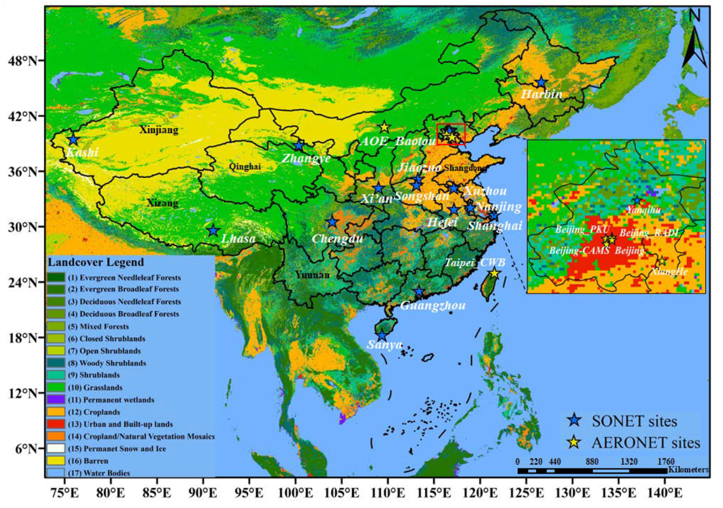
2.1. Study Area

The territory of China was the study area, and its land cover types are shown in Figure 1. According to the MODIS Land Cover Type (MCD12Q1) International Geosphere-Biosphere Programme (IGBP) classification, China has 17 land cover types (as shown in

Table 1. Seventeen land cover types of MCD12Q1 IGBP classification.

Number	Land Cover Type	Number	Land Cover Type
(1)	Evergreen Needleleaf Forests	(10)	Grasslands
(2)	Evergreen Broadleaf Forests	(11)	Permanent Wetlands
(3)	Deciduous Needleleaf Forests	(12)	Croplands
(4)	Deciduous Broadleaf Forests	(13)	Urban and Built-up Lands
(5)	Mixed Forests	(14)	Cropland/Natural Vegetation Mosaics
(6)	Closed Shrublands	(15)	Permanent Snow and Ice
(7)	Open Shrublands	(16)	Barren
(8)	Woody Savannas	(17)	Water Bodies
(9)	Savannas

). The spatial resolution was 500 m [50]. It can be seen that China comprises all surface types, with vast deserts and grasslands distributed in the northwest, croplands mainly located in the east and northeast, forests in the south and northeast, and urban cities mainly distributed in the east and along the coastal area. Furthermore, China is currently the biggest developing country globally and has the largest population; with its rapid development in the past few decades, China has become one of the primary sources of aerosols globally. Thus, satellite aerosol remote sensing over China is necessary and has always been a research hotspot. However, due to the complexity of the aerosol sources and land cover, aerosol retrieval over China is still a great challenge.

2.2. Datasets

2.2.1. DPC Data

The DPC is the first Chinese multiangle polarized satellite sensor. A two-day revisit period enables the DPC to effectively monitor the temporal variation in aerosols, and it crosses the equator at about 13:30 local solar time. A more detailed introduction to the DPC can be found in Li et al. [15]. According to Zhu et al. [51], the calibration uncertainties of the DPC are about 1–7% depending on the wavelength and view zenith angle. This study used thirteen months (March 2019 to March 2020) of DPC multiangle multispectral (443, 490, 670, and 865 nm) intensity data to retrieve AOD using the VISRR algorithm. The DPC data can be downloaded from the High-Resolution Earth Observation System Grid Platform/Chinese National Space Administration Earth Observation and Data Center website (https://www.cheosgrid.org.cn/) (accessed on 17 May 2022).

2.2.2. MODIS Products

MODIS is a multispectral sensor with 36 channels ranging from 0.412 to 14.2 μm onboard the Terra and Aqua satellites, which cross the equator at about 10:30 and 13:30 local solar time each day, respectively. MODIS has observed the earth for more than 20 years and provided many land and atmospheric products from both the Terra (‘MOD’) and Aqua (‘MYD’) satellites. Bands 1–10 (b1–10) are as follows: b1 (620–670 nm), b2 (841–876 nm), b3 (459–479 nm), b4 (545–565 nm), b5 (1230–1250 nm), b6 (1628–1652 nm), b7 (2105–2155 nm), b8 (405–420 nm), b9 (438–448 nm), and b10 (483–493 nm). MODIS products can be downloaded from the website of NASA (https://ladsweb.modaps.eosdis.nasa.gov/) (accessed on 15 August 2022). The MODIS products used here included MYD09; MCD43D; MYD08_D; MCD12Q1; and some aerosol products (MYD04_L2_DT, MYD04_L2_DB, and MYD04_3k_DT). Detailed information on these products is listed in Supplementary Materials Section S1.

2.2.3. Elevation Data

Global Multiresolution Terrain Elevation Data 2010 (GMTED2010) is a global elevation model developed by the U.S. Geological Survey (USGS, https://usgs.gov/) (accessed on 15 August 2022) and National Geospatial Intelligence Agency (NGA), which has three spatial resolutions of about 1 km, 500 m, and 250 m [52]. In this study, GMTED2010 data were used to determine the altitude and correct the influence of Rayleigh scattering for the DPC.

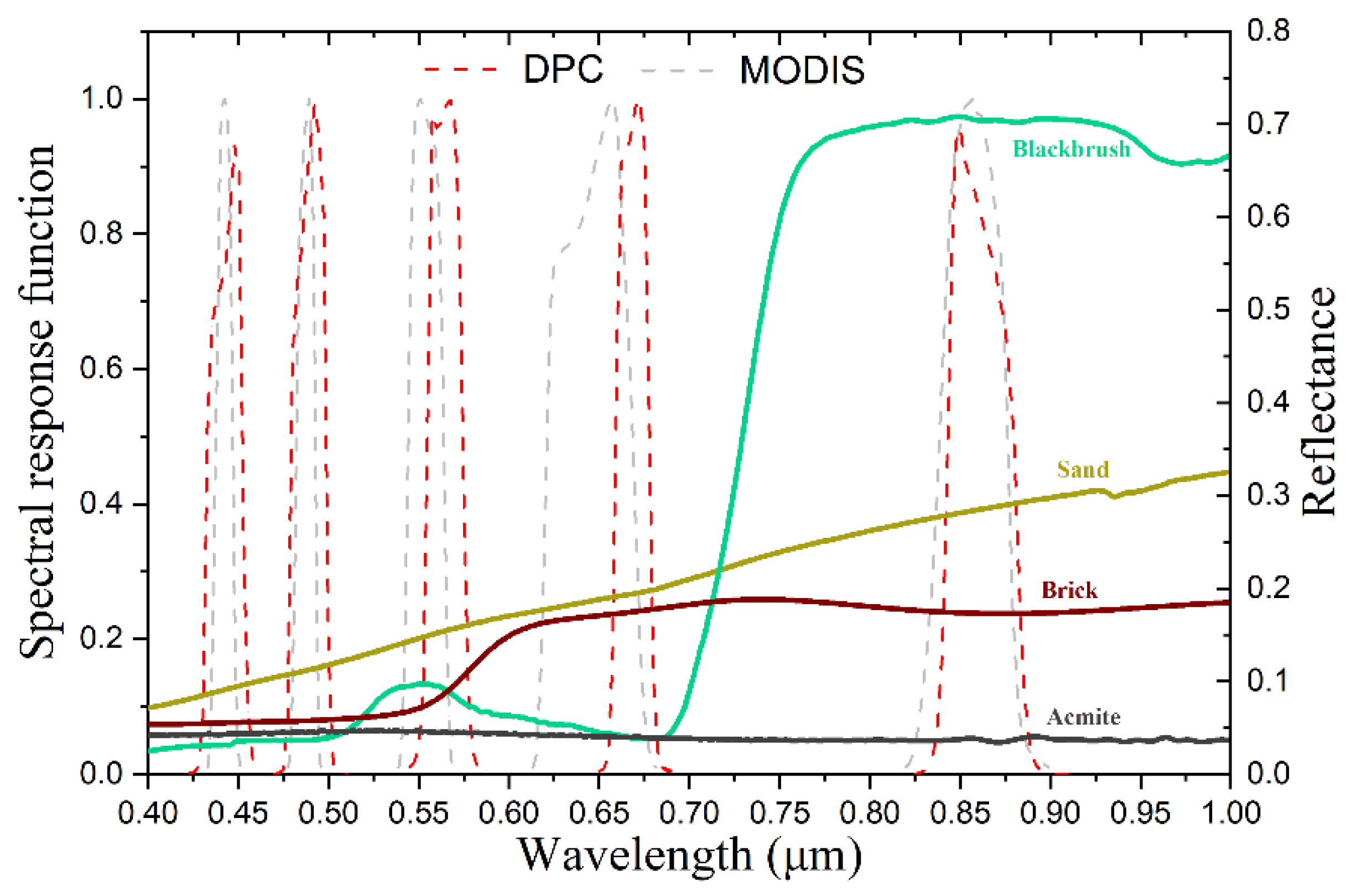
2.2.4. Spectral Library

The USGS spectral library is a reference database containing seven categories of reflectance spectra (artificial materials, coatings, liquids, minerals, organic compounds, soils and mixtures, and vegetation) measured using laboratory, field, and airborne spectrometers [53]. The Spectral Library Version07b (Splib07b) datasets were used to analyze the characteristic variety of the surface spectra between different bands, in order to adjust the spectral response function (SRF) differences between DPC and MODIS for corresponding bands.

2.2.5. Ground-Based Products

Ground-based aerosol products are widely used to validate satellite aerosol remote sensing. AERONET (https://aeronet.gsfc.nasa.gov/) (accessed on 15 August 2022) is a global network established by NASA GSFC (Goddard Space Flight Center) and PHOTONS (PHOtométrie pour le Traitement Opérationnel de Normalisation Satellitaire), according to Giles et al. [1], and the uncertainty of the VIS and NIR AERONET AOD is estimated to be 0.01 for Version 3 (V3) products. However, AERONET sites are rare and distributed unevenly over China. Thus, the Chinese ground-based aerosol observation network SONET (http://www.sonet.ac.cn/en/index.php) (accessed on 15 August 2022) was built by the Chinese Academy of Sciences in collaboration with universities and institutes. The sites of SONET are widely distributed in the typical area of China [2]. In this study, twenty-two AERONET and SONET sites were chosen to validate the DPC and MODIS aerosol products. The spatial distribution and detailed information related to these sites are presented in Figure 1 and

Table 2. Twenty-two ground-based sites of AERONET and SONET and their locations, elevations, surface types, and network.

Number	Site Name	Longitude (°E)	Latitude (°N)	Elevation (m)	Surface Type	Network
1	Hefei	117.162	31.905	36	Cropland	SONET
2	XiangHe	116.962	39.754	36	Cropland	AERONET
3	Zhangye	100.364	38.854	1364	Cropland	SONET
4	AOE_Baotou	109.629	40.852	1314	Grassland	AERONET
5	Lhasa	91.088	29.648	3678	Grassland	SONET
6	Sanya	109.379	18.290	29	Forest	SONET
7	Yanqihu	116.674	40.408	100	Forest	SONET
8	Kashi	75.930	39.504	1320	Mixed	SONET
9	Jiaozuo	113.253	35.187	59	Mixed	SONET
10	Songshan	113.096	34.535	475	Mixed	SONET
11	Beijing	116.381	39.977	92	Urban	AERONET
12	Beijing_PKU	116.310	39.992	53	Urban	AERONET
13	Beijing_RADI	116.379	40.005	59	Urban	AERONET
14	Beijing-CAMS	116.317	39.933	106	Urban	AERONET
15	Chengdu	103.9891	30.5839	510	Urban	SONET
16	Guangzhou	113.381	23.06	28	Urban	SONET
17	Harbin	126.614	45.705	223	Urban	SONET
18	Nanjing	118.957	32.115	52	Urban	SONET
19	Xi’an	109.001	34.223	389	Urban	SONET
20	XuZhou	117.142	34.217	60	Urban	SONET
21	Shanghai	121.481	31.284	84	Urban	SONET
22	Taipei_CWB	121.538	25.015	26	Urban	AERONET

. In addition, these sites were divided into five surface types according to MCD12Q1 [54].

3. Basic Principles and New Methodology

3.1. Surface BRDF Model

This study adopted a linear semi-empirical kernel-driven RossThick LiSparseReciprocal (RTLSR) BRDF model to describe the anisotropic SR [55,56]. The RTLSR model has been widely used in many types of research and has obtained good results [57,58]. Meanwhile, the RTLSR model was adopted to produce MODIS and VIIRS global operational BRDF products [59,60]. The equation of the RTLSR model is as follows:

$$\begin{gathered} R_{SR}\left(\lambda ,{\theta }_s,{\theta }_v,\varnothing \right)=f_{iso}\left(\lambda \right) K_{iso}\left({\theta }_s,{\theta }_v,\varnothing \right)+f_{vol}\left(\lambda \right) K_{vol}\left({\theta }_s,{\theta }_v,\varnothing \right) \\ +f_{geo}\left(\lambda \right) K_{geo}\left({\theta }_s,{\theta }_v,\varnothing \right) \end{gathered}$$

(1)

where $\lambda$ is the wavelength; ${\theta }_s,{\theta }_v,\mathrm{and} \varnothing$ are solar zenith angle, sensor zenith angle, and relative azimuth angle, respectively; $R_{SR}$ represents the surface directional reflectance; $K_{iso}$, $K_{vol}$, and $K_{geo}$ represent the isotropic, volumetric, and geometric kernels, respectively, where $K_{iso}=1$, and the expression of $K_{vol}$ and $K_{geo}$, which are fixed functions and only dependent on the solar and viewing geometry, can be found in Wanner et al. [61]; and $f_{iso}\left(\lambda \right)$, $f_{geo}\left(\lambda \right),$ and $f_{vol}\left(\lambda \right)$ are the coefficients of the three kernels, which were varied according to the wavelength and surface characteristics. Furthermore, Equation (1) could be separated into two terms:

$$R_{SR}\left(\lambda ,{\theta }_s,{\theta }_v,\varnothing \right)=\rho \left(\lambda \right)\left[1+{\alpha }_1\left(\lambda \right) K_{vol}\left({\theta }_s,{\theta }_v,\varnothing \right)+{\alpha }_2\left(\lambda \right) K_{geo}\left({\theta }_s,{\theta }_v,\varnothing \right)\right]$$

(2)

where $\rho \left(\lambda \right)=f_{iso}\left(\lambda \right)$ indicates the “reflectance magnitude”, which is governed by surface type microphysical properties and changes rapidly with wavelength and time; ${\alpha }_1$ and ${\alpha }_2$ represent the geometric factor and volumetric factor, respectively; ${\alpha }_1\left(\lambda \right)=\frac{f_{vol}\left(\lambda \right)}{f_{iso}\left(\lambda \right)}$; and ${\alpha }_2\left(\lambda \right)=\frac{f_{geo}\left(\lambda \right)}{f_{iso}\left(\lambda \right)}$. The part in the square bracket is the BRDF shape ($BRD{F}_s$) function (Equation (3)), which is based on the macroscopic structure of the surface types, remains nearly independent of the wavelength, and changes slowly in a short time [62]:

$$BRD{F}_s=1+{\alpha }_1\left(\lambda \right) K_{vol}\left({\theta }_s,{\theta }_v,\varnothing \right)+{\alpha }_2\left(\lambda \right) K_{geo}\left({\theta }_s,{\theta }_v,\varnothing \right)$$

(3)

3.2. Atmospheric Radiative Transfer Model

Overlying the Lambertian homogeneous surface and under cloud-free, plane-parallel atmosphere conditions, the satellite sensor received reflectance ($R_{TOA}$) at the top of atmosphere (TOA) can be written as:

$$R_{TOA}\left(\lambda ,\tau ,{\theta }_s,{\theta }_v,\varnothing \right)=T_g\left(R_{atm}\left(\lambda ,\tau ,{\theta }_s,{\theta }_v,\varnothing \right)+\frac{T^{\downarrow }\left({\theta }_s\right)R_{SR}{T}^{\uparrow }\left({\theta }_v\right)}{1-R_{SR}S}\right)$$

(4)

where $\tau$ is the optical depth; $T_g$ indicates the gaseous transmission caused by gases such as column water vapor (CWV) and ozone (O₃); $R_{atm}$ refers to the aerosol and molecular intrinsic reflectance; $T^{\downarrow }$ and $T^{\uparrow }$ are transmission; $S$ is the spherical albedo of the atmosphere; and $R_{SR}$ is the angular SR.

SR is an anisotropic Lambertian surface hypothesis can affect the accuracy of the $R_{TOA}$ simulation, especially for multiangle data, ultimately transferring the error to the aerosol retrieval [63]. To avoid this problem in the present study, a fast, accurate, non-Lambertian atmospheric radiative transfer function considering the anisotropy of the surface based on the four-stream theory was adopted. This function has high precision, with mean relative differences in the spectral (range from UV to NIR) TOA simulation of less than 0.7% for different surface types [64]. This forward model has been widely used for aerosol and surface parameter retrieval [65,66,67], and the equation can be expressed as:

$$R_{TOA}\left(\lambda ,\tau ,{\theta }_s,{\theta }_v,\varnothing \right)=T_g(R_{atm}\left(\lambda ,\tau ,{\theta }_s,{\theta }_v,\varnothing \right)+\frac{\overrightarrow{T}{\left({\theta }_s\right)}^T \mathit{R} \overrightarrow{T}\left({\theta }_v\right)-e^{-\tau /{\theta }_s}\left|\mathit{R}\right|e^{-\tau /{\theta }_v}S}{1-R_{BHR}S})$$

(5)

where $\overrightarrow{T}\left({\theta }_s\right)={\left[e^{-\tau /{\theta }_s}, t_s\left({\theta }_s\right)\right]}^T$; $\overrightarrow{T}\left({\theta }_v\right)={\left[e^{-\tau /{\theta }_v}, t_s\left({\theta }_v\right)\right]}^T$; $t_s\left({\theta }_{s/v}\right)$ refers to the diffuse transmission; $\mathit{R}$ is the reflectance matrix; and $\left|\mathit{R}\right|$ is the determinant of $\mathit{R}$.

$$\mathit{R}=\left[\begin{array}{cc}{R}_{SR}& R_{DHR}\\ R_{HDR}& R_{BHR}\end{array}\right]$$

(6)

$$\left|\mathit{R}\right|=\left(R_{SR}{R}_{BHR}-R_{DHR}{R}_{HDR}\right)$$

(7)

where $R_{DHR}$ represents the directional–hemispherical reflectance (DHR), i.e., black-sky albedo ($R_{bs}$), which describes the diffuse reflection of the incoming direct beam over the hemisphere; $R_{HDR}$ refers to the hemispherical–directional reflectance (HDR), which describes the direct reflection of the incoming diffuse radiation from the whole hemisphere; and $R_{BHR}$ is the bi-hemispherical reflectance (BHR), i.e., white-sky albedo.

When the coefficients of the three kernels are obtained, the SR for any angle can be calculated with Equation (1). Meanwhile, the $R_{DHR}$ and $R_{BHR}$ can be computed using the following Equations (8)–(11) [67]:

$$R_{DHR}\left(\lambda ,{\theta }_s\right)=f_{iso}\left(\lambda \right)h_{iso}\left({\theta }_s\right)+f_{vol}\left(\lambda \right)h_{vol}\left({\theta }_s\right)+f_{geo}\left(\lambda \right)h_{geo}\left({\theta }_s\right)$$

(8)

$$R_{HDR}\left(\lambda ,{\theta }_v\right)=f_{iso}\left(\lambda \right)h_{iso}\left({\theta }_v\right)+f_{vol}\left(\lambda \right)h_{vol}\left({\theta }_v\right)+f_{geo}\left(\lambda \right)h_{geo}\left({\theta }_v\right)$$

(9)

$$R_{BHR}\left(\lambda \right)=f_{iso}\left(\lambda \right)H_{iso}+f_{vol}\left(\lambda \right)H_{vol}+f_{geo}\left(\lambda \right)H_{geo}$$

(10)

$$h_k\left({\theta }_s\right)=g_{0k}+g_{1k}{\theta }_s+g_{2k}{\theta }_s{}^2+g_{3k}{\theta }_s{}^3$$

(11)

where $H_k$ and $g_{ik}$ ($i$ = 0, 1, 2, 3; $k$ = iso, vol, geo) are the regression coefficients listed in

Table 3. Regression coefficients used to calculate black-sky and white-sky albedo.

$\mathbf{Term} {\mathit{g}}_{\mathit{i}\mathit{k}}$ for Kernel	$\mathit{k}$ = iso	$\mathit{k}$ = vol	$\mathit{k}$ = geo
$g_{0k}$	1.0	−0.0374	−1.2665
$g_{1k}$	0.0	0.5699	−0.1662
$g_{2k}$	0.0	−1.1252	0.1829
$g_{3k}$	0.0	0.8432	−0.1489
White-sky integral ($H_k$)	1.0	0.189184	−1.377622

.

3.3. VISRR Algorithm

VISRR is a novel AOD retrieval algorithm, which uses the SRRs between VIS bands as constraints and considers the influence of surface anisotropy. VISRR can simultaneously retrieve AOD over dark and bright land covers; the algorithm derivation and retrieval strategies are described in detail below.

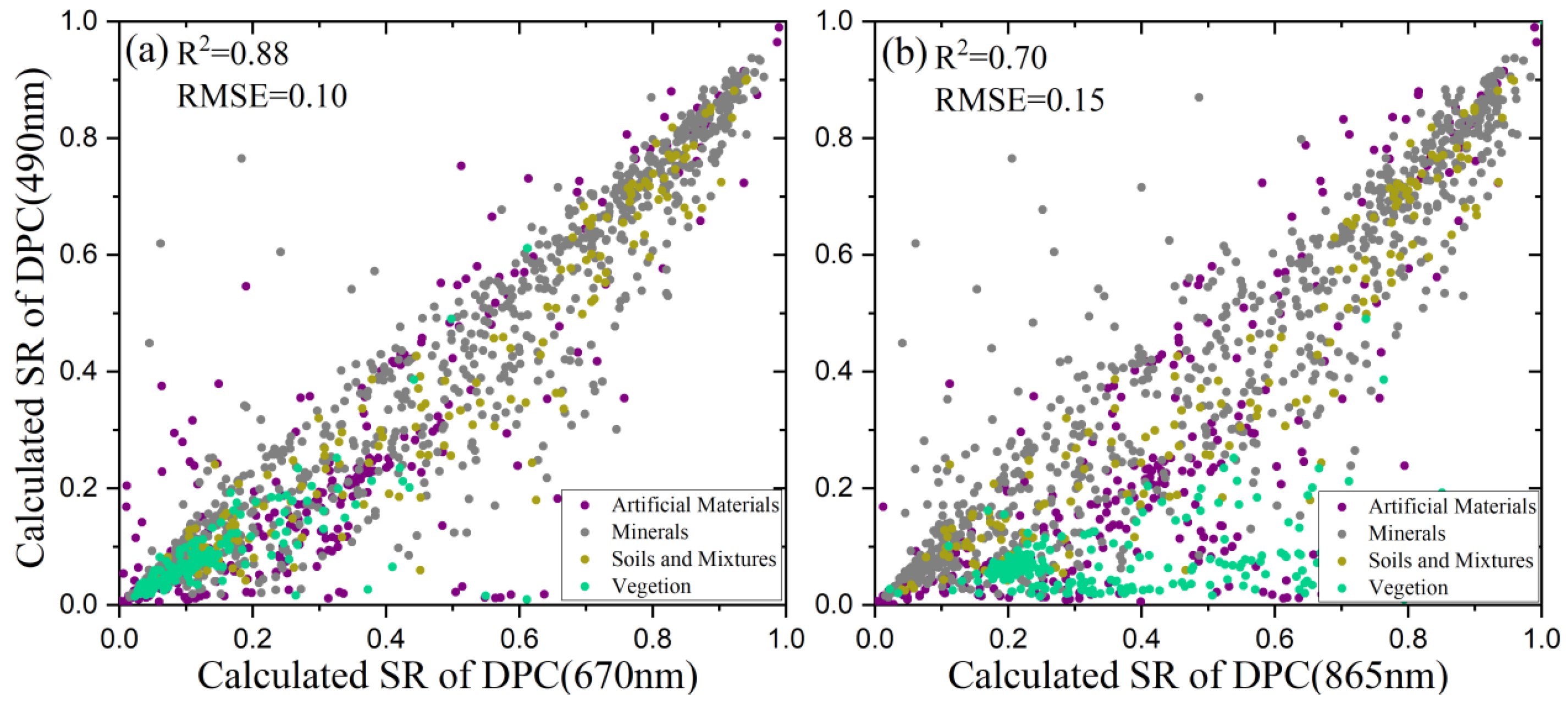
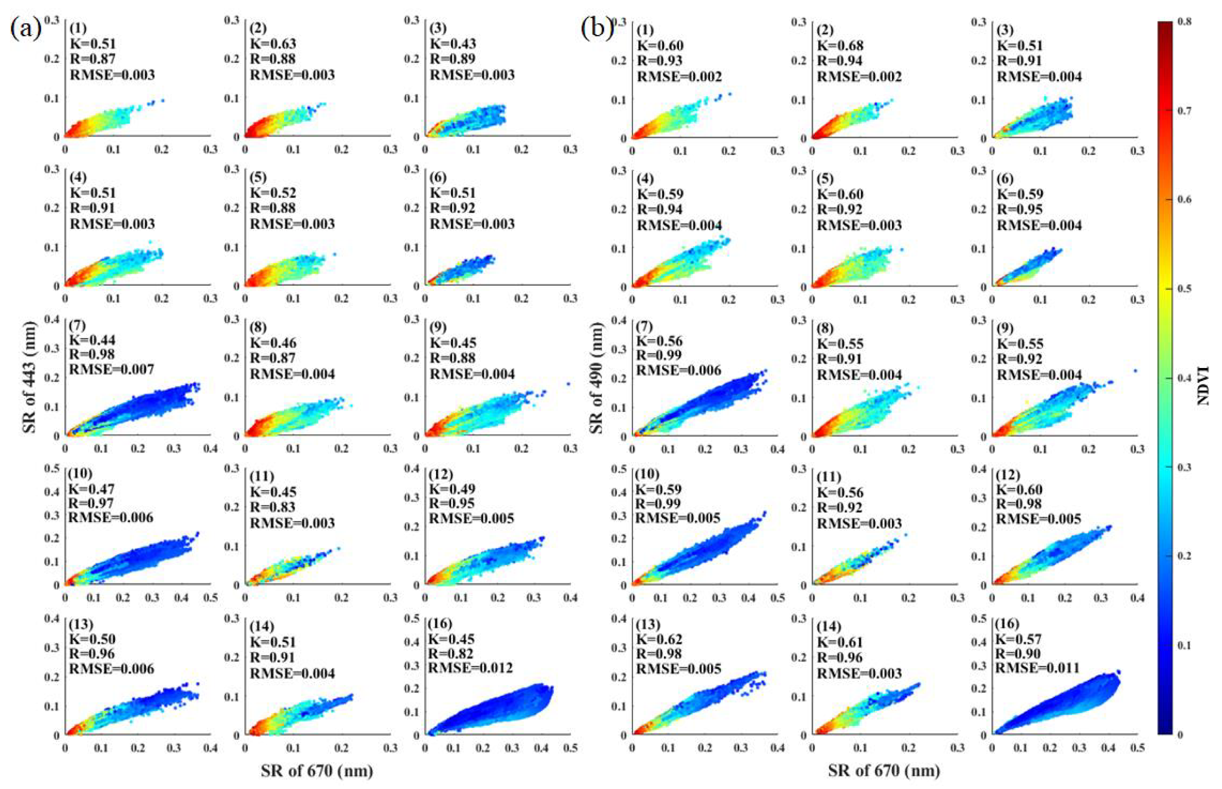
3.3.1. SR Characteristics Analysis

Firstly, we used the Splib07b spectral library to analyze which bands were suitable for aerosol retrieval. Figure 2 shows the SRFs of the DPC in the 443, 490, 565, 670, and 865 nm bands (red dotted line) and the corresponding MODIS b9, b10, b5, b1, and b2 bands (gray dotted line). Curves of different colors represent the SR spectral curves of typical surface materials (i.e., blackbrush, sand, brick, and acmite) from Splib07b. From the picture, it can be seen that the surface contribution of VIS is much lower than that of NIR; the SR of non-green vegetation (i.e., sand and brick) is higher than that of green vegetation (i.e., blackbrush); and for green vegetation, there exist two high-reflection peaks near 565 and 865 nm. These features mean that VIS bands are more suitable for aerosol retrieval than NIR bands; aerosol retrieval over green vegetation is easier than over non-green vegetation; and the green band (565 nm) may not be suitable for aerosol retrieval over green vegetation cover. Furthermore, we analyzed the SRRs between the VIS and NIR bands; Figure 3a,b show the SRRs between 490 and 670 nm and between 490 and 865 nm, respectively. It can be seen that the SRRs between VIS bands are more stable than those between VIS and NIR bands, which is consistent with Levy’s research [19]. This phenomenon can be explained by the fact that most ground objects have similar spectral reflectance changes in the VIS spectrum range but large changes in the NIR or SWIR bands. Thus, the 443, 490, and 670 nm bands were chosen to build the SRRs in this study.

3.3.2. SR Relationship Analysis

Within a satellite sensor’s instantaneous field of view, individual pixels detected by the scanning device often include more than one object, especially those with a spatial resolution at the kilometer level. Thus, the determination of SRRs requires real satellite data. Two common methods are used to construct the target sensor’s prior knowledge of spectral SR for aerosol retrieval. One is to apply a minimum reflectivity technique [17,68] or atmospheric correction to the target sensor’s data [7,19]. This method is suitable for target sensors with long-time-series data that can provide enough samples. The other method is to use the mature SR products from other satellite sensors, such as MODIS [69,70]. This method is generally applicable to new sensors. In this study, owing to the limitation of the relatively small amount of DPC data, the second method was chosen, and three years (2016–2018) of MYD09 SR products pertaining to China and its surrounding areas (Figure 1) were used to derive the DPC equivalent spectrum SR over different surface types. To ensure the accuracy of the SR, only the pixels with an AOD at 470 nm smaller than 0.2 and the highest quality assurance (QA) of MYD09 were chosen for analysis.

However, two problems needed to be solved beforehand, since DPC and MODIS differ in terms of spatial resolution (3.3 versus 1 km) and SRFs (as shown in Figure 2). To make the spatial resolution consistent, about 3 $\times$ 3 pixels of MYD09 and MYD03 were averaged at 3.3 km. As shown in Figure 2, the SRFs of DPC and MODIS do not exactly match; if we did not consider these differences, it would have led to errors in the derived equivalent spectral SR of DPC and affected the accuracy of the aerosol retrieval [70]. We adopted the singular-value decomposition (SVD) method to predict the DPC equivalent spectral SR from the corresponding MODIS channels to solve this problem. The steps were as follows: (1) we used the SRFs and the spectral curves of typical surface materials from Splib07b to calculate the DPC and MODIS spectral SR; (2) we calculated the SVDs, which included the singular vectors $V_{modis}$ and $V_{DPC}$, based on the calculated spectral SR from step (1); (3) we used the $V_{modis}$ and MYD09 SR products to calculate the conversion coefficient vector $C$; and (4) the DPC equivalent spectrum SR could be calculated using the $C$ and the $V_{DPC}$. Detailed information on this method can be found in Sayer et al. [70].

After obtaining the equivalent spectrum SR and geometric information on the DPC over different surface types (except for permanent snow, ice, and water), we analyzed the SRRs between 443, 490, and 670 nm. The normalized difference vegetation index (NDVI) is an important adjustment parameter to estimate the SR for aerosol retrieval [19,20,71], and it can be calculated by the SR of 670 and 865 nm using Equation (12):

$$NDVI=\frac{SR\left(865\right)-SR\left(670\right)}{SR\left(865\right)+SR\left(670\right)}$$

(12)

The statistical results of the SRRs are shown in Figure 4. It can be seen that the Pearson correlation coefficient (R) of 443 versus 670 nm ranged from 0.82 to 0.98, the root mean square error (RMSE) ranged from 0.003 to 0.012, and the average SR ratios ($K_{443\_670}$) over different surface types varied from 0.43 to 0.63. For 490 and 670 nm, the R ranged from 0.90 to 0.99, the RMSE ranged from 0.002 to 0.011, and the $K_{490\_670}$ over different surface types varied from 0.51 to 0.68. These statistical parameters showed that: (1) the SRRs between VIS bands had a high correlation, which was consistent with the conclusion of Section 3.3.1; (2) the SRRs between VIS bands needed to be divided according to the surface types due the substantial differences; (3) the correlation of SRRs between 490 and 670 nm was higher than that between 443 and 670 nm overall; and (4) the NDVI could indicate the surface type and the change in the SR over time to a certain extent—for example, the NDVI of evergreen vegetation (e.g., Figure 4(1,2)) usually has a high value, while over bare soil (e.g., Figure 4(16)) it has a low value. When the surface types vary significantly with the seasons, the NDVI also has a wider range of changes (e.g., Figure 4(10,13)). It is necessary to consider surface types and NDVI when using the SRRs between VIS bands as constraints for aerosol retrieval.

In addition, to make the SRRs between VIS bands more accurate, the SCA was also taken into account when determining the $K_{443\_670}$ and $K_{490\_670}$ over different surface types. The final values of $K_{443\_670}$ and $K_{490\_670}$ over each typical surface type are shown in

Table 4. Variation in $K_{443\_670}$ and $K_{490\_670}$ with NDVI and SCA over (5) mixed forests.

NDVI/SCA	(60°, 100°)		(100°, 120°)		(120°, 140°)		(140°, 160°)		(160°, 180°)
	${\mathit{K}}_{443\_670}$	${\mathit{K}}_{490\_670}$	${\mathit{K}}_{443\_670}$	${\mathit{K}}_{490\_670}$	${\mathit{K}}_{443\_670}$	${\mathit{K}}_{490\_670}$	${\mathit{K}}_{443\_670}$	${\mathit{K}}_{490\_670}$	${\mathit{K}}_{443\_670}$	${\mathit{K}}_{490\_670}$
(0.0, 0.2)	0.51	0.68	0.49	0.60	0.47	0.57	0.49	0.58	0.56	0.60
(0.2, 0.4)	0.49	0.61	0.50	0.61	0.48	0.56	0.51	0.59	0.56	0.62
(0.4, 0.6)	0.49	0.64	0.50	0.63	0.47	0.57	0.52	0.61	0.59	0.65
(0.6, 0.8)	0.53	0.64	0.51	0.63	0.51	0.62	0.53	0.61	0.59	0.64
(0.8, 1.0)	0.51	0.62	0.51	0.62	0.58	0.66	0.62	0.65	0.62	0.62

,

Table 5. Same as Table 4, but for (10) grasslands.

NDVI/SCA	(60°, 100°)		(100°, 120°)		(120°, 140°)		(140°, 160°)		(160°, 180°)
	${\mathit{K}}_{443\_670}$	${\mathit{K}}_{490\_670}$	${\mathit{K}}_{443\_670}$	${\mathit{K}}_{490\_670}$	${\mathit{K}}_{443\_670}$	${\mathit{K}}_{490\_670}$	${\mathit{K}}_{443\_670}$	${\mathit{K}}_{490\_670}$	${\mathit{K}}_{443\_670}$	${\mathit{K}}_{490\_670}$
(0.0, 0.2)	0.49	0.68	0.43	0.53	0.43	0.54	0.48	0.56	0.49	0.52
(0.2, 0.4)	0.53	0.65	0.44	0.56	0.45	0.55	0.46	0.55	0.44	0.50
(0.4, 0.6)	0.51	0.65	0.42	0.55	0.44	0.56	0.47	0.57	0.48	0.54
(0.6, 0.8)	0.53	0.64	0.48	0.62	0.48	0.60	0.48	0.57	0.49	0.55
(0.8, 1.0)	0.53	0.64	0.53	0.64	0.56	0.64	0.59	0.65	0.56	0.61

,

Table 6. Same as Table 4, but for (12) croplands.

NDVI/SCA	(60°, 100°)		(100°, 120°)		(120°, 140°)		(140°, 160°)		(160°, 180°)
	${\mathit{K}}_{443\_670}$	${\mathit{K}}_{490\_670}$	${\mathit{K}}_{443\_670}$	${\mathit{K}}_{490\_670}$	${\mathit{K}}_{443\_670}$	${\mathit{K}}_{490\_670}$	${\mathit{K}}_{443\_670}$	${\mathit{K}}_{490\_670}$	${\mathit{K}}_{443\_670}$	${\mathit{K}}_{490\_670}$
(0.0, 0.2)	0.47	0.61	0.50	0.64	0.45	0.57	0.44	0.54	0.52	0.61
(0.2, 0.4)	0.49	0.62	0.52	0.64	0.52	0.65	0.45	0.56	0.43	0.52
(0.4, 0.6)	0.46	0.60	0.50	0.66	0.46	0.63	0.46	0.57	0.46	0.55
(0.6, 0.8)	0.53	0.67	0.51	0.65	0.50	0.65	0.47	0.57	0.47	0.56
(0.8, 1.0)	0.57	0.65	0.57	0.65	0.57	0.65	0.63	0.68	0.63	0.68

,

Table 7. Same as Table 4, but for (13) urban and built-up lands.

NDVI/SCA	(60°, 100°)		(100°, 120°)		(120°, 140°)		(140°, 160°)		(160°, 180°)
	${\mathit{K}}_{443\_670}$	${\mathit{K}}_{490\_670}$	${\mathit{K}}_{443\_670}$	${\mathit{K}}_{490\_670}$	${\mathit{K}}_{443\_670}$	${\mathit{K}}_{490\_670}$	${\mathit{K}}_{443\_670}$	${\mathit{K}}_{490\_670}$	${\mathit{K}}_{443\_670}$	${\mathit{K}}_{490\_670}$
(0.0, 0.2)	0.49	0.62	0.47	0.60	0.49	0.60	0.52	0.60	0.56	0.63
(0.2, 0.4)	0.48	0.60	0.47	0.60	0.49	0.60	0.52	0.60	0.55	0.61
(0.4, 0.6)	0.50	0.64	0.48	0.63	0.49	0.62	0.52	0.62	0.53	0.61
(0.6, 0.8)	0.48	0.61	0.48	0.62	0.50	0.63	0.52	0.63	0.54	0.62
(0.8, 1.0)	0.49	0.62	0.49	0.64	0.52	0.64	0.53	0.62	0.54	0.63

and

Table 8. Same as Table 4, but for (16) barren land.

NDVI/SCA	(60°, 100°)		(100°, 120°)		(120°, 140°)		(140°, 160°)		(160°, 180°)
	${\mathit{K}}_{443\_670}$	${\mathit{K}}_{490\_670}$	${\mathit{K}}_{443\_670}$	${\mathit{K}}_{490\_670}$	${\mathit{K}}_{443\_670}$	${\mathit{K}}_{490\_670}$	${\mathit{K}}_{443\_670}$	${\mathit{K}}_{490\_670}$	${\mathit{K}}_{443\_670}$	${\mathit{K}}_{490\_670}$
(0.0, 0.2)	0.45	0.70	0.49	0.63	0.49	0.62	0.52	0.60	0.50	0.54
(0.2, 0.4)	0.52	0.64	0.50	0.63	0.51	0.63	0.52	0.61	0.50	0.55
(0.4, 0.6)	0.51	0.60	0.51	0.66	0.51	0.63	0.53	0.62	0.51	0.58
(0.6, 0.8)	0.46	0.56	0.50	0.64	0.54	0.64	0.54	0.63	0.52	0.58
(0.8, 1.0)	0.57	0.64	0.57	0.64	0.60	0.68	0.61	0.67	0.52	0.57

(mixed forests, grasslands, croplands, urban and built-up lands, and barren land). The NDVI was set from 0 to 1 with an interval of 0.2; the SCA was set from 60° to 100° and from 100° to 180° with an interval of 20°. The ratios over other surface types (i.e., (1)–(4), (6)–(9), (14), and (18)–(21)) are shown in Supplemental Materials Section S2, Tables S1–S10.

$$\Theta =co{s}^{-1}\left(-cos{\theta }_{s}cos{\theta }_v-sin{\theta }_{s}sin{\theta }_{v}cos\varnothing \right)$$

(13)

3.3.3. Aerosol Models

The aerosol model is another essential prior knowledge component, and its accuracy plays a vital role in the satellite remote sensing of aerosols [72]. Several global and regional aerosol models derived from AERONET measurements [35,36,37] have been used for many research satellite aerosol retrieval methods. However, these models may not be very representative in China, where ground-based sites are sparse and distributed unevenly. For example, the aerosol models used in the VIIRS enterprising processing system (EPS) aerosol retrieval algorithm have been validated as unsatisfactory in China [44]. Thus, based on the long-time-series data of the SONET, Li et al. [40] used the K-means cluster analysis approach and obtained ten fundamental aerosol models for China, including five typical fine-particle aerosol models ((1) urban polluted, (2) secondary polluted, (3) combined polluted, (4) polluted fly ash, and (5) continental background) and five coarse models ((6) summer fly ash, (7) winter fly ash, (8) primary dust, (9) transported dust, and (10) background dust). Li et al. [40] also provided the probability of the appearance of fine-mode aerosols and coarse-mode aerosols. In this study, we adopted the six combinations with the highest probability of appearance for aerosol retrieval, i.e., urban polluted and summer fly ash, secondary polluted and summer fly ash, combined polluted and winter fly ash, continental background and background dust, continental background and winter fly ash, and continental background and transported dust. The microphysical parameters of these aerosol models can be found in Li et al. [40].

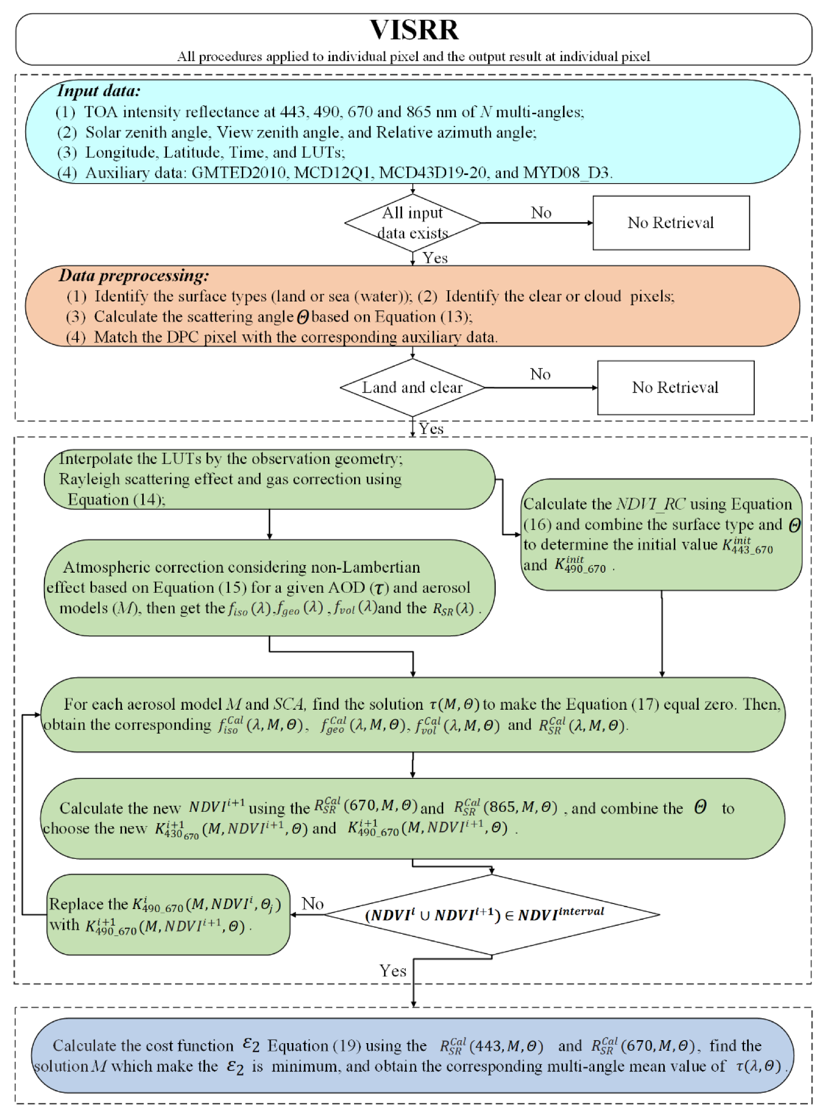
3.3.4. Retrieval Scheme

In this study, the VISRR algorithm was implemented based on the precalculated LUTs, which were built by the second simulation of a satellite signal in the solar spectrum vector (6SV) radiative transfer (RT) model [73]. The input parameters of the 6SV RT model included the SRFs of DPC 443, 490, 670, and 865 nm; six combinations of fine-mode aerosols and coarse-mode aerosols, as shown in Section 3.3.3; ${\theta }_s$ and ${\theta }_v$ ranging from 0$°$ to 80$°$ with an interval of 6$°$; $\varnothing$ ranging from 0$°$ to 180$°$ with an interval of 12$°$; 11 AOD values (550 nm)—0, 0.01, 0.25, 0.5, 1, 1.5, 2, 2.5, 3, 4, 5; and elevation set to sea level. Then, atmospheric parameters (i.e., $R_{atm}$, $\overrightarrow{T}\left({\theta }_s\right)$, $\overrightarrow{T}\left({\theta }_v\right)$, $t_s\left({\theta }_s\right)$, and $t_s\left({\theta }_v\right)$ in Equation (4)) for various observational and atmospheric scenarios were built in the LUTs. Similarly, the LUTs of CWV and O₃ gas transmission were also built by the 6SV RT model. The value of CWV was set in the range of 0 to 7 g/cm² with an interval of 0.5, and the value of O₃ was set in the range of 0 to 5 cm-atm with an interval of 0.5. In this study, the prior knowledge of BRDF shape (Equation (3)) was assumed to be unchanged for one month and independent of bands [62,65]. When the LUTs and related auxiliary data were ready, the VISRR algorithm could be performed based on the multiangle multispectral DPC intensity data. All procedures were applied to the individual pixels, and the output result at each pixel was recorded. The schematic flowchart is shown in Figure 5, and the specific retrieval steps are described below.

(a)

Preprocessing the input data

The input parameters of the DPC included the measured TOA reflectance ($R_{TOA}^{Meas}\left(\lambda \right)$) of 443, 490, 670, and 865 nm, with N (maximum of 12) multiangle (${\theta }_s,{\theta }_v,\varnothing$), and the auxiliary datasets included month-averaged MCD43D19-21, MYD08_D3, GMTED2010, MCD12Q1, and the LUTs.

The first step was the identification of the land surface type for each pixel using the MCD12Q1 products; second was the recognition of cloud-contaminated pixels, as only cloud-free and land (except for permanent snow, ice, or inland water) pixels were further processed in the next step; and third was to match and extract the auxiliary data according to the longitude, latitude, the corresponding geometric factor ${\alpha }_1$ and volumetric factor ${\alpha }_2$ of the BRDF shape, the daily O₃ and CWV, and the elevation from the month-averaged MCD43D19-20, MYD08_D3, and GMTED2010 products. The global mean values were adopted if the O₃ and CWV were missing from MYD08_D3, as shown in Levy et al. [74].

(b)

Atmospheric correction method considering the non-Lambertian effect

(1) According to the observation angle (${\theta }_s,{\theta }_v,\varnothing$), the atmospheric parameters $R_{atm}\left(\lambda ,\tau ,{\theta }_s,{\theta }_v,\varnothing \right)$, $\overrightarrow{T}\left(\lambda ,{\theta }_s\right)$, $\overrightarrow{T}\left(\lambda ,{\theta }_v\right)$, and $S$ varied with $\tau$ and aerosol model (M), and the gas transmission $T_g\left(\lambda \right)$ varied with CWV and O_3, as could be interpolated from the LUTs.

(2) We utilized the Rayleigh scattering correction method proposed by Fraser et al. [75] to remove its contribution to the reflectance at TOA [19] and then obtained the gas corrected reflectance ($R_{TOA}^{Meas\_gasc}\left(\lambda \right)$).

$$R_{TOA}^{Meas\_gasc}\left(\lambda \right)=R_{TOA}^{Meas}\left(\lambda \right)/T_g\left(\lambda \right)$$

(14)

(3) Considering the non-Lambertian characteristics of the surface, the atmospheric correction (AC) was implemented to calculate accurate directional surface reflectance $R_{SR}$($\lambda$). The AC equation is Equation (15), and the detailed derivation process is shown in Supplementary Section S3.

$$F_1 =\frac{f_{iso}\left(\lambda \right)\left(F_2^{\prime }-F_3^{\prime }\right)}{1-f_{iso}\left(\lambda \right)F_4^{\prime }}$$

(15)

where the definitions of $F_1$, $F_2^{\prime }$, $F_3^{\prime }$, $F_4^{\prime }$ can be found in Supplementary Section S3. Then, the three kernel coefficients $f_{iso}\left(\lambda \right)$, $f_{geo}\left(\lambda \right)$, and $f_{vol}\left(\lambda \right)$ of the RTLSR BRDF model and the directional surface reflectance $R_{SR}\left(\lambda \right)$ could be obtained as follows: $f_{iso}\left(\lambda \right)=F_1/(F_2^{\prime }$+$F_3^{\prime }$ + $F_4^{\prime }*F_1)$, $f_{vol}\left(\lambda \right)=f_{iso}\left(\lambda \right){\alpha }_1$, $f_{geo}\left(\lambda \right)=f_{iso}\left(\lambda \right){\alpha }_2$, $f_{geo}\left(\lambda \right)=f_{iso}\left(\lambda \right){\alpha }_2$, $R_{SR}\left(\lambda \right)=f_{iso}\left(\lambda \right)BRD{F}_s$.

(c)

Determination of the initial NDVI value and prior knowledge of $K_{443\_670}$ and $K_{490\_670}$

The NDVI is an important adjustable parameter for estimating SR and has been widely used for aerosol retrieval. However, the NDVI usually cannot be obtained before aerosol retrieval due to the effects of the atmosphere. Thus, some researchers directly use the reflectance at TOA to calculate the NDVI (NDVI_TOA) [76,77] or use the Rayleigh corrected reflectance at TOA to calculate the NDVI (NDVI_RC) to reduce the impact of the atmosphere [20,78]. However, NDVI_TOA and NDVI_RC are still susceptible to aerosols and rapidly decrease with increasing AOD [79,80,81]. The use of NDVI_TOA or NDVI_RC can lead to the selection of the wrong $K_{443\_670}$ and $K_{490\_670}$ values (as shown in Table 3, Table 4, Table 5, Table 6 and Table 7) under some atmospheric conditions and can cause further errors in aerosol retrieval. Thus, to solve this problem, we developed a novel iterative AC method to calculate the real NDVI. Firstly, we used the Rayleigh scattering and gas correction NDVI_RC, which was calculated via Equation (16), as the initial NDVI value (recorded as $NDV{I}^{init}$); then, after combining the SCA and surface type, the initial $K_{443\_670}^{init}$ and $K_{490\_670}^{init}$ could be determined as:

$$\mathrm{NDVI}\_\mathrm{RC}= \frac{R_{TOA}^{Meas\_gasc}\left(865\right)-R_{TOA}^{Meas\_gasc}\left(670\right)}{ R_{TOA}^{Meas\_gasc}\left(865\right)+R_{TOA}^{Meas\_gasc}\left(670\right)}$$

(16)

(d)

AOD retrieval

There were three problems to be solved in this step. The first was the determination of the solution $\tau$ for each aerosol model, the second was the determination of the NDVI, and the third was the determination of the best aerosol model. The steps are described in detail as follows:

(1) For each aerosol model M and $\Theta$, we found the solution $\tau \left(M,\Theta \right)$ that made the cost function ${\epsilon }_1$ (Equation (17)) equal to 0 (i.e., ${\epsilon }_1=0$). Then, we obtained the $R_{SR}^{Cal}\left(\lambda ,M,\Theta \right)$ of 443, 490, 670, and 865 nm:

$${\epsilon }_1\left(M,\Theta \right)=\frac{R_{SR}^{Cal}\left(490,M,{\Theta }_j,\tau \right)}{R_{SR}^{Cal}\left(670,M,{\Theta }_j,\tau \right)}-K_{490\_670}^i\left(M,NDV{I}^i,{\Theta }_j\right)$$

(17)

where $R_{SR}^{Cal}\left(\lambda ,M,\Theta ,\tau \right)$ is the directional surface reflectance calculated using the AC method considering the non-Lambertian effect, as shown in step (c); the superscript i of $NDV{I}^i$ and $K_{490\_670}^i$ represents the number of iterations; and the $NDV{I}^{init}$ and $K_{490\_670}^{init}$ determined in step (d) are the initial values of the iteration (i.e., i = 0).

(2) We calculated the new $NDV{I}^{i+1}$ using the $R_{SR}^{Cal}\left(670,M,\Theta \right)$ and $R_{SR}^{Cal}\left(865,M,\Theta \right)$ obtained from step (1) and determined the new $K_{{430}_{670}}^{i+1}\left(M,NDV{I}^{i+1},\Theta \right)$ and $K_{490\_670}^{i+1}\left(M,NDV{I}^{i+1},\Theta \right)$ values using the $NDV{I}^{i+1}$ and $\Theta$. Then, we considered Formula (18); if the $NDV{I}^i$ and $NDV{I}^{i+1}$ belonged to the same NDVI interval ($NDV{I}^{interval}$) defined in Section 3.3.2, we proceeded to step (3). Otherwise, we repeated (1) and (2) until Formula (18) was satisfied.

$$(NDV{I}^i{{\displaystyle \cup }}^{ }NDV{I}^{i+1})\in NDV{I}^{interval}$$

(18)

(3) We calculated the cost function ${\epsilon }_2$ (Equation (19)) using $R_{SR}^{Cal}\left(443,M,\Theta \right)$, $R_{SR}^{Cal}\left(670,M,\Theta \right),$ and $K_{{430}_{670}}^{i+1}\left(M,NDV{I}^{i+1},\Theta \right)$, with some fitting error; the solution M was that which minimized ${\epsilon }_2$. Then, the corresponding multiangle mean value of $\tau \left(550 \mathrm{nm},\Theta \right)$ was the retrieval solution $\tau \left(550 \mathrm{nm}\right)$.

$${\epsilon }_2=\sqrt{\frac{1}{N}{\displaystyle \sum }_{j=1}^N{\left(\frac{R_{SR}^{Cal}\left(443,M,{\Theta }_j\right)}{R_{SR}^{Cal}\left(670,M,{\Theta }_j\right)}-K_{443\_670}^{i+1}\left(M,NDV{I}^{i+1},{\Theta }_j\right)\right)}^2}$$

(19)

4. Results and Discussion

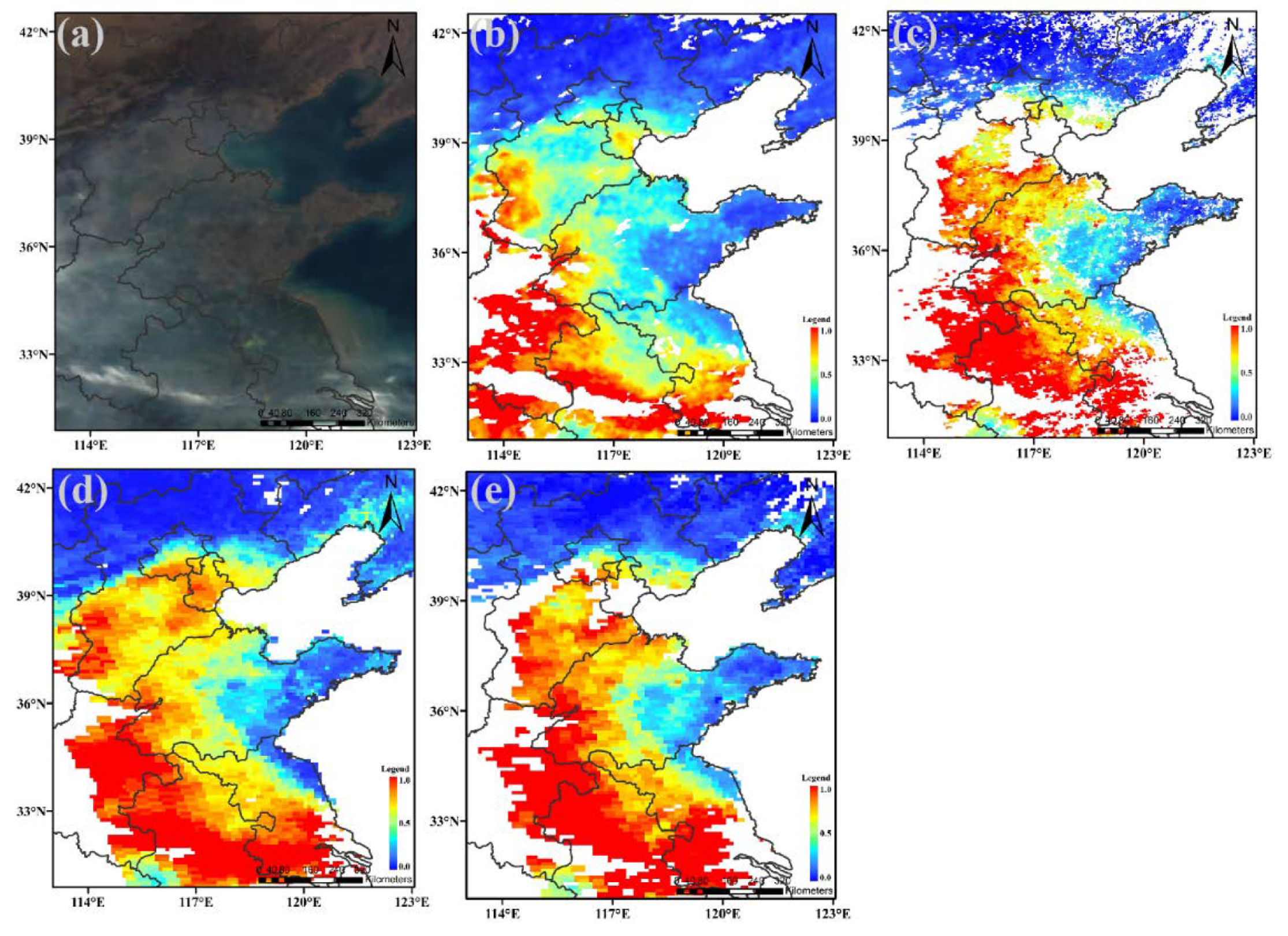
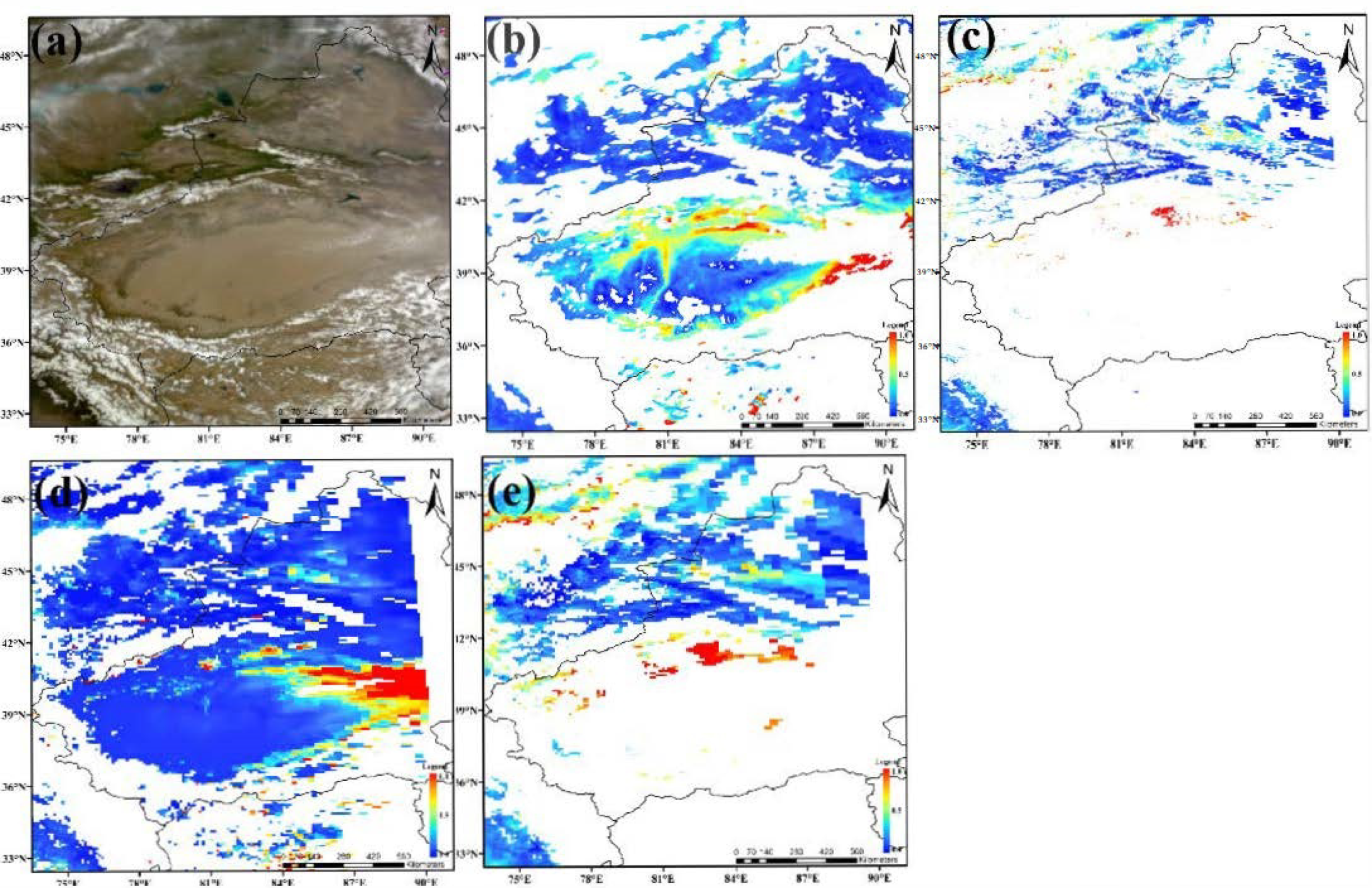
4.1. Case Results over Typical Surface Covers

Figure 6 shows the spatial distribution of the DPC AOD (550 nm) products retrieved from the VISRR on 3 April 2019 over eastern China; the main surface types of this region are grass, croplands, urban land, and water (lake and sea), as shown in Figure 1. Figure 6a is the DPC TOA true-color image (RGB) consisting of $R_{TOA}^{Meas}\left(670\right)$, $R_{TOA}^{Meas}\left(565\right)$, and $R_{TOA}^{Meas}\left(490\right).$ It can be seen that most regions were cloud-free, except for some areas in the south and west, where an obvious strip of white cloud and some flocculent clouds existed; in addition, grey haze aerosols were distributed in most areas and blurred the surface. Figure 6b shows the DPC AOD (3.3 km) products: the blank areas represent those pixels identified as clouds, ice, and water; the blue regions with a low AOD (<0.2) indicate a clean atmosphere and were mainly distributed in the northern and eastern parts of the Shandong peninsula; the slight-pollution ($0.25<$ AOD $<0.5$) regions were spread over southern Beijing–Tianjin–Hebei (BTH), western Shandong, northern Jiangsu, etc.; and moderate- and heavy-pollution regions with a high AOD (>0.5) could be found over most areas of Henan, central Anhui, and southern Jiangsu. Meanwhile, the DPC surface products’ RGB consisting of $R_{SR}\left(670\right)$, $R_{SR}\left(565\right),$ and $R_{SR}\left(490\right)$ is shown in Figure 6c. It can be seen that the surface features became more distinguishable after removing the coupling effect of the atmosphere. In addition, the AOD products of the MYD04_3k_DT AOD (3 km), MYD04_L2_DB AOD (10 km), and MYD04_L2_DT AOD (10 km) results were chosen for comparison and are shown in Figure 6c–e, respectively. Overall, the spatial distribution between the DPC and MODIS AOD products was similar, but there were some differences. First, the AOD from the DPC and MYD04_L2_DB had high spatial coverage. However, the products from MODIS DT were missing in areas such as BTH and the Liaoning region, even if there was no cloud shown in the TOA reflectance RGB. The reason for this might be that the pixels were over-recognized as clouds, or that the DT algorithm cannot be implemented over bright land cover. Second, the spatial resolutions of the DPC and MYD04_3k_DT AOD were 3.3 km (individual pixel) and 3 km, respectively, while that of the MYD04_L2_DT and MYD04_L2_DB AOD was 10 km. In addition to the increased detail, the variations between different gradients of 3.3 or 3 km AOD products are also smoother than those of 10 km products. Third, the four AOD products were of different magnitudes on the whole; the DT AOD products had the highest value, while the DPC products had the lowest value. In this case, the DPC VISRR algorithm can simultaneously retrieve AOD products with the advantages of fine spatial resolution and high coverage.

Figure 7 shows another example of AOD products over western China and its surrounding areas on 30 May 2019, where the main surface types are barren land, grass, permanent snow, ice, and water (lake). From the TOA RGB (a), it can be seen that the permanent snow and ice cover was mainly located in the Himalayas, Kunlun, and the Tianshan Mountains. Thick, thin, and broken clouds were distributed in the Qinghai–Tibet Plateau and east of the Taklimakan Desert. Figure 7b presents the AOD products retrieved from the DPC, which show that the high aerosol loadings were distributed in the oases around the Taklimakan Desert and the Tarim River. Figure 7c–e display the AOD products of MODIS. It is evident that the DT algorithm is ineffective when applied to bright land cover compared to the VISRR and DB products. The DPC AOD products had a higher value over north Taklimakan and were more detailed than the DB products due to their fine spatial resolution.

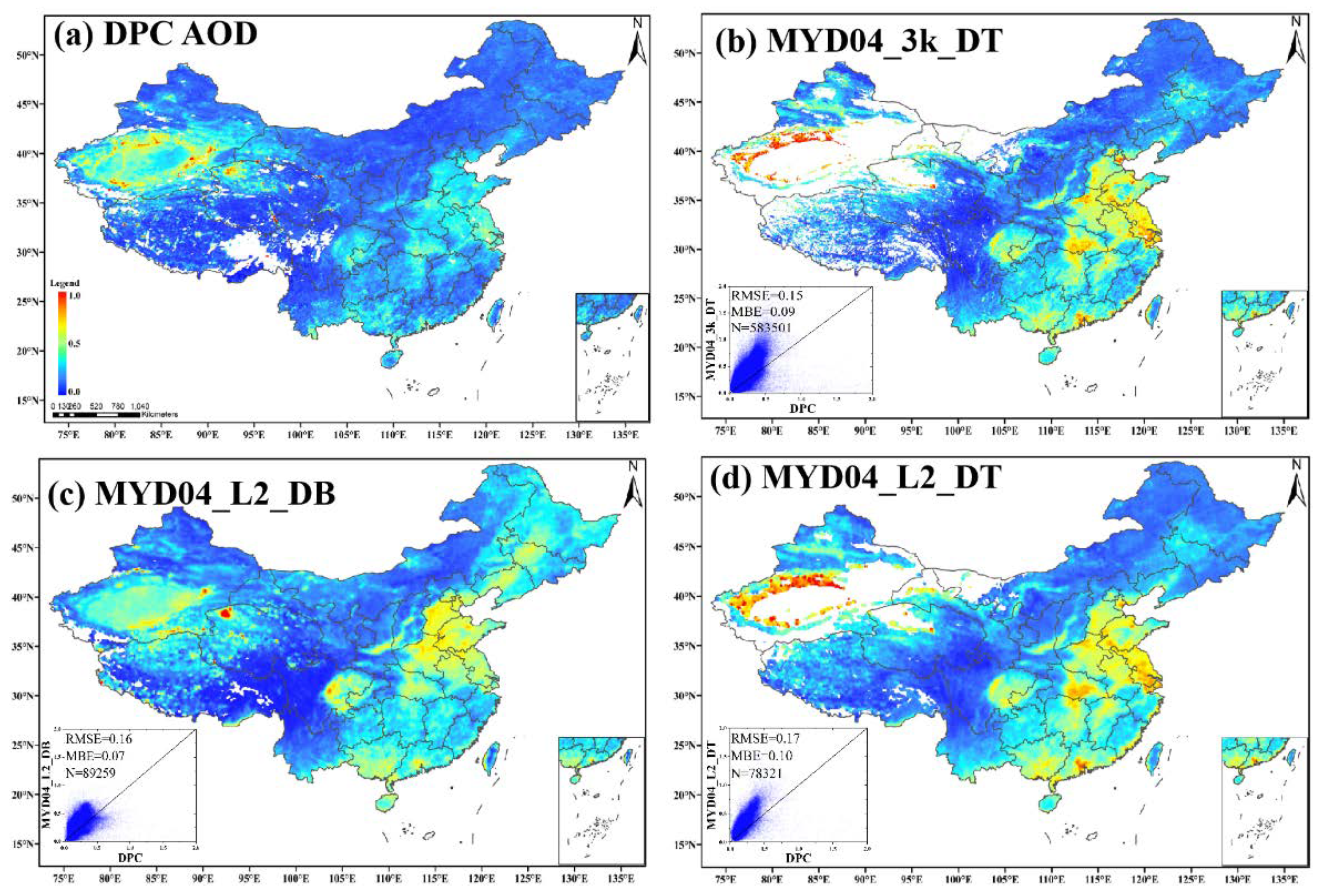
4.2. Average Results over the Study Area

Figure 8a shows the average DPC VISRR AOD products (March 2019 to March 2020) over China. There were four main high-value regions: (1) the northern and eastern plain of China, mainly including BTH, Shandong, Henan, Anhui, and Shanghai, where the aerosol emissions may be related to the fact that this region contains the largest population and the most industries; (2) the Sichuan Basin, mainly including eastern Sichuan and western Chongqing, where, in addition to industrial emissions, topographic and meteorological factors contribute to aerosol pollution [82,83]; (3) southern China, mainly including the south of Yunnan, Guangxi, and Hainan, where smoke aerosol pollution is transported in significant amounts from biomass burning in Southeast Asia [84,85]; (4) western China, mainly including the Taklimakan Desert and its surrounding areas—Taklimakan is the largest desert in China, and dust events often break out here, which are likely responsible for the aerosol pollution over this region [86]. Figure 8b–d present the AOD products from MYD04_3k_DT, MYD04_DB, and MYD04_DT and compare them with the MODIS products. In general, the spatial distributions of the AOD between the DPC and MODIS were similar. However, the AOD magnitude differed in that the MODIS AOD products were slightly higher than those of the DPC over northeastern China and the Qinghai–Tibet Plateau region. According to the validation of He et al. [47], MODIS 3 km and 10 km aerosol products are generally overestimated over China, and the error derives from two main sources. The first is the surface reflectance, and the second is the aerosol models in the LUT.

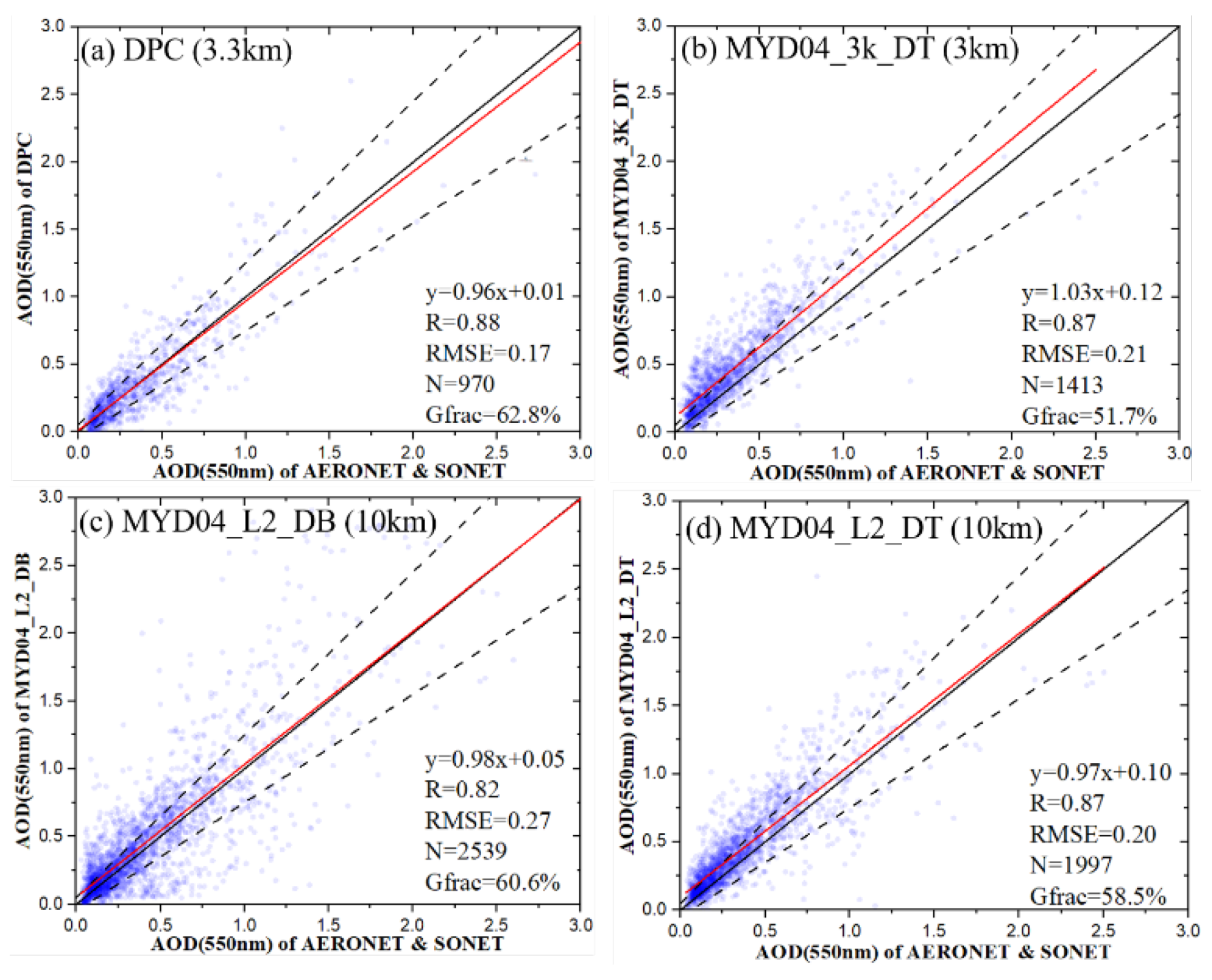
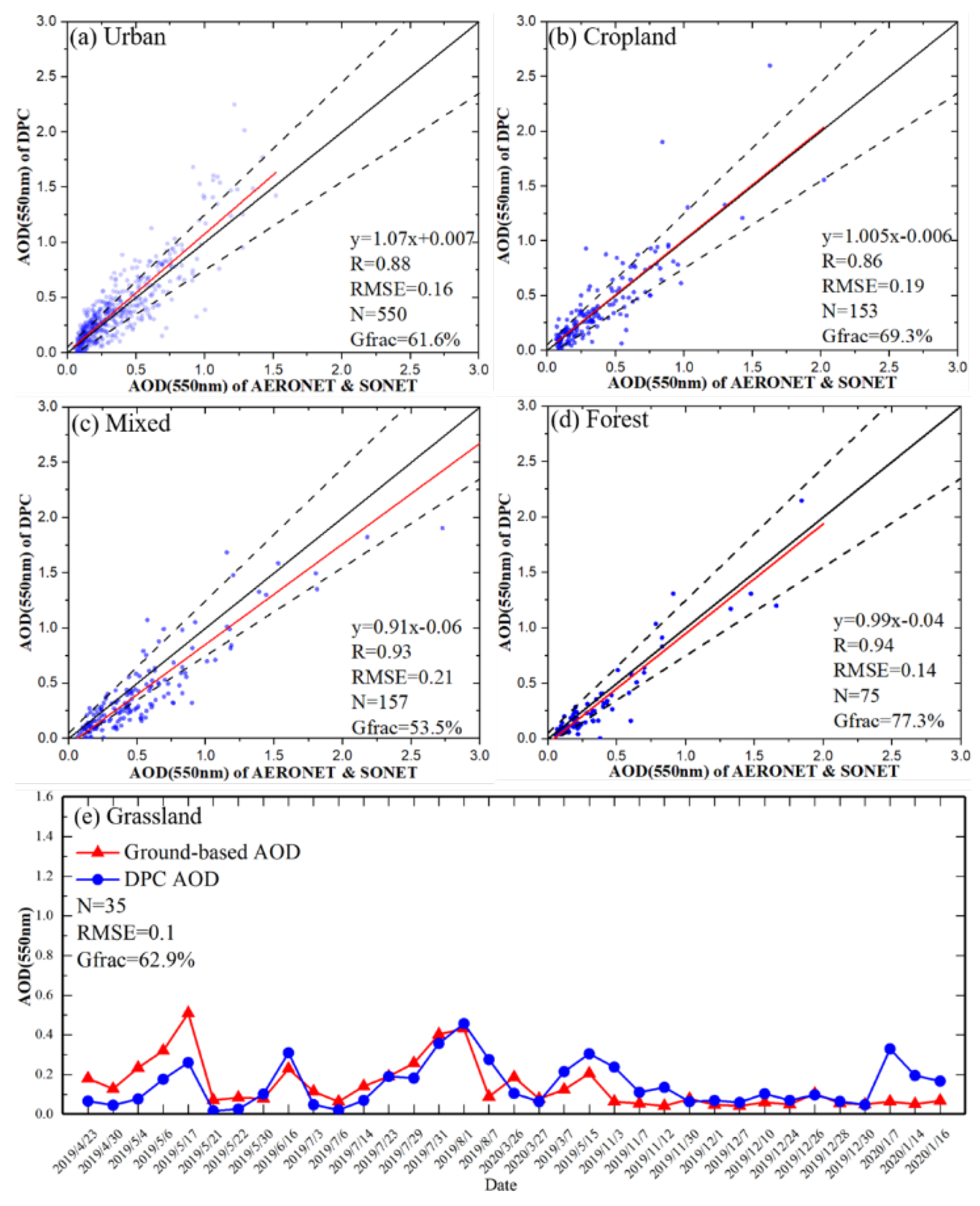
4.3. Validation Using Ground-Based Aerosol Products

In this study, twenty-two AERONET and SONET sites (Figure 1 and Table 2) were chosen to validate the AOD (550 nm) products from the DPC and MODIS. Due to the lack of ground-based measurements with 550 nm AOD products, a second-order polynomial fitting method was chosen to calculate the 550 nm AOD using the 440, 500, and 675 nm values [87]. Furthermore, for the spatiotemporal matching between the ground and the satellites, the ground-based valid AOD products were averaged within one hour (30 min before or after the overpass of the satellite), and the satellite-based available AOD products were averaged within a sampling window (5 $\times$ 5 pixels) centered on the ground site [88]. Figure 9 shows the validation results for the DPC (a) and MODIS (MYD04_3k_DT (b), MYD04_L2_DB (c), and MYD04_L2_DB (d)) AOD products compared to the ground-based products from March 2019 to March 2020. y = a × x + b is a linear fitting equation, where a and b are the slope and intercept, respectively; N is the number of AOD pairs; and the good fraction (Gfrac) refers to the fraction of AOD pairs within the expected error EE = $\pm$(0.05$+$20$\%$). The evaluating indicators of the four aerosol products (a–d) were as follows: a and b were (0.96, 0.01), (1.03, 0.12), (0.98, 0.05), and (0.97, 0.1); the R was 0.88, 0.87, 0.82, and 0.87; the RMSE was 0.17, 0.21, 0.27, and 0.20; the N was 971, 1413, 2539, and 1997; and the Gfrac(s) was 62.7$\%$, 51.7$\%$, 60.6$\%,$ and 58.5$\%$. The best evaluating indicators are presented in bold. The fact that the revisitation period of the DPC was longer than that of MODIS caused the total number of collected DPC AOD retrievals to be the lowest. At the same time, MYD04_L2_DB had the most retrieval results. The slopes of all products were close to 1; however, the DPC AOD products had the lowest intercept and RMSE and the highest R and Gfrac, demonstrating that the DPC AOD products had the highest accuracy over the study area. Specifically, compared with the AOD products at the 3 km level (i.e., Figure 9a versus Figure 9b), although they had a similar R value (0.88 vs. 0.87), the MYD04_3k_DT products had a low Gfrac (51.7$\%$), a slope (1.03) greater than 1, and a high bias of intercept (0.12), revealing that these AOD products were generally overestimated. Compared with the AOD products at the 10 km level (i.e., Figure 9a versus Figure 9c,d), although they had similar Gfrac values (62.7$\%$, 60.6$\%,$ and 58.5$\%$), the MYD04_L2_DB products had a high RMSE (0.27) and a low R (0.82), and the MYD04_L2_DT products were similar to MYD04_3k_DT with a high bias of intercept (0.1). The slope smaller than 1 and the intercept greater than 0 implied that these AOD products were overestimated for small values but underestimated for large values. The validation results of three MODIS AOD products in this study were consistent with previous research [47,54].

To better understand and analyze the uncertainties of the DPC VISRR AOD products, Figure 10 shows the validation results over different land cover types: (a) urban, (b) cropland, (c) mixed, (d) forest, and (e) grassland. The evaluating indicators over the four surface types (a–d) are shown in

Table 9. Statistical parameters of Figure 10a–d. The best evaluating indicators are presented in bold.

Land Cover	a	b	N	R	RMSE	Gfrac
Urban	1.07	0.007	550	0.88	0.16	61.6
Cropland	1.005	−0.006	153	0.86	0.19	69.3
Mixed	0.91	0.11	157	0.93	0.21	53.5
Forest	0.96	−0.06	75	0.94	0.14	77.3

, where the best evaluating indicators are presented in bold. There were 12 ground-based sites covering urban land; therefore, most of the collected DPC AOD retrievals were over this surface type. The slopes and intercepts of all the products were close to 1 and 0; the R was higher than 0.85, and the RMSE was lower than 0.22. Specifically, the accuracy of the DPC AOD over forests and croplands was highest among the surface types, with Gfrac values of 77.3$\%$ and 69.3%, respectively. The reasons for this can be summarized as follows: (1) compared to bright land cover, aerosol retrieval over vegetation (dark) surface types has advantages, as the surface signal accounts for a relatively low proportion of the VIS reflectance at TOA; (2) the VIS SRR with the NDVI and SCA constraints proposed in this study can well express the change in vegetation with time. The Gfrac (61.6$\%$) of urban land was lower than that of forests and croplands, possibly because urban land cover is very complex, consisting of buildings, trees, water, roads, etc., and, with the rapid development of urbanization, urban land cover can change substantially over a short time [89]. Although the VISRR algorithm considers the discrepancies in the SRR over different surface types, it does not consider the change in the surface type over a short period of time, which can result in an estimation error for the surface that can be further transmitted to AOD retrieval. The mixed surface type was represented by three sites (Kashi, Jiaozuo, and Songshan): the Jiaozuo site was mainly a mix of urban land (56%) and cropland (46%); the Songshan site was mainly a mix of forests (36%), grassland (36%), and cropland (28%); and the Kashi site was mainly a mix of barren land (49%), cropland (40%), and grassland (20%). Over mixed-surface-type regions, there will be many mixed pixels. Although these pixels are identified as a certain surface type in advance, the selected prior SRRs may not represent the real relationship of the mixed pixels, which results in retrieval errors. Figure 10e shows the time series of the DPC AOD (blue dot) products against ground-based (red triangle) measurements over grassland (including the AOE_Baotou and Lhasa sites). The first 16 points are matchups from the AOE_Baotou site, and the rest are from the Lhasa site; the evaluating indicators N, RMSE, and Gfrac were 35, 0.1, and 62.9%, respectively. Although most of the valid matched AOD values were lower than 0.2 for AOD_Baotou and 0.1 for Lhasa, it can be seen that DPC AOD products were in better agreement with the ground-based measurements and showed the gradual process of AOD change.

5. Conclusions

In this study, an innovative algorithm called VISRR was proposed and applied to DPC multiangle intensity data to simultaneously retrieve AOD at an intrinsic spatial resolution (3.3 km) over dark and bright land cover. The VISRR algorithm considers surface anisotropy and neither requires a shortwave infrared band nor establishes SRDs. The VISRR’s previous SRRs were built based on long-time-series MYD09 products and consideration of surface types, SCA, and NDVI. Meanwhile, to address the issue of the NDVI being susceptible to the atmosphere, an innovative iterative AC method was proposed to obtain realistic NDVI values. Then, by combining the fundamental aerosol models across China with a LUT method, the proposed algorithm was applied to thirteen months of DPC multiangle intensity data.

A long-time-series comparison and validation of the AOD products were performed, and the results showed that the VISRR algorithm is suitable for dark and bright land cover. The DPC and three MODIS AOD products had similar spatial distribution, but the DPC AOD products had both high spatial resolution and coverage. Validation using twenty-two ground-based sites over different surface types showed that the DPC AOD had the best performance (R of 0.88, RMSE of 0.17, and Gfrac of 62.7$\%$) among the four products over the study area. Then, the uncertainties of the AOD products were comprehensively analyzed and discussed for future improvements. First, the DPC AOD products were validated over five typical surface types: forests had the best Gfrac (77.3$\%$), while mixed land cover had the lowest Gfrac (53.5$\%$). The possible source of error was the chance that the selected prior SRRs did not represent the real relationships of the mixed pixels.

In addition to the DPC/GF-5(01), VISRR can be applied to similar sensors, such as the advanced DPC/GF-5 (02), CM-1, DQ-1, DQ-2, and 3MI [49]. When combined with our previous fine-model aerosol algorithm SNOSPR, based on multiangle polarized data [30], the fine-model aerosol friction can be calculated, a key aerosol optical parameter retrieved from satellite remote sensing for distinguishing aerosol sources.

References

1. Giles, D.M.; Sinyuk, A.; Sorokin, M.G.; Schafer, J.S.; Smirnov, A.; Slutsker, I.; Eck, T.F.; Holben, B.N.; Lewis, J.R.; Campbell, J.R.; et al. Advancements in the Aerosol Robotic Network (AERONET) Version 3 database–automated near-real-time quality control algorithm with improved cloud screening for Sun photometer aerosol optical depth (AOD) measurements. Atmos. Meas. Tech. 2019, 12, 169–209. [Google Scholar] [CrossRef]
2. Li, Z.; Xu, H.; Li, K.; Li, D.; Xie, Y.; Li, L.; Zhang, Y.; Gu, X.; Zhao, W.; Tian, Q. Comprehensive study of optical, physical, chemical and radiative properties of total columnar atmospheric aerosols over China: An overview of Sun-sky radiometer Observation NETwork (SONET) measurements. Bull. Am. Meteor. Soc. 2018, 99, 739–755. [Google Scholar] [CrossRef]
3. Dubovik, O.; Schuster, G.L.; Xu, F.; Hu, Y.; Bösch, H.; Landgraf, J.; Li, Z. Grand Challenges in Satellite Remote Sensing. Front. Remote Sens. 2021, 2, 619818. [Google Scholar] [CrossRef]
4. Griggs, M. Measurements of atmospheric aerosol optical thickness over water using ERTS-1 data. J. Air Pollut. Control. Assoc. 1975, 25, 622–626. [Google Scholar] [CrossRef]
5. Hauser, A.; Oesch, D.; Foppa, N.; Wunderle, S. NOAA AVHRR derived aerosol optical depth over land. J. Geophys. Res. Atmos. 2005, 110, D08204. [Google Scholar] [CrossRef]
6. Von Hoyningen-Huene, W.; Joon, Y.; Vountas, M.; Istomina, G.; Rohen, G.; Dinter, T.; Kokhanovsky, A.; Burrows, J. Retrieval of spectral aerosol optical thickness over land using ocean color sensors MERIS and SeaWiFS. Atmos. Meas. Tech. 2011, 4, 151–171. [Google Scholar] [CrossRef]
7. Jackson, J.M.; Liu, H.; Laszlo, I.; Kondragunta, S.; Remer, L.A.; Huang, J.; Huang, H.C. Suomi-NPP VIIRS aerosol algorithms and data products. J. Geophys. Res. Atmos. 2013, 118, 12673–12689. [Google Scholar] [CrossRef]
8. Kaufman, Y.J.; Sendra, C. Algorithm for automatic atmospheric corrections to visible and near-IR satellite imagery. Int. J. Remote Sens. 1988, 9, 1357–1381. [Google Scholar] [CrossRef]
9. Mei, L.; Rozanov, V.; Vountas, M.; Burrows, J.P.; Richter, A. XBAER-derived aerosol optical thickness from OLCI/Sentinel-3 observation. Atmos. Chem. Phys. 2018, 18, 2511–2523. [Google Scholar] [CrossRef]
10. Garay, M.J.; Witek, M.L.; Kahn, R.A.; Seidel, F.C.; Limbacher, J.A.; Bull, M.A.; Diner, D.J.; Hansen, E.G.; Kalashnikova, O.V.; Lee, H.; et al. Introducing the 4.4 km spatial resolution Multi-Angle Imaging SpectroRadiometer (MISR) aerosol product. Atmos. Meas. Tech. 2020, 13, 593–628. [Google Scholar] [CrossRef]
11. Kolmonen, P.; Sogacheva, L.; Virtanen, T.H.; Leeuw, G.D.; Kulmala, M. The ADV/ASV AATSR aerosol retrieval algorithm: Current status and presentation of a full-mission AOD dataset. Int. J. Digit. Earth 2015, 9, 545–561. [Google Scholar] [CrossRef]
12. Luffarelli, M.; Govaerts, Y.; Franceschini, L. Aerosol Optical Thickness Retrieval in Presence of Cloud: Application to S3A/SLSTR Observations. Atmosphere 2022, 13, 691. [Google Scholar] [CrossRef]
13. Chen, X.; Wang, J.; Liu, Y.; Xu, X.G.; Cai, Z.N.; Yang, D.X.; Yan, C.X.; Feng, L. Angular dependence of aerosol information content in CAPI/TanSat observation over land: Effect of polarization and synergy with A-train satellites. Remote Sens. Environ. 2017, 196, 163–177. [Google Scholar] [CrossRef]
14. Tanré, D.; Bréon, F.; Deuzé, J.; Dubovik, O.; Ducos, F.; François, P.; Goloub, P.; Herman, M.; Lifermann, A.; Waquet, F. Remote sensing of aerosols by using polarized, directional and spectral measurements within the A-Train: The PARASOL mission. Atmos. Meas. Tech. 2011, 4, 1383–1395. [Google Scholar] [CrossRef]
15. Li, Z.; Hou, W.; Hong, J.; Zheng, F.; Luo, D.; Wang, J.; Gu, X.; Qiao, Y. Directional Polarimetric Camera (DPC): Monitoring aerosol spectral optical properties over land from satellite observation. J. Quant. Spectrosc. Radiat. Transf. 2018, 218, 21–37. [Google Scholar] [CrossRef]
16. Sano, I.; Mukai, S.; Nakata, M. An effective method for retrieval of three kinds of aerosol properties focusing on a coming GCOM-C1/SGLI in December of 2017. In Proceedings of the Remote Sensing of Clouds and the Atmosphere XXII, Warsaw, Poland, 13 October 2017; p. 1042403. [Google Scholar]
17. Hsu, N.C.; Tsay, S.-C.; King, M.D.; Herman, J.R. Aerosol properties over bright-reflecting source regions. IEEE Trans. Geosci. Remote Sens. 2004, 42, 557–569. [Google Scholar] [CrossRef]
18. Kaufman, Y.J.; Wald, A.E.; Remer, L.A.; Gao, B.; Li, R.; Flynn, L. The MODIS 2.1-μm channel-correlation with visible reflectance for use in remote sensing of aerosol. IEEE Trans. Geosci. Remote Sens. 1997, 35, 1286–1298. [Google Scholar] [CrossRef]
19. Levy, R.C.; Remer, L.A.; Mattoo, S.; Vermote, E.F.; Kaufman, Y.J. Second-generation operational algorithm: Retrieval of aerosol properties over land from inversion of Moderate Resolution Imaging Spectroradiometer spectral reflectance. J. Geophys. Res. Atmos. 2007, 112, D13211. [Google Scholar] [CrossRef]
20. Hsu, N.; Jeong, M.J.; Bettenhausen, C.; Sayer, A.; Hansell, R.; Seftor, C.; Huang, J.; Tsay, S.C. Enhanced Deep Blue aerosol retrieval algorithm: The second generation. J. Geophys. Res. Atmos. 2013, 118, 9296–9315. [Google Scholar] [CrossRef]
21. Ge, B.; Li, Z.; Liu, L.; Yang, L.; Chen, X.; Hou, W.; Zhang, Y.; Li, D.; Li, L.; Qie, L. A Dark Target Method for Himawari-8/AHI Aerosol Retrieval: Application and Validation. IEEE Trans. Geosci. Remote Sens. 2019, 57, 381–394. [Google Scholar] [CrossRef]
22. Su, X.; Wang, L.; Zhang, M.; Qin, W.; Bilal, M. A High-Precision Aerosol Retrieval Algorithm (HiPARA) for Advanced Himawari Imager (AHI) data: Development and verification. Remote Sens. Environ. 2021, 253, 112221. [Google Scholar] [CrossRef]
23. Gao, L.; Chen, L.; Li, J.; Li, C.; Zhu, L. An improved dark target method for aerosol optical depth retrieval over China from Himawari-8. Atmos. Res. 2021, 250, 105399. [Google Scholar] [CrossRef]
24. Choi, M.; Kim, J.; Lee, J.; Kim, M.; Park, Y.-J.; Jeong, U.; Kim, W.; Hong, H.; Holben, B.; Eck, T.F.; et al. GOCI Yonsei Aerosol Retrieval (YAER) algorithm and validation during the DRAGON-NE Asia 2012 campaign. Atmos. Meas. Tech. 2016, 9, 1377–1398. [Google Scholar] [CrossRef]
25. Zhang, Y.; Li, Z.; Zhang, Y.; Hou, W.; Xu, H.; Chen, C.; Ma, Y. High temporal resolution aerosol retrieval using Geostationary Ocean Color Imager: Application and initial validation. J. Appl. Remote Sens. 2014, 8, 083612. [Google Scholar] [CrossRef]
26. Thomas, G.E.; Carboni, E.; Sayer, A.M.; Poulsen, C.A.; Siddans, R.; Grainger, R.G. Oxford-RAL Aerosol and Cloud (ORAC): Aerosol retrievals from satellite radiometers. In Satellite Aerosol Remote Sensing over Land; Springer: Berlin/Heidelberg, Germany, 2009; pp. 193–225. [Google Scholar]
27. Veefkind, J.P.; de Leeuw, G.; Durkee, P.A. Retrieval of aerosol optical depth over land using two-angle view satellite radiometry during TARFOX. Geophys. Res. Lett. 1998, 25, 3135–3138. [Google Scholar] [CrossRef]
28. Diner, D.J.; Abdou, W.A.; Bruegge, C.J.; Conel, J.E.; Crean, K.A.; Gaitley, B.J.; Helmlinger, M.C.; Kahn, R.A.; Martonchik, J.V.; Pilorz, S.H.; et al. MISR aerosol optical depth retrievals over southern Africa during the SAFARI-2000 Dry Season Campaign. Geophys. Res. Lett. 2001, 28, 3127–3130. [Google Scholar] [CrossRef]
29. Martonchik, J.V.; Kahn, R.A.; Diner, D.J. Retrieval of aerosol properties over land using MISR observations. In Satellite Aerosol Remote Sensing over Land; Springer: Berlin/Heidelberg, Germany, 2009; pp. 267–293. [Google Scholar]
30. Ge, B.; Mei, X.; Li, Z.; Hou, W.; Xie, Y.; Zhang, Y.; Xu, H.; Li, K.; Wei, Y. An improved algorithm for retrieving high resolution fine-mode aerosol based on polarized satellite data: Application and validation for POLDER-3. Remote Sens. Environ. 2020, 247, 111894. [Google Scholar] [CrossRef]
31. Dubovik, O.; Herman, M.; Holdak, A.; Lapyonok, T.; Tanré, D.; Deuzé, J.; Ducos, F.; Sinyuk, A.; Lopatin, A. Statistically optimized inversion algorithm for enhanced retrieval of aerosol properties from spectral multi-angle polarimetric satellite observations. Atmos. Meas. Tech. 2011, 4, 975–1018. [Google Scholar] [CrossRef]
32. Chen, C.; Dubovik, O.; Fuertes, D.; Litvinov, P.; Lapyonok, T.; Lopatin, A.; Ducos, F.; Derimian, Y.; Herman, M.; Tanré, D.; et al. Validation of GRASP algorithm product from POLDER/PARASOL data and assessment of multi-angular polarimetry potential for aerosol monitoring. Earth Syst. Sci. Data 2020, 12, 3573–3620. [Google Scholar] [CrossRef]
33. Wei, Y.; Li, Z.; Zhang, Y.; Chen, C.; Dubovik, O.; Zhang, Y.; Xu, H.; Li, K.; Chen, J.; Wang, H.; et al. Validation of POLDER GRASP Aerosol Optical Retrieval Over China Using SONET Observations. J. Quant. Spectrosc. Radiat. Transf. 2020, 246, 106931. [Google Scholar] [CrossRef]
34. Dubovik, O.; Holben, B.; Eck, T.F.; Smirnov, A.; Kaufman, Y.J.; King, M.D.; Tanré, D.; Slutsker, I. Variability of absorption and optical properties of key aerosol types observed in worldwide locations. J. Atmos. Sci. 2002, 59, 590–608. [Google Scholar] [CrossRef]
35. Omar, A.H.; Won, J.G.; Winker, D.M.; Yoon, S.C.; Dubovik, O.; McCormick, M.P. Development of global aerosol models using cluster analysis of Aerosol Robotic Network (AERONET) measurements. J. Geophys. Res. Atmos. 2005, 110, D10S14. [Google Scholar] [CrossRef]
36. Levy, R.C.; Remer, L.A.; Dubovik, O. Global aerosol optical properties and application to Moderate Resolution Imaging Spectroradiometer aerosol retrieval over land. J. Geophys. Res. Atmos. 2007, 112, D13210. [Google Scholar] [CrossRef]
37. Lee, J.; Kim, J.; Song, C.; Kim, S.; Chun, Y.; Sohn, B.; Holben, B. Characteristics of aerosol types from AERONET sunphotometer measurements. Atmos. Environ. 2010, 44, 3110–3117. [Google Scholar] [CrossRef]
38. Mei, L.; Rozanov, V.; Vountas, M.; Burrows, J.P.; Levy, R.C.; Lotz, W. Retrieval of aerosol optical properties using MERIS observations: Algorithm and some first results. Remote Sens. Environ. 2017, 197, 125–140. [Google Scholar] [CrossRef]
39. Omar, A.H.; Winker, D.M.; Vaughan, M.A.; Hu, Y.; Trepte, C.R.; Ferrare, R.A.; Lee, K.-P.; Hostetler, C.A.; Kittaka, C.; Rogers, R.R.; et al. The CALIPSO automated aerosol classification and lidar ratio selection algorithm. J. Atmos. Ocean. Technol. 2009, 26, 1994–2014. [Google Scholar] [CrossRef]
40. Li, Z.; Zhang, Y.; Xu, H.; Li, K.; Dubovik, O.; Goloub, P. The Fundamental Aerosol Models Over China Region: A Cluster Analysis of the Ground-Based Remote Sensing Measurements of Total Columnar Atmosphere. Geophys. Res. Lett. 2019, 46, 4924–4932. [Google Scholar] [CrossRef]
41. Levy, R.; Mattoo, S.; Munchak, L.; Remer, L.; Sayer, A.; Patadia, F.; Hsu, N. The Collection 6 MODIS aerosol products over land and ocean. Atmos. Meas. Tech. 2013, 6, 2989–3034. [Google Scholar] [CrossRef]
42. Sayer, A.M.; Hsu, N.C.; Lee, J.; Kim, W.V.; Dutcher, S.T. Validation, stability, and consistency of MODIS Collection 6.1 and VIIRS Version 1 Deep Blue aerosol data over land. J. Geophys. Res. Atmos. 2019, 124, 4658–4688. [Google Scholar] [CrossRef]
43. Tao, M.; Wang, J.; Li, R.; Chen, L.; Xu, X.; Wang, L.; Tao, J.; Wang, Z.; Xiang, J. Characterization of aerosol type over East Asia by 4.4 km MISR product: First insight and general performance. J. Geophys. Res. Atmos. 2020, 125, e2019JD031909. [Google Scholar] [CrossRef]
44. Li, C.; Li, J.; Xu, H.; Li, Z.; Xia, X.; Che, H. Evaluating VIIRS EPS Aerosol Optical Depth in China: An intercomparison against ground-based measurements and MODIS. J. Quant. Spectrosc. Radiat. Transf. 2019, 224, 368–377. [Google Scholar] [CrossRef]
45. Wei, J.; Sun, L.; Huang, B.; Bilal, M.; Zhang, Z.; Wang, L. Verification, improvement and application of aerosol optical depths in China Part 1: Inter-comparison of NPP-VIIRS and Aqua-MODIS. Atmos. Environ. 2018, 175, 221–233. [Google Scholar] [CrossRef]
46. Sogacheva, L.; de Leeuw, G.; Rodriguez, E.; Kolmonen, P.; Georgoulias, A.K.; Alexandri, G.; Kourtidis, K.; Proestakis, E.; Marinou, E.; Amiridis, V. Spatial and seasonal variations of aerosols over China from two decades of multi-satellite observations–part 1: ATSR (1995–2011) and MODIS C6. 1 (2000–2017). Atmos. Chem. Phys. 2018, 18, 11389–11407. [Google Scholar] [CrossRef]
47. He, Q.; Zhang, M.; Huang, B.; Tong, X. MODIS 3 km and 10 km aerosol optical depth for China: Evaluation and comparison. Atmos. Environ. 2017, 153, 150–162. [Google Scholar] [CrossRef]
48. Huang, G.; Chen, Y.; Li, Z.; Liu, Q.; Wang, Y.; He, Q.; Liu, T.; Liu, X.; Zhang, Y.; Gao, J. Validation and Accuracy Analysis of the Collection 6.1 MODIS Aerosol Optical Depth Over the Westernmost City in China Based on the Sun-Sky Radiometer Observations From SONET. Earth Space Sci. 2020, 7, e2019EA001041. [Google Scholar] [CrossRef]
49. Dubovik, O.; Li, Z.; Mishchenko, M.I.; Tanré, D.; Karol, Y.; Bojkov, B.; Cairns, B.; Diner, D.J.; Espinosa, W.R.; Goloub, P.; et al. Polarimetric remote sensing of atmospheric aerosols: Instruments, methodologies, results, and perspectives. J. Quant. Spectrosc. Radiat. Transf. 2018, 224, 474–511. [Google Scholar] [CrossRef]
50. Friedl, M.A.; Sulla-Menashe, D.; Tan, B.; Schneider, A.; Ramankutty, N.; Sibley, A.; Huang, X. MODIS Collection 5 global land cover: Algorithm refinements and characterization of new datasets. Remote Sens. Environ. 2010, 114, 168–182. [Google Scholar] [CrossRef]
51. Zhu, S.; Li, Z.; Qie, L.; Xu, H.; Ge, B.; Xie, Y.; Qiao, R.; Xie, Y.; Hong, J.; Meng, B.; et al. In-Flight Relative Radiometric Calibration of a Wide Field of View Directional Polarimetric Camera Based on the Rayleigh Scattering over Ocean. Remote Sens. 2022, 14, 1211. [Google Scholar] [CrossRef]
52. Danielson, J.J.; Gesch, D.B. Global Multi-Resolution Terrain Elevation Data 2010 (GMTED2010). US Department of the Interior; US Geological Survey, 2011. Available online: https://pubs.usgs.gov/of/2011/1073/ (accessed on 15 August 2022).
53. Kokaly, R.; Clark, R.; Swayze, G.; Livo, K.; Hoefen, T.; Pearson, N.; Wise, R.; Benzel, W.; Lowers, H.; Driscoll, R.; et al. Usgs Spectral Library Version 7 Data: Us Geological Survey Data Release; United States Geological Survey (USGS): Reston, VA, USA, 2017. [Google Scholar] [CrossRef]
54. Liu, N.; Zou, B.; Feng, H.; Tang, Y.; Liang, Y. Evaluation and comparison of MAIAC, DT and DB aerosol products over China. Atmos. Chem. Phys. Discuss 2019, 19, 8243–8268. [Google Scholar] [CrossRef]
55. Li, X.; Strahler, A.H. Geometric-optical bidirectional reflectance modeling of the discrete crown vegetation canopy: Effect of crown shape and mutual shadowing. IEEE Trans. Geosci. Remote Sens. 1992, 30, 276–292. [Google Scholar] [CrossRef]
56. Lucht, W.; Schaaf, C.B.; Strahler, A.H. An algorithm for the retrieval of albedo from space using semiempirical BRDF models. IEEE Trans. Geosci. Remote Sens. 2000, 38, 977–998. [Google Scholar] [CrossRef]
57. Jiao, Z.; Ding, A.; Kokhanovsky, A.; Schaaf, C.; Bréon, F.-M.; Dong, Y.; Wang, Z.; Liu, Y.; Zhang, X.; Yin, S.; et al. Development of a snow kernel to better model the anisotropic reflectance of pure snow in a kernel-driven BRDF model framework. Remote Sens. Environ. 2019, 221, 198–209. [Google Scholar] [CrossRef]
58. Bréon, F.-M.; Vermote, E. Correction of MODIS surface reflectance time series for BRDF effects. Remote Sens. Environ. 2012, 125, 1–9. [Google Scholar] [CrossRef]
59. Schaaf, C.B.; Gao, F.; Strahler, A.H.; Lucht, W.; Li, X.; Tsang, T.; Strugnell, N.C.; Zhang, X.; Jin, Y.; Muller, J.-P.; et al. First operational BRDF, albedo nadir reflectance products from MODIS. Remote Sens. Environ. 2002, 83, 135–148. [Google Scholar] [CrossRef]
60. Liu, Y.; Wang, Z.; Sun, Q.; Erb, A.M.; Li, Z.; Schaaf, C.B.; Zhang, X.; Román, M.O.; Scott, R.L.; Zhang, Q.; et al. Evaluation of the VIIRS BRDF, Albedo and NBAR products suite and an assessment of continuity with the long term MODIS record. Remote Sens. Environ. 2017, 201, 256–274. [Google Scholar] [CrossRef]
61. Wanner, W.; Li, X.; Strahler, A. On the derivation of kernels for kernel-driven models of bidirectional reflectance. J. Geophys. Res. Atmos. 1995, 100, 21077–21089. [Google Scholar] [CrossRef]
62. Vermote, E.; Justice, C.O.; Bréon, F.-M. Towards a generalized approach for correction of the BRDF effect in MODIS directional reflectances. IEEE Trans. Geosci. Remote Sens. 2009, 47, 898–908. [Google Scholar] [CrossRef]
63. Yang, L.; Xue, Y.; Li, Y.; Li, C.; Guang, J.; He, X.; Dong, J.; Hou, T. Uncertainty from Lambertian surface assumption in satellite aerosol retrieval. In Proceedings of the 2012 IEEE International Geoscience and Remote Sensing Symposium, Munich, Germany, 22–27 July 2012; pp. 3662–3665. [Google Scholar]
64. Qin, W.; Herman, J.R.; Ahmad, Z. A fast, accurate algorithm to account for non-Lambertian surface effects on TOA radiance. J. Geophys. Res. Atmos. 2001, 106, 22671–22684. [Google Scholar] [CrossRef]
65. She, L.; Xue, Y.; Yang, X.; Leys, J.; Guang, J.; Che, Y.; Fan, C.; Xie, Y.; Li, Y. Joint Retrieval of Aerosol Optical Depth and Surface Reflectance Over Land Using Geostationary Satellite Data. IEEE Trans. Geosci. Remote Sens. 2018, 57, 1489–1501. [Google Scholar] [CrossRef]
66. Yang, L.; Xue, Y.; Guang, J.; Kazemian, H.; Zhang, J.; Li, C. Improved Aerosol Optical Depth and Ångstrom Exponent Retrieval Over Land From MODIS Based on the Non-Lambertian Forward Model. IEEE Geosci. Remote Sens. Lett. 2014, 11, 1629–1633. [Google Scholar] [CrossRef]
67. He, T.; Liang, S.; Wang, D.; Wu, H.; Yu, Y.; Wang, J. Estimation of surface albedo and directional reflectance from Moderate Resolution Imaging Spectroradiometer (MODIS) observations. Remote Sens. Environ. 2012, 119, 286–300. [Google Scholar] [CrossRef]
68. Koelemeijer, R.; De Haan, J.; Stammes, P. A database of spectral surface reflectivity in the range 335–772 nm derived from 5.5 years of GOME observations. J. Geophys. Res. Atmos. 2003, 108, 4070. [Google Scholar] [CrossRef]
69. Sun, L.; Wei, J.; Bilal, M.; Tian, X.; Jia, C.; Guo, Y.; Mi, X. Aerosol optical depth retrieval over bright areas using Landsat 8 OLI images. Remote Sens. 2016, 8, 23. [Google Scholar] [CrossRef]
70. Sayer, A.M.; Thomas, G.E.; Grainger, R.G.; Carboni, E.; Poulsen, C.; Siddans, R. Use of MODIS-derived surface reflectance data in the ORAC-AATSR aerosol retrieval algorithm: Impact of differences between sensor spectral response functions. Remote Sens. Environ. 2012, 116, 177–188. [Google Scholar] [CrossRef]
71. Wang, Z.; Deng, R.; Ma, P.; Zhang, Y.; Liang, Y.; Chen, H.; Zhao, S.; Chen, L. 250-m Aerosol Retrieval from FY-3 Satellite in Guangzhou. Remote Sens. 2021, 13, 920. [Google Scholar] [CrossRef]
72. Qie, L.; Ma, Y.; Chen, X.; Li, L.; Li, Z.; Zhang, Y. Aerosol model assumption: The retrievals of aerosol optical depth from satellite near-infrared polarimetric measurements. J. Infrared Millim. Waves 2016, 35, 569–577. [Google Scholar]
73. Vermote, E.; Tanré, D.; Deuzé, J.; Herman, M.; Morcrette, J.; Kotchenova, S. Second Simulation of a Satellite Signal in the Solar Spectrum-Vector (6SV). Available online: https://salsa.umd.edu/files/6S/6S_Manual_Part_1.pdf (accessed on 30 July 2022).
74. Levy, R.C.; Remer, L.A.; Tanré, D.; Mattoo, S.; Kaufman, Y.J. Algorithm for Remote Sensing of Tropospheric Aerosol over Dark Targets from MODIS: Collections 005 and 051: Revision 2. February 2009. Available online: https://citeseerx.ist.psu.edu/viewdoc/download?doi=10.1.1.386.980&rep=rep1&type=pdf (accessed on 30 July 2022).
75. Fraser, R.S.; Ferrare, R.A.; Kaufman, Y.J.; Markham, B.L.; Mattoo, S. Algorithm for atmospheric corrections of aircraft and satellite imagery. Int. J. Remote Sens. 1992, 13, 541–557. [Google Scholar] [CrossRef]
76. Deuzé, J.; Bréon, F.; Devaux, C.; Goloub, P.; Herman, M.; Lafrance, B.; Maignan, F.; Marchand, A.; Nadal, F.; Perry, G.; et al. Remote sensing of aerosols over land surfaces from POLDER-ADEOS-1 polarized measurements. J. Geophys. Res. Atmos. 2001, 106, 4913–4926. [Google Scholar] [CrossRef]
77. Von Hoyningen-Huene, W.; Freitag, M.; Burrows, J. Retrieval of aerosol optical thickness over land surfaces from top-of-atmosphere radiance. J. Geophys. Res. Atmos. 2003, 108, 4260. [Google Scholar] [CrossRef]
78. She, L.; Mei, L.; Xue, Y.; Che, Y.; Guang, J. SAHARA: A Simplified AtmospHeric Correction AlgoRithm for Chinese gAofen Data: 1. Aerosol Algorithm. Remote Sens. 2017, 9, 253. [Google Scholar] [CrossRef]
79. Ge, B.; Li, Z.; Hou, W.; Ma, Y.; Xie, Y.; Wang, H.; Zhu, S.; Chen, J. An impact study of NDVI on the BPDF model under different atmosphere and multi-angles conditions. In Proceedings of the Applied Optics and Photonics China (AOPC2019), Nanjing, China, 22 December 2019; p. 1133834. [Google Scholar]
80. Liu, G.; Liang, C.; Kuo, T.; Lin, T.; Huang, S. Comparison of the NDVI, ARVI and AFRI Vegetation Index, Along with Their Relations with the AOD Using SPOT 4 Vegetation Data. Terr. Atmos. Ocean. Sci. 2004, 15, 15–31. [Google Scholar] [CrossRef]
81. Nagol, J.R.; Vermote, E.F.; Prince, S.D. Effects of atmospheric variation on AVHRR NDVI data. Remote Sens. Environ. 2009, 113, 392–397. [Google Scholar] [CrossRef]
82. Zhang, C.; Zhang, Y.; Li, Z.; Wang, Y.; Xu, H.; Li, K.; Li, D.; Xie, Y.; Zhang, Y. Sub-Mode Aerosol Volume Size Distribution and Complex Refractive Index from the Three-Year Ground-Based Measurements in Chengdu China. Atmosphere 2019, 10, 46. [Google Scholar] [CrossRef]
83. Liu, X.; Chen, Q.; Che, H.; Zhang, R.; Gui, K.; Zhang, H.; Zhao, T. Spatial distribution and temporal variation of aerosol optical depth in the Sichuan basin, China, the recent ten years. Atmos. Environ. 2016, 147, 434–445. [Google Scholar] [CrossRef]
84. Zhu, J.; Xia, X.; Wang, J.; Zhang, J.; Wiedinmyer, C.; Fisher, J.A.; Keller, C.A. Impact of Southeast Asian smoke on aerosol properties in Southwest China: First comparison of model simulations with satellite and ground observations. J. Geophys. Res. Atmos. 2017, 122, 3904–3919. [Google Scholar] [CrossRef]
85. Shao, P.; Xin, J.; Zhang, X.; Gong, C.; Ma, Y.; Wang, Y.; Wang, S.; Hu, B.; Ren, X.; Wang, B. Aerosol optical properties and their impacts on the co–occurrence of surface ozone and particulate matter in Kunming City, on the Yunnan–Guizhou Plateau of China. Atmos. Res. 2022, 266, 105963. [Google Scholar] [CrossRef]
86. Huang, J.; Minnis, P.; Chen, B.; Huang, Z.; Liu, Z.; Zhao, Q.; Yi, Y.; Ayers, J.K. Long-range transport and vertical structure of Asian dust from CALIPSO and surface measurements during PACDEX. J. Geophys. Res. Atmos. 2008, 113, D23212. [Google Scholar] [CrossRef]
87. Eck, T.; Holben, B.; Reid, J.; Dubovik, O.; Smirnov, A.; O’neill, N.; Slutsker, I.; Kinne, S. Wavelength dependence of the optical depth of biomass burning, urban, and desert dust aerosols. J. Geophys. Res. Atmos. 1999, 104, 31333–31349. [Google Scholar] [CrossRef]
88. Remer, L.A.; Mattoo, S.; Levy, R.C.; Munchak, L.A. MODIS 3 km aerosol product: Algorithm and global perspective. Atmos. Meas. Tech. 2013, 6, 1829–1844. [Google Scholar] [CrossRef]
89. Zhang, H.; Wang, T.; Zhang, Y.; Dai, Y.; Jia, J.; Yu, C.; Li, G.; Lin, Y.; Lin, H.; Cao, Y. Quantifying short-term urban land cover change with time series landsat data: A comparison of four different cities. Sensors 2018, 18, 4319. [Google Scholar] [CrossRef]
Figure 1. Land cover types of the study area and locations of AERONET (yellow stars) and SONET (blue stars) sites.
Remotesensing 14 04045 g001
Figure 2. SRFs of DPC (red dotted line) and MODIS (gray dotted line), from left to right, are 443, 490, 565, 670, and 865 nm. The solid lines show the spectral reflectance of typical surface materials in Splib07b, i.e., blackbrush, sand, brick, and acmite, representing vegetation, soil, artificial material, and minerals, respectively. The abscissa represents the wavelength, the left ordinate represents the spectral response function value, and the right represents the surface reflectance value.
Remotesensing 14 04045 g002
Figure 3. Relationship between SR calculated for DPC 490 and that calculated for 670 nm (a) and 865 nm (b). The differently colored dots represent different surface materials.
Remotesensing 14 04045 g003
Figure 4. SRRs between DPC (a) 443 and (b) 490 versus 670 nm, respectively. The serial numbers (1)–(16) of each subgraph (except for (15) permanent snow and ice and (17) water) represent different surface types, as shown in Figure 1. The abscissa represents the SR of 670 nm, and the ordinate represents (a) 443 and (b) 490 nm, respectively. The color bar represents the NDVI value.
Remotesensing 14 04045 g004
Figure 5. Flowchart of the main steps of the VISRR aerosol and surface retrieval algorithm.
Remotesensing 14 04045 g005
Figure 6. AOD (550 nm) distribution on 3 April 2019: (a) DPC true-color image (670,565 and 490 nm) of TOA, (b) DPC AOD (3.3 km) results from VISRR, (c) AOD (3 km) results from MYD04_3k_DT, (d) AOD (10 km) results from MYD04_L2_DB, (e) AOD (10 km) results from MYD04_L2_DT.
Remotesensing 14 04045 g006
Figure 7. AOD (550 nm) distribution on 30 May 2019: (a) DPC true-color image (670,565 and 490 nm) of TOA, (b) DPC AOD (3.3 km) results from VISRR, (c) AOD (3 km) results from MYD04_3k_DT, (d) AOD (10 km) results from MYD04_L2_DB, (e) AOD (10 km) results from MYD04_L2_DT.
Remotesensing 14 04045 g007
Figure 8. Spatial distribution of average AOD products from March 2019 to March 2020. (a) DPC AOD (3.3 km) products from VISRR, (b) AOD (3 km) results from MYD04_3k_DT, (c) AOD (10 km) results from MYD04_L2_DB, (d) AOD (10 km) results from MYD04_L2_DT. The scatter plots on the bottom left of subgraph (b,c) show the comparison between DPC and MODIS AOD products, based on the spatial interpolation of DPC data. The RMSEs between DPC and MYD04_3k_DT, MYD04_L2_DB, and MYD04_L2_DT were 0.15, 0.16, and 0.17, and the mean bias errors (MBEs) were 0.09, 0.07, and 0.10, respectively.
Remotesensing 14 04045 g008
Figure 9. Validation of AOD (550 nm) products between ground-based and satellite-based measurements: (a) DPC (3.3 km), (b) MYD04_3k (3 km), (c) MYD04_L2_DB (10 km), and (d) MYD04_L2_DT (10 km). Black solid and dashed lines are the 1:1 lines and EE ( ± (0.05 + 20 % ) envelope lines, respectively. Blue dots and red fitting lines represent the satellite-based and ground-based measurements, respectively.
Remotesensing 14 04045 g009
Figure 10. Validation of DPC AOD (550 nm) products against ground-based measurements over different surface types: (a) urban, (b) cropland, (c) mixed, (d) forest, and (e) grassland. Blue dots and red triangles represent the DPC AOD and ground-based measurements.
Remotesensing 14 04045 g010