
Performance Analysis of Relay-Aided NOMA Optical Wireless Communication System in Underwater Turbulence Environment


Abstract
:
1. Introduction
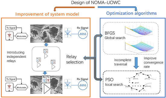
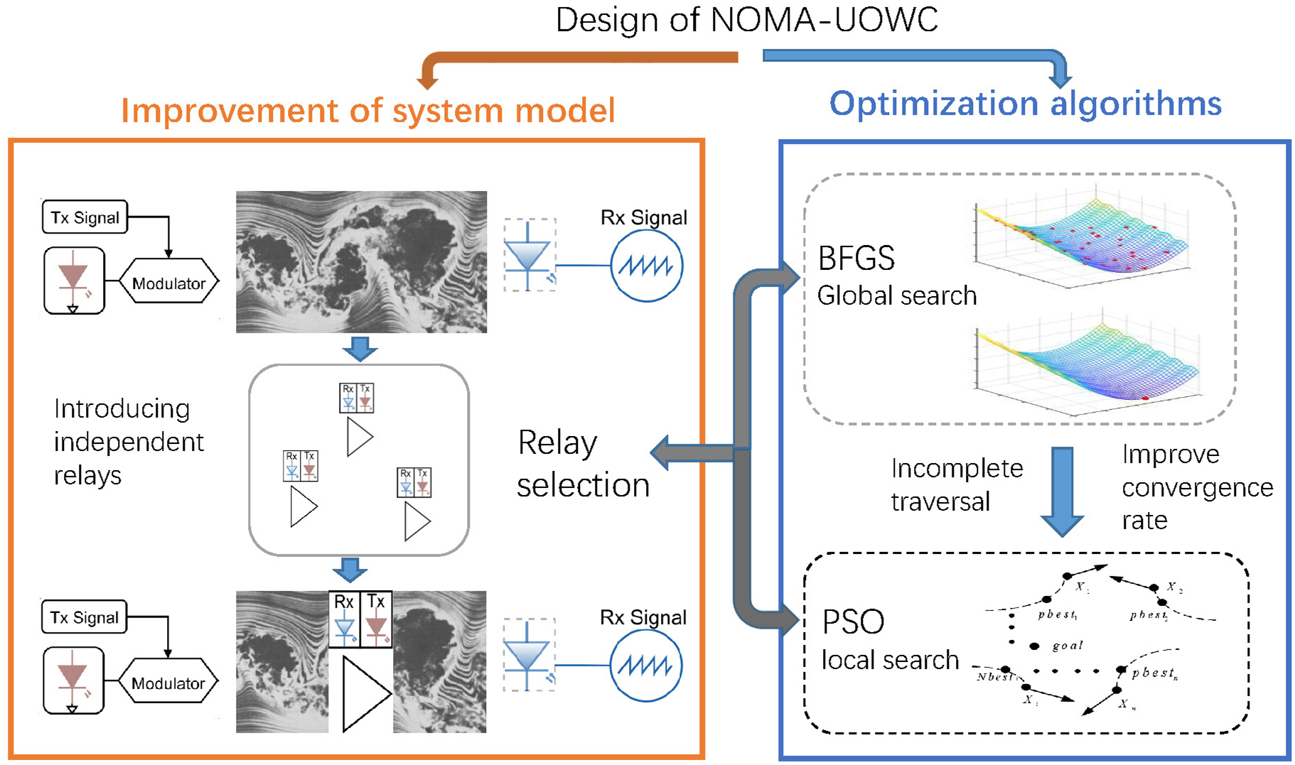
2. System Model
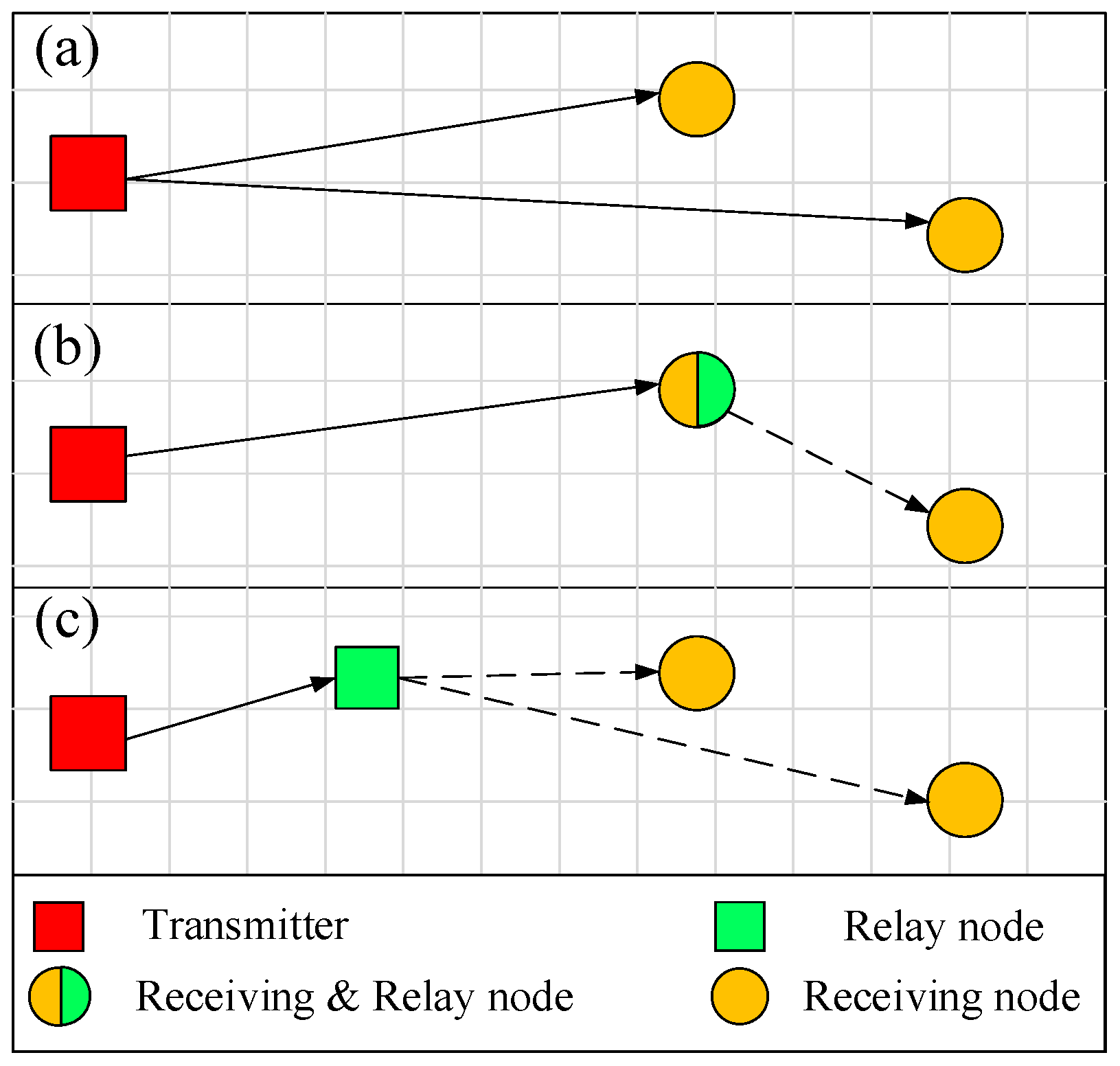
3. User Pairing Scheme Jointed with Relay Selection
4. Sum Rate-Based Power Optimization
4.1. Fixed Power Allocation Method
| Algorithm 1 Fixed Power Allocation Algorithm |
| Initialize Power allocation ratio ξ1 = 0, step factor Δξ, the total transmitted power of system Ptotal, the number of relay nodes M. Output: The power allocation ratioζ, the sum rates Rtotal. 1: Initialize smax = [1/Δξ], , Rtotal = 0, ζ[]. 2: for m = 1→M do 3: Determine NOMA pairing nodes i and j according to (11)~(13) 4: for s = 1→smax do 5: ξ#= ξs + Δξ 6: Compute according to (14b), (14c) 7: Compute according to (9) and (10) 8: 9: if then 10: , ξm = ξ# 11: else 12: s = s + 1 13: end if 14: end for 15: 16: ζ(m)= ξm 17: end for |
4.2. Global Optimal Power Allocation
| Algorithm 2 Global Optimal Power Allocation Optimization |
| Initialize Target rate Rth, maximum iterations smax, the precision threshold τ, the total transmitted power of system Ptotal, the number of relay nodes M. Output: . . 2: for s = 1→smax do 3: Determine the search direction 4: d(s) = −(B(s))−1 × g(s) 5: Compute the step factor ϖ(s) according to (20) 6: Compute the mark vector 7: q(s) = l(s)d(s), P(s+1) = P(s)+ q(s) 6: Compute ||g(s+1)||2 7: if ||g(s+1)||2 < τ then 8: break according to (9) and (10) then 12: Compute p(s) = g(s+1) − g(s) according to (25) 13: Compute B(s+1) = B(s) + ΔB(s) according to (27) 14: Let s = s + 1 and return to step 3 15: else break 16: end if 17: end if 18: end for |
4.3. Stepwise Sub-Optimization Power Allocation
| Algorithm 3 Stepwise Sub-Optimization Power Allocation |
| Step 1 Compute the power allocation coefficient of pairing nodes according to (26) Step 2 Optimize the power allocation between transmitter and relay node Initialize ←0. Output: . 1: for k ←1 to K 2: Initialize the initial source node transmission power factor ck and the velocity factor vk. according to (9) and (10) then 6: pbest(k) ← c(k), gbest ← 7: else break 8: end if 9: end for 10: while not stop 11: fors ← 1 to smax 12: Update the source node transmission power factor c(k) and the velocity factor v(k) according to (31) and (32) 13: if fit(c(k)) > fit(pbest(k)) then 14: pbest(k) ← c(k) 15: if fit(pbest(k)) > fit(gbest) then 16: gbest ← pbest(k) 17: end for 19: end while |
4.4. Analysis of Algorithm Complexity
5. Simulation and Analysis
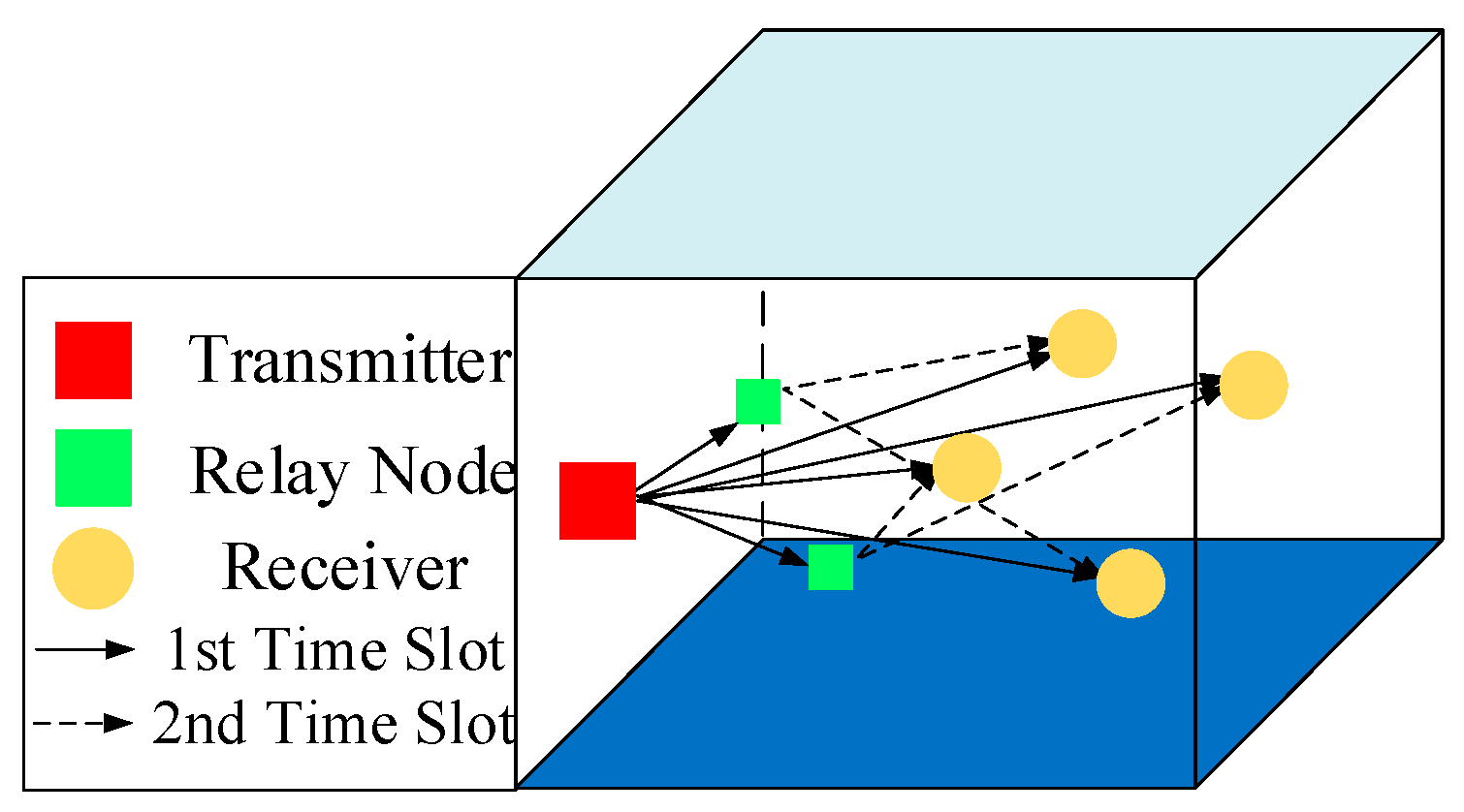
5.1. Simulation Scenarios for NOMA–UOWC Network
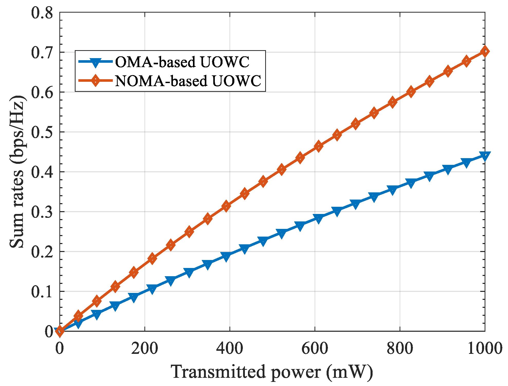
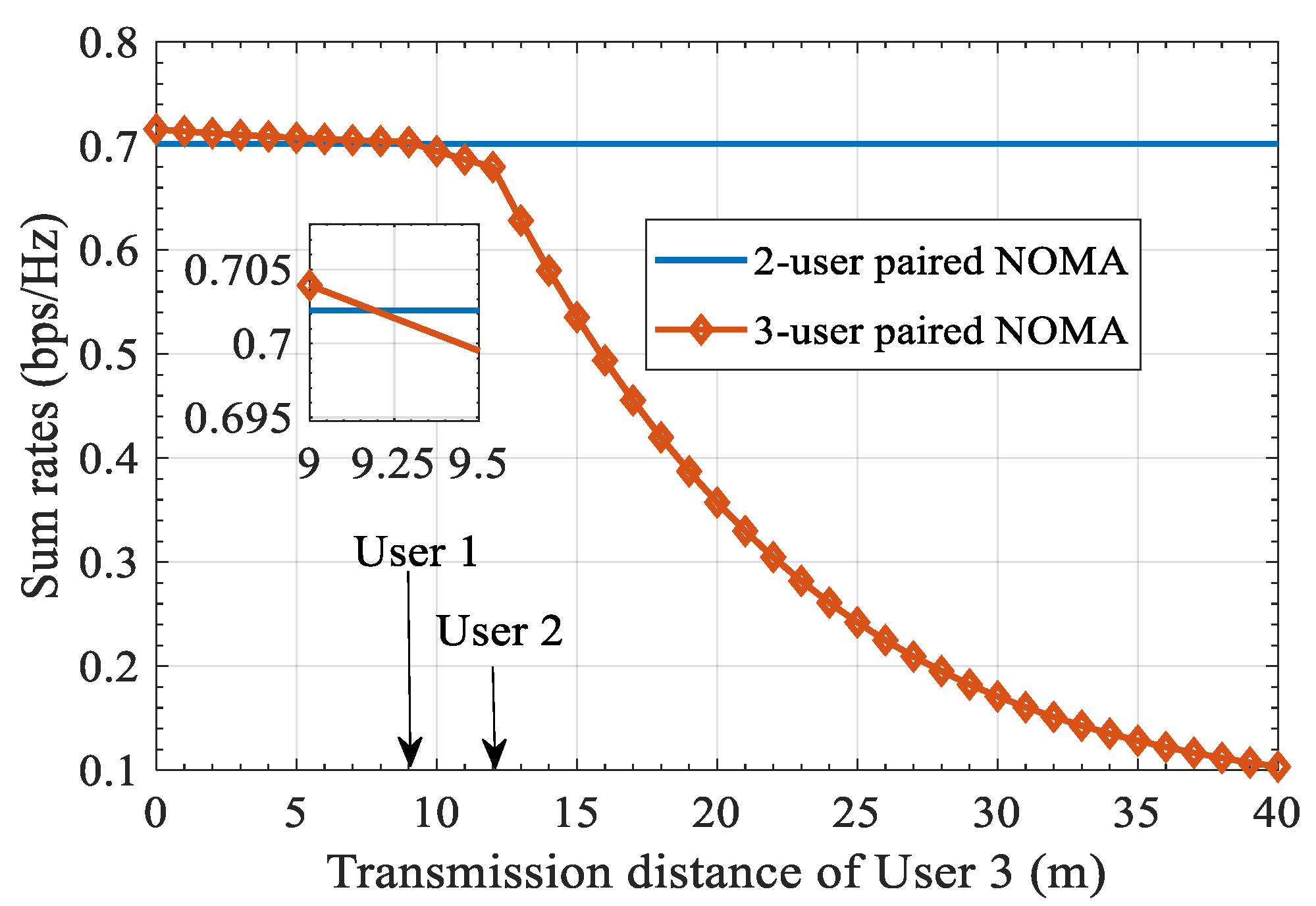
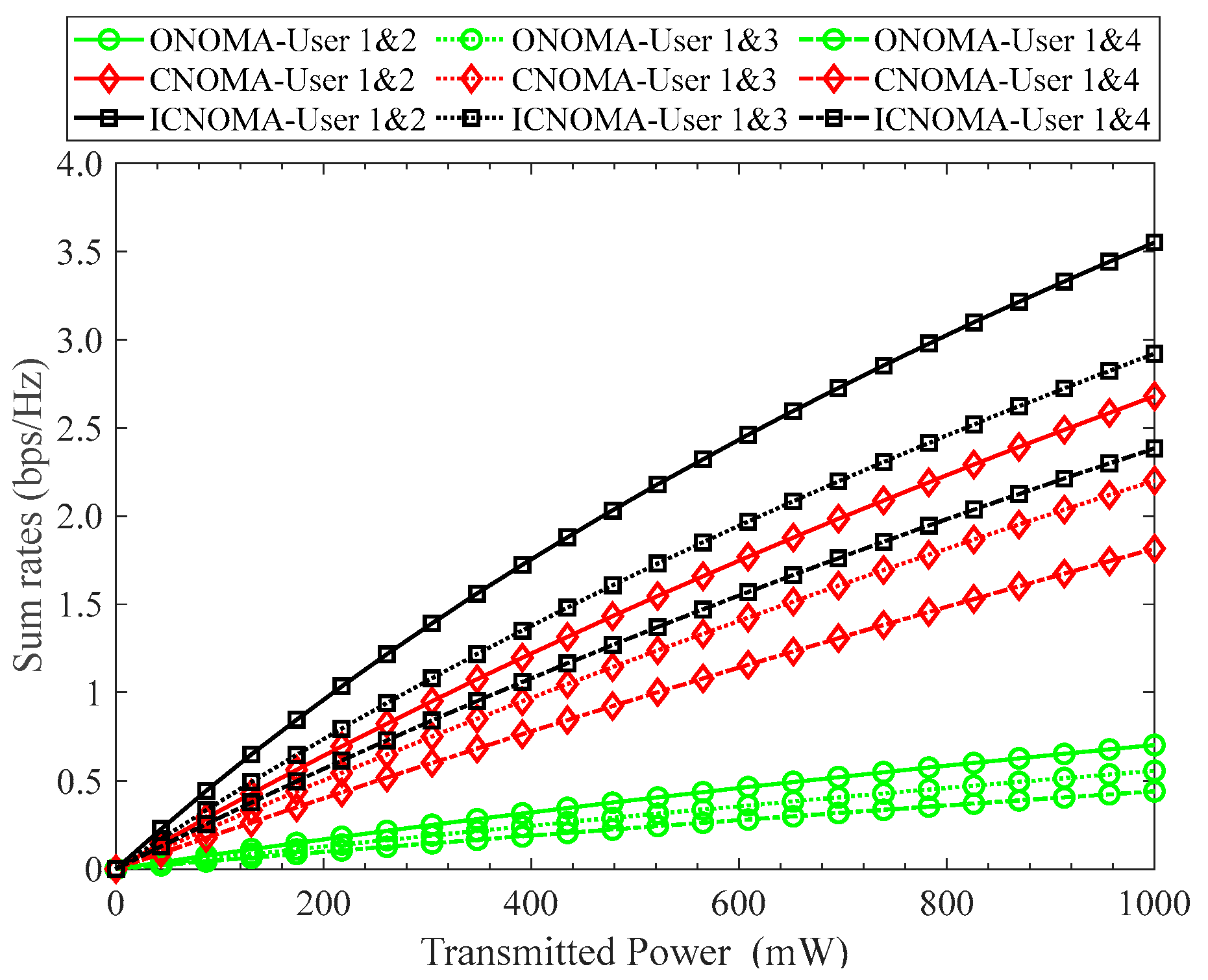
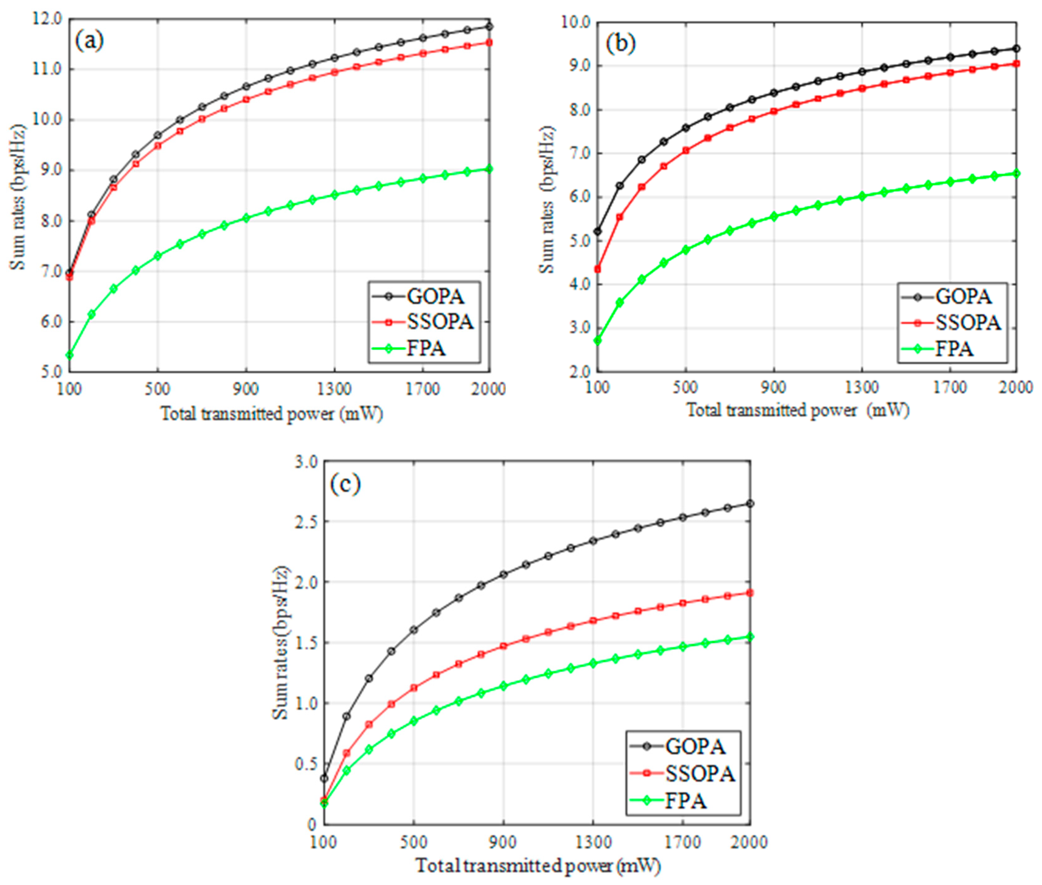
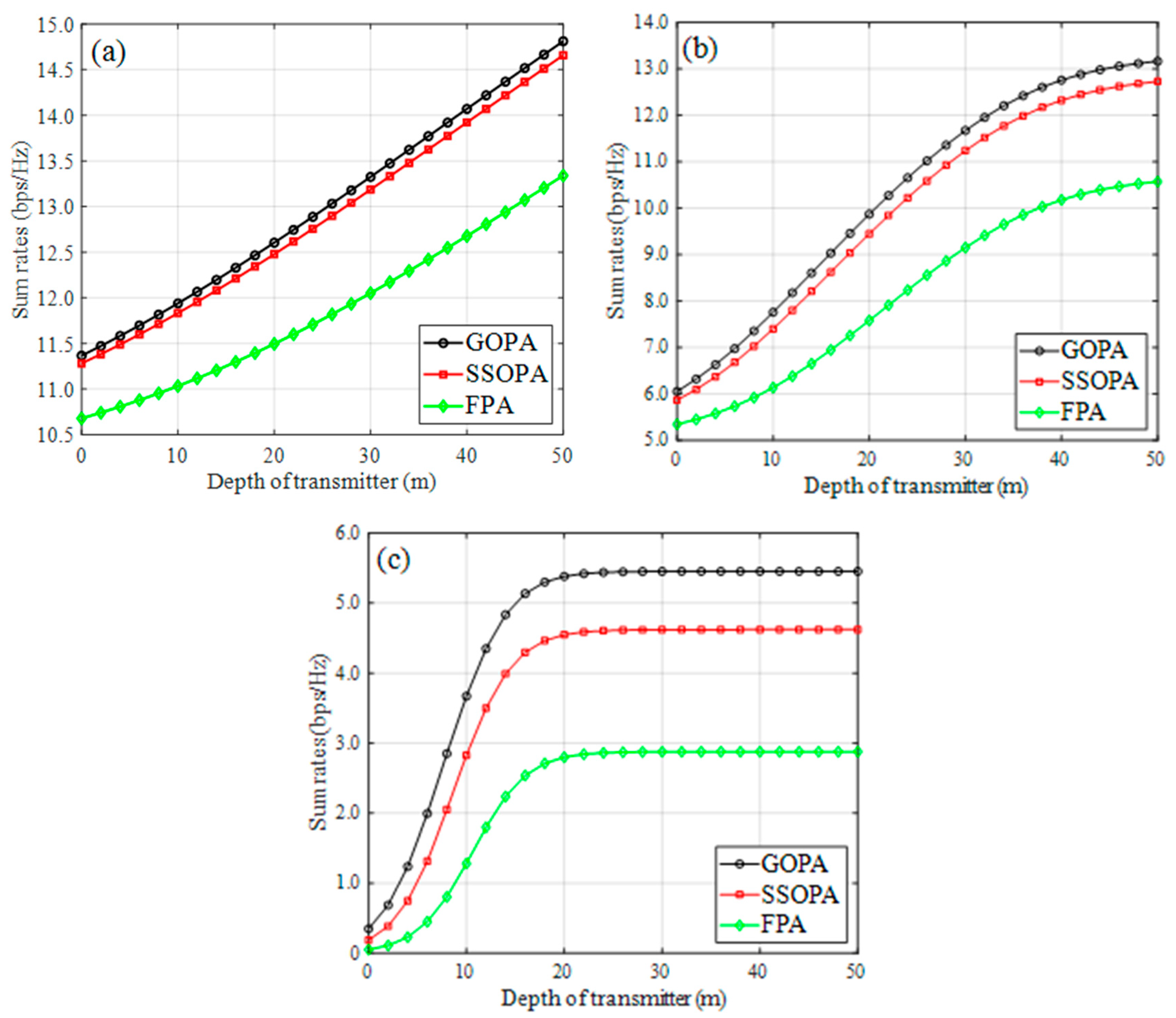
5.2. Performance Evaluations
6. Conclusions
Author Contributions
Funding
Data Availability Statement
Acknowledgments
Conflicts of Interest
References
- Kaushal, H.; Kaddoum, G. Underwater Optical Wireless Communication. IEEE Access 2016, 4, 1518–1547. [Google Scholar] [CrossRef]
- Schirripa Spagnolo, G.; Cozzella, L.; Leccese, F. Underwater Optical Wireless Communications: Overview. Sensors 2020, 20, 2261. [Google Scholar] [CrossRef] [PubMed]
- Xue, K.; Ma, R.; Wang, D.; Shen, M. Optical Classification of the Remote Sensing Reflectance and Its Application in Deriving the Specific Phytoplankton Absorption in Optically Complex Lakes. Remote Sens. 2019, 11, 184. [Google Scholar] [CrossRef]
- Uudeberg, K.; Aavaste, A.; Kõks, K.-L.; Ansper, A.; Uusõue, M.; Kangro, K.; Ansko, I.; Ligi, M.; Toming, K.; Reinart, A. Optical Water Type Guided Approach to Estimate Optical Water Quality Parameters. Remote Sens. 2020, 12, 931. [Google Scholar] [CrossRef]
- Verniers, K.; Nobby, S. Impact of LED Optical Bandwidth Limitation on the Performance of Power Switched Signaling. In Proceedings of the 2020 12th International Symposium on Communication Systems, Networks and Digital Signal Processing (CSNDSP), Porto, Portugal, 20–22 July 2020; pp. 1–6. [Google Scholar]
- Elouafadi, R.; Raiss El Fenni, M.; Benjillali, M. NOMA Clustering for Improved Multicast IoT Schemes. J. Sens. Act. Netw. 2022, 11, 26. [Google Scholar] [CrossRef]
- Islam, S.M.R.; Avazov, N.; Dobre, O.A.; Kwak, K.-S. Power-Domain Non-Orthogonal Multiple Access (NOMA) in 5G Systems: Potentials and Challenges. IEEE Commun. Surv. Tutor. 2017, 19, 721–742. [Google Scholar] [CrossRef]
- Lin, B.; Tang, X.; Zhou, Z.; Lin, C.; Ghassemlooy, Z. Experimental demonstration of SCMA for visible light communications. Opt. Commun. 2018, 419, 36–40. [Google Scholar] [CrossRef]
- Jiang, R.; Sun, C.; Tang, X.; Zhang, L.; Wang, H.; Zhang, A. Joint User-Subcarrier Pairing and Power Allocation for Uplink ACO-OFDM-NOMA Underwater Visible Light Communication Systems. J. Lightwave Technol. 2021, 39, 1997–2007. [Google Scholar] [CrossRef]
- Geldard, C.; Thompson, J.; Popoola, W.O. A Study of Non-Orthogonal Multiple Access in Underwater Visible Light Communication Systems. In Proceedings of the 2018 IEEE 87th Vehicular Technology Conference (VTC Spring), Porto, Portugal, 3–6 June 2018; pp. 1–6. [Google Scholar]
- Akhtar, M.W.; Hassan, S.A.; Jung, H. On the Symbol Error Probability of STBC-NOMA with Timing Offsets and Imperfect Successive Interference Cancellation. Electronics 2021, 10, 1386. [Google Scholar] [CrossRef]
- Li, Y.; Yu, Z.; Zhou, H.; Tao, J. To Relay or not to Relay: Open Distance and Optimal Deployment for Linear Underwater Acoustic Networks. IEEE Trans. Commun. 2018, 66, 3797–3808. [Google Scholar] [CrossRef]
- Saeed, N.; Celik, A.; Al-Naffouri, T.Y.; Alouini, M.S. Underwater optical wireless communications, networking, and localization: A survey. Ad Hoc Netw. 2019, 94, 101935. [Google Scholar] [CrossRef]
- Jamali, M.V.; Chizari, A.; Salehi, J.A. Performance Analysis of Multi-Hop Underwater Wireless Optical Communication Systems. IEEE Photonics Technol. Lett. 2017, 29, 462–465. [Google Scholar] [CrossRef]
- Saeed, N.; Celik, A.; Alouini, M.S.; Al-Naffouri, T.Y. Performance Analysis of Connectivity and Localization in Multi-Hop Underwater Optical Wireless Sensor Networks. IEEE. Trans. Mob. Comput. 2019, 18, 2604–2615. [Google Scholar] [CrossRef]
- Inoue, Y.; Kodama, T.; Kimura, T. Global Optimization of Relay Placement for Seafloor Optical Wireless Networks. IEEE Trans. Wirel. Comm. 2021, 20, 1801–1815. [Google Scholar] [CrossRef]
- Xing, F.; Yin, H.; Shen, Z.; Leung, V.C.M. Joint Relay Assignment and Power Allocation for Multiuser Multirelay Networks over Underwater Wireless Optical Channels. IEEE Internet Things J. 2020, 7, 9688–9701. [Google Scholar] [CrossRef]
- Palitharathna, K.W.S.; Suraweera, H.A.; Godaliyadda, R.I.; Herath, V.R.; Thompson, J.S. Average Rate Analysis of Cooperative NOMA Aided Underwater Optical Wireless Systems. IEEE Open J. Comm. Soc. 2021, 2, 2292–2310. [Google Scholar] [CrossRef]
- Palitharathna, K.W.S.; Suraweera, H.A.; Godaliyadda, R.I.; Herath, V.R.; Ding, Z. Impact of Receiver Orientation on Full-Duplex Relay Aided NOMA Underwater Optical Wireless Systems. In Proceedings of the 2020 IEEE International Conference on Communications (ICC), Virtual Conference, 7–11 June 2020; pp. 1–7. [Google Scholar]
- Miroshnikova, N.E.; Petruchin, G.S.; Titovec, P.A. Estimation of the Effect of Dispersion on the Communication Range in a Wireless Underwater Optical Channel. In Proceedings of the 2021 Systems of Signal Synchronization, Generating and Processing in Telecommunications (SYNCHROINFO), Svetlogorsk, Russia, 30 June–2 July 2021; pp. 1–4. [Google Scholar]
- Aravind, J.V.; Kumar, S.; Prince, S. Mathematical Modelling of Underwater Wireless Optical Channel. In Proceedings of the 2018 International Conference on Communication and Signal Processing (ICCSP), Chennai, India, 3–5 April 2018; pp. 776–780. [Google Scholar]
- Sticklus, J.; Hoeher, P.A.; Röttgers, R. Optical Underwater Communication: The Potential of Using Converted Green LEDs in Coastal Waters. IEEE J. Ocean Eng. 2019, 44, 535–547. [Google Scholar] [CrossRef]
- Wang, K.; Gong, C.; Zou, D.; Xu, Z. Turbulence Channel Modeling and Non-Parametric Estimation for Optical Wireless Scattering Communication. J. Lightwave Technol. 2017, 35, 2746–2756. [Google Scholar] [CrossRef]
- Bi, C.; Qing, C.; Wu, P.; Jin, X.; Liu, Q.; Qian, X.; Zhu, W.; Weng, N. Optical Turbulence Profile in Marine Environment with Artificial Neural Network Model. Remote Sens. 2022, 14, 2267. [Google Scholar] [CrossRef]
- Zhang, L.; Wang, Z.; Wei, Z.; Chen, C.; Wei, G.; Fu, H.Y.; Dong, Y. Towards a 20 Gbps multi-user bubble turbulent NOMA UOWC system with green and blue polarization multiplexing. Opt. Express 2020, 28, 31796–31807. [Google Scholar] [CrossRef]
- Zhang, J.; Gao, G.; Wang, B.; Guan, X.; Yin, L.; Chen, J.; Luo, B. Background noise resistant underwater wireless optical communication using Faraday atomic line laser and filter. J. Lightwave Technol. 2021, 40, 63–73. [Google Scholar] [CrossRef]
- Patterson, A.M.; Spence, J.H.; Fischer, R.W. Evaluation of underwater noise from vessels and marine activities. In Proceedings of the IEEE/OES Acoustics in Underwater Geosciences Symposium, Rio de Janeiro, Brazil, 25–27 July 2013; pp. 1–9. [Google Scholar]
- Essiambre, R.-J.; Kramer, G.; Winzer, P.J.; Foschini, G.J.; Goebel, B. Capacity Limits of Optical Fiber Networks. J. Lightwave Technol. 2010, 28, 662–701. [Google Scholar] [CrossRef]
- Balti, E.; Guizani, M.; Hamdaoui, B. Hybrid Rayleigh and Double-Weibull over impaired RF/FSO system with outdated CSI. In Proceedings of the 2017 IEEE International Conference on Communications (ICC), Paris, France, 21–25 May 2017; pp. 1–6. [Google Scholar]
- Benjebbovu, A.; Li, A.; Saito, Y.; Kishiyama, Y.; Harada, A.; Nakamura, T. System-level performance of downlink NOMA for future LTE enhancements. In Proceedings of the 2013 IEEE Globecom Workshops (GC Wkshps), Atlanta, GA, USA, 9–13 December 2013; pp. 66–70. [Google Scholar]
- Zhang, H.; Wang, B.; Chen, C.; Cheng, X.; Li, H. Resource Allocation in UAV-NOMA Communication Systems Based on Proportional Fairness. J. Commun. Inf. Netw. 2020, 5, 111–120. [Google Scholar] [CrossRef]
- Ghosh, J.; Haci, H.; Kumar, N.; Al-Utaibi, K.A.; Sait, S.M.; So-In, C. A Novel Channel Model and Optimal Power Control Schemes for Mobile mmWave Two-Tier Networks. IEEE Access 2022, 10, 54445–54458. [Google Scholar] [CrossRef]
- Gagnon, F.; Dahman, G.; Poitau, G. Extending the ITU-R P.530 Deep-Fading Outage Probability Results to SIMO-MRC and MIMO-MRC Line-of-Sight Systems. IEEE Wirel. Commun. Lett. 2018, 7, 1086–1089. [Google Scholar] [CrossRef]
- Aryan, M.; Alejandro, R. RES: Regularized Stochastic BFGS Algorithm. IEEE Trans. Signal Process. 2014, 62, 6089–6104. [Google Scholar]
- Grubisic, S.; Carpes, W.P.; Bastos, J.P.A.; Santos, G. Association of a PSO Optimizer with a Quasi-3D Ray-Tracing Propagation Model for Mono and Multi-Criterion Antenna Positioning in Indoor Environments. IEEE Trans. Magn. 2013, 49, 1645–1648. [Google Scholar] [CrossRef]
- Tong, Z.; Yang, X.; Chen, X.; Zhang, H.; Zhang, Y.; Zou, H.; Zhao, L.; Xu, J. Quasi-omnidirectional transmitter for underwater wireless optical communication systems using a prismatic array of three high-power blue LED modules. Opt. Express 2021, 29, 20262–20274. [Google Scholar] [CrossRef]
- Elamassie, M.; Bariah, L.; Uysal, M.; Muhaidat, S.; Sofotasios, P.C. Capacity Analysis of NOMA-Enabled Underwater VLC Networks. IEEE Access 2021, 9, 153305–153315. [Google Scholar] [CrossRef]


| Water Type | ɑ (m−1) | b (m−1) | c (m−1) |
|---|---|---|---|
| Pure seawater | 0.053 | 0.003 | 0.056 |
| Clean seawater | 0.114 | 0.037 | 0.151 |
| Coastal seawater | 0.179 | 0.219 | 0.398 |
| Harbor water | 0.295 | 1.875 | 2.170 |
| Algorithm | Time Complexity | Problem Size |
|---|---|---|
| FPA | O(smax) | 107M |
| GOPA | 1570M/τ | |
| SSOPA | O(smax) | 278MK |
| x | Transmitted signal | y | Received signal |
| P | Power | h | Channel gain |
| n | Number of the receiving nodes, n ∈ [1, N] | m | Number of the relay nodes, m ∈ [1, M] |
| a | NOMA power allocation coefficient | Ζ | Power allocation ratio |
| Noise power | smax | Iterations of algorithm | |
| τ | Step-size factor | k | Number of the particle swarm, k ∈ [1, K] |
| δ | Amplification coefficient | d | Transmission distance |
| c | Attenuation coefficient | θ | Beam divergence angle |
| θ0 | Inclination angle | α | Optical fading amplitude |
| Parameters | Values |
|---|---|
| System bandwidth B | 32 MHz |
| Total transmitted power Ptotal | 2000 mW |
| Divergence angle of the transmitter θ0 | 30° |
| Aperture area of the optical receiver Ade | 0.01 m2 |
| P-I modulation conversion coefficient ηtr | 0.9 A/W |
| Responsibility of the photodetector ηde | 0.9 W/A |
| Relay Selection | Relay Selection | Rtotal (bps/Hz) | ||
|---|---|---|---|---|
| Scenario 1 | GOPA | C1 (i = 1, j = 4) | C2(i = 2, j = 3) | 7.92 |
| SSOPA | C1 (i = 1, j = 4) | C2(i = 2, j = 3) | 7.62 | |
| FPA | C2 (i = 1, j = 3) | C2(i = 2, j = 4) | 6.10 | |
| Scenario 2 | GOPA | C1 (i = 1, j = 4) | C2(i = 2, j = 3) | 11.05 |
| SSOPA | C1 (i = 1, j = 4) | C2(i = 2, j = 3) | 10.87 | |
| FPA | C1 (i = 1, j = 3) | C2(i = 2, j = 4) | 8.65 | |
| Scenario 3 | GOPA | C1 (i = 1, j = 4) | C1 (i = 2, j = 3) | 2.15 |
| SSOPA | C1 (i = 1, j = 4) | C1 (i = 2, j = 3) | 1.50 | |
| FPA | C1 (i = 1, j = 3) | C1 (i = 2, j = 4) | 0.37 |
| Relay Selection | Pm (mW) | Rtotal (bps/Hz) | ||||
|---|---|---|---|---|---|---|
| GOPA | C1 (i = 1, j = 4) | 421.52 | 578.48 | 0.206 | 0.796 | 7.92 |
| C2 (i = 2, j = 3) | 361.20 | 638.80 | 0.377 | 0.623 | ||
| SSOPA | C1 (i = 1, j = 4) | 445.73 | 554.27 | 0.211 | 0.789 | 7.62 |
| C2 (i = 2, j = 3) | 356.85 | 643.15 | 0.384 | 0.616 | ||
| FPA | C1 (i = 1, j = 4) | 500.00 | 500.00 | 0.191 | 0.809 | 6.10 |
| C2 (i = 2, j = 3) | 500.00 | 500.00 | 0.401 | 0.599 | ||
| N-relay with GOPA | (i = 1, j = 4) | 1000.00 | 0.00 | 0.051 | 0.949 | 1.08 |
| (i = 2, j = 3) | 1000.00 | 0.00 | 0.113 | 0.887 | ||
| N-relay with SSOPA | (i = 1, j = 4) | 1000.00 | 0.00 | 0.045 | 0.955 | 0.97 |
| (i = 2, j = 3) | 1000.00 | 0.00 | 0.101 | 0.899 | ||
| N-relay with FPA | (i = 1, j = 4) | 1000.00 | 0.00 | 0.034 | 0.966 | 0.74 |
| (i = 2, j = 3) | 1000.00 | 0.00 | 0.087 | 0.913 |
Publisher’s Note: MDPI stays neutral with regard to jurisdictional claims in published maps and institutional affiliations. |
© 2022 by the authors. Licensee MDPI, Basel, Switzerland. This article is an open access article distributed under the terms and conditions of the Creative Commons Attribution (CC BY) license (https://creativecommons.org/licenses/by/4.0/).
Share and Cite
Liang, Y.; Yin, H.; Jing, L.; Ji, X.; Wang, J. Performance Analysis of Relay-Aided NOMA Optical Wireless Communication System in Underwater Turbulence Environment. Remote Sens. 2022, 14, 3894. https://doi.org/10.3390/rs14163894
Liang Y, Yin H, Jing L, Ji X, Wang J. Performance Analysis of Relay-Aided NOMA Optical Wireless Communication System in Underwater Turbulence Environment. Remote Sensing. 2022; 14(16):3894. https://doi.org/10.3390/rs14163894
Chicago/Turabian StyleLiang, Yanjun, Hongxi Yin, Lianyou Jing, Xiuyang Ji, and Jianying Wang. 2022. "Performance Analysis of Relay-Aided NOMA Optical Wireless Communication System in Underwater Turbulence Environment" Remote Sensing 14, no. 16: 3894. https://doi.org/10.3390/rs14163894