Automatic Detection of Pothole Distress in Asphalt Pavement Using Improved Convolutional Neural Networks

Abstract

To realize the intelligent and accurate measurement of pavement surface potholes, an improved You Only Look Once version three (YOLOv3) object detection model combining data augmentation and structure optimization is proposed in this study. First, color adjustment was used to enhance the image contrast, and data augmentation was performed through geometric transformation. Pothole categories were subdivided into P1 and P2 on the basis of whether or not there was water. Then, the Residual Network (ResNet101) and complete IoU (CIoU) loss were used to optimize the structure of the YOLOv3 model, and the K-Means++ algorithm was used to cluster and modify the multiscale anchor sizes. Lastly, the robustness of the proposed model was assessed by generating adversarial examples. Experimental results demonstrated that the proposed model was significantly improved compared with the original YOLOv3 model; the detection mean average precision (mAP) was 89.3%, and the F1-score was 86.5%. On the attacked testing dataset, the overall mAP value reached 81.2% (−8.1%), which shows that this proposed model performed well on samples after random occlusion and adding noise interference, proving good robustness.

1. Introduction

Pavement surface distresses including potholes pose a significant threat to driving safety. Therefore, rapid detection and intelligent maintenance of potholes are prerequisites for pavement management [1]. However, conventional pothole detection mainly relies on manual methods [2], which suffer from strong subjectivity, high cost, a long cycle, and which are not conducive to rapid detection. The emergence of digital image processing technology (DIP) makes the digital detection of pavement potholes possible, which is a method of processing images through denoising, enhancing, restoring, segmenting, and extracting features using a computer, including edge detection [3], threshold segmentation [4], and morphological processing [5]. These methods are widely used in pavement distress detection.

Although DIP has made good progress in pothole detection [6], it cannot achieve the automatic detection of potholes accurately. Fortunately, with the progress of deep learning (DL) [7], especially the emergence of convolutional neural networks (CNNs) in 2012 [8], DL models represented by CNNs have gradually shown their superiority in object detection because they can quickly and accurately detect objects by automatically extracting features [9]. Subsequently, CNNs have been extensively used in remote sensing [10], the healthcare industry [11], and other fields [12,13]. Furthermore, they are also applied in scenarios such as transportation infrastructure [14,15], pedestrian detection [16], unmanned driving [17], and pavement distress detection [18]. At present, there are two kinds of object detection algorithms in identifying pavement distress: one-stage algorithms and two-stage algorithms.

On the one hand, two-stage algorithms first generate the proposal region, and then perform CNN-based classification and identification of the region. Representatives include the region-based CNN (R-CNN) series [19], R-FCN [20], and SPP-Net [21]. Nie et al. [22] applied the faster R-CNN model to detect pavement distress; these experimental results represented a significant breakthrough, but the dataset used was small. Then, Pei et al. [23] further refined the faster R-CNN model by modifying the anchor size and combining it with the VGG-16 network based on the expanded dataset, whose final detection accuracy was 89.97%. Song et al. [24] further considered the distress conditions for different pavements and proposed a method based on the faster R-CNN model to identify various distresses accurately. In conclusion, these studies failed to achieve rapid detection because the two-stage algorithm has numerous network parameters, which makes the period of training and testing time-consuming.

On the other hand, the emergence of one-stage object detection models addressed the issues of low efficiency in the two-stage models. One-stage algorithms directly set sizes of the multiscale anchor, integrating classification and regression into one step instead of region proposal, which improves the model’s speed. Cao et al. [25] proposed a single-shot multi-box detector-based (SSD) object detection method on airport pavement with high detection accuracy (89.3%). However, the sizes of anchors in the SSD model were manually determined by data distribution, and a method for automatic anchor generation was urgently requested. The emergence of You Only Look Once version three (YOLOv3) solves this problem [26]. As one of the classic one-stage object detection models, YOLOv3 adopts the K-Means algorithm to generate anchors of three scales, which can realize multiscale detection. Zhu et al. [27] used the YOLOv3 model to detect pavement distress, and they verified the feasibility of YOLOv3 by comparing it with several mainstream object detection models. YOLOv3 has a high comprehensive performance, but the detection accuracy is not good enough to meet the maintenance needs.

Many studies have improved the detection performance of the YOLOv3 model, and the existing improvement methods mainly include data augmentation, network structure adjustment, improvement of the loss function, and hyperparameter optimization [28]. Liu et al. [29] expanded the number of samples in the dataset through data augmentation to avoid overfitting, which improved the generalization ability of the YOLOv3 model. Bochkovskiy et al. [30] combined the SPP-Net and PANet networks to replace the original FPN network in YOLOv3, enabling the network to fully extract small object features. Tang et al. [31] employed the distance between the anchor and the cluster center point to define the loss function, which was more reasonable for evaluating the loss of the model. However, the above studies were aimed at cracks, and this approach has rarely been applied to potholes. In addition, the enhancement methods are not comprehensive enough, lacking the consideration of the actual scene. Meanwhile, the robustness of the model has not been evaluated.

Therefore, a method of combining data augmentation and YOLOv3 structure optimization is proposed to study pavement pothole detection. The main contributions of this study are as follows:

(1)

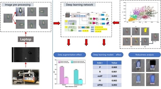
The pothole dataset was contrast-enhanced by color adjustment, and geometric transformation was adopted to expand the number of samples. A data augmentation strategy suitable for potholes was proposed to train DL models.

(2)

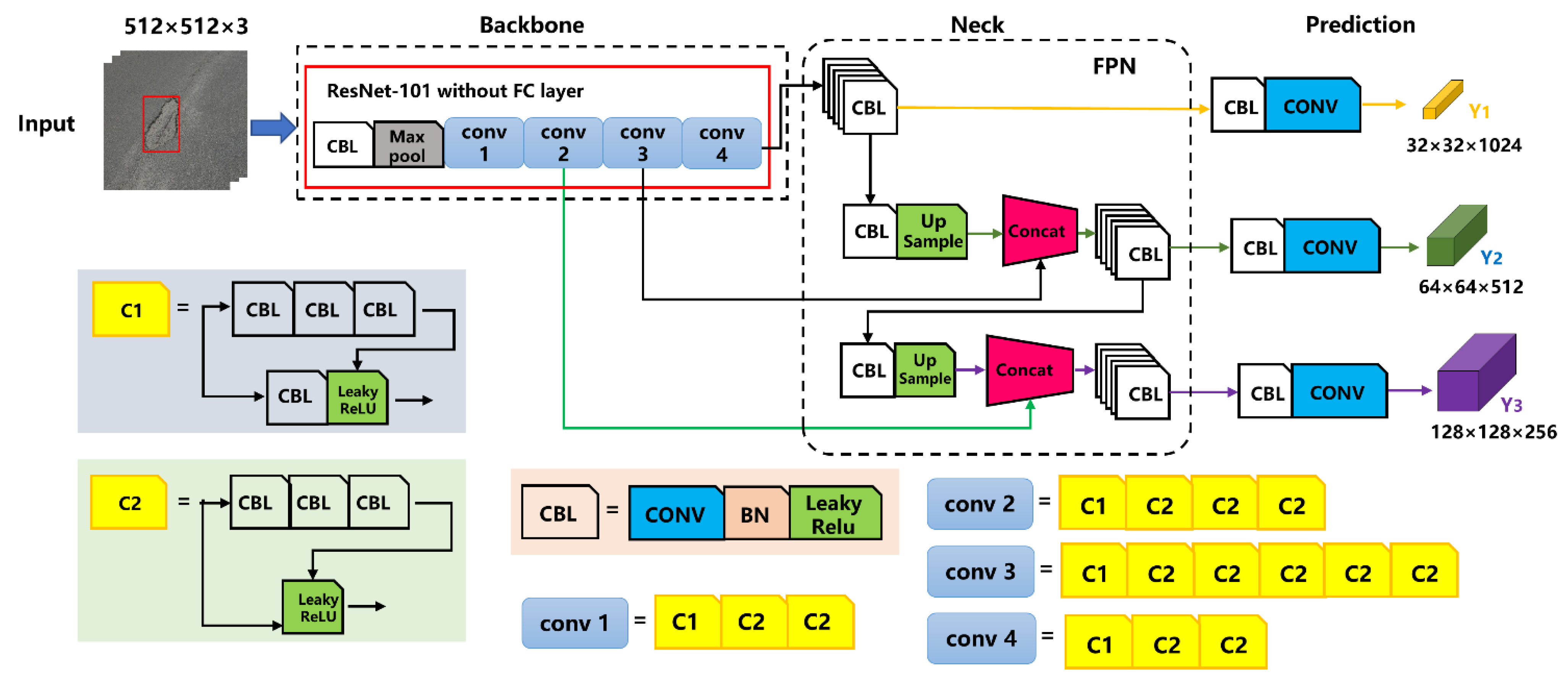
The ResNet101 network was used to improve the feature extraction network of YOLOv3. Complete intersection over union (CIoU) was applied to measure the loss of the proposed model. The anchor sizes were modified by the K-Means++ algorithm. An object detection model applicable for potholes was established.

(3)

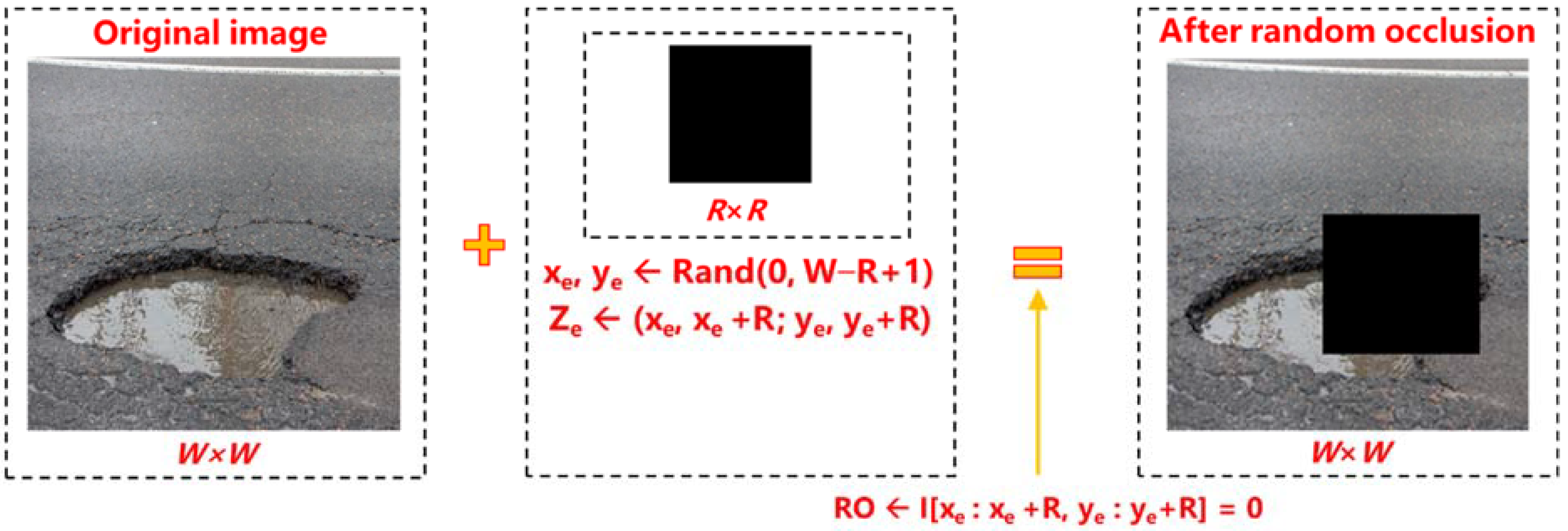
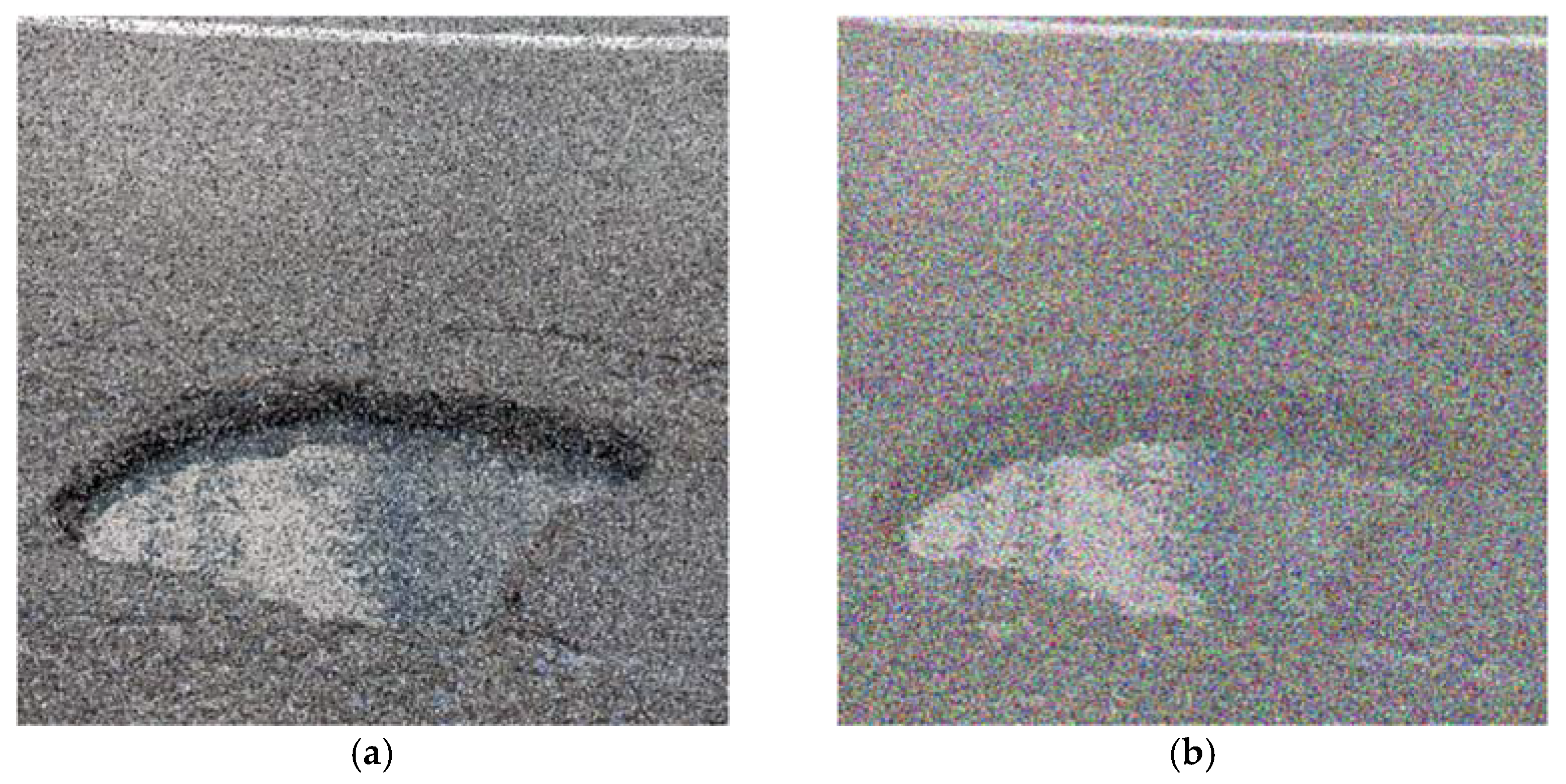
Adversarial samples of potholes were generated by random occlusion and adding noise before testing, which verified the robustness of this model.

The remainder of this study is organized as follows: the methodology is described in Section 2, including the image preprocessing methods, YOLOv3 network structure, robustness analysis, and evaluation index. The experimental results and analysis are presented in Section 3. Conclusions are drawn in Section 4.

2. Methodology

2.1. Pavement Pothole Dataset

The pavement distress images were collected from typical provincial highways in Zhejiang Province. The dataset was captured using a mobile mapping system using an onboard high-definition camera (HD camera), as illustrated in Figure 1. Figure 1 illustrates the acquisition process of gray images and local details of camera (the front and the back). The detection field of the camera takes the maximum detection width of the single lane as 3750 mm. If two cameras are selected, the lateral visual field of one camera must be at least 2000 mm. Two cameras were selected here, and the camera’s information is listed in

Table 1. Technical parameters of the high-definition camera.

Camera Features	Details	Camera Features	Details
Type	Basler raL2048-80km	Power supply requirements (typical value)	3 W
Interface	Camera Link	Type of light-sensitive chips	CMOS
Resolution ratio	3854 px × 2065 px	Size of light-sensitive chips	14.3 mm

. Camerlink interface meets the demand of high-speed image acquisition, and it has the advantages of strong anti-interference ability and low power consumption. CMOS cameras are more suitable for high-speed acquisition with low cost and low power consumption. One obtained image is shown on the right of Figure 1.

The original gray image was 3854 by 2065 pixels. A total of 500 pavement images were collected. After the filtration, 300 images were used for model training, and 100 images were chosen for testing. Two color adjustment methods were used to improve the image brightness. Then, four types of geometric transformation were performed on the preprocessed images. Considering the small scale of the dataset, the risk of information leakage [32], and the low accuracy of model performance, the dataset was divided into a training dataset, validation dataset, and testing dataset according to the ratio of 6:2:2 [33]. Details are shown in

Table 2. Detailed division information of image dataset of pavement potholes.

Dataset	Training Dataset	Validation Dataset	Testing Dataset
Image with potholes	480	160	160
Image without potholes	720	240	240
Total	1200	400	400

.

Potholes on rainy days accumulate water, while potholes on sunny days are mostly dry. Therefore, the potholes with accumulated water and dry surfaces were marked as P1 and P2, respectively. All labeling work was performed using LabelImg software (v1.8.6) [34].

2.2. Pothole Data Pre-Processing

To adjust the brightness of the dataset, two types of color adjustment method were used. The contrast and sharpness of the image were modified. The performance of DL models depends on the size and the quality of the dataset. Therefore, data augmentation was used to address the above issues [35]. Four geometric augmentation methods were adopted [36]. Details are described below.

2.2.1. Color Adjustment

The pavement pothole images were three-channel color images. Each color pixel featured the three components of red, green, and blue, referring to the color image at a specific spatial position and, thus, forming a vector to describe the image. For the processing of color images, two color augmentation operations (contrast and sharpness) were used [37].

To solve the problem of low contrast caused by the small gray-level range of the pothole image, contrast augmentation was used to enlarge the gray-level range of the pothole image and make the image clearer [38]. Using the hue–saturation–intensity (HSI) color model, the probability smoothing method was conducted for the components of intensity and saturation, which converted the intensity and saturation components into a uniform distribution. The calculation formulas of the intensity and the saturation components are shown in Equation (1) and Equation (2), respectively.

$$y_{1k}=F(x_{1k})=P\left\{x_I\le x_{Ik}\right\}={\displaystyle {\sum }_{m=0}^{k}f(x_{Im})={\displaystyle {\sum }_{m=0}^{k}P\left\{x_I\le x_{Ik}\right\}}},$$

(1)

$$y_{st}=F(\left.x_{1k}\right|x_{Ik})={\displaystyle {\sum }_{m=0}^{t}f(\left.x_{Sm}\right|x_{Ik})={\displaystyle {\sum }_{m=0}^t\frac{P\left\{x_I=x_{Ik},x_s=x_{Sm}\right\}}{P\left\{x_I=x_{Ik}\right\}}}},$$

(2)

where k = 0, 1, …, L − 1 and t = 0, 1, …, M − 1; L and M represent discrete levels of intensity and saturation, respectively. X = (x_H, x_S, x_I)^T is a vector of color pixels representing each image. F(∙) is a probability function, and F(Z) = F(x_I, x_S) = P{x_I ≤ x_I, x_S ≤ x_S}.

Sharpness eliminates the blurring of the pothole image by increasing the contrast of the pixels in the neighborhood, making the pothole object clearer. Laplace sharpness adds gradient values (Laplace operator) to the pothole image [39]. The enhancement method based on the Laplace operator is shown in Equation (3).

$$g(x,y)=f(x,y)-\left[\begin{array}{c}{\nabla }^{2}R(x,y)\\ {\nabla }^{2}G(x,y)\\ {\nabla }^{2}B(x,y)\end{array}\right],$$

(3)

where g(x, y) is the pothole image after sharpness, f(x, y) is original pothole image, and ▽²R(x, y), ▽²G(x, y), and▽²B(x, y) are the Laplace operators of each component (red, green, and blue) of the color images, respectively.

2.2.2. Geometric Transformation

As a traditional data augmentation method, geometric transformation was performed on images through specific operations such as rotation, flipping, and cropping. The shape of the pothole target was mainly polygonal, with randomness in all directions. Four operations of rotating 90° clockwise, 180°, 90° anticlockwise, and random crop were used on the basis of the above features.

The rotation of pothole images refers to forming a new image by rotating the central point of an image at a certain angle as a reference point, which can effectively expand the amount of data.

The random crop method could produce a better effect on learning the main features of potholes while increasing model stability, which was realized by randomly cropping the corner of the image. Specifically, it was assumed that the main feature of potholes (P) is F, and the collected image contains background noise (B). That is, the pothole’s main feature in the captured image is defined as C, which is expressed as (F, B). It is expected to learn F, but possible to learn (F, B), thus resulting in overfitting. Potholes are generally in the middle of the image. Their main features (F) are highly unlikely to be cut, while B is the contrary. This is equivalent to the weight distribution of the two during training. Considering the extreme case (that is, when the weight allocation is only 0 or 1), the information gain of F is large, and the learner is more likely to learn F while ignoring B, as shown in Equation (4). X_c represents several cases of learning feature information in extreme cases. For example, X_c⁽¹⁾ = (1·F, 0·B) is the case when F weighs 1, while B is 0.

$$X_c^{(1)}=(1\cdot F,0\cdot B),X_c^{(2)}=(1\cdot F,1\cdot B),X_c^{(3)}=(0\cdot F,1\cdot B),\dots$$

(4)

The two color adjustment methods and four data augmentation methods are listed in

Table 3. Examples of data augmentation of pavement potholes.

Pre-Processing Steps	Original Image	Color Transformation (Contrast Adjustment)		Geometric Transformation (Data Augmentation)
		Contrast	Sharpness	Rotating 90° Anticlockwise	Rotating 90° Clockwise	Rotating 180°	Random Crop
Potholes with water
Potholes without water

, illustrated with examples.

2.3. Object Detection

2.3.1. YOLOv3–ResNet101 Structure

YOLOv3 is a state-of-the-art object detection algorithm with fast speed and high accuracy. An end-to-end training and prediction method is adopted in YOLOv3, which is applicable for practical engineering applications [26]. In this paper, YOLOv3 was used as the basic framework for pothole detection. The ResNet101 network [40] was used instead of the traditional DarkNet-53 network as the feature extraction network. The proposed network structure is illustrated in Figure 2.

First, the pothole image was passed through a ResNet101 network without a fully connected layer to perform feature extraction. Then, upsampling and tensor concatenating were performed on the feature map. Thus, outputs at three different scales (Y1, Y2, Y3), as illustrated in Figure 2, were obtained. The multiscale method was employed to detect pothole objects of various sizes. The created detector had well-balanced performance regardless of the pothole sizes.

For a stacked layer, x is the input, and H(x) is the learned feature. Thus, what is learned in the residual network is the residual F(x) = H(x) − x, while the original learned feature is H(x) = F(x) + x. This way of learning makes it easier to learn from raw features compared to the direct way. When F(x) = 0, the stacking layer performs identity mapping, and the performance of this network does not degrade. As a residual network, the ResNet18 network [40] can extract deeper-level features, thus having a more accurate understanding of the image. However, the ResNet18 has more network parameters than the deep residual network, resulting in a large number of training calculations. To decrease the computational cost, ResNet101 employs a bottleneck design structure. It has a convolution of inputs 7 × 7 × 64, then goes through 33 (3 + 4 + 23 + 3) building blocks, each of which has three layers, and finally an FC layer (for classification), for a total of 1 + 33 × 3 + 1 = 101 layers. Subsequently, five feature maps of different sizes, C1, C2, C3, C4, and C5, were generated. They were different in size, and each pixel on the feature map had a different receptive field, corresponding to the original image, which was equivalent to dividing the original image into grids of different sizes. The ResNet101 network was selected. Figure 3 shows the improvement process.

To avoid gradient disappearance and speed up model convergence, ResNet101 adopts batch normalization (BN) [41]. BN converts the input distribution into a standard normal distribution with a mean of 0 and a variance of 1.

In addition, the detailed network parameters of YOLOv3–ResNet101 are given in

Table 4. Network parameters of YOLOv3–ResNet101.

Network	Layer Name	Output Size	Parameters
ResNet101	conv1	512 × 512 × 3	conv, 7 × 7 × 64, stride 2
	conv2	256 × 256 × 64	>max pool, 3 × 3, stride 2 bottleneck: 1 × 1 $\left[\begin{array}{c}1\times 1\times 64\\ 3\times 3\times 64\\ 1\times 1\times 256\end{array}\right]\times 3$
	conv3	128 × 128 × 256	bottleneck: 1 × 1 $\left[\begin{array}{c}1\times 1\times 128\\ 3\times 3\times 128\\ 1\times 1\times 512\end{array}\right]\times 4$
	conv4	64 × 64 × 512	bottleneck: 1 × 1 $\left[\begin{array}{c}1\times 1\times 256\\ 3\times 3\times 256\\ 1\times 1\times 1024\end{array}\right]\times 23$
	conv5	32 × 32 × 1024	bottleneck: 1 × 1 $\left[\begin{array}{c}1\times 1\times 512\\ 3\times 3\times 512\\ 1\times 1\times 2048\end{array}\right]\times 3$
YOLOv3	Y1	32 × 32 × 1024	3 anchors $\left[\begin{array}{c}3\times 3\times 1024\\ 1\times 1\times 1024\end{array}\right]\times 2$
	Y2	64 × 64 × 512	3 anchors $\left[\begin{array}{c}3\times 3\times 1024\\ 1\times 1\times 1024\end{array}\right]\times 2$
	Y3	128 × 128 × 256	3 anchors $\left[\begin{array}{c}3\times 3\times 1024\\ 1\times 1\times 1024\end{array}\right]\times 2$

.

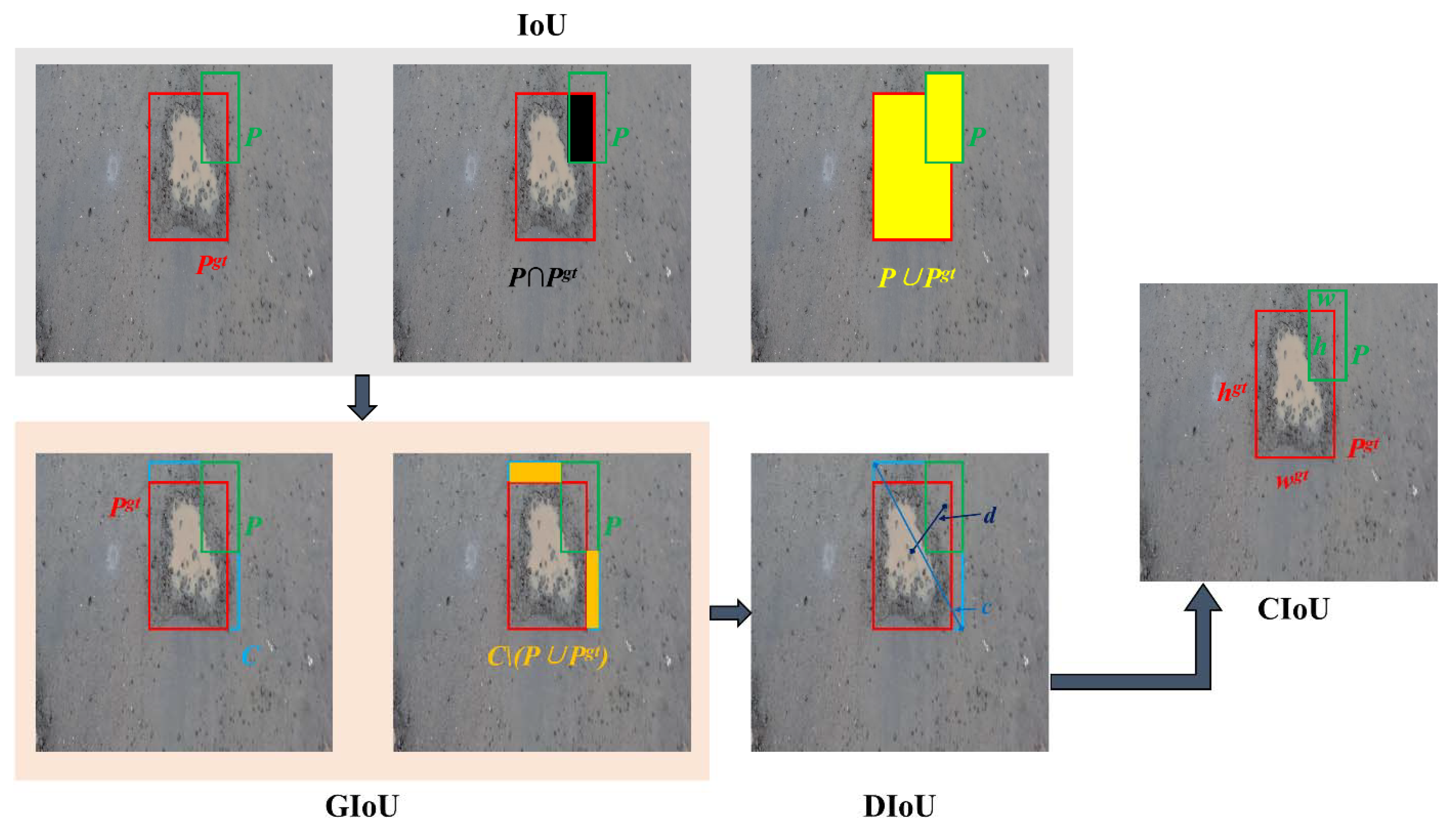
2.3.2. Loss Function

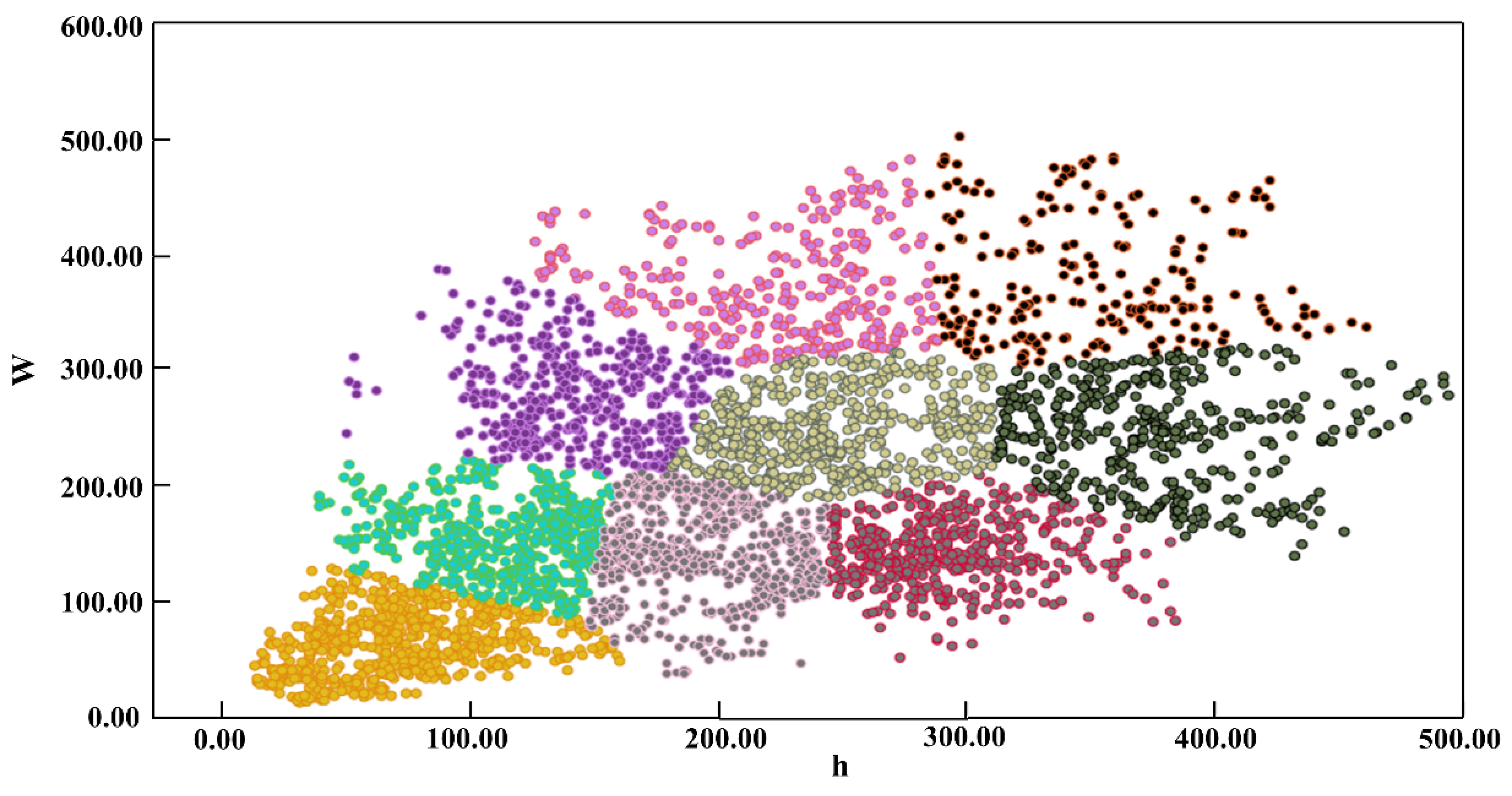
The loss function of YOLOv3 consists of category loss, confidence loss, and position loss. The calculation formula is shown in Equation (5).

$$Loss=Los{s}_{class}+Los{s}_{conf}+Los{s}_{loc}.$$

(5)

Figure 4 shows the calculations of intersection over union (IoU) and other loss functions [42], where P represents the prediction box, P^gt represents the ground truth, and IoU is defined as the ratio of intersection and union between P, P^gt, which reflects the degree of overlap between the two. However, there are two problems with this calculation: first, when the prediction box is not overlapped with the real box, the IoU is 0, and the gradient return cannot be carried out; second, the calculation result is only related to the overlap area and cannot measure the way of intersection between two boxes. Therefore, the IoU is not a comprehensive and accurate measure of the degree of overlap.

As a result, improvements to IoU have constantly been proposed. Generalized intersection over union (GIoU) considers the nonoverlapping regions; however, it is scale-invariant and is not conducive to multiscale pothole detection. The distance between P and P^gt is directly minimized to speed up convergence in distance IoU (DIoU); nevertheless, the aspect ratio of the two is not considered.

Complete IoU (CIoU) was selected as the loss function in this paper. Three important geometric factors of bounding-box regression loss are taken into account in CIoU: overlap area, center point distance, and aspect ratio, which allows a more stable and accurate convergence. The CIoU is calculated as shown in Equation (6).

$$\left\{\begin{array}{c}Los{s}_{CIoU}=1-IoU+\frac{{\rho }^2(P,P^{gt})}{c^2}\\ v=\frac{4}{{\pi }^2}{(\arctan \frac{w^{gt}}{h^{gt}}-\arctan \frac{w}{h})}^2\\ \alpha =\frac{v}{(1-IoU)+v}\end{array}\right.,$$

(6)

where v represents the consistency of the pothole’s aspect ratio, a is the positive tradeoff parameter, w^gt and h^gt are the width and length of P^gt, respectively, and w and h are the width and length of P, respectively.

2.3.3. Anchor Size

An anchor is mainly used to solve the issue that the scale and aspect ratio vary too much in object detection. Through the anchor mechanism, the multiscale and aspect ratio are divided into several subspaces to reduce the difficulty of pothole detection, making the model easier to learn. In the original YOLOv3 structure, the scale and aspect ratio of the anchor are determined using the COCO dataset. However, the application object of the dataset is the pavement pothole; thus, the original anchor size is not suitable for the research scene of this paper. There is an urgent need to perform anchor clustering on the pothole dataset. The K-Means algorithm needs to determine the initial cluster center manually [26]; thus, the K-Means++ was used to cluster the real annotation boxes more accurately. The K-Means++ algorithm firstly selected a random point from the dataset as the center point and calculated the distance between the sample and each known center point. Then, M points were found far from the known center point. Lastly, a random point from M samples was chosen as the center. The clustering results were more concentrated, and the aspect ratio was more in line with the characteristics of the pothole dataset. The results are illustrated in Figure 5, and the size distribution of the anchor is shown in

Table 5. Multiscale anchor size of potholes based on K-Means++.

Detection Scale	Anchor Size
Scale 1: 32 × 32	(176, 312)	(335, 247)	(285, 362)
Scale 2: 64 × 64	(126, 236)	(285.5, 132)	(213, 201)
Scale 3: 128 × 128	(34, 35)	(72, 79)	(149, 126)

. The obtained anchor sizes were employed to replace the original parameters for training and testing, which reduced the difficulty of model training.

2.3.4. Robustness Verification

There are many shielding objects around potholes in actual scenes, such as leaves, road repair, and moving vehicles. Meanwhile, the same pothole can present different characteristics under different lighting conditions due to changes over time. Therefore, it is necessary to verify the proposed model’s robustness in such a complex background. The existing analysis methods on robustness are mainly divided into traditional methods and adversarial attacks because of the different research fields and research angles [43]. The traditional method involves applying this model to another scene for verification and evaluating its robustness through the testing results. Adversarial attacks make the model produce false results by continuously adding tiny perturbations (adversarial examples) to the image.

Given the above problems, and considering that the potholes were interfered by shielding objects, the random occlusion (RO) method [44] was adopted to set the pixel value in a square area of the input image to zero. Details of random occlusion are shown in Figure 6, where x_e, y_e are random coefficients, and Z_e is the random occlusion area. The pixel color in the random occlusion area was set to zero.

Salt-and-pepper noise [45] and Gaussian noise [46] were also added to simulate the noise problem during the acquisition process. Figure 7 shows the noise-attacked image, in which the ratio of salt-and-pepper noise was 0.10, and the mean value and variance of Gaussian noise were 0 and 0.1, respectively. The noise had a great effect on the pothole.

2.3.5. Evaluation Index

To evaluate the accuracy and performance of the object detection model, precision (P), recall rate (R), mean average precision (mAP), and F1-score were selected. TP represents that the potholes are detected correctly when there exist potholes. FP represents that a pothole is detected when there is no pothole. FN represents that no pothole is detected when there exist potholes. TN represents that no pothole is detected when there is no pothole. The detailed calculation formulas are described in Equations (7)–(10).

$$P=\frac{TP}{TP+FP}.$$

(7)

$$R=\frac{TP}{TP+FN}.$$

(8)

$$mAP=\frac{{({\displaystyle {\int }_0^{1}P(r)dR})}_{P1}+{({\displaystyle {\int }_0^{1}P(r)dR})}_{P2}}{2}.$$

(9)

$$F1=\frac{2\times P\times R}{P+R}.$$

(10)

Furthermore, the calibration error index (ECE) [47] was selected to demonstrate the improved overfitting results after the data augmentation strategy. The calculation formula of the ECE index is described as follows [48]:

$$ECE={\displaystyle \sum _{b=1}^5\frac{n_b}{N}}\left|A(b)-confidence(b)\right|.$$

(11)

The confidence interval [0, 1] was divided into five bins, where the detection results of each pothole image were saved. In Equation (11), b represents the b-th bin, and n_b refers to the number of samples in the b-th bin. N is the sum of samples. A(b) is the average value of the ground truth of the samples in the b-th bin. Moreover, confidence(b) represents the average value of the model’s predicted probabilities in the b-th bin. A smaller difference between A(b) and confidence(b) indicates a higher model confidence.

3. Results and Discussion

The effect of the data augmentation on the detection result was studied by comparing the detection effect of the object detection models on the testing set before and after augmentation. To evaluate the proposed model from the perspectives of accuracy and performance, two control groups (the original YOLOv3 model and the YOLOv3–ResNet101 model with the new backbone) and the experimental group (YOLOv3–ResNet101 model with modified anchors) were set. Furthermore, several mainstream object detection models were also used to detect the pothole dataset in this study, including faster R-CNN, Cascade R-CNN, and SSD.

Model training and testing were conducted on a Windows 10 system using Python 3.7. The CPU was an Intel (R) Core (TM) i7-7700 CPU. The model reached convergence after 100 epochs. Detailed training parameters are presented in

Table 6. Values of the training parameters.

Hyperparameters	Value
Batch size	2
Epochs	100
Learning rate	0.00125
Weight decay	L2
Optimizer	Momentum
Momentum	0.9

.

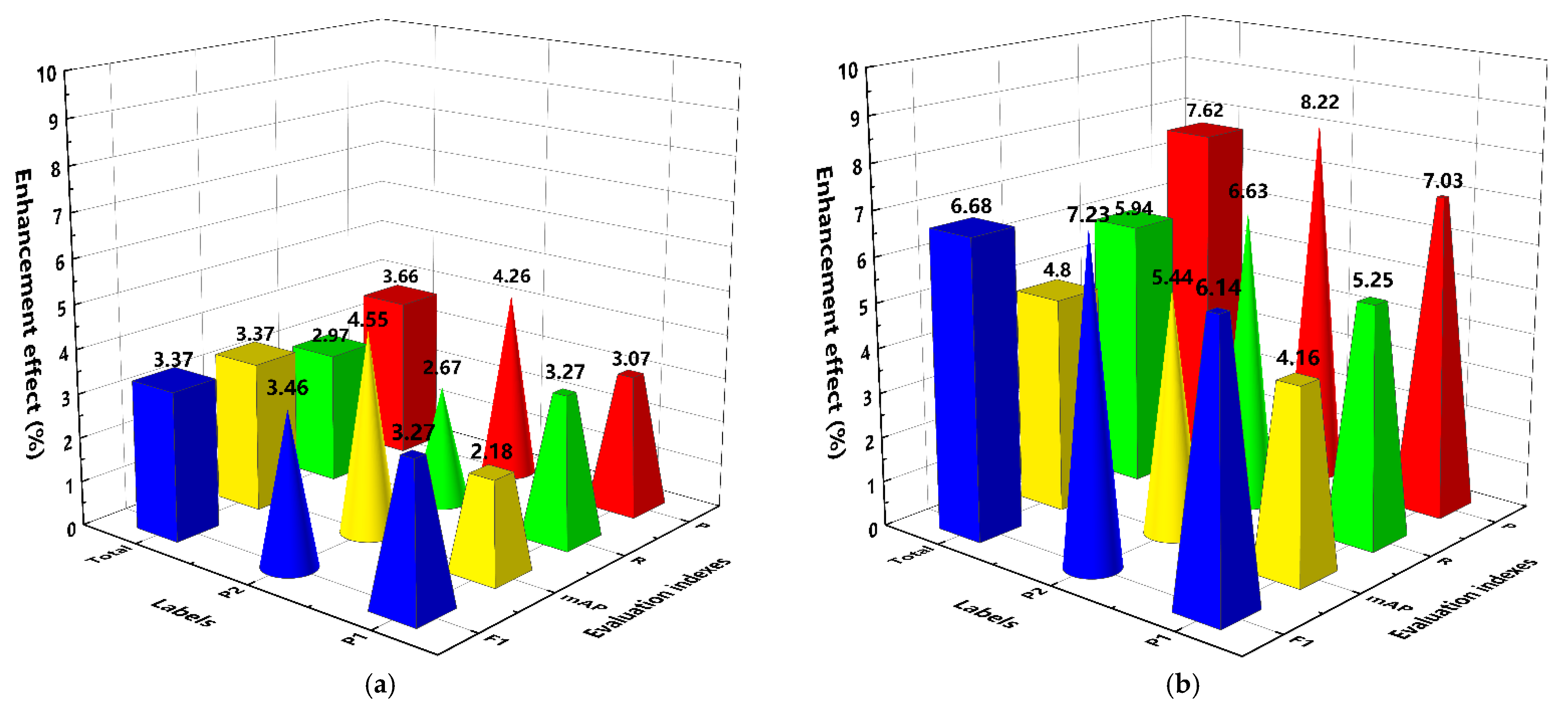
3.1. Results of Data Augmentation

Evaluation indices of the YOLOv3 model and proposed model before and after data augmentation are listed in

Table 7. Evaluation index results of YOLOv3 model and proposed model before and after data augmentation.

Evaluation Indices	P			R			mAP			F1
	P1	P2	Total	P1	P2	Total	P1	P2	Total	P1	P2	Total
YOLOv3	0.734	0.677	0.705	0.742	0.693	0.718	0.749	0.704	0.727	0.737	0.685	0.711
YOLOv3 (aug)	0.764	0.720	0.742	0.775	0.720	0.747	0.771	0.749	0.760	0.769	0.720	0.744
Proposed model	0.802	0.784	0.793	0.830	0.773	0.801	0.853	0.838	0.845	0.816	0.780	0.798
Proposed model (aug)	0.872	0.866	0.869	0.882	0.840	0.861	0.895	0.892	0.893	0.877	0.852	0.865

, where “(aug)” denotes the detection result obtained by the augmented dataset. It can be seen that the P value, R value, mAP, and F1 score of the two object detection models were improved after data augmentation, with a ratio of 2–9%. Data augmentation expanded the number of samples, increased the diversities of labels, ensured the relative balance between the two labels (P1 and P2), and reduced the probability of misidentification. Therefore, the proposed augmentation method could effectively improve the detection effect of the object detection model.

Data augmentation had different effects on different models. Figure 8 shows the enhancement effects of the two models. For the original YOLOv3 model, the improvement degree of the P value, R value, mAP, and F1 score was 2–5%, and the mAP of P2 had the highest improvement of 4.55%. Similarly, for the proposed model, the improvement degree of all evaluation indices was 4–9%, and the P value of P2 had the highest increasement of 8.22%. Generally, the proposed model had a more significant improvement effect on the evaluation indicators based on the enhanced dataset.

Figure 9 shows the effect of calibrating the model using the ECE index. ECE values of the YOLOv3 model and the proposed model decreased significantly after data augmentation, by 62.8% and 69.6%, respectively. The ECE value of the proposed model dropped to 0.088 (a very small value), which shows that the data augmentation strategy is effective in promoting the confidence of the model and improving the overfitting problem.

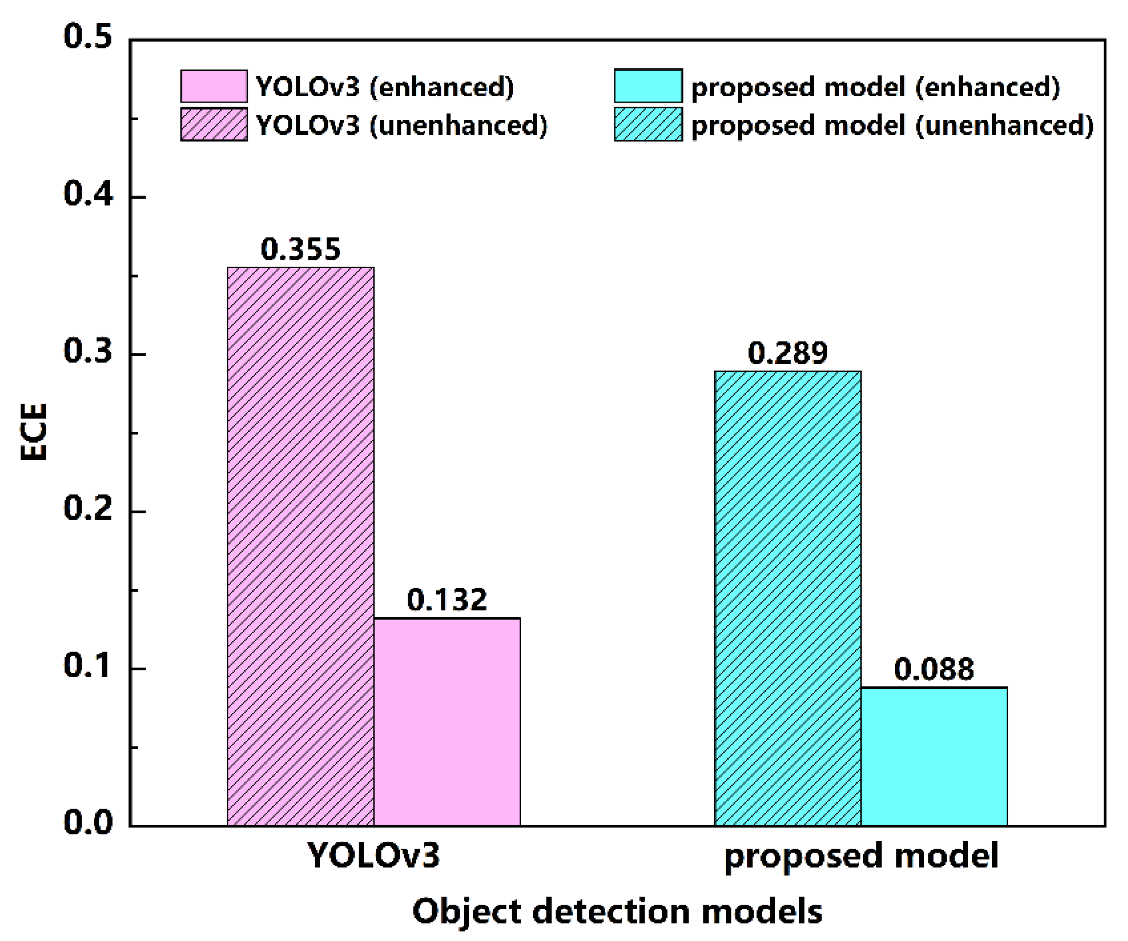
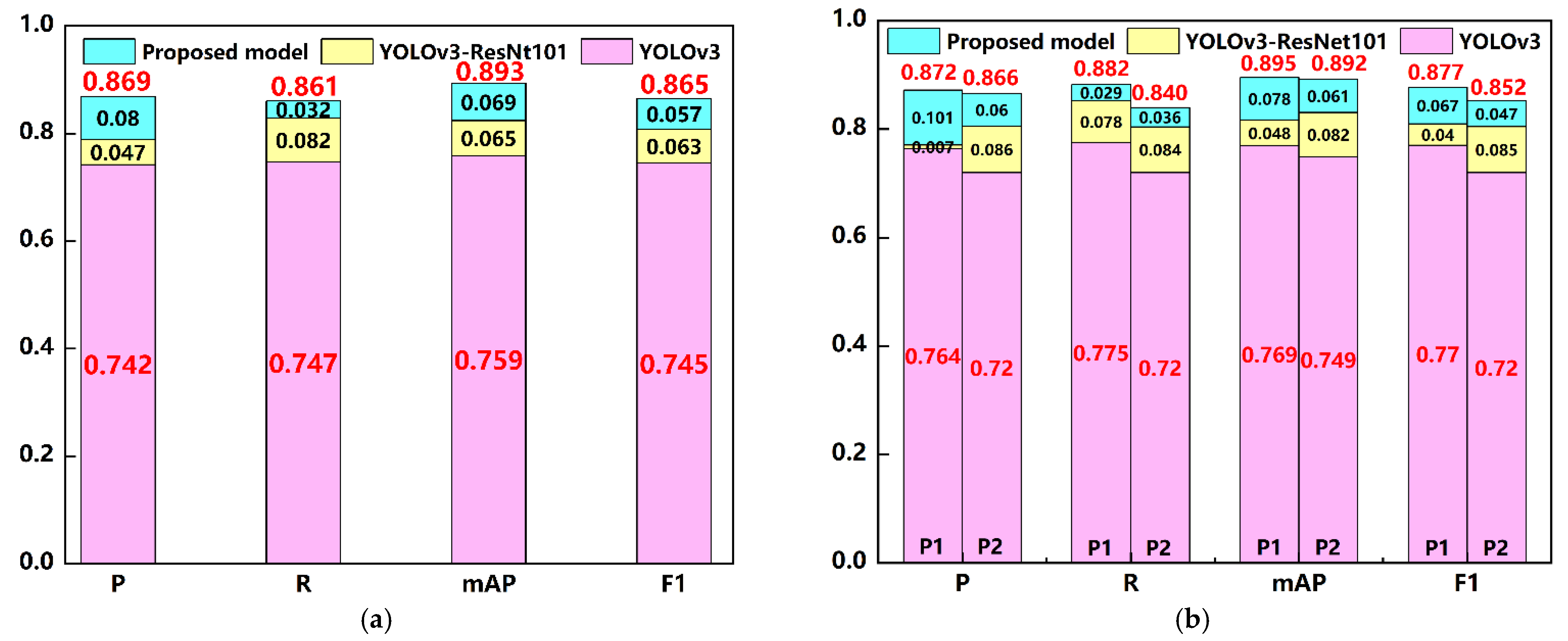
3.2. Evaluation of Different DL Models

The performance of the improved model’s detection effect is shown in Figure 10.

As shown in Figure 10a, YOLOv3–ResNet101 had a significant improvement in all indices compared with the original YOLOv3. Specifically, the mAP and F1 score increased by 6.5% and 6.3%, respectively. The improvement of the P value was 4.7%, which demonstrates that the YOLOv3–ResNet101 model showed a better effect on pothole detection. It was verified that the proposed ResNet101 network was effective, allowing a deeper understanding of the deeper semantic information of the potholes. Furthermore, the proposed model had a greater improvement. The mAP and F1 score were increased by 6.9% and 5.7% compared to the YOLOv3–ResNet101 model, highlighting the great contribution of the modified anchor sizes to the detection performance.

Moreover, Figure 10b shows the detection effects of the YOLOv3 model and the improved model on P1 and P2, respectively. The indices of P1 and P2 labels were all improved in the YOLOv3–ResNet101 model; this improvement was further enlarged in the proposed model. In the original YOLOv3 model, the four indices of P1 were higher than those of P2 because the potholes with water showed different colored surfaces inside and outside the damaged area, making them easier to detect. As for YOLOv3–ResNet101, the differences between the four indices of P1 and P2 were narrowed. Furthermore, this phenomenon was obvious in the proposed model. In terms of mAP values, P2 was fairly close to P1. This indicates that the modified strategies in this study had a greater improvement in P2 than P1.

In addition, the detection results of different object detection models are listed in

Table 8. Comparison of detection results of different object detection models for potholes.

Evaluation Indices		Faster R-CNN [49]	Cascade R-CNN [50]	SSD [51]	YOLOv3–DarkNet53 [26]	YOLOv3–ResNet101	Proposed Model
P	P1	0.807	0.800	0.747	0.764	0.771	0.872
	P2	0.817	0.804	0.751	0.720	0.806	0.866
	Total	0.812	0.802	0.749	0.742	0.789	0.869
R	P1	0.793	0.794	0.733	0.775	0.853	0.882
	P2	0.822	0.810	0.738	0.720	0.804	0.840
	Total	0.807	0.802	0.736	0.747	0.829	0.861
mAP	P1	0.825	0.797	0.798	0.769	0.817	0.895
	P2	0.814	0.805	0.751	0.749	0.831	0.892
	Total	0.819	0.801	0.775	0.759	0.824	0.893
F1	P1	0.798	0.831	0.742	0.770	0.810	0.877
	P2	0.800	0.803	0.744	0.720	0.805	0.852
	Total	0.799	0.817	0.743	0.745	0.808	0.865
AP50		0.819	0.801	0.775	0.759	0.824	0.893
AP75		0.744	0.763	0.685	0.625	0.750	0.841
AP90		0.782	0.783	0.730	0.692	0.784	0.867

. It can be seen that the faster R-CNN model and cascade R-CNN model performed well in various indices because of their advantages, and the accuracy remained nearly above 80%. The accuracy of the SSD model and the original YOLOv3 model was slightly lower than that of the two-stage algorithms, which was caused by sacrificing accuracy for faster training and detection. The improvement effect of the proposed model was obvious; the overall P value, F1 score, and mAP value reached 86.9%, 86.5%, and 89.3%, respectively, which were higher than those of the two-stage methods, realizing the accurate detection of potholes. The rationality and feasibility of our modified strategies were proven in the proposed model.

To verify the localization accuracy of the proposed model, the detection results of faster R-CNN, cascade R-CNN, SSD, YOLOv3–Darknet53, YOLOv3–Resnet101, and the proposed model were compared. AP values with different IoU thresholds (0.50, 0.75, and 0.90) were calculated, and the results are shown in Table 8. It can be seen that the localization accuracy of the proposed model was higher that of the faster R-CNN model, with a significance difference of 7.4% between the two models. The localization accuracy of the original YOLOv3 model was 6.0% lower than that of faster R-CNN. The proposed model could effectively improve the localization accuracy of pothole detection.

3.3. Robustness Analysis

Table 9. Detection indexes of the attacked testing dataset.

Evaluation Indices	IoU50			IoU75			IoU90
	P1	P2	Total	P1	P2	Total	P1	P2	Total
P	0.788	0.793	0.790	0.733	0.738	0.736	0.275	0.277	0.276
R	0.763	0.802	0.783	0.718	0.746	0.732	0.266	0.248	0.257
mAP	0.810	0.814	0.812	0.764	0.773	0.769	0.211	0.325	0.268
F1	0.775	0.797	0.786	0.737	0.743	0.740	0.240	0.238	0.239

lists the evaluation indices on the attacked testing dataset. It can be seen that, when the IoU threshold was 0.5, the overall mAP value reached 0.812, which decreased by 9.98% compared with that before attack. To more intuitively compare the performance of the proposed model on the attacked testing dataset,

Table 10. Examples of detection results of the attacked pothole images.

Labels	Original Images	Proposed Model	Proposed Model (Random Occlusion)	Proposed Model (Salt-and-Pepper Noise Attacked)	Proposed Model (Gaussian Noise Attacked)
P1 (pothole with water)
P2 (pothole without water)

describes four detection examples of typical pothole distress.

As shown in the table, the accuracy of the proposed model on the adversarial attack samples decreased because the random occlusion layer and the added noise destroyed the semantic information around the potholes, which hindered identification of the object. Random occlusion had great influence on the detection results. When ~50% occlusion (50% occlusion is similar to car occlusion) was set, the occluded pothole area could be correctly detected. However, in P2 (pothole without water), the occluded area was incorrectly detected as a pothole, which reduced the overall accuracy. Salt-and-pepper noise brought great damage to pothole targets, and P1 in two pictures was even wrongly detected as P2, which may be because salt-and-pepper noise destroyed the semantic characteristics of water on the surface, making it difficult to detect the existence of water. Gaussian noise was less destructive than salt-and-pepper noise, but the detection accuracy also decreased. Generally, the degree of influence of the three perturbation methods on the detection effect was as follows in this experiment: salt-and-pepper noise > random occlusion > Gaussian noise. Noise destruction is difficult to avoid in the process of image acquisition; therefore, it is of great necessity to study a reasonable image denoising method.

3.4. Generalization Performance Analysis

Generalization performance analysis was conducted.

Table 11. Detection examples of the open-source dataset using the proposed model.

Original image
Detection results of the proposed model

describes the typical detection examples on a publicly available dataset [52]. The detection effect of the proposed model on the publicly available dataset was generally good. Although the detection effect was worse than that for the constructed dataset in this paper, the degree of reduction was small. It can be seen from Table 11 that the detection accuracy of the P2 label was higher, but there was a phenomenon of misdetection (row 2 and column 3 of Table 11). It was easy for the proposed model to misidentify manhole covers as P1 labels (row 2 and column 4 in Table 11), which indicated that the proposed model does not have strong detection ability for manhole covers and is not suitable for areas with many manhole covers. Additionally, the proposed model misidentified large pools of water in the public dataset as P1 labels.

4. Conclusions

A modified YOLOv3 model was proposed to detect potholes on the pavement surface under wet and dry conditions in this study. Through data augmentation, modified anchor sizes, improved feature network, and loss function, a model with higher accuracy was proposed, and its robustness was verified. The main conclusions can be drawn as follows:

(1)

An effective image preprocessing strategy for improving and expanding the pothole dataset was proposed using the methods of color adjustment and geometric transformation, which ensured the detection stability of the proposed model.

(2)

The potholes were further subdivided according to whether there was water. The detection results could preliminarily judge the surface state of the pothole and weather conditions.

(3)

The ResNet101 network was adopted to extract features in the YOLOv3 model, which obtained abundant information on potholes. The modified anchor sizes based on the K-Means++ method were more in line with the shapes and sizes of the pothole, which improved the accuracy of the identification and location. The loss function defined by CIoU was of great help for accurate pothole detection.

(4)

The robustness of the proposed model was verified by generating adversarial attack samples through random occlusion and adding noise. Results showed that the overall robustness was good. Specifically, the proposed model was more robust to Gaussian noise under the interference intensity.

It should be noted that perturbations were added to our pothole testing dataset during robustness verification. Multiple methods of perturbation, such as other types of noise and occlusion ratio, need to be evaluated in the future. Despite the limited perturbation methods, the proposed model could provide a reference for pothole detection in the actual scene.

References

1. Liu, S.; Tu, X.; Xu, C.; Chen, L.; Lin, S.; Li, R. An Optimized Deep Neural Network for Overhead Contact System Recognition from LiDAR Point Clouds. Remote Sens. 2021, 13, 4110. [Google Scholar] [CrossRef]
2. Liu, Z.; Gu, X.; Wu, C.; Ren, H.; Zhou, Z.; Tang, S. Studies on the validity of strain sensors for pavement monitoring: A case study for a fiber Bragg grating sensor and resistive sensor. Constr. Build. Mater. 2022, 321, 126085. [Google Scholar] [CrossRef]
3. Luo, Q.; Ge, B.; Tian, Q. A fast adaptive crack detection algorithm based on a double-edge extraction operator of FSM. Constr. Build. Mater. 2019, 204, 244–254. [Google Scholar] [CrossRef]
4. Chen, Y.; Liang, J.; Gu, X.; Zhang, Q.; Deng, H.; Li, S. An improved minimal path selection approach with new strategies for pavement crack segmentation. Measurement 2021, 184, 109877. [Google Scholar] [CrossRef]
5. Liang, J.; Gu, X.; Chen, Y. Fast and robust pavement crack distress segmentation utilizing steerable filtering and local order energy. Constr. Build. Mater. 2020, 262, 120084. [Google Scholar] [CrossRef]
6. Wang, L.; Gu, X.; Liu, Z.; Wu, W.; Wang, D. Automatic detection of asphalt pavement thickness: A method combining GPR images and improved Canny algorithm. Measurement 2022, 196, 111248. [Google Scholar] [CrossRef]
7. Liu, Z.; Chen, Y.; Gu, X.; Yeoh, J.K.; Zhang, Q. Visibility classification and influencing-factors analysis of airport: A deep learning approach. Atmos. Environ. 2022, 278, 119085. [Google Scholar] [CrossRef]
8. Krizhevsky, A.; Sutskever, I.; Hinton, G.E. Imagenet classification with deep convolutional neural networks. Commun. ACM 2017, 60, 84–90. [Google Scholar] [CrossRef]
9. Cha, Y.-J.; Choi, W.; Büyüköztürk, O. Deep Learning-Based Crack Damage Detection Using Convolutional Neural Networks. Comput. Aided Civ. Infrastruct. Eng. 2017, 32, 361–378. [Google Scholar] [CrossRef]
10. Xiong, Y.; Zhou, Y.; Wang, F.; Wang, S.; Wang, Z.; Ji, J.; Wang, J.; Zou, W.; You, D.; Qin, G. A Novel Intelligent Method Based on the Gaussian Heatmap Sampling Technique and Convolutional Neural Network for Landslide Susceptibility Mapping. Remote Sens. 2022, 14, 2866. [Google Scholar] [CrossRef]
11. Puttagunta, M.; Ravi, S. Medical image analysis based on deep learning approach. Multimedia Tools Appl. 2021, 80, 24365–24398. [Google Scholar] [CrossRef] [PubMed]
12. Liu, Z.; Wu, W.; Gu, X.; Li, S.; Wang, L.; Zhang, T. Application of Combining YOLO Models and 3D GPR Images in Road Detection and Maintenance. Remote Sens. 2021, 13, 1081. [Google Scholar] [CrossRef]
13. Xu, J.; Zhang, J.; Sun, W. Recognition of the Typical Distress in Concrete Pavement Based on GPR and 1D-CNN. Remote Sens. 2021, 13, 2375. [Google Scholar] [CrossRef]
14. Deng, T.; Zhou, Z.; Fang, F.; Wang, L. Research on Improved YOLOv3 Traffic Sign Detection Method. Comput. Eng. Appl. 2020, 56, 28–35. [Google Scholar]
15. Liu, Z.; Gu, X.; Dong, Q.; Tu, S.; Li, S. 3D Visualization of Airport Pavement Quality Based on BIM and WebGL Integration. J. Transp. Eng. Part B Pavements 2021, 147, 04021024. [Google Scholar] [CrossRef]
16. Zhou, W.N.; Sun, L.H. A Real-time Detection Method for Multi-scale Pedestrians in Complex Environment. J. Electron. Inf. Technol. 2021, 43, 2063–2070. [Google Scholar]
17. Liu, T.; Wang, Y.; Niu, X.; Chang, L.; Zhang, T.; Liu, J. LiDAR Odometry by Deep Learning-Based Feature Points with Two-Step Pose Estimation. Remote Sens. 2022, 14, 2764. [Google Scholar] [CrossRef]
18. Miao, P.; Srimahachota, T. Cost-effective system for detection and quantification of concrete surface cracks by combination of convolutional neural network and image processing techniques. Constr. Build. Mater. 2021, 293, 123549. [Google Scholar] [CrossRef]
19. Girshick, R.; Donahue, J.; Darrell, T.; Malik, J. Rich Feature Hierarchies for Accurate Object Detection and Semantic Segmentation. In Proceedings of the IEEE Conference on Computer Vision and Pattern Recognition, Columbus, OH, USA, 23–28 June 2014; pp. 580–587. [Google Scholar] [CrossRef]
20. Dai, J.; Li, Y.; He, K.; Sun, J. R-fcn: Object detection via region-based fully convolutional networks. In Proceedings of the Advances in Neural Information Processing Systems 29 (NIPS 2016), Barcelona, Spain, 5–10 December 2016. [Google Scholar]
21. He, K.; Zhang, X.; Ren, S.; Sun, J. Spatial Pyramid Pooling in Deep Convolutional Networks for Visual Recognition. IEEE Trans. Pattern Anal. Mach. Intell. 2015, 37, 1904–1916. [Google Scholar] [CrossRef]
22. Nie, M.; Wang, K. Pavement Distress Detection Based on Transfer Learning. In Proceedings of the 2018 5th International Conference on Systems and Informatics (ICSAI), Nanjing, China, 10–12 November 2018; pp. 435–439. [Google Scholar]
23. Pei, L.; Shi, L.; Sun, Z.; Li, W.; Gao, Y.; Chen, Y. Detecting potholes in asphalt pavement under small-sample conditions based on improved faster region-based convolution neural networks. Can. J. Civ. Eng. 2022, 49, 265–273. [Google Scholar] [CrossRef]
24. Song, L.; Wang, X. Faster region convolutional neural network for automated pavement distress detection. Road Mater. Pavement Des. 2021, 22, 23–41. [Google Scholar] [CrossRef]
25. Cao, X.G.; Gu, Y.F.; Bai, X.Z. Detecting of foreign object debris on airfield pavement using convolution neural network. In Proceedings of the LIDAR Imaging Detection and Target Recognition 2017, Changchun, China, 23–25 July 2017. [Google Scholar]
26. Redmon, J.; Farhadi, A. YOLOv3: An Incremental Improvement. arXiv 2018, arXiv:1804.02767. [Google Scholar]
27. Zhu, J.; Zhong, J.; Ma, T.; Huang, X.; Zhang, W.; Zhou, Y. Pavement distress detection using convolutional neural networks with images captured via UAV. Autom. Constr. 2022, 133, 103991. [Google Scholar] [CrossRef]
28. Liu, Z.; Gu, X.; Yang, H.; Wang, L.; Chen, Y.; Wang, D. Novel YOLOv3 Model With Structure and Hyperparameter Optimization for Detection of Pavement Concealed Cracks in GPR Images. IEEE Trans. Intell. Transp. Syst. 2022, 1–11. [Google Scholar] [CrossRef]
29. Liu, Z.; Yuan, L.; Zhu, M.; Ma, S.; Chen, L. YOLOv3 Traffic sign Detection based on SPP and Improved FPN. Comput. Eng. Appl. 2021, 57, 164–170. [Google Scholar]
30. Bochkovskiy, A.; Wang, C.-Y.; Liao, H.-Y.M. YOLOv4: Optimal Speed and Accuracy of Object Detection. arXiv 2020, arXiv:2004.10934. [Google Scholar]
31. Tan, Y.; Cai, R.; Li, J.; Chen, P.; Wang, M. Automatic detection of sewer defects based on improved you only look once algorithm. Autom. Constr. 2021, 131, 103912. [Google Scholar] [CrossRef]
32. Cao, Y.; Zhou, Y. Multi-Channel Fusion Leakage Detection. J. Cyber Secur. 2020, 5, 40–52. [Google Scholar]
33. Guo, T.W.; Lu, K.; Chai, X.; Zhong, Y. Wool and Cashmere Images Identification Based on Deep Learning. In Proceedings of the Textile Bioengi-neering and Informatics Symposium (TBIS), Manchester, UK, 25–28 July 2018; pp. 950–956. [Google Scholar]
34. Tzutalin. LabelImg. Git Code. 2015. Available online: https://github.com/tzutalin/labelImg (accessed on 5 October 2015).
35. Xue, J.; Xu, H.; Yang, H.; Wang, B.; Wu, P.; Choi, J.; Cai, L.; Wu, Y. Multi-Feature Enhanced Building Change Detection Based on Semantic Information Guidance. Remote Sens. 2021, 13, 4171. [Google Scholar] [CrossRef]
36. Du, Z.; Yuan, J.; Xiao, F.; Hettiarachchi, C. Application of image technology on pavement distress detection: A review. Measurement 2021, 184, 109900. [Google Scholar] [CrossRef]
37. Liu, Z.; Gu, X.; Wu, W.; Zou, X.; Dong, Q.; Wang, L. GPR-based detection of internal cracks in asphalt pavement: A combination method of DeepAugment data and object detection. Measurement 2022, 197, 111281. [Google Scholar] [CrossRef]
38. Lae, S.; Narasimhadhan, A.V.; Kumar, R. Automatic Method for Contrast Enhancement of Natural Color Images. J. Electr. Eng. Technol. 2015, 10, 1233–1243. [Google Scholar] [CrossRef]
39. Xie, Y.; Wu, Y.; Wang, Y.; Zhao, X.; Wang, A. Light field all-in-focus image fusion based on wavelet domain sharpness evaluation. J. Beijing Univ. Aeronaut. Astronaut. 2019, 45, 1848–1854. [Google Scholar]
40. He, K.; Zhang, X.; Ren, S.; Sun, J. Deep Residual Learning for Image Recognition. In Proceedings of the 2016 IEEE Conference on Computer Vision and Pattern Recognition (CVPR), Las Vegas, NV, USA, 27–30 June 2016; pp. 770–778. [Google Scholar]
41. Ioffe, S.; Szegedy, C. Batch Normalization: Accelerating Deep Network Training by Reducing Internal Covariate Shift. arXiv 2015, arXiv:1502.03167. [Google Scholar]
42. Huang, Z.; Zhao, H.; Zhan, J.; Li, H. A multivariate intersection over union of SiamRPN network for visual tracking. Vis. Comput. 2021, 38, 2739–2750. [Google Scholar] [CrossRef]
43. Ji, S.; Du, T.; Deng, S.; Cheng, P.; Shi, J.; Yang, M.; Li, B. Robustness Certification Research on Deep Learning Models: A Survey. Chin. J. Comput. 2022, 45, 190–206. [Google Scholar]
44. Hou, J.; Zeng, H.; Cai, L.; Zhu, J.; Chen, J. Random occlusion assisted deep representation learning for vehicle re-identification. Control. Theory Appl. 2018, 35, 1725–1730. [Google Scholar]
45. Wang, W.; Gao, S.; Zhou, J.; Yan, Y. Research on Denoising Algorithm for Salt and Pepper Noise. J. Data Acquis. Processing 2015, 30, 1091–1098. [Google Scholar]
46. Kindler, G.; Kirshner, N.; O’Donnell, R. Gaussian noise sensitivity and Fourier tails. Isr. J. Math. 2018, 225, 71–109. [Google Scholar] [CrossRef]
47. Tong, Z.; Xu, P.; Denœux, T. Evidential fully convolutional network for semantic segmentation. Appl. Intell. 2021, 51, 6376–6399. [Google Scholar] [CrossRef]
48. Guo, C.; Pleiss, G.; Sun, Y.; Weinberger, K.Q. On Calibration of Modern Neural Networks. arXiv 2017, arXiv:1706.04599. [Google Scholar]
49. Ren, S.; He, K.; Girshick, R.; Sun, J. Faster R-CNN: Towards Real-Time Object Detection with Region Proposal Networks. IEEE Trans. Pattern Anal. Mach. Intell. 2017, 39, 1137–1149. [Google Scholar] [CrossRef]
50. Cai, Z.; Vasconcelos, N. Cascade R-CNN: Delving into High Quality Object Detection. In Proceedings of the 2018 IEEE/CVF Conference on Computer Vision and Pattern Recognition, Salt Lake City, UT, USA, 18–23 June 2018; pp. 6154–6162. [Google Scholar]
51. Liu, W.; Anguelov, D.; Erhan, D.; Szegedy, C.; Reed, S.; Fu, C.; Berg, A.C. SSD: Single Shot MultiBox Detector. arXiv 2015, arXiv:1512.02325. [Google Scholar]
52. Maeda, H.; Kashiyama, T.; Sekimoto, Y.; Seto, T.; Omata, H. Generative adversarial network for road damage detection. Comput. Aided Civ. Infrastruct. Eng. 2021, 36, 47–60. [Google Scholar] [CrossRef]
Figure 1. Mobile mapping system used to collect pavement images.
Remotesensing 14 03892 g001
Figure 2. YOLOv3–ResNet101 network structure.
Remotesensing 14 03892 g002
Figure 3. Comparison of ResNet101 network structure with other residual networks (ResNet18, ResNet34, and ResNet50).
Remotesensing 14 03892 g003
Figure 4. Calculation formula of IoU and its improvement process.
Remotesensing 14 03892 g004
Figure 5. Visualization of training dataset anchor clustering distribution.
Remotesensing 14 03892 g005
Figure 6. Generation of random occlusion.
Remotesensing 14 03892 g006
Figure 7. Pothole image after adding noise: (a) salt-and-pepper noise; (b) Gaussian noise.
Remotesensing 14 03892 g007
Figure 8. Data augmentation testing result comparisons: (a) YOLOv3 model; (b) proposed model.
Remotesensing 14 03892 g008
Figure 9. ECE indices of YOLOv3 model and proposed model before and after data augmentation.
Remotesensing 14 03892 g009
Figure 10. Evaluation indices of YOLOv3 model and other improved models. (a) overall evaluation indices; (b) evaluation indices of P1 and P2 labels.
Remotesensing 14 03892 g010