Identifying Oceanic Responses with Validated Satellite Observations after the Passage of Typhoons in the Northern South China Sea

Abstract

Tropical cyclone-induced upwelling has an important influence on ocean temperature and chlorophyll-a (Chl-a) concentrations, which are modified by the existence of mesoscale eddies. This paper investigates the regional dynamics and associated variability in temperature and Chl-a during the passage of three typhoons (Kammuri, Nuri, and Hagupit) with similar tracks in the northern South China Sea (SCS) during 2008 using remote sensing and in situ observations. The measurements of wind and sea surface temperature obtained by a buoy and satellite were found to be similar, and both showed that typhoons have prominent impacts on the ocean’s upper layer. Sea surface cooling is first identified during the passage of each typhoon, particularly on the right side of typhoon tracks. Increased Chl-a concentrations were observed in the surrounding areas after the passage of typhoons Nuri and Hagupit, with large offshore blooms (Chl-a increases of 0.27–0.33 mg m⁻³) identified along the tracks of Nuri and Hagupit 3 to 4 days after their passage. Such blooms are highly dependent on the cooling associated with typhoon-induced mixing and upwelling. The pre-existing eddies modified the surface variations, and a perfect match was identified between the polarities of the eddies and the ocean surface changes. An anomalously high offshore Chl-a enhancement entrained by a cyclonic eddy occurred along the track of Nuri 4 days after its passage; in this instance, typhoon-induced upwelling was reinforced by the cyclonic eddy. In comparison, typhoon-induced upwelling is inhibited by anticyclonic eddies, resulting in much less prominent changes. The combination of typhoon winds and eddies can modify the productivity of marine phytoplankton, and a comprehensive understanding of typhoon-induced dynamics will aid in understanding ecosystem responses to typhoons.

1. Introduction

The South China Sea (SCS) is a semi-enclosed tropical sea (Figure 1), and its regional circulation and dynamics are dominantly controlled by monsoons [1]. Compared to the winter monsoon, the summer monsoon is weaker, and the corresponding mixed layer depth (MLD) is shallow [2]. Additionally, the SCS is frequently affected by tropical cyclones (hereafter known as typhoons) during summer and autumn [3], which contribute greatly to altering the region’s physical and biological features [4]. The oceanic response to typhoons has been extensively studied using observations and numerical modeling [5,6]. Sea surface temperature (SST) usually shows a marked decrease after the passage of a typhoon as a result of air–sea heat exchange, vertical mixing, entrainment, and upwelling [7,8,9]. The SST response to typhoon wind forcing is typically asymmetric, with the greatest cooling occurring to the right of the typhoon track [7,10,11]. This is because the wind stress vector tends to be stronger [12] as a typhoon turns clockwise in the Northern Hemisphere, maximizing surface divergence and upwelling [13]. In the vertical direction, mixing results in cooling (warming) of the water above (below) the thermocline [6]. In some cases, the entire water column within the mixed layer is cooled under the effects of strong upwelling related to Ekman pumping [9]. The underlying dynamics are highly consistent in all regions, e.g., the South China Sea [11] and the Gulf Stream [14].

Typhoons in the SCS can significantly increase the chlorophyll-a (Chl-a) concentration, which is widely used as an index of phytoplankton biomass in surface or subsurface waters. A marked increase in Chl-a was observed for typhoons Kai-Tak in 2000 [15], Damrey in 2005 [8], Hagibis in 2007 [16], Nuri in 2008 [10,11], and Linfa and Parma in 2009 [17,18]. For example, using remote sensing and survey data, Chl-a blooms induced by Typhoon Nuri (2008) were identified near the Pearl River Estuary [9]. Previous studies have shown that offshore phytoplankton blooms appear when typhoons pass through with high wind speeds and slow translation speeds due to the high intensity and long forcing time [3,18,19]. Typhoon-induced oceanic responses are always controlled by the wind speed and translation speed [20]. The surface changes are related to three-dimensional processes in which larger changes occur when upwelling transports cooler water and substantial nutrients from the subsurface to the euphotic zone [11]. In contrast, if typhoon-induced mixing is limited within the thermocline and nutricline, there will be limited net cooling or Chl-a enhancement [21]. However, remote sensing data are frequently obscured by cloud coverage, so in situ observations are required to analyze the physical and biological responses during typhoons. The extreme weather conditions during typhoons mean that in situ data are scarce, but they are critical to validate remotely sensed datasets.

Compared with the intensive dynamics and rapid processes during typhoons, mesoscale phenomena, which generally have a spatial scale of tens to hundreds of kilometers and a time frame of days to months [17], are characterized as persistent and universal. In particular, eddies are a major mesoscale phenomenon that are important for the cross-shelf exchange of physical and biogeochemical properties, which further affects ocean dynamics and biology [22,23,24]. In particular, cyclonic eddies (CEs) drive upwelling that raises isopycnals, enriches oligotrophic surface waters, and leads to enhanced rates of biological productivity in the presence of adequate sunlight [25]. On the other hand, anticyclonic eddies (ACEs) transport nutrient-depleted surface water to deep layers and are usually associated with a reduced ecosystem response [26], e.g., phytoplankton species succession and low Chl-a [27].

The SCS is characterized by intensive mesoscale eddy activity [17,25,28,29,30]. Using modeled results and satellite-observed sea-level anomalies for 1993–2007, Xiu et al. [25] reported an average of 32.9 ± 2.4 eddies simulated by the model and 32.8 ± 3.4 eddies observed by satellites each year in the SCS, and approximately 52% of these eddies were CEs. Eddies can carry water with SSTs and elevated levels of Chl-a during their propagation, as has been observed by satellites in many studies [10,11,31,32,33]. Southeast of Hainan Island, the upwelling induced by CEs can result in depressed SSTs, elevated nutrients, low dissolved oxygen, and high Chl-a and primary production levels during summer [27]. Moreover, a pre-existing CE may intensify the upper ocean dynamics and boost nutrient responses after the passage of a typhoon [23,30,34]. However, previous studies did not consider the relative locations of typhoons and eddies [35]. Thus, it is necessary to understand the influence of eddies on surface cooling and Chl-a blooms during the passage of a typhoon.

Typhoons Kammuri, Nuri, and Hagupit passed over the SCS with similar tracks during the summer and autumn of 2008. These typhoons occurred north of 12°N in the SCS; the majority of typhoons in the SCS over the past 20 years have passed through this region, especially in summer and fall [3]. However, large differences were observed in their impacts on the upper ocean, e.g., SST and Chl-a. The SSTs along the trajectories of these typhoons with different eddy polarities were compared with a region without eddies. In particular, the impact of mesoscale eddies on modifying the SST and Chl-a responses to typhoons was fully revealed. This paper examines the physical and biological responses of the upper ocean to multiple typhoons and the passage of mesoscale eddies. These conditions provide a unique opportunity to study possible phytoplankton bloom mechanisms using satellite data and in situ observations. The paper is organized as follows: Section 2 describes the data and methods used and the major features of the three typhoons, the results are presented in Section 3, a comprehensive discussion is provided in Section 4, and the major findings and directions for future work are summarized in Section 5.

2. Data and Methods

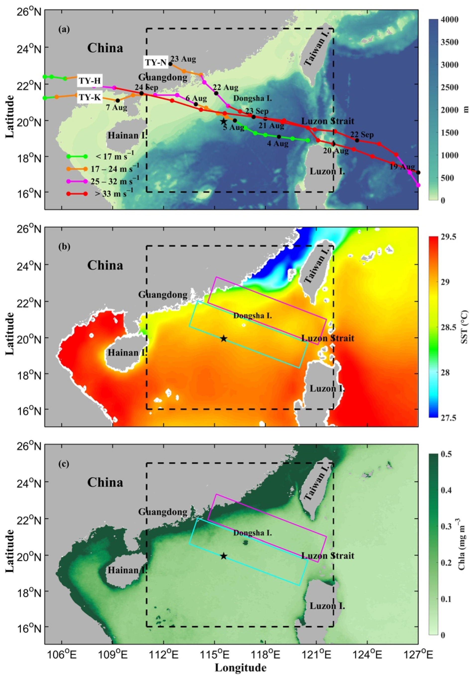
2.1. Typhoon Feature and Tracks

The typhoon best-track data used in this study are available from the Japan Meteorological Agency (JMA). These datasets include date and 6 h information on typhoons, i.e., category, locations, central pressure, maximum sustained wind (MSW) speed (1 min mean maximum sustained wind speed at 10 m height), and maximum radii of 30 and 50 knot winds. JMA best-track reported times and locations were used to calculate the translation speed ($U_h$) of the typhoons [3] as the ratio between the distance traveled between two sequential times and the corresponding time period, i.e., 6 h.

A total of 22 tropical cyclones in the western Pacific were reported by the JMA in 2008, and three of these cyclones, i.e., Kammuri, Nuri, and Hagupit, were investigated in this study (

Table 1. Basic information on the three typhoons.

Typhoon Name (ID)	Kammuri (ID: 0809)	Nuri (ID: 0812)	Hagupit (ID: 0814)
Start and end date	3–8 August	17–23 August	17–23 September
Maximum sustained wind speed (m s−1)	25.7 (00:00–06:00 6 August)	38.6 (06:00 19 August to 18:00 20 August)	46.3 (18:00 23 September)
Mean translation speed (m s−1) in study region	4.2	4.7	8.0
Averaged radius (km) with wind speed > 27 m s−1	/	67.0	82.3
Averaged radius (km) with wind speed > 15 m s−1	185.5	179.0	224.5

, Figure 1a). The first typhoon, Kammuri, originated as a tropical depression to the north of Luzon Island on 3 August 2008, moved at a steady slow speed (3.0–3.9 m s⁻¹) and weak intensity (less than 24 m s⁻¹) over the northern SCS from 4–5 August, reached its peak wind speed of 25.7 m s⁻¹ on 6 August, and finally made landfall on mainland China in western Guangdong [36]. The second typhoon, Nuri, formed in the western North Pacific on 17 August 2008, propagated westward at a relatively fast translation speed, e.g., between 3.7 m s⁻¹ and 6.2 m s⁻¹, with a persistent high intensity of 33 m s⁻¹ or higher, until its landfall in Guangdong on 22 August. The third typhoon, Hagupit, developed as a tropical depression (wind speed less than 32 m s⁻¹) on 17 September in the western North Pacific and strengthened during its rapid propagation (i.e., 8 m s⁻¹) toward the northwest. The intensity peaked at a wind speed of 46 m s⁻¹ on 23 September and decreased after making landfall in Guangdong on 24 September, making it one of the strongest typhoons at landfall in recorded history.

These typhoons were separated in time and occurred in diverse oceanic conditions, and the evolution of typhoon wakes could be studied with limited interference by subsequent typhoons. However, they had similar tracks in the northern SCS, where both ACEs and CEs occur. These tracks resulted in complex ocean conditions with distinctive dynamic responses. The case studies emphasize how varying intensity, translation speed, and initial oceanic conditions (i.e., mesoscale eddies) influence the response of the upper ocean.

Climatologically averaged oceanic features over the period from 1 August to 8 October showed that the chlorophyll (Figure 1b) and temperature (Figure 1c) along the trajectories of all typhoons were uniformly distributed. There was limited spatial variation in the values, except in the coastal regions where the chlorophyll (temperature) was prominently higher (slightly lower) than that in the surrounding regions. Thus, the typhoons are expected to have experienced limited variation in the underlying oceanic conditions during their passage.

2.2. Dataset of Oceanic and Atmospheric Features

Measurements of wind and SST data are used to study the oceanic and atmospheric variations in the three typhoons. In situ observations for wind speed were obtained at a mooring buoy (MB), which was deployed at 19.95°N, 115.53°E with a depth of 1500 m (Figure 1). The buoy had a height of 5 m and a diameter of 3 m and weighed approximately 1500 kg. The MB was equipped with R. M. Young (05106-L) and Campbell Scientific (107-L) devices to measure wind and temperature, respectively. Both sensors were located at a height of 3 m above the ocean surface, and the wind measurements were adjusted to a height of 10 m above sea level. According to Smith [37], the wind speed (U) at measurement height z is determined as

$$U=\frac{u_{*}}{K}\ln \left(\frac{z}{z_0}\right)$$

(1)

where $u_{*}$ is the friction velocity, κ is the von Karman constant (0.4), and $z_0$ is the drag coefficient, obtained by

$$z_0=\alpha \frac{u_{*}^2}{g}+\beta \frac{v}{u_{*}}$$

(2)

where $\alpha$ is the Charnock constant (0.024) [38], g is the acceleration of gravity (9.8 m s⁻²), $\beta$ is the limiting roughness (0.11), and $v$ is the viscosity of air (14 × 10⁻⁶ m s⁻¹). Substituting the buoy-measured wind speed and the measurement height (3 m) into Equation (1) and combining Equations (1) and (2) yields $u_{*}$ and $z_0$ iteratively. Finally, all buoy wind speeds were converted to a neutral wind data height of 10 m, $U_{10}$, which was estimated from Equation (1) at z = 10 m for the derived $u_{*}$ and $z_0$ [39].

The wind field, SST, and barometric pressure data were simultaneously measured at hourly intervals from 1 July 2008 to 30 July 2010, but the sensor failed on 8 March 2010. The observations were smoothed by taking the running average over every 24 measurements. Due to battery failure and buoy replacement, there are some gaps in the observations for SST and wind field, but observations are available for at least two typhoons.

Satellite measurements of the wind field were obtained by the Quick Scatterometer (QuikScat) with a horizontal spatial resolution of 0.25° × 0.25°, which was distributed by Remote Sensing Systems (RSS). The daily QuikScat wind field data, which are obtained first by averaging the measurements of the corresponding ascending and descending tracks, successfully captured the wind structure and intensity of the three typhoons. The wind stress $\overrightarrow{\tau }$ on the ocean surface is then estimated based on daily wind velocities via the following bulk formula:

$$\overrightarrow{\tau }={\rho }_a{C}_d{u}_{10}\overrightarrow{u_{10}}$$

(3)

where ${\rho }_a$ is the density of air (1.25 kg m⁻³), $u_{10}$ is the wind speed at the 10 m height, and $\overrightarrow{u_{10}}$ is the wind vector. The drag coefficient ($C_d$) was calculated following Oey et at. [40]. Briefly, the coefficient is defined as follows:

$$\begin{array}{c}{C}_d\times {10}^3=1.2, U_{10}\le 11 {\mathrm{m} \mathrm{s}}^{-1}\\ 0.49+0.065U_{10}, 11<U_{10}\le 19 {\mathrm{m} \mathrm{s}}^{-1}\\ 1.364+0.0234U_{10}-0.0002U_{10}^2, 19<U_{10}\le 100 {\mathrm{m} \mathrm{s}}^{-1}\end{array}$$

(4)

The wind stress is spatially smoothed by averaging 3 pixels by 3 pixels to reduce small-scale motions, leading to a reduced wind stress compared with the reported numbers (Table 1).

To present the spatiotemporal variation in wind-induced upwelling with the passage of the three typhoons, the Ekman pumping velocity (EPV), which reflects the upwelling intensity, is calculated from the daily QuikScat wind vector product as follows [41]:

$$W_E=\frac{1}{\rho f}\left(\frac{\partial {\tau }_y}{\partial x}-\frac{\partial {\tau }_x}{\partial y}\right)$$

(5)

where W_E is the EPV and ${\tau }_x$, ${\tau }_y$, $\rho =1020{ \mathrm{kg} \mathrm{m}}^{-3},$ and $f$ are the zonal and meridional components of wind stress on the sea surface, sea water density, and the Coriolis parameter, respectively.

Daily SST data with a resolution of 9 km were also obtained from RSS. We used SST products that were integrated with microwave (MW) and infrared (IR) data. The daily spatial distributions of the SST were analyzed to indicate the changes in water temperature associated with the three typhoons.

To investigate the spatial and temporal variations in phytoplankton biomass at the sea surface, daily Level 3 remotely sensed surface Chl-a concentrations with a spatial resolution of 4 km, developed by the European Space Agency’s (ESA) Ocean Color Climate Change Initiative (OC–CCI), are used in this study. These data are a combination of Moderate Resolution Imaging Spectroradiometer (MODIS) Aqua, Visible Infrared Imaging Radiometer Suite (VIIRS), and Sea-Viewing Wide Field-of-View Sensor (SeaWiFS) datasets [42].

The daily sea-level anomaly (SLA) datasets with 0.25° × 0.25° spatial resolutions were obtained with Archiving, Validation and Interpretation of Satellite Oceanographic Data (AVISO) from the Copernicus Marine Service (CMEMS). These products incorporate data from the TOPEX/Poseidon, ERS-1, and ERS-2 altimeters. Eddy datasets were distributed by the altimetric Mesoscale Eddy Trajectories Atlas (META2.0), which was mainly conducted using AVISO. The dataset includes the polarity, i.e., CE or ACE, central location, speed, and radius for each eddy at daily intervals. Because the study region is very close to the coastline, some adjustments were conducted using the SLA data for identifying continuous trajectories of eddies following Chelton et al. [43] and Pegliasco et al. [44].

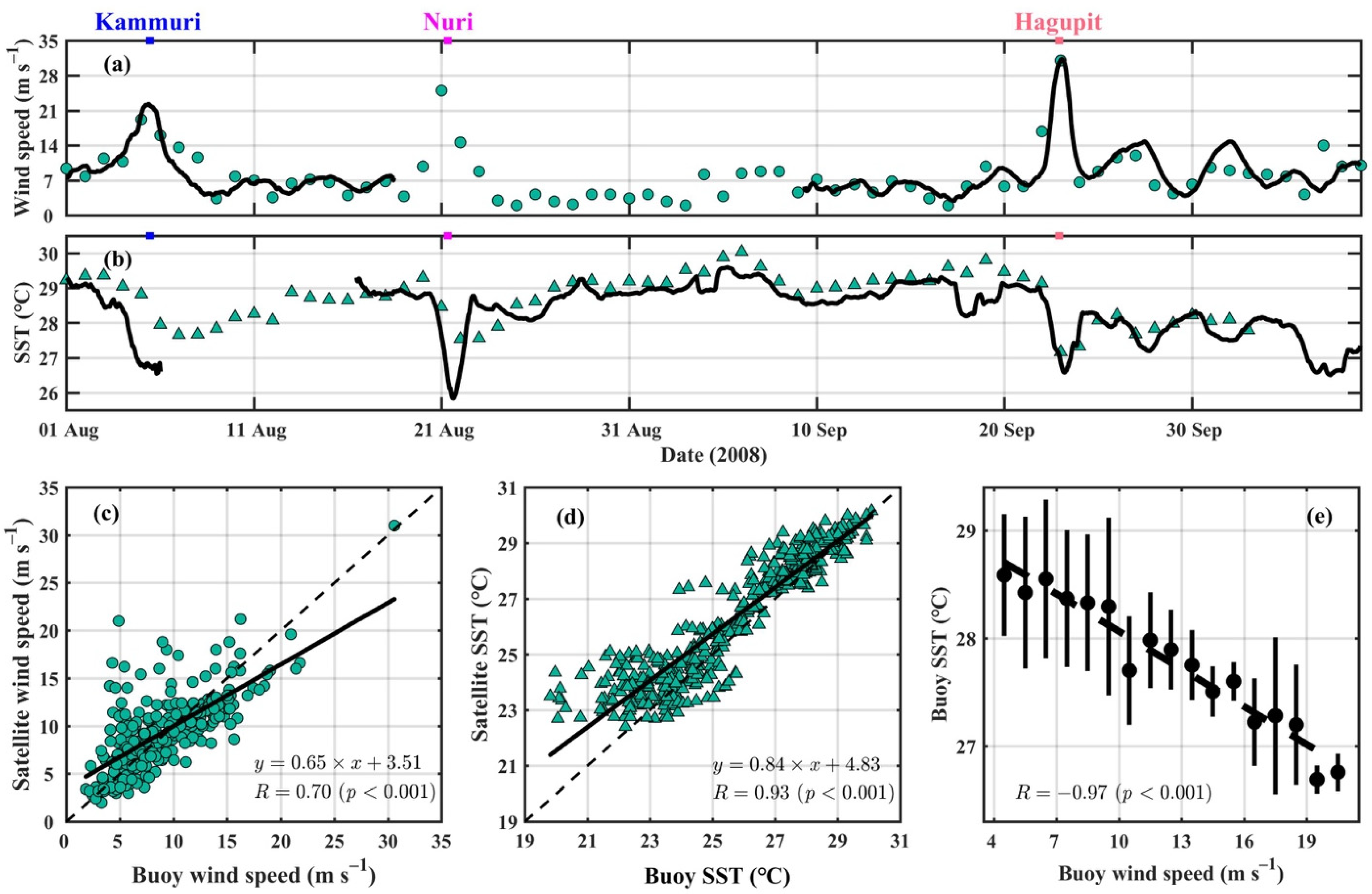
2.3. In Situ Observations and Validation of Remotely Sensed Data

Remotely sensed ocean surface features during the typhoon passages were validated by comparison with the in situ observations. Daily satellite observations were first spatially averaged over 1°, centering at the location of the MB. The time series was highly consistent between both observations (Figure 2). In particular, the wind speed was weak (approximately 7 m s⁻¹) before and after each typhoon, while it increased during each typhoon. The peak wind speed was highest during Hagupit, followed by Nuri and lowest during Kammuri. The instantaneous wind speed and SST measured by the in situ buoy are highly comparable to the satellite observations (Figure 2c,d). The temperature observed by the buoy is slightly lower than the satellite-observed SST, which is probably because the equipped temperature sensor was located above the ocean, where the air temperature was slightly lower than the water temperature. The temperature cooled in association with the increase in wind field, reached the lowest value within 2 days after the peak values of typhoon winds, and gradually recovered after typhoons in a week or so. The largest cooling occurred after Typhoon Nuri, while the cooling was comparable after the other two typhoons.

The measurements of wind speed and SST from satellite observations were validated by comparison with in situ observations, and significant linear regressions were identified between them (Figure 2c,d). Similarly, the QuikScat dataset was also validated by comparison with in situ measurements in the Mediterranean basin [45]. Although there are gaps in the buoy data during Typhoon Nuri, less than 10% of the total data is missing, indicating a minor impact on the credibility of the in situ observations. A scatterplot (Figure 2c) shows that the QuikScat wind speed was close to that of buoy; this is especially true when the wind speed was 5–15 m s⁻¹, even for the single highest wind speed (~31 m s⁻¹) during Typhoon Hagupit (Figure 2a,c). The scatterplot (Figure 2d) between buoy SST and satellite SST shows perfect consistency, and the slope of the regression is very close to 1 with a correlation coefficient of 0.93. Overall, the measurements of the buoy and satellite are in great agreement, and their linear regressions are significant at the 99% confidence level. The corresponding root mean square errors are 3.30 and 1.12 for wind speed and SST, respectively. The validated satellite observations are applied in this study to investigate the oceanic response during typhoons, especially considering that buoys do not have the ability to make large-scale observations.

On the other hand, intensive cloud coverage can block satellite observations over the oceanic surface. Many previous studies have shown that satellite observations are usually absent at the time of a typhoon’s passage [3]. Thus, the validation of satellite observations during the passage of a typhoon should be comprehensively assessed before using remotely sensed data. For example, Chai et al. [21] compared biogeochemical-Argo observations with satellite observations and found that chlorophyll measured by satellites is not available due to cloud coverage and underestimates the typhoon’s impact with satellite data. In comparison, the observed SST is consistent with in situ observations that the satellite data can be applied to gauge the typhoon-induced oceanic responses. The wind speed and SST distribution along the diagonal can be used to estimate the degree of matching during different periods, especially during typhoon and nontyphoon periods.

The daily wind field and SST from in situ observations were further investigated to assess their dependence, and a prominent linear relationship was identified (Figure 2e). Stronger winds were accompanied by lower temperatures, indicating that typhoon-induced mixing led to upper ocean cooling [21]. The dependence was persistently valid when the wind was leading the temperature by 1–2 days because the typhoon’s impact on the temperature lasted for a few days [11]. Yu et al. [2] identified a dependence on monsoon wind and other parameters, e.g., SST and Chl-a, in the seasonal cycle, which may not be reflected here, although a two-month time span was applied in this study. This was mainly because the climatological features were mostly stable from August to September [3], but the identified large variation was much greater than the seasonal changes.

3. Results

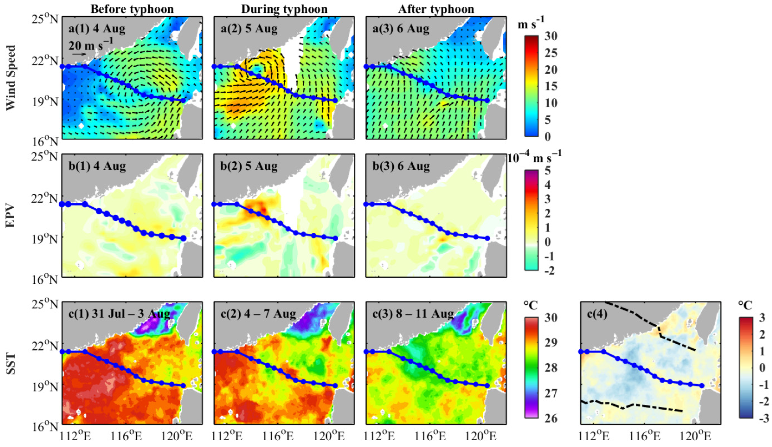
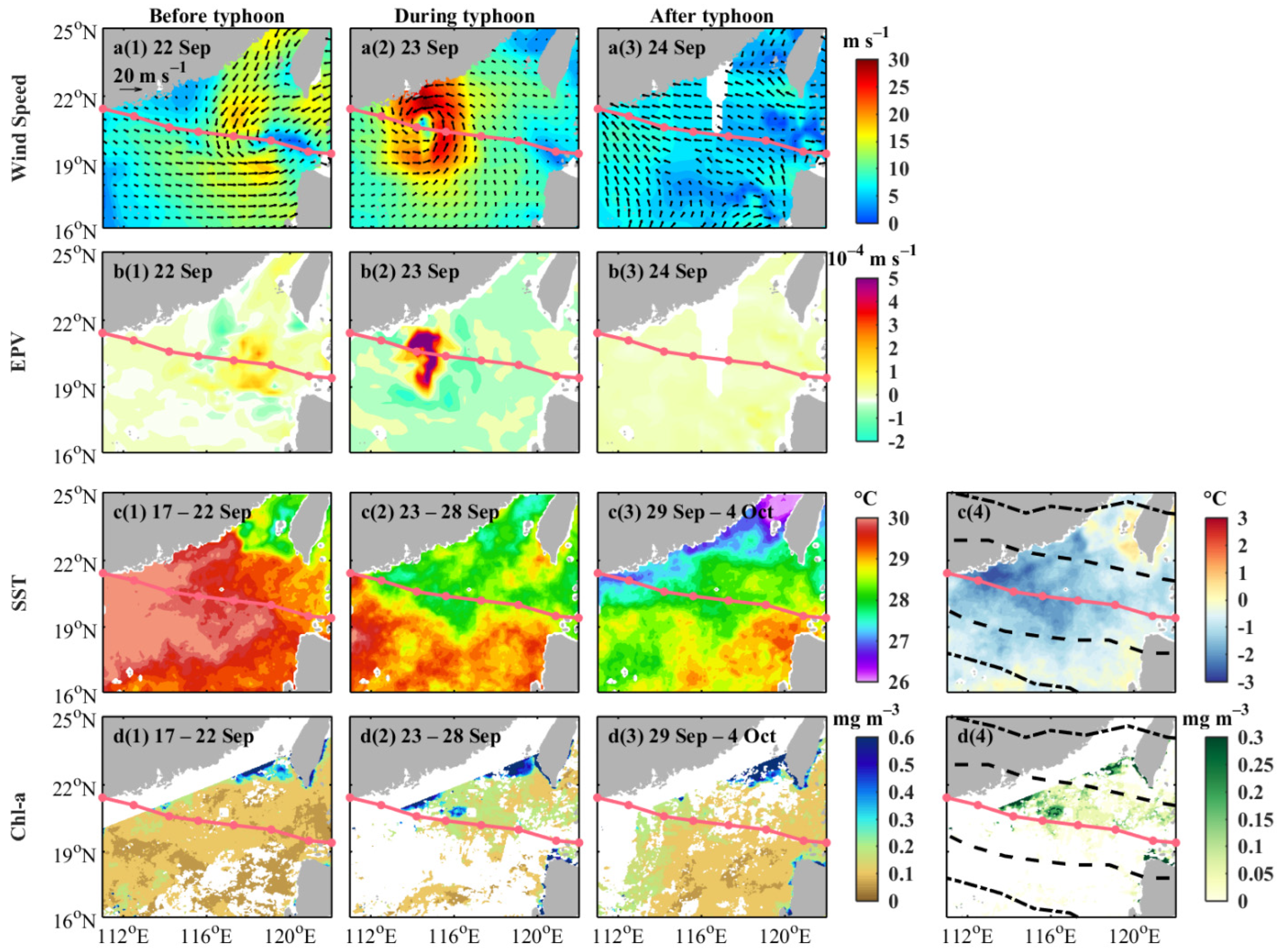
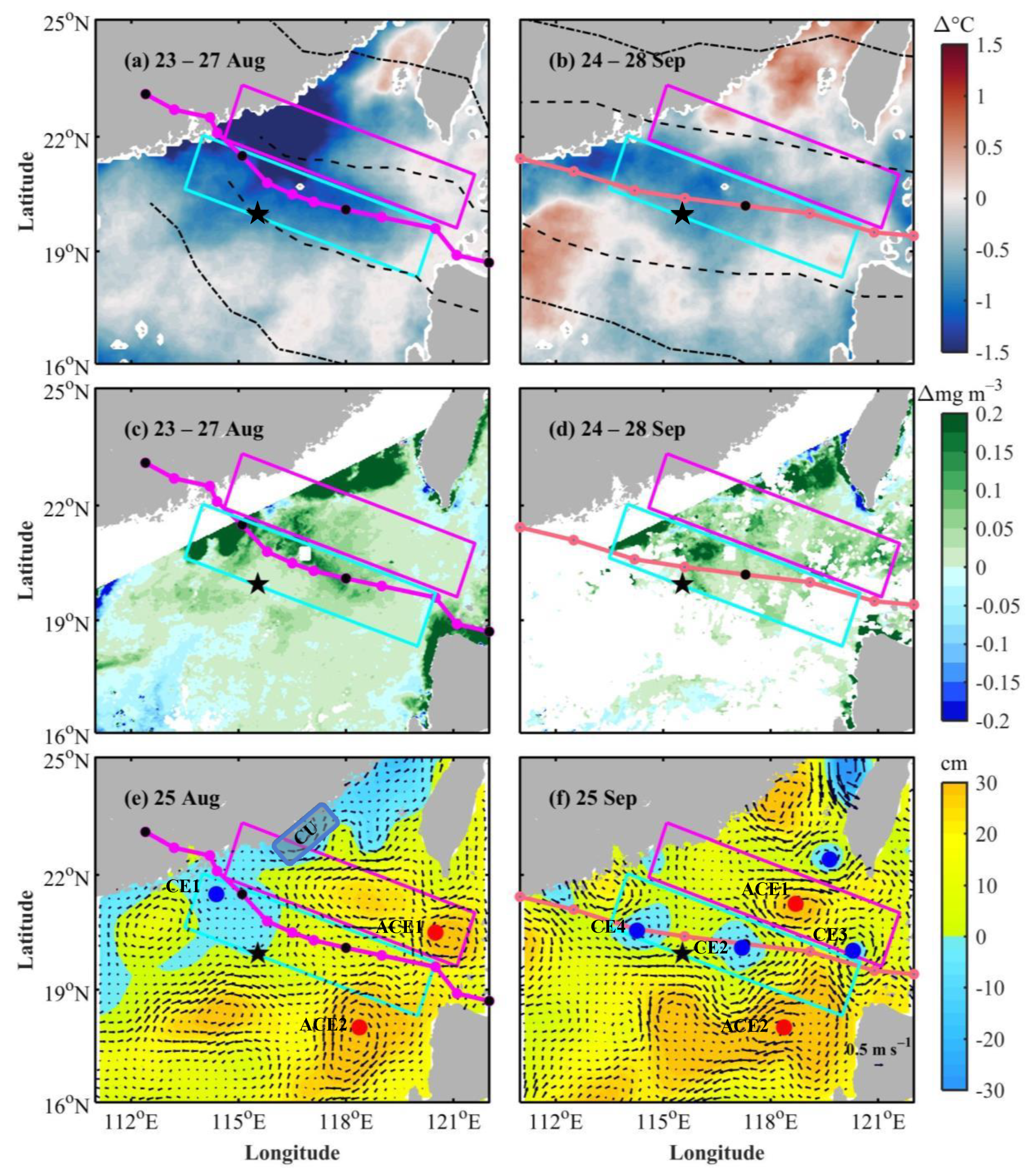
3.1. Spatial Pattern of Typhoon and Typhoon-Induced Changes

To quantitatively investigate the influence of the three typhoons on oceanic conditions, the spatial distributions of the wind field, EPV, SST, and Chl-a are studied. Specifically, the spatial distributions of wind speed and EPV on three successive days, centered on the date when the typhoon reaches its maximum intensity, are shown, while temporal averages of SST and Chl-a are applied before, during, and after each typhoon. The Chl-a pretyphoon is generally below 0.1 mg m⁻³ in the open basin, e.g., 100 km away from the coast, consistent with the typical summer surface [2]. In contrast, the Chl-a in nearshore regions is generally more than 0.6 mg m⁻³. Typhoon-induced vertical mixing and upwelling are evident in the upper ocean; thus, sea surface cooling and Chl-a enhancement are studied by comparing SST and Chl-a before and after typhoons. Specifically, this study applies the anomalous field, which is defined as the difference between the time series and corresponding climatology, to study the typhoon-induced variation.

The northern SCS was characterized by weak northward winds in the summer of 2008, similar to the climatological conditions [2]. Typhoon Kammuri was characterized as a westward-propagating anti-clockwise wind field (Figure 3a) associated with a weak positive EPV, which is favorable to upwelling (Figure 3b). On 5 August, the wind field was distributed asymmetrically around the typhoon center, with the highest daily average wind speed, which exceeded 17 m s⁻¹ to the right of the track (Figure 3(a2)). As a slow-moving and weak typhoon, there was a positive EPV along the track of Kammuri. The corresponding SST decreased along the track of Typhoon Kammuri with no significant difference between its left and right sides (Figure 3c). Low SSTs of 28.0–29.0 °C appeared within 100 km on both sides of the track during its passage; subsequently, a minimum SST (27.5 °C) was identified to the right of the track, associated with an SST decrease of approximately −1.5 °C (Figure 3(c4)). SST cooling occurred roughly within the area where the wind speed of the typhoon was greater than 15 m s⁻¹. Because intensive cloud coverage can interfere with Chl-a observations, the corresponding data are not shown.

When Typhoon Nuri entered the SCS from the Luzon Strait on 20 August, it moved slowly (3.4 m s⁻¹) and featured weak winds (<14 m s⁻¹) and low EPVs (<2 × 10⁻⁴ m s⁻¹) on both sides of the track (Figure 4(a1,b1)). The wind speed increased greatly to 33 m s⁻¹ on 21 August, with high EPVs observed on both sides of the track (Figure 4(a2,b2)), consistent with the findings in [10]. The wind speed and EPV decreased greatly after the passage of the typhoon (Figure 4(a3,b3)). SST cooling was detected to the right of the track during its passage (Figure 4(c2)). A minimum value of 27.3 °C was identified at the center (118.9°E, 19.9°N) of a cold pool, indicating intense SST cooling of approximately −2 °C to the right of the typhoon track (Figure 4(c4)). A strong wind stress curl induced seawater upwelling during the passage of Nuri, resulting in significant enhancement of the entrainment of subsurface water and the oceanic response [7]. The SST returned to 29.0–30.0 °C to the left of the track but remained below 29.0 °C to the right of the track after the typhoon’s departure (Figure 4(c3)). A bloom patch (115–117°E, 20.5–22°N) with an average surface Chl-a of 0.3 mg m⁻³ was observed on the right side of Nuri’s track (Figure 4(d2)). The corresponding value was substantially larger than that before the typhoon (Figure 4(d4)) and the climatology [11]. The spatial area with SST cooling basically fell within the region where the typhoon’s wind speed was greater than 15 m s⁻¹, but the region with Chl-a enhancement was much smaller, corresponding to the area where the typhoon’s wind speed was mostly greater than 27 m s⁻¹.

Typhoon Hagupit was characterized by the highest translation speed of 8.0 m s⁻¹ among the three typhoons. An anti-clockwise wind field with a peak wind speed of 30 m s⁻¹ occurred on 23 September (Figure 5a). The EPVs derived from the wind stress reveal weak but persistent upwelling conditions (Figure 5b), with EPV values higher than 5 × 10⁻⁴ m s⁻¹ on 23 September along Hagupit’s path (Figure 5(b2)). The averaged SST before Hagupit was predominantly high (Figure 5(c1)), and a distinct cold patch was observed during the passage of the typhoon (Figure 5(c2)), with a minimum value of 28.3 °C near its track (118.9°E, 19.9°N). The maximum cooling of −3.0 °C occurred on the right side of the typhoon track (Figure 5(c4)) and was greater than that induced by Nuri (Figure 5(c4)). After the passage of Hagupit, the SST near the coast was prominently below 27 °C, and the offshore SST maintained similar values during the typhoon (Figure 5(c2,c3)). The cooling was associated with an increase in Chl-a, and Chl-a enhancement reached approximately 0.3 mg m⁻³ on 26 September at 116.2°E, 20.9°N to the right of the track. Similar to the conditions following Typhoon Nuri, the spatial range of SST cooling was much larger than that of Chl-a enhancement.

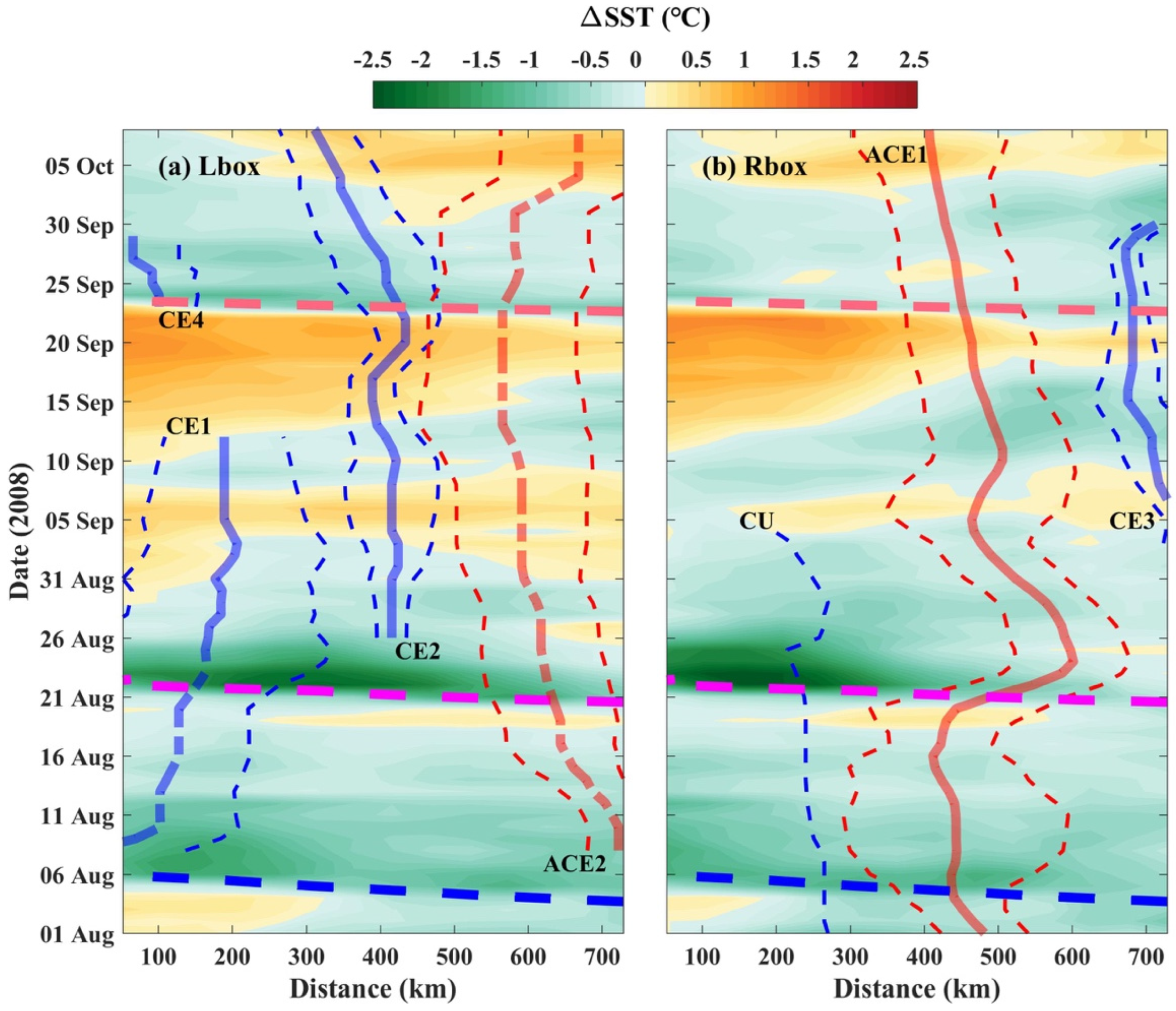
3.2. Eddy-Modulated Ocean Surface Changes along the Typhoon Track

Notably, strong enhancements in Chl-a are located to the right of the tracks of Nuri and Hagupit (Figure 4(d4) and Figure 5(d4)), consistent with the upwelling regions in Figure 4b and Figure 5b. The phytoplankton bloom lasted for a pronounced period, i.e., 5–7 days, before fading, which may have been due to the existence of mesoscale eddies. The eddies and their impacts on modulating the typhoon-induced changes were examined via satellite observations. Two regions along typhoon tracks were applied for further investigation, and the majority of the typhoon-induced anomalies at the ocean surface were included. The anomalous field was defined as the difference between the observed feature and the corresponding climatology. The averaged anomalous SST (ΔSST, Figure 6a,b) and Chl-a (ΔChl-a, Figure 6c,d) are shown after the passages of Nuri from 23 to 27 August and Hagupit from 24 to 28 September. Both boxes cover roughly the same area of approximately 1.18*10⁵ km² but are located on each side of the typhoon; specifically, the cyan box (Lbox) and purple box (Rbox) are located to the left and right of the general tracks of the typhoons, respectively. Snapshots of the SLA field and derived geostrophic current on 25 August and 25 September were overlaid with the simultaneous locations of eddy centers (Figure 6e,f). The information on both regions and all eddies is summarized in

Table 2. Information on the two boxes and eddies during the passage of the typhoons (Lbox: cyan box; Rbox: purple box; CE: cyclonic eddy; ACE: anticyclonic eddy).

Box	Location of Vertices	Eddy	Eddy Center Location	Period of Eddy	Mean Radius of Eddy (km)	Existence of Eddy during Typhoon
						Kammuri	Nuri	Hagupit
Lbox	23.3°N, 115.1°E; 21.9°N, 114.6°E; 19.6°N, 121.1°E; 21.0°N, 121.6°E	ACE2 *	117.93°E, 17.89°N	1 August–8 October	82	Y	Y	Y
		CE1	114.90°E, 20.44°N	9 August–12 September	112	N	Y	N
		CE2 *	117.12°E, 20.19°N	26 August–31 October	47	N	N	Y
		CE4	114.27°E, 20.55°N	23–29 September	57	N	N	Y
Rbox	22.0°N, 114.0°E; 20.6°N, 113.5°E; 18.3°N, 120.0°E; 19.7°N, 120.5°E	ACE1 *	118.79°E, 21.18°N	28 May–8 October	89	Y	Y	Y
		CE3 *	120.54°E, 19.90°N	3–30 September	29	N	N	Y

* SLA data were applied to confirm that multiple eddies identified from the META dataset were the same.

.

Typhoon-induced changes were captured in both boxes and included patches of cold SSTs and high Chl-a observed along the typhoon tracks with slightly higher values to the right (Figure 6). The spatial patterns were related to the pre-existence of eddies. For example, the maximum cooling (−1.7 °C) occurred due to the impact of a CE (CE1) and coastal upwelling during the passage of Nuri (Figure 6c,e). In contrast, persistent ACEs, e.g., ACE1, reduced the impact of typhoons where both ΔSST and ΔChl-a were minimal (Figure 6a,c,e).

To further examine the effect of eddies on the impact of typhoons on SST, Hovmöller diagrams of ΔSST at different distances from the coast are investigated over the period from 1 August to 8 October 2008, in each box (Figure 7). The locations of eddy centers and the corresponding radius are overlayed in the figures. The SST cooling significantly varied in response to both typhoons and eddies. Before the arrival of Typhoon Kammuri, CE1 was generated, but its center was located to the west of the Lbox. The SST decreased slightly (−1.4 °C) after the passage of Kammuri from 6–10 August in the western Lbox under the impact of CE1. The cooling was still more prominent than that in the Rbox because the impact of CEs and typhoons was further from the Rbox. After Kammuri’s departure, the eddy center of CE1 entered the Lbox. SST decreased greatly in both boxes, e.g., −2.5 °C, after Nuri’s passage on 23 August, due to the impact of CE1 and enhanced coastal upwelling (CU) in the Lbox and Rbox, respectively. Because of the pre-existing ACEs, e.g., ACE1 and ACE2, cooling was much less prominent on the eastern side. SST cooling lagged the maximum wind speed by two days (Figure 2a,b) and tended to be more prominent to the right of Nuri’s track (Figure 4c and Figure 7b). After the departure of Nuri, the SST rebounded in both boxes, but the warming was slower in regions with CEs. The SST decreased after the passage of Typhoon Hagupit on 23 September but with less intensity, e.g., approximately −1.0 °C, from 24–29 September, due to the rapid movement of the typhoon. The cooling was slightly larger in the region under the impact of CEs, e.g., CE4 and CE2 in the Lbox and CE3 in the Rbox.

The typhoon-induced ΔSST and ΔChl-a were further investigated for their dependence on the wind field. Both boxes were spatially divided into 14 bins with different offshore distances. The ΔSST, ΔChl-a, and wind speed during the period when typhoons passed over were averaged in each bin. Note that the wind was obtained using the date when typhoons passed over, but the applied dates of ΔSST and ΔChl-a were one day and three days lagged, respectively, relative to the wind field due to the time required for the greatest oceanic responses [3]. Negative dependences were identified in all cases with significant regressions, in which greater cooling was associated with stronger wind (Figure 8). The ΔSST in the Lbox was evidently negative within CE1 after Typhoon Nuri, e.g., −1.8–−2.3 °C, and within CE4 after Typhoon Hagupit, e.g., −0.9–−1.2 °C. Additionally, cooling was prominent in the Rbox with the impact of CU after Typhoon Nuri, e.g., −2.0–−2.5 °C. In contrast, ΔSST was much smaller inside ACE1 and ACE2, with values less than −0.8 and −1.5 °C, respectively, after Typhoon Nuri and less than −0.6 °C inside ACE2 after Typhoon Hagupit. During nontyphoon periods, the ΔSST was generally characterized as a neutral status with a value bounded by that impacted by CE and ACE. Due to the complex dynamics, there were some cases where the typhoon-induced changes did not follow the identified pattern, e.g., weak cooling was found in CE3 (Figure 8d).

A similar approach was applied to investigate the dependence between ΔChl-a and the wind field. The peak value of Chl-a appeared within a week of Nuri’s and Hagupit’s passages (Figure 4); thus, the average of ΔChl-a was calculated using the time that was three days after the passage of the typhoons. A positive dependence was generally identified between ΔChl-a and wind speed (Figure 9), indicating that strong wind introduced more nutrients or redistributed the subsurface Chl-a maximum within the mixed layer [21]. Large variance was identified in both boxes, and some regressions were not statistically significant, but the effect of eddies on typhoon-induced Chl-a changes was still recognizable. For example, the changes in ΔChl-a inside CEs were generally larger than those without eddies or within ACEs. Additionally, the region with CU also showed anomalously high ΔChl-a values. Specifically, the largest change in ΔChl-a was identified within CE1, CE4, and CU. In contrast, the smallest change in ΔChl-a was identified within ACE1 and ACE2. The maximum ΔChl-a inside CE4 was ~0.4 mg m⁻³ due to the coeffect of a CE (23–29 September), CU, and the passage of Hagupit in the Lbox (Figure 9c). Similarly, the ΔChl-a inside the CU region was ~0.12–0.24 mg m⁻³ because of the CU during Nuri in the Rbox (Figure 9c). Furthermore, the ΔChl-a inside CE1 was ~0.09–0.17 mg m⁻³, which was obviously affected by a CE after the passage of Kammuri and during the passage of Nuri (Figure 9a). Compared with typhoon-induced SST changes, there was much more variation in Chl-a due to complex dynamic and ecological processes [10].

4. Discussion

4.1. Dynamics Determine Typhoon-Induced upper Ocean Responses

The study of factors affecting upper ocean responses to typhoons in offshore areas is fundamentally important. Based on the three typhoons with similar tracks but different intensities, the complex dynamic processes of the interaction between the atmosphere and the ocean in the northern SCS were investigated. During summer and autumn, the high SST in the SCS generally enhances stratification in the upper ocean, while weak winds produce weak vertical mixing [2]. There is considerable spatiotemporal variation in Chl-a, and regions with large typhoon-induced changes were located in offshore areas, where the water depth is 200–3000 m (Figure 1); therefore, the resuspension of bottom materials and riverine input on Chl-a blooms was limited and can be ignored in the study area. Thus, a low Chl-a pattern (<0.1 mg m⁻³) is observed in offshore areas without the presence of typhoons.

Satellite observations during typhoon passage are well validated with the in situ MB dataset (Figure 2) and can present reliable information for quantitatively depicting oceanic responses. In particular, SST cooling is largely related to the strong winds of typhoons (Figure 2c). Strong winds (>8 m s⁻¹) were observed over the entire northern SCS, with the highest wind speeds (>30 m s⁻¹) being identified near the tracks of typhoons Nuri (Figure 4(a2)) and Hagupit (Figure 5(a2)). In addition, stronger upwelling (>5.0 × 10⁻⁴ m s⁻¹) was seen during typhoons Nuri and Hagupit (Figure 4(b2) and Figure 5(b2)). The spatial distribution roughly matched the patch of SST cooling (Figure 4(c2) and Figure 5(c2)) with right-side intensification [7]. In contrast, there was weak upwelling (<2 × 10⁻⁴ m s⁻¹) during Kammuri (Figure 3(b2)), and cooling was also less prominent.

Past studies have demonstrated that upper ocean responses are intensified with the increasing intensity and decreasing translation speed of typhoons [5,7]. Strong winds and intensified upwelling decrease the SST and supply nutrients from the subsurface layer to the euphotic zone, inducing an extensive increase in phytoplankton [3]. Fast-moving typhoons, i.e., those with translation speeds greater than 6 m s⁻¹, can strengthen to high intensities when the surface warm layer is shallow, while slow-moving typhoons require much deeper surface layers in order to intensify [34]. Thus, the negative feedback resulting from a typhoon’s self-induced cooling can be effectively limited with a fast translation speed [46], while the negative feedback is enhanced for slow-moving typhoons [15,47]. Our results suggest that wind-induced upwelling transports deep and nutrient-rich water into the upper layer and subsequently triggers phytoplankton blooms in the study region. These results agree with those of Ye et al. [11], who showed that upwelling water rich in nutrients at 20–100 m depth induced a Chl-a bloom, and a maximum value of Chl-a was found during Nuri. Thus, such nutrient-rich waters can be critical to offshore blooms. In contrast, Typhoon Hagupit, despite its higher wind speed, did not have such strong effects on the upper ocean due to its faster translation speed (8.0 m s⁻¹) and short forcing time. The full development of the potential wind-induced upwelling velocity and mixing requires a time period longer than the geostrophic adjustment time (i.e., the inertial period) [48]. The forcing time of Nuri (~60 h) was much longer than the inertial period and therefore resulted in a fully developed upwelling system. The spatial range of a typhoon is also an important factor in determining the ocean’s response [49]. Nuri was large, with the area with wind speeds of 27 m s⁻¹ having a radius of over 50 km (Figure 4); thus, the cumulative effect of typhoon-induced entrainment and upwelling were significant. Indeed, the influence of Nuri on SST was most prominent in this region. In comparison, the influence of typhoons on Chl-a was more complex, with notable Chl-a increases after the passage of Nuri and Hagupit, and the change in Chl-a was simultaneously related to the existing eddies [19,50], which is discussed in the following section.

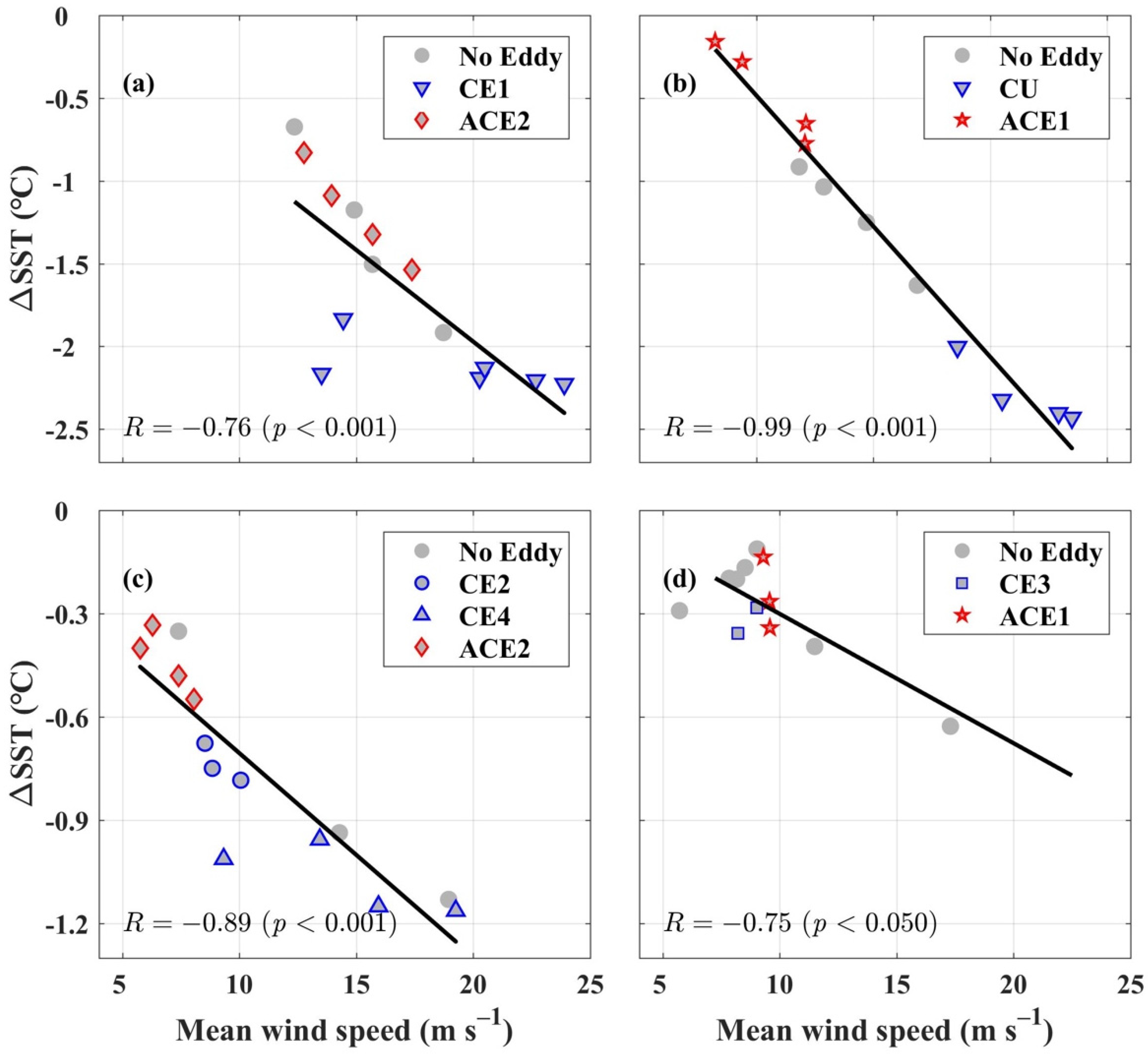
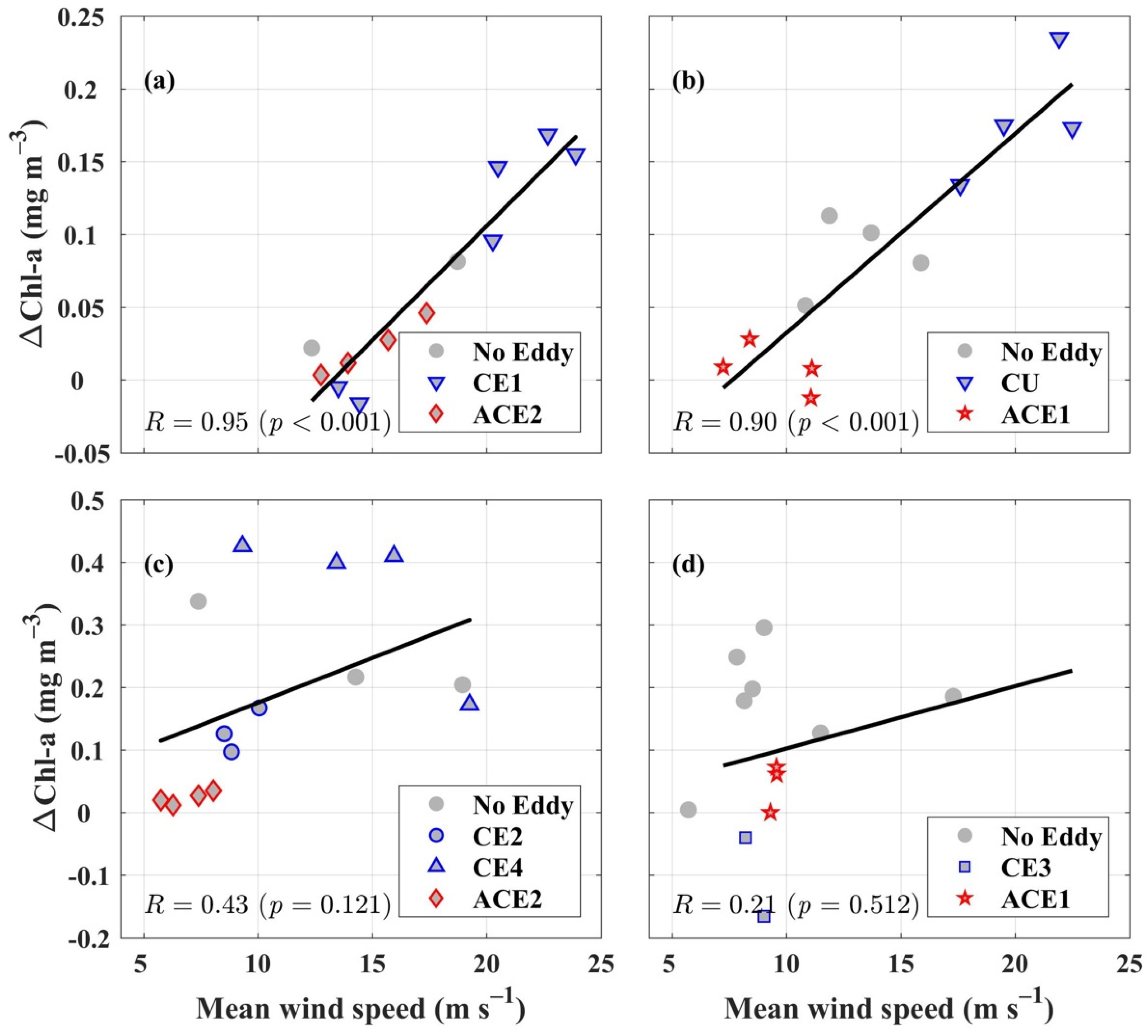
4.2. Modulation of Typhoon-Forced Oceanic Responses by Pre-Existing Mesoscale Eddies

A tropical cyclone can induce upwelling, which can be further enhanced by a CE and subsequently fuel phytoplankton blooms. Thus, it is important to describe how a typhoon-enhanced CE modifies the oceanic response, e.g., SST cooling and phytoplankton blooms. The present study captured cooling and phytoplankton blooms coincident with mesoscale eddies and typhoons (Figure 7). The mechanisms of the upper ocean responses along the trajectories of typhoons are illustrated with the statistical relationship (Figure 8 and Figure 9).

As Typhoon Nuri passed over, it induced vigorous upwelling and vertical mixing with a maximum upwelling velocity much higher than 5.0 × 10⁻⁴ m s⁻¹ and a wind speed of 38.6 m s⁻¹. Ye et al. [11] compared Chl-a before and after Typhoon Nuri and showed that Chl-a was influenced by a CE and that the enhancement in Chl-a persisted for almost three weeks (28 August to 15 September). Consistently, we also found prominent typhoon-induced Chl-a enhancement and further identified that its spatial pattern was largely related to the occurrence of pre-existing eddies. In particular, high ΔChl-a values occur in association with CEs, while low ΔChl-a values occur in association with ACEs (Figure 9).

Satellite images of SST (Figure 4(c4)) show a core of cooling extending from 20°N to 22°N and from 114°E to 116°E, with a diameter of approximately 100 km. The surface Chl-a was almost three times higher than that before the typhoon, and these high levels lasted for 5 days. The images of Chl-a also show an area of surface enhancement coinciding with the cooling core (Figure 4(c4)). Due to the asymmetric wind forcing of typhoons [7,10], the surface Chl-a enhancement to the right of Nuri’s track was higher than that to the left (Figure 4(d4)). The existence of a CE also strengthened the upper ocean responses by increasing the nutrient supply during and after the typhoon passage [34,51,52]. Sea surface cooling, accompanied by a sea-level decrease along the track of Nuri, indicates upwelling associated with a CE [8] (Figure 4). The typhoon-induced oceanic responses are enhanced by CEs, e.g., CE1 during Typhoon Nuri and CE4 during Typhoon Hagupit (Figure 8 and Figure 9). A time lag between the typhoon and the largest oceanic changes, e.g., 1 day for SST and 3 days for Chl-a, is consistent with the time required for the physics and biology to respond to extreme wind fields [53], while the prolonged changes are attributed to the impact of mesoscale eddies [35].

The study reveals that mesoscale eddies can significantly modulate the typhoon’s impact on the upper ocean by modifying the upwelling and vertical entrainment [54]. As cold water with more nutrients is supplied to the euphotic zone, the SST is depressed, and Chl-a increases along the typhoon track, exhibiting enhanced patches associated with CEs (Figure 7). Conversely, the convergence associated with ACEs induces a thicker warm surface water layer [53], which reduces the typhoon’s impact on the upper ocean, leading to changes close to zero (Figure 7, Figure 8 and Figure 9).

5. Conclusions

In this study, the dynamic processes and associated phytoplankton blooms that occurred after the passages of three typhoons over the SCS were investigated using validated satellite data. The results show that satellite observations are highly consistent with in situ measurements, although cloud coverage is severe during typhoons. A clear dependence is identified between the typhoon wind speed and the oceanic responses, which can be further modified by pre-existing eddies. The largest bloom occurred at the location impacted by both a typhoon and a CE, while the impacts of typhoons were greatly reduced in regions with ACEs. This study offers a clear demonstration of the importance of eddies in regulating surface cooling and marine production during the passage of typhoons.

References

1. Zu, T.; Wang, D.; Wang, Q.; Li, M.; Wei, J.; Geng, B.; He, Y.; Chen, J. A revisit of the interannual variation of the South China Sea upper layer circulation in summer: Correlation between the eastward jet and northward branch. Clim. Dyn. 2020, 54, 457–471. [Google Scholar] [CrossRef]
2. Yu, Y.; Xing, X.G.; Liu, H.L.; Yuan, Y.P.; Wang, Y.T.; Chai, F. The variability of chlorophyll-a and its relationship with dynamic factors in the basin of the South China Sea. J. Mar. Syst. 2019, 200, 103230. [Google Scholar] [CrossRef]
3. Wang, Y. Composite of typhoon induced sea surface temperature and chlorophyll-a responses in the South China Sea. J. Geophys. Res. Ocean. 2020, 125, e2020JC016243. [Google Scholar] [CrossRef]
4. Zeng, L.; Wang, D. Intraseasonal variability of latent-heat flux in the South China Sea. Theor. Appl. Climatol. 2009, 97, 53–64. [Google Scholar] [CrossRef]
5. Lin, S.; Zhang, W.Z.; Shang, S.P.; Hong, H.S. Ocean response to typhoons in the western North Pacific: Composite results from Argo data. Deep-Sea Res. I 2017, 123, 62–74. [Google Scholar] [CrossRef]
6. Zhang, H.; Wu, R.H.; Chen, D.K.; Liu, X.H.; He, H.; Tang, Y.; Ke, D.; Shen, Z.; Li, J.; Xie, J.; et al. Net modulation of upper ocean thermal structure by Typhoon Kalmaegi (2014). J. Geophys. Res. Ocean. 2018, 122, 7154–7171. [Google Scholar] [CrossRef]
7. Price, J.F. Upper ocean response to a hurricane. J. Phys. Oceanogr. 1981, 11, 153–175. [Google Scholar] [CrossRef] [Green Version]
8. Zheng, G.M.; Tang, D.L. Offshore and nearshore chlorophyll increases induced by typhoon winds and subsequent terrestrial rainwater runoff. Mar. Ecol. Prog. Ser. 2007, 333, 61–74. [Google Scholar] [CrossRef] [Green Version]
9. Guan, S.D.; Zhao, W.; Huthnance, J.; Tian, J.W.; Wang, J.H. Observed upper ocean response to typhoon Megi (2010) in the Northern South China Sea. J. Geophys. Res. Ocean. 2014, 119, 3134–3157. [Google Scholar] [CrossRef] [Green Version]
10. Zhao, H.; Tang, D.L.; Wang, D. Phytoplankton blooms near the Pearl River Estuary induced by typhoon Nuri. J. Geophys. Res. Ocean. 2009, 114, C12027. [Google Scholar] [CrossRef]
11. Ye, H.J.; Sui, Y.; Tang, D.L.; Afanasyev, Y.D. A subsurface chlorophyll a bloom induced by typhoon in the South China Sea. J. Mar. Syst. 2013, 128, 138–145. [Google Scholar] [CrossRef]
12. Monaldo, F.M.; Sikora, T.D.; Babin, S.M.; Sterner, R.E. Satellite Imagery of Sea Surface Temperature Cooling in the Wake of Hurricane Edouard (1996). Mon. Weather Rev. 1997, 125, 2716–2721. [Google Scholar] [CrossRef]
13. Sun, J.R.; Oey, L.Y.; Chang, R.; Xu, F.H.; Huang, S.-M. Ocean response to typhoon Nuri (2008) in western Pacific and South China Sea. Ocean Dynam. 2015, 65, 735–749. [Google Scholar] [CrossRef]
14. Glenn, S.; Miles, T.; Seroka, G.; Xu, Y.; Forney, R.; Yu, F.; Forney, R.K.; Yu, F.; Roarty, H.; Schofield, O.; et al. Stratified coastal ocean interactions with tropical cyclones. Nat. Commun. 2016, 7, 10887. [Google Scholar] [CrossRef] [PubMed]
15. Lin, I.I.; Liu, W.T.; Wu, C.C.; Wong, G.T.F.; Hu, C.; Chen, Z.; Liang, W.-D.; Yang, Y.; Liu, K.-K. New evidence for enhanced ocean primary production triggered by tropical cyclone. Geophys. Res. Lett. 2003, 30, 51. [Google Scholar] [CrossRef] [Green Version]
16. Sun, L.; Yang, Y.J.; Tao, X.; Lu, Z.M.; Fu, Y.F. Strong enhancement of chlorophyll a concentration by a weak typhoon. Mar. Ecol. Prog. Ser. 2010, 404, 39–50. [Google Scholar] [CrossRef]
17. Chen, Y.Q.; Tang, D.L. Eddy-feature phytoplankton bloom induced by a tropical cyclone in the South China Sea. Int. J. Remote Sens. 2012, 33, 7444–7457. [Google Scholar] [CrossRef]
18. Zhao, H.; Han, G.; Zhang, S.; Wang, D. Two phytoplankton blooms near Luzon Strait generated by lingering Typhoon Parma. J. Geophys. Res. Biogeosci. 2013, 118, 412–421. [Google Scholar] [CrossRef]
19. Zhao, H.; Tang, D.L.; Wang, Y. Comparison of phytoplankton blooms triggered by two typhoons with different intensities and translation speeds in the south china sea. Mar. Eco. Prog. Ser. 2008, 365, 57–65. [Google Scholar] [CrossRef] [Green Version]
20. Babin, S.M.; Carton, J.A.; Dickey, T.D.; Wiggert, J.D. Satellite evidence of hurricane induced phytoplankton blooms in an oceanic desert. J. Geophys. Res. 2004, 109, C03043. [Google Scholar] [CrossRef]
21. Chai, F.; Wang, Y.; Xing, X.; Yan, Y.; Xue, H.; Wells, M.; Boss, E. A limited effect of sub-tropical typhoons on phytoplankton dynamics. Biogeosciences 2021, 18, 849–859. [Google Scholar] [CrossRef]
22. Falkowski, P.G.; Ziemann, D.; Kolber, Z.; Bienfang, P.K. Role of eddy pumping in enhancing primary production in the ocean. Nature 1991, 352, 55–58. [Google Scholar] [CrossRef]
23. McGillicuddy, D.J. Mechanisms of physical-biological-biogeochemical interaction at the oceanic mesoscale. Ann. Rev. Mar. Sci. 2016, 8, 125–159. [Google Scholar] [CrossRef] [PubMed] [Green Version]
24. Walker, N.D.; Leben, R.R.; Balasubramanian, S. Hurricane-forced upwelling and chlorophyll a, enhancement within cold-core cyclones in the Gulf of Mexico. Geophys. Res. Lett. 2005, 32, L18610. [Google Scholar] [CrossRef]
25. Xiu, P.; Chai, F.; Shi, L.; Xue, H.J.; Chao, Y. A census of eddy activities in the South China Sea during 1993–2007. J. Geophys. Res. 2010, 115, C03012. [Google Scholar] [CrossRef] [Green Version]
26. Gaube, P.; Chelton, D.B.; Strutton, P.G.; Behrenfeld, M.J. Satellite observations of chlorophyll, phytoplankton biomass, and Ekman pumping in nonlinear mesoscale eddies. J. Geophys. Res. Ocean. 2013, 118, 6349–6370. [Google Scholar] [CrossRef] [Green Version]
27. Ning, X.; Chai, F.; Xue, H.; Cai, Y.; Liu, C.; Shi, J. Physical-biological oceanographic coupling influencing phytoplankton and primary production in the South China Sea. J. Geophys. Res. 2004, 109, C10005. [Google Scholar] [CrossRef] [Green Version]
28. Chu, P.C.; Fan, C.W.; Lozano, C.J.; Kerling, J.L. An airborne expendable bathythermograph survey of the South China Sea, May 1995. J. Geophys. Res. 1998, 103, 21637–21652. [Google Scholar] [CrossRef]
29. Su, J.L. Overview of the South China Sea circulation and its influence on the coastal physical oceanography outside the Pearl River Estuary. Cont. Shelf Res. 2004, 24, 1745–1760. [Google Scholar] [CrossRef]
30. Liu, Q.Y.; Kaneko, A.; Su, J.L. Recent progress in studies of the South China Sea circulation. J. Oceanogr. 2008, 64, 753–762. [Google Scholar] [CrossRef]
31. Tang, D.L.; Kawamura, H.; Luis, A.J. Short-term variability of phytoplankton blooms associated with a cold eddy in the northwestern Arabian Sea. Remote Sens. Environ. 2002, 81, 82–89. [Google Scholar] [CrossRef]
32. Chen, Y.-L.; Chen, H.-Y.; Lin, I.-I.; Lee, M.-A.; Chang, J. Effects of cold eddy on phytoplankton production and assemblages in Luzon strait bordering the south china sea. J. Oceanogr. 2007, 63, 671–683. [Google Scholar] [CrossRef]
33. Chow, C.-H.; Hu, J.-H.; Centurioni, L.R.; Niiler, P.P. Mesoscale Dongsha Cyclonic Eddy in the northern South China Sea by drifter and satellite observations. J. Geophys. Res. Ocean. 2008, 113, C04018. [Google Scholar] [CrossRef]
34. Lin, I.I.; Pun, I.F.; Wu, C.C. Upper-Ocean Thermal Structure and the Western North Pacific Category 5 Typhoons. Part II: Dependence on Translation Speed. Mon. Weather Rev. 2009, 137, 3744–3757. [Google Scholar] [CrossRef]
35. Yu, J.; Lin, S.; Jiang, Y.; Wang, Y. Modulation of typhoon-induced sea surface cooling by preexisting eddies in the South China Sea. Water 2021, 13, 653. [Google Scholar] [CrossRef]
36. Herbeck, L.S.; Unger, D.; Krumme, U.; Liu, S.M.; Jennerjahn, T.C. Typhoon-induced precipitation impact on nutrient and suspended matter dynamics of a tropical estuary affected by human activities in Hainan, China. Estuar. Coast. Shelf Sci. 2011, 93, 375–388. [Google Scholar] [CrossRef]
37. Smith, S.D. Coefficients for sea surface wind stress, heat flux, and wind profiles as a function of wind speed and temperature. J. Geophys. Res. Ocean. 1988, 93, 15467–15472. [Google Scholar] [CrossRef]
38. Makin, V.K.; Kudryavtsev, V.N.; Mastenbroek, C. Drag of the sea surface. Bound.-Layer Meteorol. 1995, 73, 159–182. [Google Scholar] [CrossRef]
39. Ren, L.; Yang, J.; Zheng, G.; Wang, J. Wind speed retrieval from Ku-band Tropical Rainfall Mapping Mission precipitation radar data at low incidence angles. J. Appl. Remote Sens. 2016, 10, 016012. [Google Scholar] [CrossRef]
40. Oey, L.Y.; Ezer, T.; Wang, D.P.; Yin, X.Q.; Fan, S.J. Hurricane-induced motions and interaction with ocean currents. Cont. Shelf Res. 2007, 27, 1249–1263. [Google Scholar] [CrossRef]
41. Stewart, R.H. Introduction to Physical Oceanography; Texas A&M University: College Station, TX, USA, 2007. [Google Scholar]
42. Dreano, D.; Raitsos, D.E.; Gittings, J.; Krokos, G.; Hoteit, I. The Gulf of Aden Intermediate Water Intrusion Regulates the Southern Red Sea Summer Phytoplankton Blooms. PLoS ONE 2016, 11, e0168440. [Google Scholar] [CrossRef] [PubMed] [Green Version]
43. Chelton, D.B.; Schlax, M.G.; Samelson, R.M. Global observations of nonlinear mesoscale eddies. Prog. Oceanogr. 2011, 91, 167–216. [Google Scholar] [CrossRef]
44. Pegliasco, C.; Chaigneau, A.; Morrow, R.; Dumas, F. Detection and tracking of mesoscale eddies in the Mediterranean Sea: A comparison between the sea level anomaly and the absolute dynamic topography fields. Adv. Space Res. 2021, 68, 401–419. [Google Scholar] [CrossRef]
45. Ruti, P.M.; Marullo, S.D.; Ortenzio, F.; Tremant, M. Comparison of analyzed and measured wind speeds in the perspective of oceanic simulations over the Mediterranean basin: Analyses, QuikSCAT and buoy data. J. Mar. Syst. 2008, 70, 33–48. [Google Scholar] [CrossRef]
46. Emanuel, K.A. Thermodynamic control of hurricane intensity. Nature 1999, 401, 665–669. [Google Scholar] [CrossRef]
47. Lin, I.I.; Liu, W.T.; Wu, C.C.; Chiang, J.C.H.; Sui, C.H. Satellite observations of modulation of surface winds by typhoon-induced upper ocean cooling. Geophys. Res. Lett. 2003, 30, 1131. [Google Scholar] [CrossRef]
48. Gill, A.E. Atmosphere-Ocean Dynamics; Academic Press: Cambridge, MA, USA, 1982. [Google Scholar]
49. Lin, I.-I. Typhoon-induced phytoplankton blooms and primary productivity increase in the western North Pacific subtropical ocean. J. Geophys. Res. Ocean. 2012, 117, C03039. [Google Scholar] [CrossRef]
50. Dai, S.; Zhao, Y.; Liu, H.; Hu, Z.; Sun, Z.; Zhu, m.; Guo, S.; Sun, S. The effects of a warm-core eddy on chlorophyll a distribution and phytoplankton community structure in the northern South China Sea in spring 2017. J. Mar. Syst. 2020, 210, 103396. [Google Scholar] [CrossRef]
51. Michelle, M.G.; Subrahmanyam, B. Biophysical responses of the upper ocean to major Gulf of Mexico hurricanes in 2005. J. Geophys. Res. 2008, 113, C04029. [Google Scholar] [CrossRef]
52. Liu, X.; Wang, M.; Wei, S. A study of a Hurricane Katrina–induced phytoplankton bloom using satellite observations and model simulations. J. Geophys. Res. Ocean. 2009, 114, C03023. [Google Scholar] [CrossRef] [Green Version]
53. Jin, W.F.; Liang, C.J.; Hu, J.Y.; Meng, Q.C.; Lü, H.B.; Wang, Y.T.; Lin, F.L.; Chen, X.Y.; Liu, X.H. Modulation Effect of Mesoscale Eddies on Sequential Typhoon-Induced Oceanic Responses in the South China Sea. Remote Sens. 2020, 12, 3059. [Google Scholar] [CrossRef]
54. Liu, F.; Tang, S. Influence of the interaction between typhoons and oceanic mesoscale eddies on phytoplankton blooms. J. Geophys. Res. Ocean. 2018, 123, 2785–2794. [Google Scholar] [CrossRef]
Figure 1. Observed (a) tracks of typhoons Kammuri (TY-K), Nuri (TY-N), and Hagupit (TY-H) in 2008. The black dashed box (16–25°N, 111–122°E) indicates the study area in this work. The background color shows the bathymetry in meters. The locations of the typhoon center are marked by dots with intervals of every 6 h. The asterisk indicates the location of mooring. Dates are labeled next to the typhoon center and are indicated with black dots, corresponding to 00:00 UTC of each day. Different colors indicate the intensities based on the wind speed. The black pentagram indicates the location of the mooring buoy (MB), and the white box indicates the region of Dongsha Island. Climatologically averaged sea surface (b) chlorophyll and (c) temperature over the period from 1 August to 8 October are indicated. The blue box (Lbox) and red box (Rbox) indicate the regions located along the general tracks of the typhoon to the left and right, respectively.
Remotesensing 14 03872 g001
Figure 2. Time series of satellite-observed (green dots) (a) wind speed (m s−1) at 10 m and (b) SST (°C) versus the buoy observations at the MB site (black curve). Buoy measurements were smoothed with a 24 h running average. The time of passage for each typhoon is labeled at the top of panel (a). Scatterplots of (c) wind speed and (d) SST observed by buoy and satellite. The black line represents the linear regression, and the corresponding regression equation and the correlation coefficient (R) are provided. (e) The average (dots) and standard deviation (vertical lines) of SST are within different bins of wind speed and their linear regression, which is delineated by the black dashed line. Their correlation is labeled, and the regression is significant at the 95% confidence level. Note that only wind speeds between 4 m s−1 and 20 m s−1 were applied here.
Remotesensing 14 03872 g002
Figure 3. Spatial distribution of (a) daily average QuikScat wind vectors; (b) daily average EPV for 3 successive days (4–6 August) when Typhoon Kammuri passed the study area; and (c) mean SST before (31 July to 3 August), during (4–7 August), and after (8–11 August) Typhoon Kammuri and the change in SST. The change here is defined as the difference between the mean value during the typhoon and the value before the typhoon. The track of Typhoon Kammuri is shown in blue in all panels. The radius of the typhoon wind speed equal to 15 m s−1 is shown as dash-dotted black lines in (c4).
Remotesensing 14 03872 g003
Figure 4. Same as in Figure 3 but for Typhoon Nuri (ac). The time periods before, during, and after the typhoon are 14–20 August, 21–27 August, and 28 August to 3 September, respectively. The features of Chl-a are shown in panel (d). The track of the typhoon is depicted in magenta in all panels. The radii of the typhoon wind speed equal to 15 m s−1 and 27 m s−1 are shown as dash-dotted and dashed black lines, respectively. The changes in SST and Chl-a were obtained as the difference between the mean value during the typhoon and the value before the typhoon.
Remotesensing 14 03872 g004
Figure 5. Same as in Figure 3 but for Typhoon Hagupit (ad). The time periods before, during, and after the typhoon are 17–22 September, 23–28 September, and 29 September to 4 October, respectively. The track of the typhoon is depicted in orange in all panels.
Remotesensing 14 03872 g005
Figure 6. Average anomalous SST (ΔSST)/Chl-a (∆Chl-a) over the period (a,c) from 23 to 27 August after the passage of Typhoon Nuri and (b,d) from 24 to 28 September after Typhoon Hagupit. SLA (shading; cm) from AVISO overlaid with derived absolute geostrophic velocity (vectors; m s−1) (e) on 25 August after the passage of Typhoon Nuri and (f) 25 September after the passage of Typhoon Hagupit. The cyan box (Lbox) and purple box (Rbox) indicate the regions located to the left and right of the general tracks of the typhoons, respectively. The black pentagram indicates the location of the MB. The radii of the typhoon wind speed equal to 15 m s−1 and 27 m s−1 are shown in (a,b) as dash-dotted and dashed curves, respectively. The centers of eddies on 25 August and 25 September are labeled in (e,f), respectively. The region with coastal upwelling associated with a depressed sea surface is labeled in (e).
Remotesensing 14 03872 g006
Figure 7. Hovmöller diagrams of ΔSST (°C) in (a) the Lbox and (b) the Rbox overlaid with the impact of a cyclonic eddy (CE), anticyclonic eddy (ACE), and coastal upwelling (CU). The red and blue thick lines denote the eddy center locations of ACEs and CEs, respectively, where solid lines indicate the center of the eddy located within the boxes, while dotted lines indicate the center located outside of the boxes. The thin dotted lines denote the eddy radius, which is defined as the radius of a circle whose area is equal to that enclosed by the contour of SLA. The blue, magenta, and orange lines represent the passages of typhoons Kammuri, Nuri, and Hagupit, respectively.
Remotesensing 14 03872 g007
Figure 8. Scatterplot of bin-averaged ΔSST (°C) and wind speed (m s−1) in (a,c) the Lbox and (b,d) the Rbox over the period when (a,b) Typhoon Nuri and (c,d) Typhoon Hagupit passed over on 21 August and 23 September, respectively. The ΔSST was obtained using the time one day later. Different points denote the occurrence and polarity of eddies in each bin. No point was shown if all the pixels were contaminated by clouds in a bin.
Remotesensing 14 03872 g008
Figure 9. Scatterplot of bin-averaged ΔChl-a (mg m−3) and wind speed (m s−1) in (a,c) the Lbox and (b,d) the Rbox over the period when Typhoon Nuri (a,b) and Typhoon Hagupit (c,d) passed over on 21 August and 23 September, respectively. The ΔChl-a was obtained using the time three days after the passage of the typhoons. Different points denote the occurrence and polarity of eddies in each bin.
Remotesensing 14 03872 g009