Can Machine Learning Algorithms Successfully Predict Grassland Aboveground Biomass?

Abstract

The timely and accurate estimation of grassland aboveground biomass (AGB) is important. Machine learning (ML) has been widely used in the past few decades to deal with complex relationships. In this study, based on an 11-year period (2005–2015) of AGB data (1620 valid AGB measurements) on the Three-River Headwaters Region (TRHR), combined with remote sensing data, weather data, terrain data, and soil data, we compared the predictive performance of a linear statistical method, machine learning (ML) methods, and evaluated their temporal and spatial scalability. The results show that machine learning can predict grassland biomass well, and the existence of an independent validation set can help us better understand the prediction performance of the model. Our findings show the following: (1) The random forest (RF) based on variables obtained through stepwise regression analysis (SRA) was the best model (R²_vad = 0.60, RMSE_vad = 1245.85 kg DW (dry matter weight)/ha, AIC = 5583.51, and BIC = 5631.10). It also had the best predictive capability of years with unknown areas (R²_indep = 0.50, RMSE_indep = 1332.59 kg DW/ha). (2) Variable screening improved the accuracy of all of the models. (3) All models’ predictive accuracy varied between 0.45 and 0.60, and the RMSE values were lower than 1457.26 kg DW/ha, indicating that the results were reliably accurate.

1. Introduction

Grassland is one of the most widespread types of vegetation in the world, and it accounts for about 20% of the global land area. It plays an important role in ecological balance and human livelihood [1]. The aboveground biomass (AGB) of grassland is one of the most direct manifestations of grassland quality and grassland ecosystems [2,3]. Therefore, accurate estimation of the grassland AGB is particularly important for grassland grazing management and regional grassland sustainable development.

The aboveground biomass (AGB) can be predicted by direct methods (by harvesting the biomass) and by indirect methods (including the use of remote sensing tools). The direct harvest method has high estimation accuracy, but it is time-consuming, labor-intensive, costly, and inefficient, and will cause a certain degree of damage to grassland ecology [4]. Therefore, it is only suitable for short-term, small-scale detection. In contrast, Satellite remote sensing has low cost and high efficiency, providing an effective means for regional and global production detection [5]. Enhanced vegetation index (EVI) [6], soil adjusted vegetation index (SAVI) [7,8], modified soil adjustment vegetation index (MSAVI) [9], and ratio vegetation index (RVI) [10] have been used for monitoring and estimation. Furthermore, other environmental factors that affect biomass (such as climate variables and soil properties) contain non-biological information [11,12,13].

The use of remote sensing images and environmental factors to construct non-parametric models is a common method for estimating grassland biomass. The construction of a non-parametric model requires a “learning process” based on training data that can automatically optimize the weight of each calculation until error has been minimized [14]. Non-parametric models can be divided into linear and non-linear models. Classical linear models include partial least squares (PLS) and principal component regression (PCR). Common non-linear models include machine learning (ML) models, such as convolutional neural networks (CNNs), support vector machines (SVMs), and random forests (RFs).

Grassland growth can be influenced by multiple environmental factors, and previous studies have suggested that estimating AGB use with only a single type of factor could introduce errors and uncertainties [15]. Although ML-based simulations of grasslands using different algorithms yield different accuracies [3], in general, machine learning still outperforms traditional algorithms in terms of simulating grasslands due to its strong interpretability and high efficiency [16]. ML methods, such as random forest (RF) regression, can integrate multiple factors and learn highly complex nonlinear mappings for estimating AGB. Xie et al. used Landsat data to establish artificial neural network (ANN) and multiple linear regression (MLR) models to estimate the grassland AGB in Inner Mongolia (n = 461) [16]. The results show that compared to MLR (RMSEr = 49.51% for the training, and RMSEr = 53.20% for the testing), ANN (RMSEr = 39.88% for the training, and RMSEr = 42.36% for the testing) can provide more accurate results. Tang et al. established a RF algorithm suitable for the Headwater of the Yellow River (R²_val = 0.56, RMSE_val = 51.3 g/m²) [15]. Many studies have been conducted on grasslands, however, the small number of available samples and the lack of support from long-term observational data persist as challenges [17].

In recent decades, many vegetation indices have been used to estimate AGB, such as the NDVI [18,19,20,21]. However, the variation in the AGB is not influenced by a single factor, but by a variety of factors, such as the soil, climate, and topography. Some simple vegetation indices can help in understanding the effect of explanatory variables on biomass availability but may not be able to describe the biological processes that occur in nature. Therefore, this study hopes to combine soil, climate, topography, remote sensing, and other factors with machine learning to better predict grassland biomass.

The main objectives of this research are to (1) compare the ability of linear regression models and machine learning algorithms to evaluate grassland biomass using years of continuous observations and (2) evaluate spatio-temporal scalability between the traditional methods and machine learning-based methods. This paper is organized as follows. Section 2 describes the data sources and methods. Section 3 compares the model accuracy and spatio-temporal scalability, and inverts the aboveground biomass of grassland in the Three-River Headwaters Region (TRHR) based on the optimal results. In Section 4, the distribution pattern of grassland biomass, the spatio-temporal scalability of the model, the input variables that affect grassland biomass, and the factors that affect the accuracy of the model are discussed. Conclusions are summarized in Section 5.

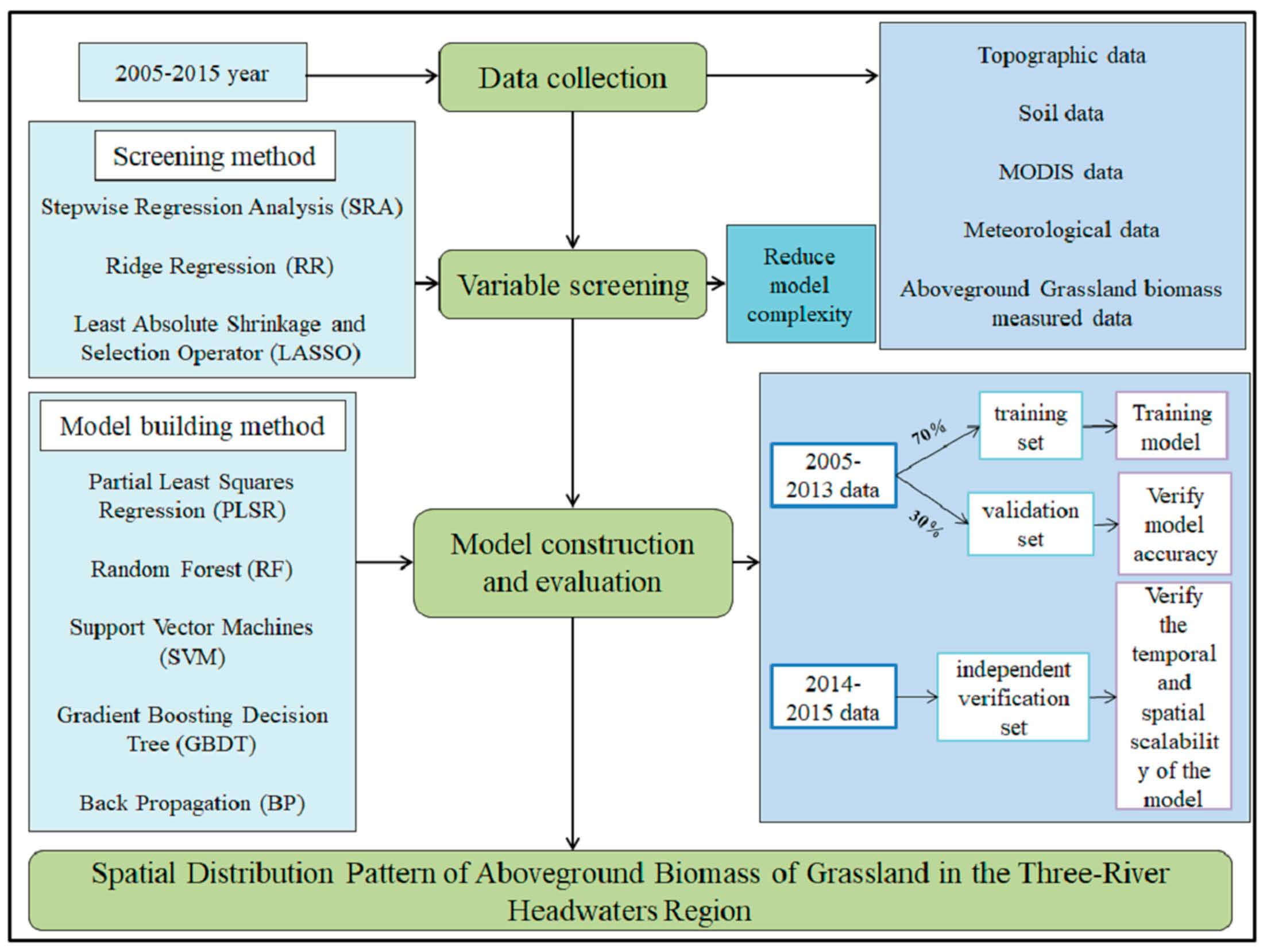
2. Data Sources and Methods

2.1. Data Sources

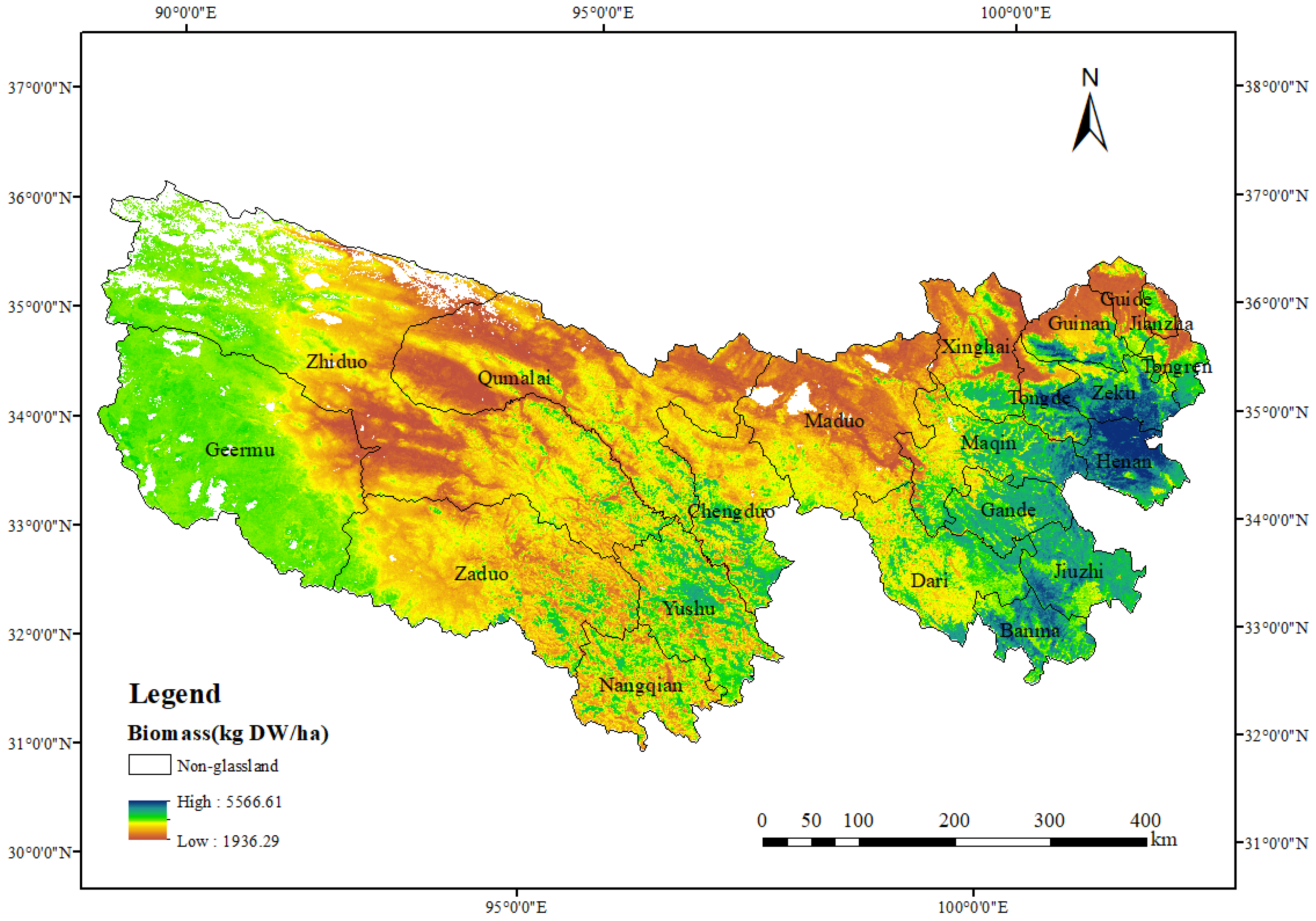
2.1.1. Study Area

The study area (31°39′~36°12′N, 89°45′~102°23′E) is located in the southern part of Qinghai Province in China. It is the ecological barrier between the roofs of the world (the Qinghai Tibet Plateau) and is the headwater source of the three largest rivers in China: the Yellow River, the Yangtze River, and the Lancang River. The TRHR is known as the China Water Tower and provides a barrier for environmental protection and sustainable development for the middle and lower reaches of rivers in China and Southeast Asian countries. The study area has a total area of 36,561,502 ha, accounting for about 43% of the total area of Qinghai Province. The average altitude is 4000 m, the annual mean temperature (AMT) is 3 °C, the annual mean precipitation (AMP) is 377 mm, and its range of growing degree days (GDDs) is 0–5001 °C. The grassland in the TRHR is dominated by alpine meadows and alpine grasslands, accounting for 54% and 16% of the area, respectively (Figure 1b). The soil distribution in the area has prominent vertical zoning rules, mainly alpine meadow soil and swamp meadow soil, and the frozen soil layer is well developed [22]. Details of research sites are supplemented in the Table S1.

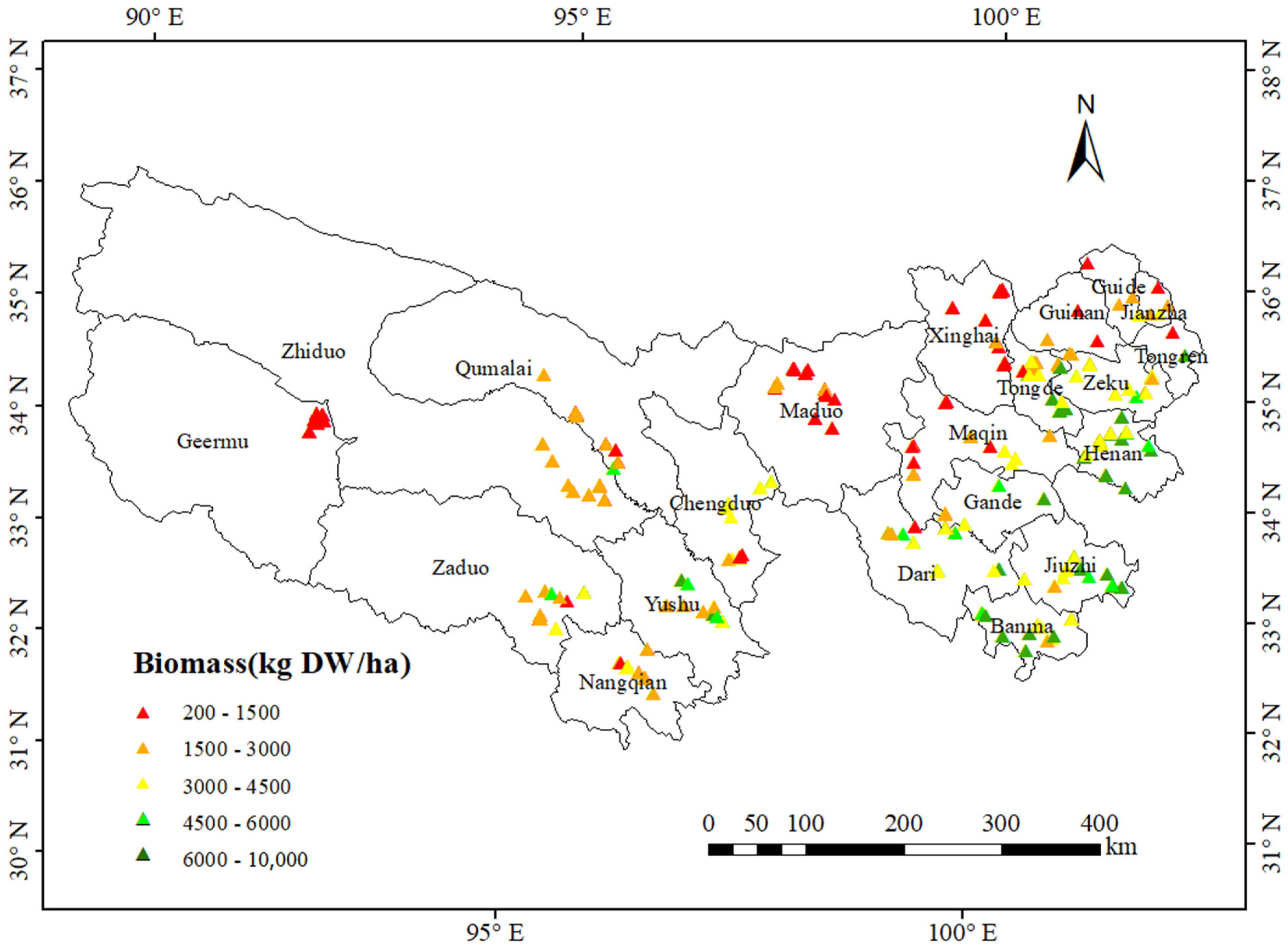
2.1.2. AGB Dataset

We collected field survey AGB data during the peak growing season (July to September) from 2005 to 2015, for a total of 1620 valid data items (Table S2). Guide, Guinan, Jianzha, and Tongren were newly added in 2015, and each county has only 2 to 5 sample points. The largest number of samples was of those drawn from Banma county, with 120 sample points collected, followed by Tongde county, with 115 sample points collected.

The general spatial distribution of AGB measurements during 2005–2015 provides an overall picture of the AGB values of the study area (Figure 2). As shown in the figure, the value of AGB was in the range from 200 to 10,000 kg DW (dry matter weight)/ha (the average value was 3090 kg DW/ha). The figure shows an overall downward trend from southeast to northwest, with some exceptions.

We now outline the methodological steps undertaken to collect the grassland AGB of the study (Figure S1).

a)

The latitude and longitude of the TRHR were determined by a handheld GPS device.

b)

We established a grassland sample plot (500 m × 500 m) based on typical grassland vegetation communities that had a relatively flat terrain and uniform growth and that were spatially representative. We used five 1 m × 1 m grassland observation plots in the sample plot using the five point method.

c)

The aboveground part of the vegetation in each observation plot was mowed up to the ground. All litter and other non-plant materials were removed from the grass samples, bagged, and brought back to the laboratory for further processing.

d)

We weighed samples from each plot in the laboratory. They were then oven-dried at 65 °C for 48 h, and their dry weights were recorded.

All AGB values (dry weight) in a MODIS pixel (500 × 500 m) were averaged to represent the average AGB of the MODIS pixels, and the center latitude and longitude of the pixel were used for modeling.

2.1.3. Meteorological Data

Climatic data as an environmental factor are the basis of research fields such as agriculture and forestry. We collected the daily maximum temperature, minimum temperature, and precipitation data from 15 meteorological stations in the TRHR from 2005 to 2015 from the China Meteorological Data Network (http://data.cma.cn, accessed on 3 February 2021). AMT and AMP were interpolated by ANUSPLIN, an interpolation package specially designed for meteorological data [23].

2.1.4. Soil Data and Topographic Data

The soil data were from the global gridded soil information (https://soilgrids.org/, accessed on 3 February 2021) and included the organic carbon stock of soil (OC) on the surface (0–5 cm), organic carbon density (OR) on the surface (0–5 cm), bulk density (BL) of the soil surface (0–5 cm), (CL) of the soil surface (0–5 cm), coarse fragments (CR) (0–5 cm), silt size (SL) of the soil surface (0–5 cm), sand (SN) on the soil surface (0–5 cm), cation exchange capacity (at pH = 7) (CE) of the soil surface (0–5 cm), and pH water (pH) in the soil surface (0–5 cm). We then resampled the data to 500 m.

The digital elevation model (DEM) data were obtained from Shuttle Radar Topography Mission (SRTM) images (version 004) (http://srtm.csi.cgiar.org, accessed on 3 February 2021). To match the available data, the digital elevation data were resampled to 500 m, and the projection type was defined as a WGS_1984 map projection. In addition, ArcGIS software was used to generate the aspect and slope with a resolution of 90 m; the data were then resampled to 500 m. Finally, we extracted the corresponding data and analyzed them.

2.1.5. MODIS Data and Its Processing

All MODIS data in this paper were obtained from the Google Earth Engine (GEE) platform (https://code.earthengine.google.com/, accessed on 7 February 2021) (version 006) (

Table 1. MODIS products.

MODIS	Time Resolution (d)	Spatial Resolution (m)	Bands
MOD09A1	8	500	B1–B7
MOD13A1	16	500	NDVI, EVI
MOD11A2	8	1000	D-LST, N-LST
MOD15A2H	8	500	LAI, Fpar

Note: B1–B7: reflectance of MODIS bands 1–7; NDVI: normalized difference vegetative index; EVI: enhanced vegetation index; the unit of the day land surface temperature (D-LST) and night land surface temperature (N-LST) is K; LAI: leaf area index; Fpar: fraction of photosynthetically active radiation.

and Table S3). The processing flowchart is shown in Figure S2.

2.2. Method and Modeling

2.2.1. Variable Selection

Three variable selection methods, stepwise regression analysis (SRA), ridge regression (RR), and the least absolute shrinkage and selection operator (LASSO), were used in this study. As a filter of variable indicators, SRA can quickly select the most important variable indicators related to the research object from a large number of indicator libraries [24]. RR is a variable screening method and has the ability to handle multicollinearity data [25]. LASSO can automatically select the most important independent variables and narrow down the less important predictor variables to zero [26].

2.2.2. Summary of Modeling Methods

The PLS, SVM, RF, Gradient Boosting Decision Trees (GBDT), and Multilayer BP Neural Network (BP) modeling methods were used. The PLS is a mathematical regression model that determines the correlation between variables [27]. The two most important parameters in the RF algorithm are the number of regression trees and the number of predictors at each node. When the number of regression trees is set larger, the accuracy of the model will also be improved, but the model operation time will be prolonged. The default value of the number of predictors at each node is 1/3 of the total number of independent variables [28]. The SVM is a type of machine learning theory based on statistical learning theory [29]. In this paper, the radial basis function was used as the kernel function, and the genetic algorithm was used to optimize two key parameters (gamma and cost). These three algorithms use functions from the R packages “PLSR”, “random forest”, and “e1071.” GBDT is an integrated model based on a decision tree that contains flexible and efficient machine learning algorithms [30]. We continuously optimized the three hyperparameters of the learning rate, the number of iterations, and the subsample. The GBDT method was implemented based on the gradient boosting regressor in the sklearn package. BP is a multi-layer forward neural network, and its theoretical basis is the error direction propagation algorithm [31]. The most important parameters in the BP model are the number of neurons and hidden layers, which need to be repeatedly tested and continuously tuned. The BP model is built based on the torch deep learning framework. The rationale for machine learning algorithms was added to the Supplementary Materials (Text S1).

2.2.3. Assessing Model Accuracy

The square of the correlation coefficient between the measured value on the ground and the predicted value of the model (R²) and root mean square error (RMSE) values were used as the standards of accuracy evaluation. Higher R² and lower RMSE indicate better model performance. Equations (1) and (2) express R² and RMSE respectively:

$${\mathrm{R}}^2=1-\frac{{{\displaystyle \sum }}_{\mathrm{i}=1}^{\mathrm{n}}{\left(\mathrm{Yi}-\widehat{\mathrm{Yi}}\right)}^2}{{{\displaystyle \sum }}_{\mathrm{i}=1}^{\mathrm{n}}{\left(\mathrm{Yi}-\overline{\mathrm{Yi}}\right)}^2}$$

(1)

$$\mathrm{RMSE}=\sqrt{\frac{{{\displaystyle \sum }}_{\mathrm{i}=1}^{\mathrm{n}}{\left(\mathrm{Yi}-\widehat{\mathrm{Yi}}\right)}^2}{\mathrm{n}}}$$

(2)

where Yi represents the measured value of the aboveground biomass of grassland, $\widehat{\mathrm{Yi}}$ is the predicted value of Yi, and $\overline{\mathrm{Yi}}$ is its average value.

The model selection process took into account its fitting performance and simplicity. In this study, AIC and BIC were used as the evaluation criteria. Among the models with the same fitting ability, the model with the smaller BIC was preferred.

Equations (3) and (4) express AIC and BIC respectively:

$$\mathrm{AIC}=\mathrm{k}\ln \left(\mathrm{n}\right)+\mathrm{n}\ln \left(\frac{{{\displaystyle \sum }}_{\mathrm{i}=1}^{\mathrm{n}}{\left(\mathrm{Yi}-\widehat{\mathrm{Yi}}\right)}^2}{\mathrm{n}}\right)$$

(3)

$$\mathrm{BIC}=2\mathrm{k}+\mathrm{n}\ln \left(\frac{{{\displaystyle \sum }}_{\mathrm{i}=1}^{\mathrm{n}}{\left(\mathrm{Yi}-\widehat{\mathrm{Yi}}\right)}^2}{\mathrm{n}}\right)$$

(4)

where Yi represents the measured value of the aboveground biomass of grassland, $\widehat{\mathrm{Yi}}$ is the predicted value of Yi, k represents the number of variables in the model, and n represents the number of samples. The larger the R², the higher the credibility of the model prediction, the smaller the RMSE, AIC, and BIC, the better the model fitting effect.

3. Results

3.1. Correlation between Grassland AGB and Variables

This study used the correlation analysis method to test the correlation between AGB and MODIS data, topographical factors, soil factors, and meteorological factors (Table S4). As shown in the table, there was a significant correlation between the AGB and most MODIS vegetation indices. Among them, grassland AGB had the highest positive correlation coefficient with the NDVI, MSAVI, optimized soil-adjusted vegetation index (OSAVI), and SAVI (R = 0.51). The correlation coefficient between AGB and the reflectance of the MODIS bands (B1–B7) was between −0.44 and 0.39. The correlation with B7 was the largest (R = −0.44). There was a strong correlation between the aboveground biomass of grassland and the five band indices (C–G). Among them, AGB had the largest correlation with E.

The AGB was significantly correlated with most variables, and only had a weak relationship with topographical factors and SL among soil factors (R < 0.1). AGB and slope had the highest correlation coefficient (R = 0.29), followed by the DEM, and the weakest relationship was with the aspect. The BLD, SN, and pH were negatively correlated with the AGB, but the AGB had a positive correlation with the other soil factors, among which, the relationship with CL was the strongest (R = 0.26). Among the meteorological factors, AGB had a significant relationship with AMT, GDD, and AMP, but only showed a negative correlation with GDD.

3.2. Variable Screening and Model Evaluation

We divided the variables into the All set (45 variables), SRA subset (12 variables), RR subset (11 variables), and LASSO subset (17 variables) (

Table 2. Results of variables screening by different screening methods.

Methods	Variable Set	Filter Number
ALL	DEM Slope Aspect BLD CEC CL SN SL pH OR OC CR B1-B7 C D E F G BI DVI EVI Fpar LAI MSAVI NDSI NDVGI NDVI NDWI OSAVI RVI SATVI SAVI SCI TVI D-LST N-LST AMT GDD AMP	45
SRA	DEM CL pH OR OC B1 B5 B6 OSAVI D-LST N-LST GDD	12
RR	DEM SN SL pH OC B3 B5 B6 BI D-LST GDD	11
LASSO	DEM Slope CL SN pH B2 B6 C E EVI LAI MSAVI NDVGI OSAVI AMT GDD AMP	17

Note: DEM: digital elevation model; BLD: bulk density; CEC: cation exchange capacity (at pH = 7); CL: clay content; SN: sand; SL: silt size; OR: organic carbon density; OC: soil organic carbon stock; CR: coarse fragments; B1–B7: the reflectance of the MODIS bands 1–7; C–G: five band indices (Band 2–7 (C), Band 5/Band 2 (D), (Band 5 − Band 7)/(Band 5 + Band 7) (E), Band 7/Band 2 (F), and Band 7/Band 5 (G)); BI: brightness index; DVI: difference vegetation index; EVI: enhanced vegetation index; Fpar: fraction of photosynthetically active radiation; LAI: leaf area index; MSAVI: modified soil-adjusted vegetation index; NDSI: normalized difference soil index; NDVGI: normalized difference vegetation green index; NDVI: normalized difference vegetative index; NDWI: normalized difference water index; OSAVI: optimized soil-adjusted vegetation index; RVI: ratio vegetation index; SATVI: soil-adjusted total vegetation index; SAVI: soil-adjusted vegetation index; SCI: soil color index; TVI: transformed vegetation index; D-LST: day land surface temperature; N-LST: night land surface temperature; AMT: annual mean temperature; GDD: growing degree days; AMP: annual mean precipitation.

). We used these variable sets as input variables and respectively constructed the PLS, RF, SVM, GBDT, BP models, for a total of 20 models. The accuracy of the predicted aboveground biomass of each model in the TRHR was assessed (

Table 3. Assessment of accuracy of the multi-factor grassland AGB estimation model.

		Training Dataset		Testing Dataset		Independent Testing Dataset		AIC	BIC
Variable Set	Model	R2	RMSE	R2	RMSE	R2	RMSE
ALL	PLS	0.38	1459.00	0.45	1431.62	0.34	1487.92	5757.92	5936.40
	RF	0.92	620.99	0.59	1253.24	0.43	1396.90	5654.12	5832.59
	SVM	0.73	1037.59	0.55	1342.84	0.41	1492.87	5707.99	5886.46
	GBDT	0.85	766.67	0.59	1239.59	0.38	1460.16	5645.58	5824.06
	BP	0.94	460.09	0.50	1427.26	0.34	1614.86	5755.54	5934.01
SRA	PLS	0.36	1484.46	0.49	1385.01	0.36	1474.83	5666.10	5713.70
	RF	0.91	664.34	0.60	1245.85	0.50	1332.59	5583.51	5631.10
	SVM	0.51	1336.17	0.54	1365.37	0.39	1490.64	5654.96	5702.56
	GBDT	0.77	931.60	0.56	1288.12	0.38	1447.90	5609.53	5657.13
	BP	0.69	1054.13	0.53	1359.04	0.30	1612.39	5651.34	5698.93
RR	PLS	0.35	1493.14	0.50	1382.86	0.35	1477.88	5662.89	5706.52
	RF	0.90	682.57	0.58	1271.56	0.46	1363.59	5597.44	5641.07
	SVM	0.48	1362.57	0.50	1399.81	0.41	1479.49	5672.39	5716.02
	GBDT	0.77	929.48	0.57	1275.69	0.41	1418.99	5599.97	5643.60
	BP	0.58	1204.95	0.49	1407.71	0.34	1515.10	5676.78	5720.41
LASSO	PLS	0.35	1499.63	0.48	1406.04	0.36	1480.31	5687.86	5755.28
	RF	0.91	657.03	0.58	1263.89	0.45	1378.47	5604.72	5672.15
	SVM	0.58	1258.28	0.55	1354.10	0.36	1503.76	5658.50	5725.92
	GBDT	0.70	1050.85	0.57	1272.33	0.41	1408.85	5609.91	5677.33
	BP	0.74	963.93	0.46	1457.26	0.26	1663.55	5715.77	5783.19

Note: SRA: stepwise regression analysis; RR: ridge regression; LASSO: least absolute shrinkage and selection operator; PLS: partial least squares; RF: random forest; SVM: support vector machine; GBDT: gradient boosting decision tree; BP: multi-layer back-propagation neural network.

). The results show the following:

(1)

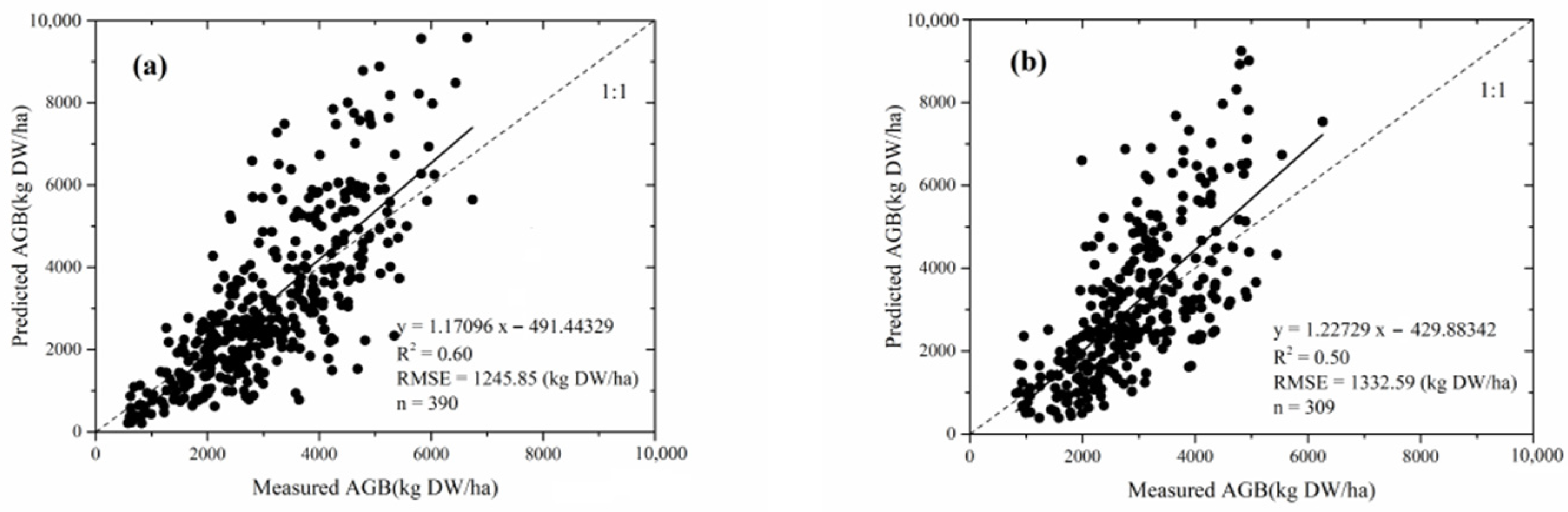
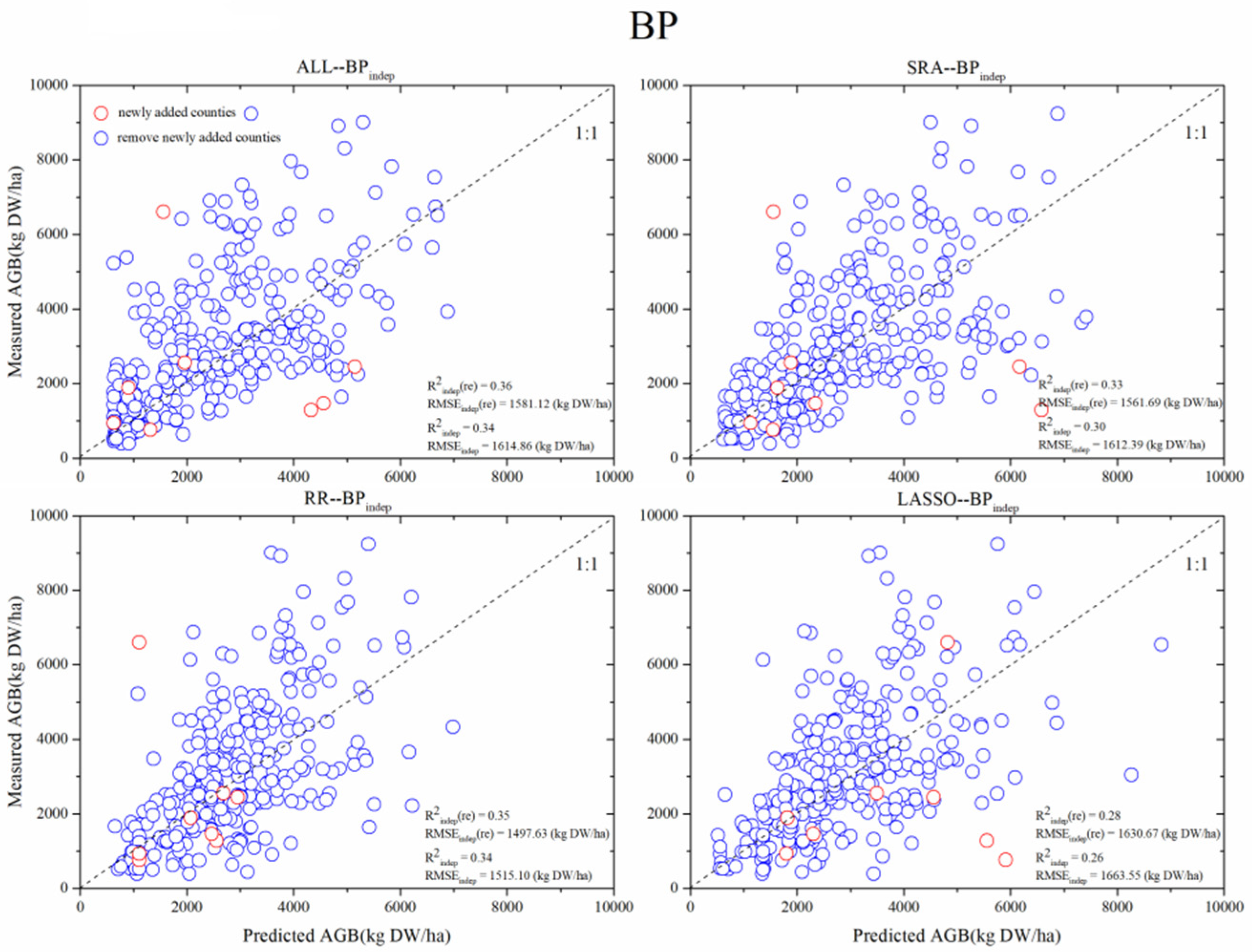
Overall, the R² of the training set (R²_train) of the 20 models was between 0.35 and 0.94, with an average of 0.67, and the RMSE of the training set (RMSE_train) was between 460.09 and 1499.63 kg DW/ha, with an average of 1045.87 kg DW/ha. The R² of the validation set (R²_vad) was between 0.45 and 0.6, with an average of 0.53, and the RMSE of the validation set (RMSE_vad) was between 1239.59 and 1457.26 kg DW/ha, with an average of 1341.46 kg DW/ha. The R² of the independent verification set (R²_indep) was between 0.26 and 0.50, with an average of 0.38, and the RMSE of the independent verification set (RMSE_indep) was between 1332.59 and 1663.55 kg DW/ha, and the average was 1475.05 kg DW/ha. The AIC of the independent verification set was between 5583.51 and 5757.92, and the BIC of the independent verification set was between 5631.1 and 5936.4. The SRA-RF model had the largest R²_vad and R²_indep, the smallest RMSE_vad, RMSE_indep, AIC, and BIC, and the best predictions (RF-R²_vad = 0.60, RF-RMSE_vad = 1245.85 kgDW/ha, RF-R²_indep = 0.50, RF-RMSE_indep = 1332.59 kg DW/ha, RF-AIC = 5583.51, RF-BIC = 5631.1). The RF model based on SRA achieved more accurate prediction results with a small number of variables, so the RF-SRA (RF-R²_vad = 0.60 (Figure 3a); RF-R²_indep = 0.50 (Figure 3b)) was the best model.

(2)

During the selection of variables, the DEM among terrain-related factors, the pH among soil-related factors, the B6 among remote sensing-related factors, and the GDD among meteorological factors were selected. These four variables had significant effects on the grassland biomass.

(3)

Although the overall fitting performance of the estimation model based on the RF method (the average of RF-R²_train was 0.91) was much higher than that based on the PLS method (the average of PLS-R²_train was 0.36)), its predictive performance (RF-R²_vad was between 0.58 and 0.6, and the average was 0.59) was not (RF-R²_vad was between 0.45 and 0.50, and the average was 0.48).

(4)

Judging from the prediction results of the model, among the results based on different variables, the results of the RF algorithm were superior to the other algorithms; the model had a higher R² and a lower RMSE (RF-All-R²_vad = 0.59, RF-SRA-R²_vad = 0.60, RF-RR-R²_vad = 0.58, and RF-LASSO-R²_vad = 0.58).

(5)

Overall, the R²_vad (between 0.45 and 0.6 and the average value of 0.53) and RMSE_vad (the average value was 1341.46 kg DW/ha) of the 20 models’ test sets were superior to R²_indep (between 0.26 and 0.5, the average value was 0.38) and RMSE_indep (the average value was 1475.05 kg DW/ha). Of the 20 models, 12 AGB models had values of R²_vad greater than or equal to the average R²_vad (R² = 0.53) of all models. This shows that at least 60% of the 20 models had a high accuracy and that these models can reflect 53–60% of the changes in the grassland AGB. Of the 20 models, 11 AGB models had an R²_indep greater than or equal to the average R²_indep (0.38) of all models, which shows that, when these models were expanded in time and space, their predictive ability declined. Of the 20 models, at least 56% reflected 38–50% of the changes in AGB in the next two years and over more space in the TRHR.

(6)

We found that the model was optimal for the following combinations: (1) RF, SVM, BP, and SRA; (2) PLS, GBDT, and RR; and the model’s spatio-temporal scalability was optimal for the following combinations: (3) PLS, RF, and SRA, (4) SVM, BP, and RR, (5) GBDT and LASSO. The All set had the worst performance of the models for grassland aboveground bio-mass, and variable selection helped improve model accuracy.

The relationship between the number of sampling points and the accuracy of the model is shown in Figure 4. In general, the RF algorithm delivered the best performance, with a value of R² that was higher than the other algorithms. The simulation accuracy of the model changed drastically with the number of samples. We take the RF-SRA model as an example. The R²_vad of the RF-SRA model was between 0.52 and 0.74, with a difference of 0.22. The slope of the trend line about the RF-SRA model was −0.0231. The R²_indep of the RF-SRA model was between 0.4 and 0.5, with a difference of 0.1.

In Figure 4 the ordinate represents R², and the abscissa represents the sample size (30% (390 data items) meaning that 30% of all samples in 2005–2013 were randomly selected for three to seven points and were then modeled and verified); 40% means that 517 data items were used, 50% means 650 items, 60% means 794 items, 70% means 921 items, 80% means 1042 items, 90% means 1178 items, and 100% means 1311 items.

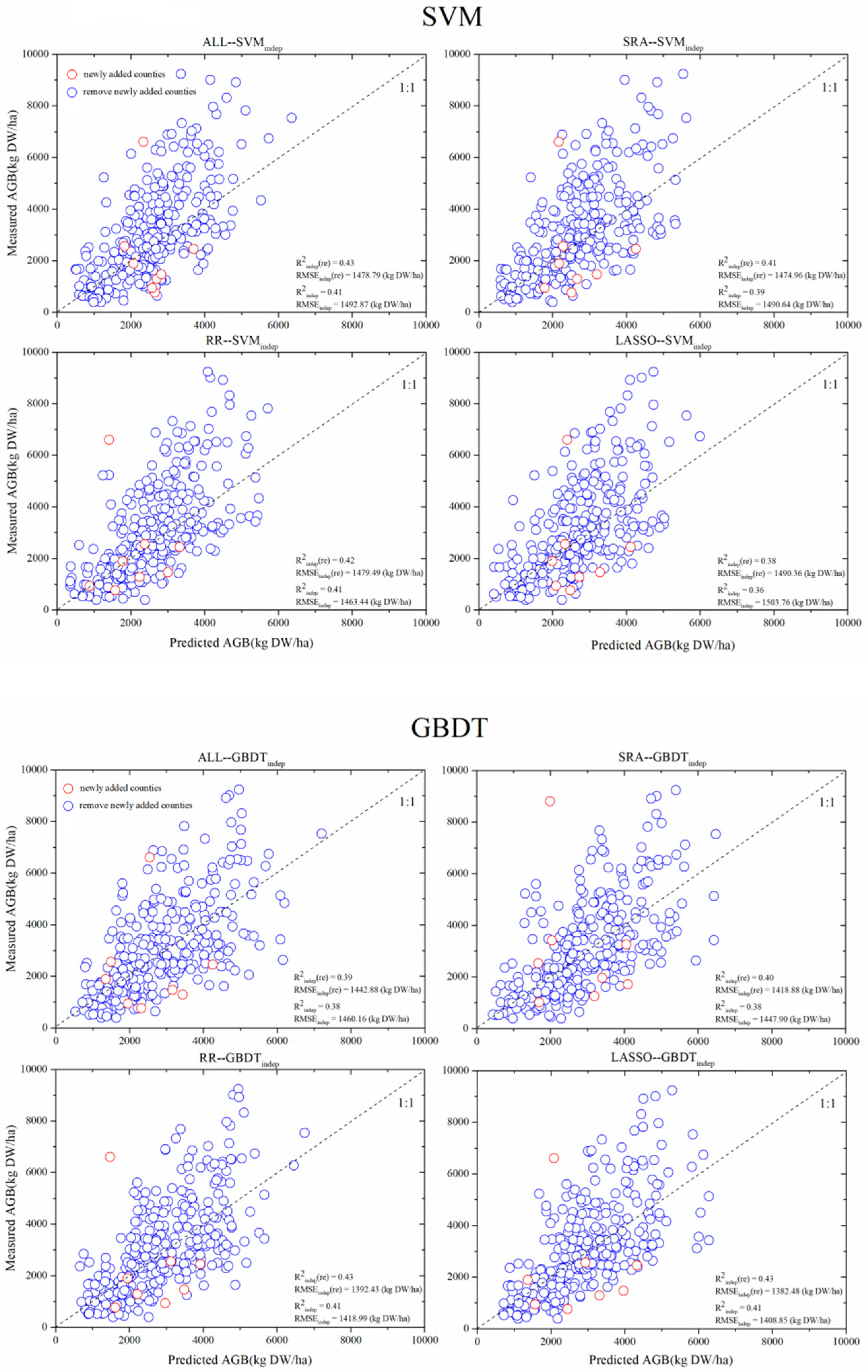
3.3. Assessing Spatial and Temporal Sample Distributions

When the five models were expanded in space and time, their accuracy decreased (the average R² of the 20 models decreased by 0.15 (Table 3). We bring the results (R²_indep, RMSE_indep) of the independent testing dataset in Table 3 into Figure 5 for further exploration. In Figure 5, the red dots represent the AGB of the newly added locations from 2014 to 2015, the blue dots represent those of no newly added locations from 2014 to 2015, that is, “re”. Comparing the R²_indep, RMSE_indep (the model with the independent validation set as the test set) and R²_indep (re), RMSE_indep (re) (the model with data that only scales in the temporal direction as the test set), the results show that the accuracy of adding new points (R²_indep) was lower than that of not adding new points (R²_indep (re)), which indicates that adding new points reduced accuracy. That is, when the model was extended in space, its accuracy decreased (models calibrated at small scales, when transferred to large scales, incur errors).

3.4. Spatial Distribution and Trend of Grassland Biomass Based on the RF-SRA Model

The RF-SRA model (the best model in this study) was used to simulate the annual maximum grassland aboveground biomass (the maximum aboveground biomass from July to September) in the study area for 11 years (2005 to 2015). Figure 6 illustrates the average results of the annual maximum grassland AGB in these 11 years (the average maximum AGB in the TRHR from 2005 to 2015 was 3267.41 ± 651.34 kg DW/ha). The results show that the higher grassland AGB was mainly concentrated in the eastern part of the study area and some of its western parts. For instance, Zaduo, Zhiduo, Qumalai, Maduo, and Northern Xinghai had lower distributions of grassland AGB. However, areas such as Xinghai, Guinan, and Guide also had lower altitudes and less AGB.

4. Discussion

4.1. AGB Mapping

In general, based on the inversion of the optimal model (RF-SRA), the annual spatial distribution of the largest grassland AGB showed an increasing trend from west to east and from north to south (Figure 6). This may be because the eastern region is a major pastoral area, with a higher temperature, a higher altitude, and a colder climate in the west of the TRHR (Figure 1). However, areas such as Xinghai, Guinan, and Guide have lower altitudes and less AGB, possibly due to a higher population density and more frequent human activities [32]. The generalized spatial distribution of AGB measurements during 2005–2015 provides an overall picture of the AGB values of the study area: an overall downward trend from southeast to northwest on the whole (Figure 2). This is consistent with the spatial variation of annual precipitation in the aboveground biomass of grassland [32]. At the same time, the annual average temperature gradually increased from west to east and was related to the trend of change in the longitude [33]. Precipitation and the annual mean temperature were positively correlated with grassland coverage in the Three-River Headwaters (Table S4). The spatial variation in grassland cover in this region may be influenced by both precipitation and annual temperature. The estimated spatial distribution map of AGB based on the RF models showed a reasonable spatial distribution, similar to that reflected in on-site measurements. A digital map can provide more details and cover a larger space than a limited field measurement (even though more than 1000 samples were collected).

4.2. Factors Affecting the Accuracy of the Remote Sensing Grassland AGB Estimation Model

Although the RF-SRA model attained accurate predictions, we think that its accuracy can be further improved. We analyze factors that affected the accuracy of the model:

(1)

There were inevitable temporal differences between the biophysical parameters measured in the field and the satellite data during the peak growth period of the grasslands [34]. The field sampling time cannot be exactly the same as the time corresponding to the maximum vegetation index obtained from satellite data. In addition, the time period of this study was from 2005 to 2015. The first Sentinel-1 satellite was launched in 2014, so the Sentinel data of our study time are not available. TRHR is located in the hinterland of the Qinghai-Tibet Plateau. The high altitude and variable climate mean that it is often covered by clouds, which in turn leads to unusable Landsat data, that is, a lack of long-term continuous Landsat observation data. To obtain more variables and consider such practical difficulties as data availability within the study period, we selected MODIS data with a resolution of 500 × 500 m. However, in practice, the field sampling points are relatively small in number, and each pixel in the MODIS data covers an area of 500 × 500 m. Therefore, some differences were obtained in the spatial representation. In future work, more accurate and higher-resolution remote sensing data can be used, such as those obtained using unmanned aerial vehicles, to improve accuracy.

(2)

Areas with complex terrain and slopes impacted reflectivity, which in turn affected the accuracy of the model. In addition, generally sparse grasslands (bare soil points) also affected some vegetation indices (such as the NDVI), which ultimately affected the model [35]. The grassland biomass measurements in this study were mainly distributed in the central and eastern regions of the TRHR. Grasslands in the western part of the TRHR are very sparse; many areas are deserts (Figure 1b). In addition, the western region has a higher altitude, a colder climate, and more complex terrain, which also introduced difficulties in sampling. We thus collected few and very concentrated samples in the western part of TRHR (only AGB data in the northeast of Geermu). This further affected the accuracy of the model.

(3)

Uncertainty in field measurements also affected the model. For example, in-field measurements, the data collected are often affected by surface heterogeneity, human factors, and even traffic conditions. The data in this study cover a large span of time, and there is a large amount of it. A time span that is too long and an amount of data that is too high can also lead to more errors in data measurement during the sorting process, which will inevitably affect the construction of the model.

4.3. Influence of the Number of Field Samples on the Model and the Model’s Spatio-Temporal Scalability

The precision of AGB inversion models is highly dependent on the number of field samples. However, most studies have used fewer than 1000 field samples [17]. We measured continuous values of the grassland biomass in the TRHR for 11 years (1620 field samples) to explore the relationship between the field samples and the model. When constructing the AGB model, large differences were obtained in the structure and parameters of the model with the number of the field samples, and the accuracy of the simulation changed as well. Therefore, to better represent grasslands, more data points should be collected when sampling.

Previous studies have demonstrated that validation is key in this context. Without proper validation or a mechanistic understanding of the model, it is difficult to assess the quality of the results. Few studies have sought to estimate the validation error in AGB using ML [17]. AGB has traditionally been measured by destructive methods, which are limited to small areas due to their nature, time, expense, and the labor involved [36]. Therefore, evaluating the usefulness of the algorithm is important [37]. We used four criteria to evaluate the model. Figure 5 shows the results detailed in Table 3. Combining the graph and table comparison, it was found that model accuracy decreased when it was applied to the years without training data. When the model expands to an area with field sampling points that have not been incorporated into the model training, the model’s accuracy will further decrease (Figure 5).

4.4. Input Variables to the Model

Environmental factors are important factors in determining the types, characteristics, and distribution of grasslands. Cui et al. (2015) found that the biomass of alpine grassland decreases with the increase of altitude. In this study, AGB showed a negative correlation with DEM (Table S4), which was the same as their findings [38]. However, the relationship between AGB and DEM in this paper is weak, which may be because the study did not set a certain altitude gradient when collecting points in the field. Moreover, when the samples were set, the research was mostly carried out on relatively flat grassland, which may also be the reason for the weak relationship between AGB and Aspect and Slope.

Soil is mainly composed of mineral particles, which can be divided into CL, SL, and SN according to their thickness. AGB was positively correlated with CL and negatively correlated with SN. Su et al. found that soils with higher CL usually have higher soil organic carbon, nutrient content and higher cation exchange capacity, and higher nutrient retention capacity and water holding effect to promote the growth of grassland vegetation [39]. The soil with higher SN has poor water holding effect, which is not conducive to the growth of vegetation. This is consistent with our results. AGB is negatively correlated with pH. The possible reason is that the pH of the study area is between 5.4 and 7.7. In the acidic soil, the species of microorganisms are limited and the decomposition of organic matter is slowed down, and the microbial activity is high in the neutral or alkaline environment [40], which is conducive to vegetation growth.

Among climatic factors, both AMP and AMT were positively correlated with AGB (Tables S4 and S5 and Figure S3, which may be because the increase of AMP and AMT promoted the growth of grassland vegetation. In the random forest importance ranking, GDD ranks second (Figure S4, and there is a negative correlation between GDD and AGB, which may be because the increase in GDD leads to faster plant development, but the actual growth season is shortened, resulting in a decrease in grassland AGB.

Satellite remote sensing is currently the most common and widely used regional-scale surface detection method. Satellite data can directly and timely capture biological growth status through various spectral bands, and the products of various satellites have the same or complementary biological information, which is beneficial to grassland biomass prediction [5]. Different vegetation indices can reflect different biological characteristics of crops. For example, SAVI can indirectly reflect the canopy temperature of crops and reduce the influence of soil background on canopy reflectance [41]. In this study, OSAVI was the most important for the model (Figure S4. The OSAVI vegetation index is a modified SAVI, which differs from SAVI in that OSAVI takes into account the standard value of the canopy background adjustment factor (0.16). Therefore, when the canopy cover is low, this adjustment allows greater soil variation for OSAVI compared to SAVI. Therefore, higher predictability can be obtained.

5. Conclusions

Our study integrated 1620 measurement data on aboveground grassland biomass (AGB) with corresponding, continuously monitored remote sensing data from the GEE platform, meteorological data, topographic data, and soil characteristic data collected over 11 years in the TRHR of China. We then used the linear statistical method (PLS), ML methods (RF, SVM, and GBDT), and DL methods (BP) to establish grassland AGB estimation models. We then compared the models in terms of the accuracy of biomass predictions and simplicity. We also explored the spatio-temporal scalability of the linear regression model and the machine learning models. Overall, the ML models performed well. The RF models, based on the DEM, CL, pH, OR, OC, B1, B5, B6, OSAVI, D-LST, N-LST, and GDD, delivered the best performance. The estimated spatial distribution map of AGB based on the RF models was reasonably similar to the distribution of on-site measurements. It also provided more detail and covered a larger space than the limited field measurements do (even though more than 1000 samples were collected). This shows that when models are expanded in space and time, their accuracy decreases (as an example, the accuracy of the SRA-RF model decreased from 0.6 to 0.5). In future research, a process-based model that is derived from grassland AGB to train models could potentially be used to extend the spatio-temporal scalability of machine learning models. In addition, we also believe that ecosystem carbon sequestration is an interesting topic. In future work, we intend to explore whether the optimal model has the potential to be used in the development of emission factors for grassland areas from the perspective of addressing global climate change and combining the results of this study.

References

- Yang, Q.; Liu, G.; Giannetti, B.F.; Agostinho, F.; MVBAlmeida, C.; Casazza, M. Emergy-based ecosystem services valuation and classification management applied to China’s grasslands. Ecosyst. Serv. 2020, 42, 101073. [Google Scholar] [CrossRef]
- Hensgen, F.; Bühle, L.; Wachendorf, M. The effect of harvest, mulching and low-dose fertilization of liquid digestate on above ground biomass yield and diversity of lower mountain semi-natural grasslands. Agric. Ecosyst. Environ. 2016, 216, 283–292. [Google Scholar] [CrossRef]
- Zhou, W.; Li, H.; Xie, L.; Nie, X.; Wang, Z.; Du, Z.; Yue, T. Remote sensing inversion of grassland aboveground bio-mass based on high accuracy surface modeling. Ecol. Indic. 2021, 121, 107215. [Google Scholar] [CrossRef]
- Wang, Z.B.; Ma, Y.K.; Zhang, Y.N.; Shang, J.L. Review of Remote Sensing Applications in Grassland Monitoring. Remote Sens. 2022, 14, 2903. [Google Scholar] [CrossRef]
- Guan, K.; Wu, J.; Kimball, J.S.; Anderson, M.C.; Frolking, S.; Li, B.; Hain, C.R.; Lobell, D.B. The shared and unique values of optical, fluorescence, thermal and microwave satellite data for estimating large-scale crop yields. Remote Sens. Environ. 2017, 199, 333–349. [Google Scholar] [CrossRef] [Green Version]
- Erica, G.; Andrew, H.; Rick, L. Using NDVI and EVI to Map Spatiotemporal Variation in the Biomass and Quality of Forage for Migratory Elk in the Greater Yellowstone Ecosystem. Remote Sens. 2016, 8, 404. [Google Scholar]
- Gilabert, M.A.; González-Piqueras, J.; Garca-Haro, F.J.; Meliá, J. A generalized soil-adjusted vegetation index. Remote Sens. Environ. 2002, 82, 303–310. [Google Scholar] [CrossRef]
- Ren, H.; Zhou, G.; Zhang, F. Using negative soil adjustment factor in soil-adjusted vegetation index (SAVI) for above-ground living biomass estimation in arid grasslands. Remote Sens. Environ. 2018, 209, 439–445. [Google Scholar] [CrossRef]
- Qi, J.; Chehbouni, A.; Huete, A.R.; Kerr, Y.H.; Sorooshian, S. A modified soil adjusted vegetation index. Remote Sens. Environ. 1994, 48, 119–126. [Google Scholar] [CrossRef]
- Guerschman, J.P.; Hill, M.J.; Renzullo, L.J.; Barrett, D.J.; Marks, A.S.; Botha, E.J. Estimating fractional cover of photosynthetic vegetation, non-photosynthetic vegetation and bare soil in the Australian tropical savanna region upscaling the EO-1 Hyperion and MODIS sensors. Remote Sens. Environ. 2009, 113, 928–945. [Google Scholar] [CrossRef]
- Lobell, D.B.; Thau, D.; Seifert, C.; Engle, E.; Little, B. A scalable satellite-based crop yield mapper. Remote Sens. Environ. 2015, 164, 324–333. [Google Scholar] [CrossRef]
- Nakano, T.; Bat-Oyun, T.; Shinoda, M. Responses of palatable plants to climate and grazing in semi-arid grasslands of Mongolia. Glob. Ecol. Conserv. 2020, 24, e01231. [Google Scholar] [CrossRef]
- Wang, L.; Ali, A. Climate regulates the functional traits-aboveground biomass relationships at a community-level in forests: A global meta-analysis. Sci. Total Environ. 2020, 761, 143238. [Google Scholar] [CrossRef] [PubMed]
- Verrelst, J.; Camps-Valls, G.; Munoz-Mari, J.; Rivera, J.P.; Veroustraete, F.; Clevers, J.; Moreno, J. Optical remote sensing and the retrieval of terrestrial vegetation bio-geophysical properties–A review. Isprs J. Photo-Grammetry Remote Sens. 2015, 108, 273–290. [Google Scholar] [CrossRef]
- Tang, R.; Zhao, Y.T.; Lin, H.L. Spatio-Temporal Variation Characteristics of Aboveground Biomass in the Headwater of the Yellow River Based on Machine Learning. Remote Sens. 2021, 13, 3404. [Google Scholar] [CrossRef]
- Xie, Y.; Sha, Z.; Yu, M.; Bai, Y.; Zhang, L. A comparison of two models with Landsat data for estimating above ground grassland biomass in Inner Mongolia, China. Ecol. Model. 2009, 220, 1810–1818. [Google Scholar] [CrossRef]
- Morais, T.G.; Teixeira, R.F.M.; Figueiredo, M.; Domingos, T. The use of machine learning methods to estimate above-ground biomass of grasslands: A review. Ecol. Indic. 2021, 130, 108081. [Google Scholar] [CrossRef]
- Craine, J.M.; Nippert, J.B.; Elmore, A.J.; Skibbe, A.M.; Hutchinson, S.L.; Brunsell, N.A. Timing of climate variability and grassland productivity. Proc. Natl. Acad. Sci. USA 2012, 109, 3401–3405. [Google Scholar] [CrossRef] [Green Version]
- Liu, S.; Cheng, F.; Dong, S.; Zhao, H.; Hou, X.; Wu, X. Spatiotemporal dynamics of grassland aboveground biomass on the Qinghai-Tibet Plateau based on validated MODIS NDVI. Sci. Rep. 2017, 7, 4182. [Google Scholar] [CrossRef] [Green Version]
- Huete, A.; Didan, K.; Miura, T.; Rodriguez, E.; Gao, X.; Ferreira, L.G. Overview of the Radiometric and Biophysical Performance of the MODIS Vegetation Indices. Remote Sens. Environ. 2002, 83, 195–213. [Google Scholar] [CrossRef]
- Zhu, X.; Liu, D. Improving forest aboveground biomass estimation using seasonal Landsat NDVI time-series. Isprs J. Photogramm. Remote Sens. 2015, 102, 222–231. [Google Scholar] [CrossRef]
- Zhang, J.P.; Zhang, L.B.; Liu, W.L.; Qi, Y.; Wo, X. Livestock-carrying capacity and overgrazing status of alpine grass-land in the Three-River Headwaters region, China. Geogr. Sci. 2014, 24, 303–312. [Google Scholar] [CrossRef]
- Hutchinson, M.F. ANUSPLIN Version 4. 3 User Guide; The Australia National University, Center for Re-source and Environment Studies: Canberra, Australia, 2004; Available online: http://cres.anu.edu.au/outputs/anusplin.php (accessed on 13 February 2021).
- Chen, Y.; Shi, R.; Shu, S.; Gao, W. Ensemble and enhanced PM10 concentration forecast model based on stepwise regression and wavelet analysis. Atmos. Environ. 2013, 74, 346–359. [Google Scholar] [CrossRef]
- Dorugade, A.V. New ridge parameters for ridge regression. J. Assoc. Arab. Univ. Basic Appl. Sci. 2014, 15, 94–99. [Google Scholar] [CrossRef] [Green Version]
- Zhang, Y.; Ma, F.; Wang, Y. Forecasting crude oil prices with a large set of predictors: Can LASSO select powerful predictors? J. Empir. Financ. 2019, 54, 97–117. [Google Scholar] [CrossRef]
- Metz, M.; Abdelghafour, F.; Roger, J.; Lesnoff, M. A novel robust PLS regression method inspired from boosting prin-ciples: RoBoost-PLSR. Anal. Chim. Acta 2021, 1179, 338823. [Google Scholar] [CrossRef]
- Wang, Y.; Wu, G.; Deng, L.; Tang, Z.; Wang, K.; Sun, W.; Shangguan, Z. Prediction of aboveground grassland biomass on the Loess Plateau, China, using a random forest algorithm. Sci. Rep. 2017, 7, 6940. [Google Scholar] [CrossRef] [Green Version]
- Li, W.; Yan, X.; Pan, J.; Liu, S.; Xue, D.; Qu, H. Rapid analysis of the Tanreqing injection by near-infrared spectroscopy combined with least squares support vector machine and Gaussian process modeling techniques. Spectrochim. Acta Part A Mol. Biomol. Spectrosc. 2019, 218, 271–280. [Google Scholar] [CrossRef]
- Friedman, J.H. Stochastic gradient boosting. Comput. Stat. Data Anal. 2002, 38, 367–378. [Google Scholar] [CrossRef]
- Wang, K.; Ho, C.; Tian, C.; Zong, Y. Optical health analysis of visual comfort for bright screen display based on back propagation neural network. Comput. Methods Programs Biomed. 2020, 196, 105600. [Google Scholar] [CrossRef]
- Yang, H.; Xiao, H.; Guo, C.; Sun, Y. Spatial-temporal analysis of precipitation variability in Qinghai Province, China. Atmos. Res. 2019, 228, 242–260. [Google Scholar] [CrossRef]
- Jin, H.J.; Luo, D.L.; Wang, S.L.; Lv, L.Z.; Wu, J.C. Spatiotemporal variability of permafrost degradation on the Qinghai-Tibet Plateau. Sci. Cold Arid. Reg. 2011, 3, 281–305. [Google Scholar]
- Yuan, X.L.; Tian, L.H.; Luo, G.P.; Chen, X. Estimation of above-ground biomass using MODIS satellite imagery of multiple land-cover types in China. Remote Sens. Lett. 2016, 7, 1141–1149. [Google Scholar] [CrossRef]
- Yang, S.; Feng, Q.; Liang, T.; Liu, B.; Zhang, W.; Xie, H. Modeling grassland above-ground biomass based on artificial neural network and remote sensing in the Three-River Headwaters Region. Remote Sens. Environ. 2018, 204, 448–455. [Google Scholar] [CrossRef]
- Catchpole, W.R.; Wheeler, C.J. Estimating plant biomass: A review of techniques. Aust. J. Ecol. 1992, 17, 121–131. [Google Scholar] [CrossRef]
- Wu, H.; Li, Z. Scale Issues in Remote Sensing: A Review on Analysis, Processing and Modeling. Sensors 2009, 9, 1768–1793. [Google Scholar] [CrossRef]
- Cui, H.J.; Wang, G.X.; Yang, Y.; Yang, Y. Variation of Quantitative Characteristics of Alpine Grassland Plant Community along the Altitude Gradient and Its Influencing Factors. J. Ecol. 2015, 34, 3016–3023. (In Chinese) [Google Scholar]
- Su, Y.Z.; Wang, J.Q.; Yang, R.; Yang, X. Soil texture controls vegetation biomass and organic carbon storage in arid desert grassland in the middle of Hexi Corridor region in Northwest China. Soil Res. 2015, 53, 366–376. [Google Scholar] [CrossRef]
- Li, Z.; Sun, B.; Lin, X.X. The Density of Soil Organic Carbon and the Controlling Factors of Its Transformation in Eastern China. Geogr. Sci. 2001, 04, 301–307. (In Chinese) [Google Scholar]
- Carpintero, E.; Mateos, L.; Andreu, A.; González-Dugo, M.P. Effect of the differences in spectral response of Mediterranean tree canopies on the estimation of evapotranspiration using vegetation index-based crop coefficients. Agric. Water Manag. 2020, 238, 106–201. [Google Scholar] [CrossRef]