Article

A Spatial Pattern Extraction and Recognition Toolbox Supporting Machine Learning Applications on Large Hydroclimatic Datasets

1
China Institute of Water Resources and Hydropower Research, Beijing 100038, China
2
Research Center on Flood & Drought Disaster Reduction of the Ministry of Water Resources, Beijing 100038, China
3
Department of Civil Engineering, Swansea University Bay Campus, Fabian Way, Swansea SA1 8EN, UK
*
Author to whom correspondence should be addressed.
The work has been done in Swansea University.
Remote Sens. 2022, 14(15), 3823; https://doi.org/10.3390/rs14153823
Submission received: 9 July 2022 / Revised: 4 August 2022 / Accepted: 5 August 2022 / Published: 8 August 2022

Abstract

:
This paper presents the development and applications of a new, open-source toolbox that aims to provide automatic identification and classification of hydroclimatic patterns by their spatial features, i.e., location, size, orientation, and shape, as well as the physical features, i.e., the areal average, total volume, and spatial distribution. The highlights of this toolbox are: (1) incorporating an efficient algorithm for automatically identifying and classifying the spatial features that are linked to hydroclimatic extremes; (2) use as a frontend for supporting AI-based training in tracking and forecasting extremes; and (3) direct support for short-term nowcasting of extreme rainfall via tracking rainstorm centres and movement. The key design and implementation of the toolbox are discussed alongside three case studies demonstrating the application of the toolbox and its potential in helping build machine learning applications in hydroclimatic sciences. Finally, the availability of the toolbox and its source code is included.

Graphical Abstract

1. Introduction

Pattern recognition is a ubiquitous technique, usually carried out to automatically recognise similarities and regularities among datasets, which has recently been applied in hydroclimatic sciences [1,2,3,4]. The general approach in these applications follows a series of steps of segmenting hydroclimatic variables or phenomena into sections, selecting features and then classifying patterns [5]. The selection of the features that are used as the reference for pattern classification is mainly based on the judgement and appreciation of the object to be recognised via relevant algorithms; and to this end, assistance from human experience is not as significant. An important application of this approach is in forecasting those hydroclimatic events of interest, e.g., extreme storms, high temperatures, high-speed winds, droughts and floods. In those applications, if similar patterns are found to be frequently associated with the occurrence of a certain type of extreme event, it is reasonable to anticipate that similar events would occur if such patterns reappeared, albeit with uncertainties involved. For example, the intense vertical movement of airflow inside the cumulonimbus clouds is usually expected to trigger short-term extreme rainfall, hail, tornadoes and related disasters. Identifying the vertical pattern of airflow can be used as a reference to forecast extreme weather. However, the required work cannot be manually carried out, to quantify or model the causal relationship between the patterns and the phenomena. This is particularly true in hydroclimatic research, which is often based on big data such as spatially disaggregated, grid-based hydroclimatic datasets. Therefore, a substantially high computation capacity is often required and machine learning techniques are naturally involved in pattern recognition to classify the data into different categories for reducing labour and time consumption [6].
In recent decades, attempts have been made to utilise machine learning methods such as artificial neural networks (ANNs), to extract features of spatiotemporal climatic variables [7]; and further parameterise those features [8,9] to realise weather predictions [10,11]. Specifically, Nayak and Ghosh [12] developed an algorithm by incorporating a machine learning technique based on a support vector machine (SVM), to identify the specific patterns before extreme events (a lead time of 6 h to 48 h) therefore predicting the extreme rainfall in Mumbai, India, using mesoscale and synoptic-scale weather patterns. Nguyen-Le and Yamada [13] used Self-Organising Maps (SOM) combined with the K-means clustering technique to classify the anomalous weather patterns (WPs) of heavy rainfall days during the summertime (May–June, MJ, and July–August–September, JAS) in the year of 1979 to 2007 over the Upper Nan River basin in Thailand. Their results indicated that the primary factor for producing locally heavy rainfall is the westerly summer monsoon in MJ and westward-propagating tropical disturbances including tropical cyclones in JAS. Chattopadhyay, Hassanzadeh [14] applied an unsupervised clustering algorithm to classify the daily large-scale weather patterns over North America and evaluated the performance of the deep learning method convolutional neural network (CNN) to re-identify and predict these clusters for up to 5 days ahead of time.
Despite these attempts of incorporating machine learning techniques into pattern recognition for classifying and predicting extreme events in hydroclimatic sciences, a few challenges remain to be addressed, especially those imposed by the very properties of climate and environmental data. Unlike the data traditionally used to develop neural networks algorithms such as face images for facial recognition and classification, which have commonalities and specific features that can be easily classified, hydroclimatic data provided either by model simulations or via remotely sensed observations, however, are usually spatiotemporal, non-linear, non-stationary, chaotic with high dimensions and of large scales [14]. For example, large-scale atmospheric circulations can significantly affect the daily weather and extreme events, which leads to coherent and correlated patterns due to various physical processes, and in the meantime, they are non-stationarity in nature due to coupling and anthropogenic effects. Further, observational datasets, such as rainfall, are usually not long enough for training the required algorithm, on top of the persistent noise in measurements. Therefore, to achieve an accurate and reliable prediction and expand the applications in climate science, it is important to address these issues and improve the robustness of pattern recognition.
To this end, we designed a “Spatial Pattern Extraction and Recognition (SPER)” toolbox that implements an unsupervised clustering technique, the k-means cluster method into a spatial feature identification algorithm. The SPER toolbox allows for the use of large-scale inputs of the grid-based hydroclimatic dataset (from observations or model simulations) and employs an image thresholding segmentation method to help reduce the overhead of sampling data for training. The significant pattern, defined as a connected set of grids with value over the prescribed threshold, is extracted and regarded as the region of interest (ROI) within a geographic boundary which can also be automatically detected. For each ROI, both its spatial features (i.e., the geographic location, size, orientation, shape) and the physical features (i.e., total volume, areal average and spatial distribution of the hydrological variable in the ROI) are identified and calculated. The final classification of the extreme patterns is based upon these features.
In this paper, we use three example cases to demonstrate the applicability of the SPER toolbox, i.e., (1) a catchment-based analysis of extreme rainfall in England and Wales where more than 900 catchments were categorised by their spatial features extracted using the SPER toolbox, and the variation of extreme rainfall with respect to catchment location, size, orientation and shape was quantified; (2) pattern recognition of daily rainfall over the last century in Great Britain where the top 3 dominating patterns were recognised; (3) tracing the rainstorm movement, area and spatial distribution in a 24 h window, using the high-resolution weather radar data in Guangdong, China. Furthermore, we analysed its potential applications of SPER as a frontend of training a convolution neural network where the toolbox was used to pre-catalogue the hydroclimatic patterns from the dataset into several different labels.
The remainder of this paper is organised as follows: Section 2 describes the design of the SPER toolbox and the algorithms for extracting and quantifying the spatial and physical features of patterns; Section 3 shows the results demonstrating the three illustrative case studies with the support of the SPER toolbox; its further application and its potential to be frontend of AI-based training, limitations and recommendations of the toolbox are discussed in Section 4. Finally, the conclusion and availability of the toolbox are given in Section 5.

2. Method

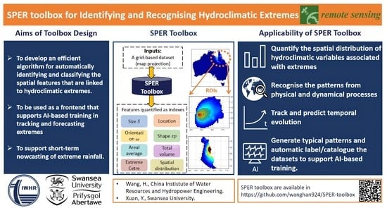
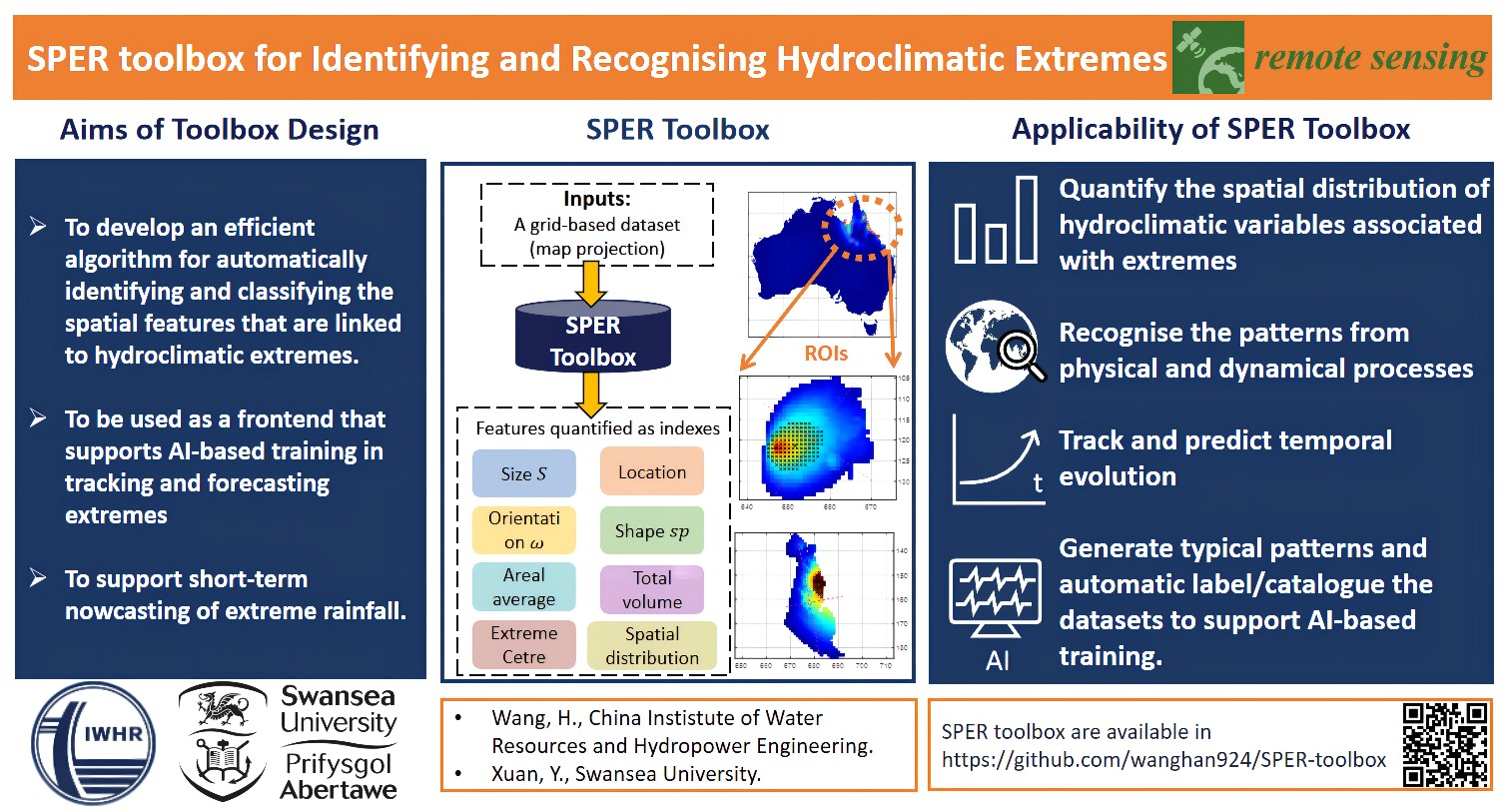
2.1. The Design of the SPER Toolbox

The Graphical User Interface (GUI) of the SPER toolbox and its main functions are presented in Figure 1. Users can load a grid-based hydroclimatic dataset such as precipitation, temperature, air humidity, wind speed, pressure values with a pair of linear spatial coordinates defined by a map projection, i.e., in a 2D matrix format, where the grid index is marked as ( x , y ) that indicates the location with respect to the origin at the upper left corner in a linear coordinate. Usually, a grid-based hydroclimatic dataset is defined on a map projection that has two mutually perpendicular directions, where the column of the matrix indicates the north-south direction y and the row indicates the east-west direction x . Additionally, the resolution as well as a threshold value (i.e., x 0 defined in Equation (1)) for extraction needs to be prescribed. Resolution, defined as the length of the grid in the x and y directions, is usually uniform applied in this toolbox. Figure 1a includes a case of extracting the spatial pattern of daily rainfall in Australia, where the inputs are grid-based daily rainfall with a resolution of 5 km and assumed to focus on the grid rainfall higher than or equal to a threshold x 0 = 35 mm. The next step is to extract the hydroclimatic variables (e.g., the daily rainfall) above the threshold located within a closed boundary which forms a region of interest (ROI). Then, the toolbox can automatically detect the location of each of such ROIs and quantify their spatial features, including the geographic location, size, orientation, and shape of the ROI, and the hydroclimatic features such as the areal average value, total volume, and spatial distribution of the hydroclimatic variable. SPER can also visualise the ROIs selected by the users among all detected ROIs (i.e., the right panel of GUI shown in Figure 1a). All the information of the ROIs extracted from the input datasets can be shown in the list of GUI and saved in a text file if needed. Figure 1b demonstrates the structure of the toolbox and specifies the inputs and example output. The details are presented in the following sections.

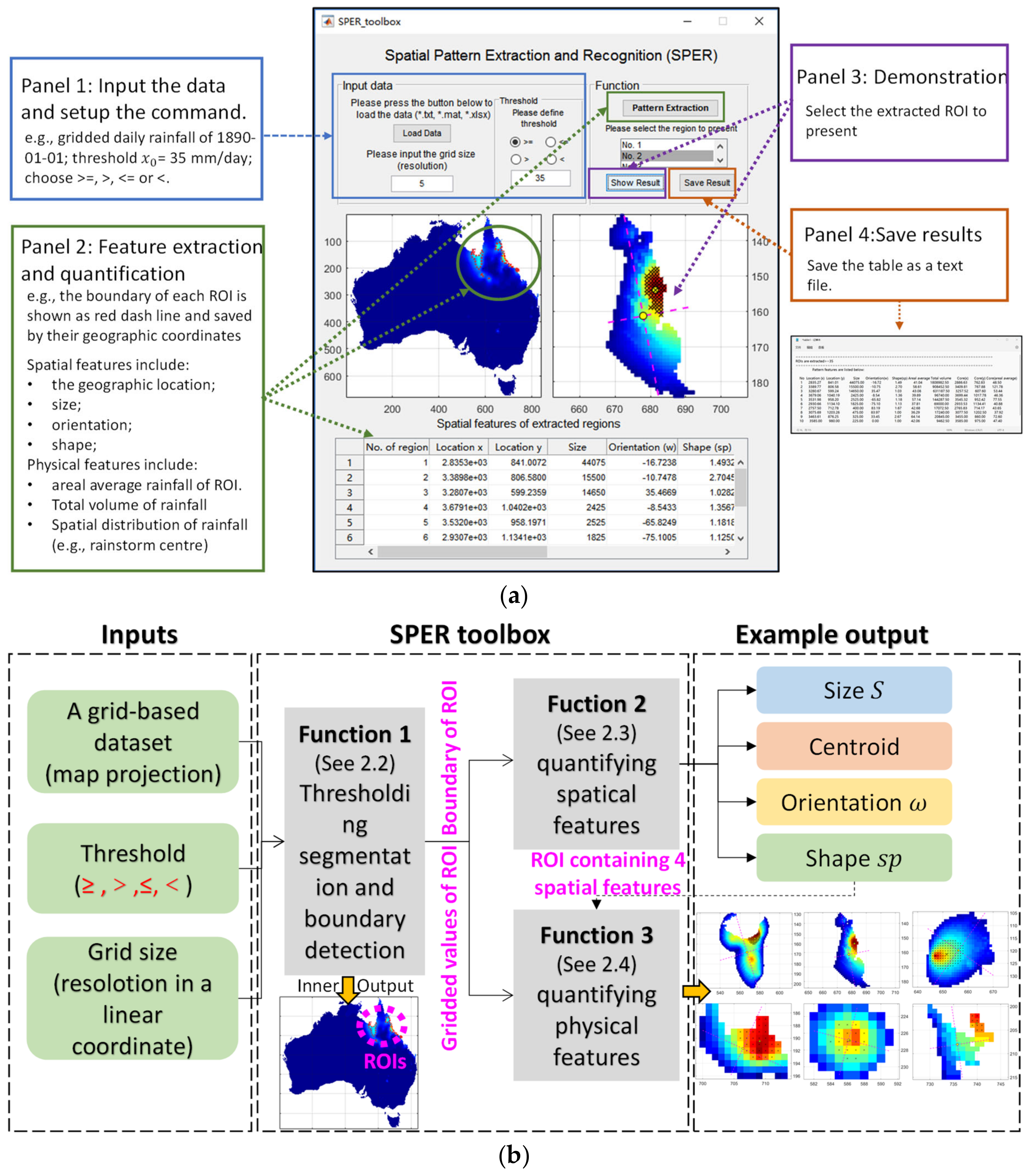
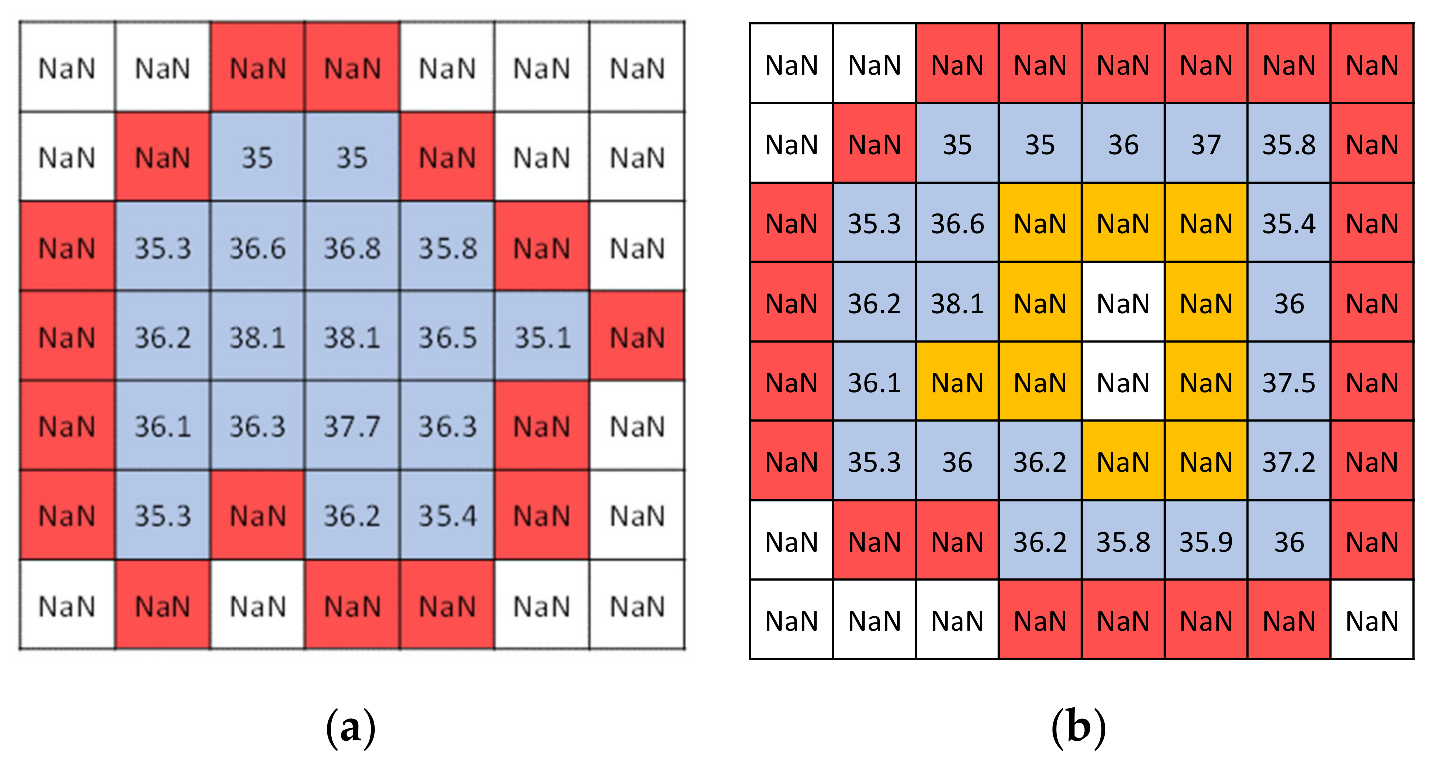
2.2. Thresholding Segmentation and Boundary Detection

Once the threshold value x 0 is defined, the first step of segmentation is to subdivide the grid-based dataset into constituent regions, the so-called regions of interest (ROIs). A widely used method of extracting an object from the background is to distinguish its different modes according to the threshold x 0 . Following this, the toolbox converts the dataset into a set of grids where any grid x , y for which f x , y is identified as an object grid otherwise a background grid. Thus, the new dataset g can be defined as four cases depending on different study purposes:
g x , y = f x , y ,   if   f x , y x 0 NaN ,           if   f x , y < x 0
g x , y = f x , y ,   if   f x , y > x 0 NaN ,           if   f x , y x 0
g x , y = f x , y ,   if   f x , y x 0 NaN ,           if   f x , y > x 0  
g x , y = f x , y ,   if   f x , y < x 0 NaN ,           if   f x , y x 0
where NaN means no data, which indicates the background. Equation (1a) presents the case focusing on the ROIs whose grid values are greater than or equal to the threshold, e.g., for identifying high intensive rainfall with a certain value; (1b) presents the case over the threshold, e.g., for identifying the rainfall regions; (1c) presents less than or equal to the threshold, e.g., for identifying cold cloud regions from satellite IR brightness temperature; 1d presents less than the threshold, e.g., for identifying less-than- 0   o C cold regions.
Then, the segmentation is carried out based on the discontinuity and similarity of the grid values of the dataset. Discontinuity is defined as an abrupt change in grid values nearby, which can be used for detecting the overall boundary, i.e., the boundary to distinguishing the ROI composed of the grids whose value is greater than or equal to x 0 and the background with the grids equal to NaN. In this case, to reduce the computation workload, NaN has been automatically assigned to the grids outside the ROIs then the abrupt change can be easily found and the overall boundary can be defined. A sketch example is presented in Figure 2a where for the new dataset g , an isolated ROI where f x , y 35 (blue grids) is defined as an area with similar property and its boundary is detected by an abrupt discontinuity (highlighted as red grids in the sketch a), where no data are found.
If some background grids ( f x , y < 35 ) are found to reside within the ROI boundary, the area that consists of these grids will form a “hole”. Holes can also be detected straightaway based on the discontinuity in grid values. An example of such is shown in Figure 2b, where the yellow grids are the hole boundary, while the blue grids are the ROI, which is an interconnected region with grid values greater than the predefined threshold. The information of each boundary (e.g., the coordinates of the boundary grid) is recorded separately and stored.

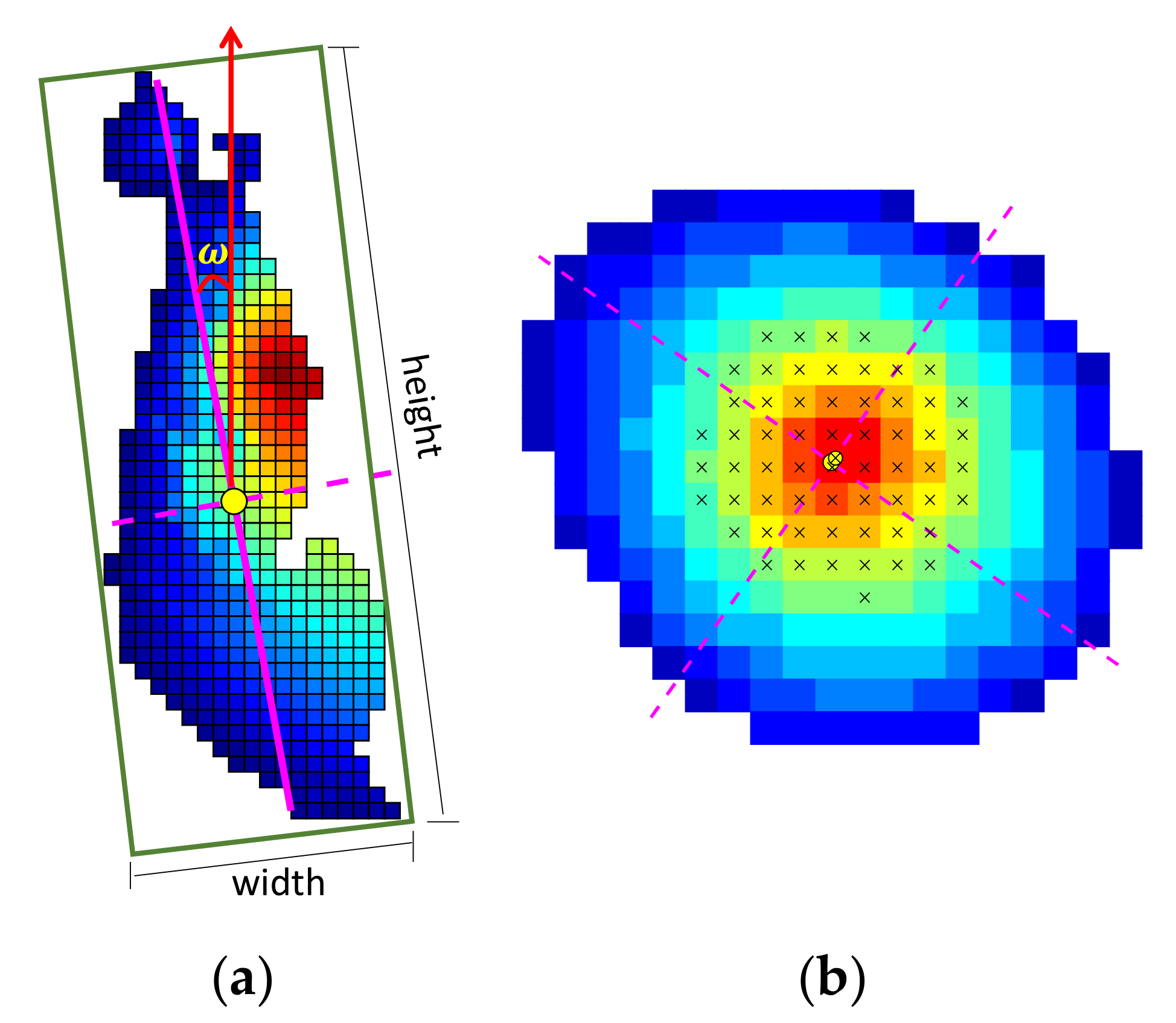
2.3. The Algorithm for Extracting and Quantifying the Spatial Features of the ROI

Each ROI extracted automatically from the previous step can be simplified as an irregular polygon. We developed an algorithm to quantify their spatial features (i.e., geophysical location, size, orientation and shape), which consist of the following four steps:
Step 1: Decompose the irregular ROI inside the boundary ( x j , y j ) into many (e.g., i ) small regular polygons A i , such as rectangles or triangles, and then the geometric centroid ( C x , C y ) of the ROI can be calculated as:
C x = C i x A i / A i = I x / A i = 1 6 j = 1 n x j y j + 1 x j + 1 y j y j + y j + 1 / A i  
C y = C i y A i / A i = I y / A i = 1 6 j = 1 n x j y j + 1 x j + 1 y j x j + x j + 1 / A i  
where n is the number of vertices of the irregular ROI, i.e., the number of boundary points in ( x j , y j ); C i indicates the centroid of each divided polygon and C x and C y mean the distance of the centroid from the y-axis (the vertical axis) or the x-axis (the horizontal axis); C i x A i and C i y A i are also known as the first moment of the area with respect to y and x ; A i is the total area of an ROI, which is the sum of the area of divided polygons; I x and I y are the inertia of the ROI to the x and y axes.
Step 2: Calculate the second moment of the area of the ROI. This moment is used to define the two principal axes of the ROI and the rotation, thereby obtaining the orientation of the ROI. The second moment of an area with respect to its centroid ( C x , C y ) is given by [15]:
I x x = 1 12 j = 1 n x j y j + 1 x j + 1 y j y j 2 + y j y j + 1 + y j + 1 2 I y 2 / A i
I y y = 1 12 j = 1 n x j y j + 1 x j + 1 y j x j 2 + x j x j + 1 + x j + 1 2 I x 2 / A i
I x y = 1 24 j = 1 n x j y j + 1 x j + 1 y j x j x j + 1 + 2 x j x j + 2 x j + 1 x j + 1 + x j + 1 x j I x I y / A i
As the two principal axes of an arbitrary polygon are those along which the product of inertia is zero, the orientation of the principal axes with respect to the centroid and the horizontal x-axis can be calculated as:
θ = 1 2 t a n 1 2 I x y / I y y I x x
where θ is measured positive anticlockwise from the centroidal x-axis. The other principal axis is just perpendicular to this.
Step 3: Determine the direction of the longer principal axis as the main orientation of the ROI. This direction is represented by the angle between the main orientation and the north direction, denoted as ω . ω is defined in the range of [−90°, +90°], where a positive value indicates a north-east direction, and a negative presents a north-west direction. Figure 3a provides an example where the orientation of this ROI is indicated by the solid principal axis, which is the longer one and orientated north-northwest ( ω = 10.4 o ).
Step 4: Determine the minimum encompassing rectangle of the ROI (see Figure 3a), which is used to characterise the elongation of the ROI. In this step, a shape index s p is introduced to represent how elongated (or narrow) the shape is. It is defined as the ratio of the longer side (e.g., height) of the encompassing rectangle divided by the shorter side (e.g., width). The greater the s p is, the more elongated an ROI is.
Finally, the spatial features extracted from this four-step algorithm are quantified as: (1) the geographic location of the ROI, which is represented by the coordinates of the geometric centroid C x , C y ; (2) the ROI size, which is the total number of grids times the grid size; (3) the ROI orientation, which is indicated by the angle ω with respect to the north direction and (4) the ROI shape, which is described by s p . All features are converted automatically consistent with the dataset resolution.

2.4. The Algorithm for Quantifying the Physical Features of the ROI

For a given ROI, its basic features such as the areal average value and integral over time of the hydroclimatic variable can be extracted directly by calculating the values of the grids. To quantify the spatial distribution of the hydroclimatic variable in the ROI, the k-means clustering technique is employed to recognise the centroid of the region(s) with the area called “core” that involves the relative high grid values. For example, if the dataset is grid-based hourly rainfall, the “core” with relatively high values inside an ROI can be regarded as the rainfall centre of this event whose location and the moving track can be easily monitored by the toolbox.
The k-means clustering is one of the partitioning-based techniques used to divide the variables of a dataset into non-overlapping clusters according to the degree of similarity of the variables [16,17]. The vectors of the ROI with several features, i.e., the centroid, boundary and grid-based hydroclimatic values are inputted and the clustering process starts by determining the number of clusters, which is usually based on the prior knowledge of the dataset. Since such information is often unavailable, in this toolbox, we designed multiple trials to find the optimal number of clusters k evaluated by using the Calinski–Harabasz criterion [18]. Then, the k-means++ algorithm is carried out to partition the data by assigning an initial centroid uniformly at random locations from the dataset, and the distance of each grid to this centroid is calculated. A new set of centroids are then selected again randomly but this time with a probability proportional to the distance from themselves to the closest centroid that is obtained from the previous step. This step is repeated until k centroids are selected. Compared with the k-means algorithm, this algorithm achieves a faster convergence and reduces the uncertainty caused by randomly selecting the initial centroids. Although the k-means++ algorithm has improved the quality of the final result to some degree, it in general still is local search heuristics meaning it can be sensitive to the initial centroids [19]; therefore, we repeat the procedure 10 times with different initial centroids to get relatively stable results and finally the result with the lowest distance is used.
The distance between the core(s) and the ROI centroid is then calculated and indicated as the spatial deviation of the rainfall event centre from the rainfall area centre, as shown in Figure 3b where the areal average of rainfall is 29 mm/day, and the rainfall centre (i.e., the core) is 38 mm/day marked by × which sits very closed to the centroid of the ROI.

3. Results

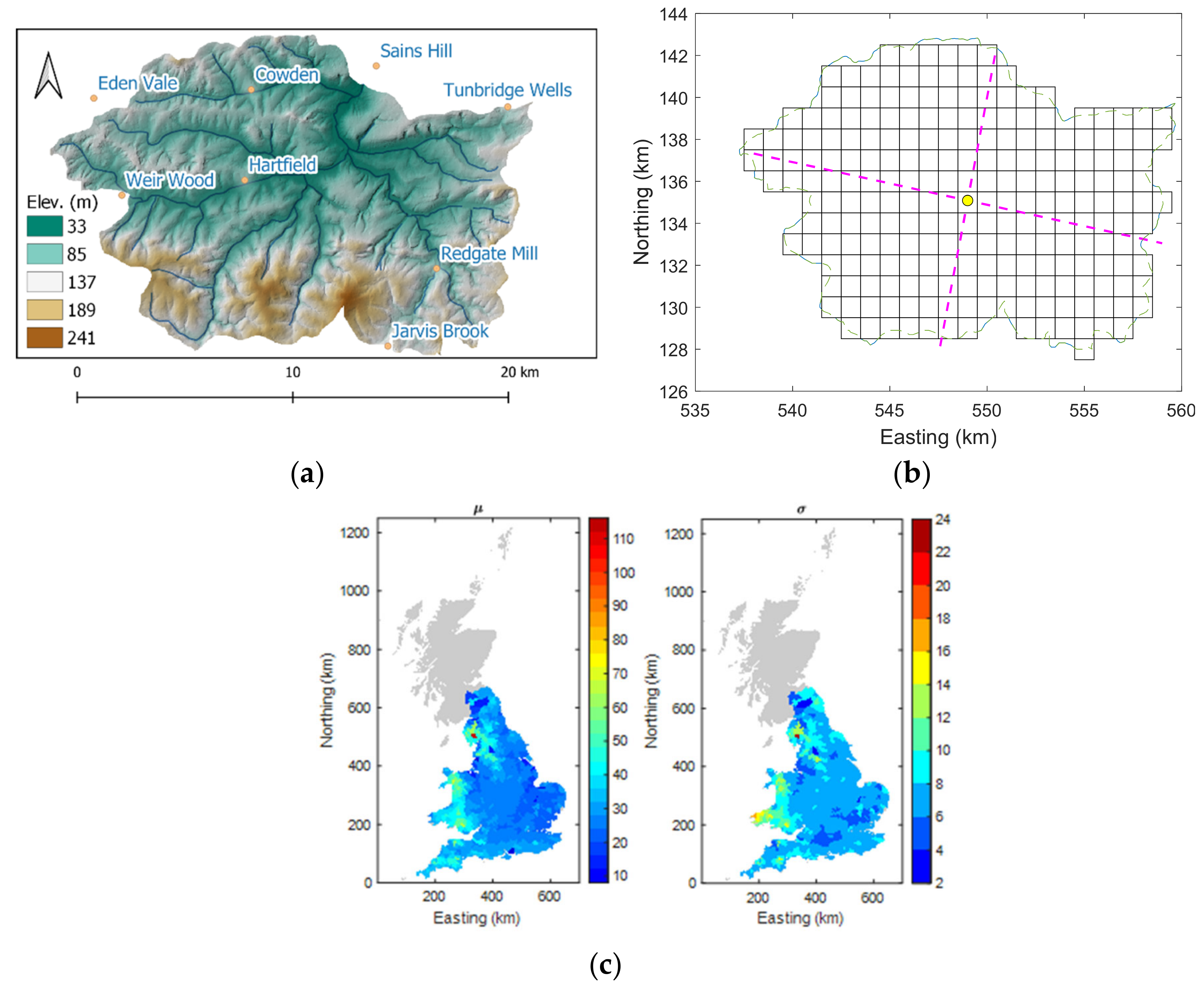
3.1. Illustrative Case 1: Catchment-Orientated Extreme Rainfall Variation in England and Wales

Atmospheric water content, precipitation, evaporation and transpiration, and surface water are four fundamental components of the hydrological cycle. To investigate the hydrological process, it is customary to focus on a region of interest, e.g., country, political city, river basin and even globally. Catchment is among the basic units in quantitative hydrological analysis. In any given catchments, runoff starts to be produced when the soil is saturated and cannot absorb the input water such as precipitation. Therefore, the area-oriented variation of rainfall is of concern of engineers and flood risk managers. Many studies, therefore, have focused on the catchment-based analysis that involves the estimation of the volume, area, and depth of rainfall within the catchment. For example, Ochoa-Rodriguez [20] investigated the impact of rainfall input resolution on the outputs of different hydrodynamic models of seven urban catchments in northwest Europe and found that increasing the catchment drainage area will decrease the impact of rainfall input resolution. Further, many other researchers analysed gauged rainfall extremes corresponding to their hydrological response in river catchments of different sizes [21,22,23].
The SPER toolbox can be useful in supporting analysing spatial variation within a specific boundary by providing a function for detecting spatial characteristics of a catchment or region of interest. Thus, in this first case study, we made use of the toolbox to conduct an analysis of the spatial variation of extreme rainfall in 903 catchments in England and Wales where the catchment’s boundaries were already given. The main aim of this study is to explore whether and how the quantification of extreme rainfall will be affected by the spatial features of the predefined regions such as the catchment. Firstly we extracted the spatial features of these 903 catchments and then quantified the long-term annual maximum daily rainfall (AMDR) in each catchment over the last century by using a well-tested generalised extreme value (GEV) distribution where the features of AMDR are parameterised by two distribution parameters μ and σ . These two parameters indicate the AMDR with the most frequent occurrence and somehow occurrence probability of the extremes, respectively. Finally, we studied how these two parameters vary with the spatial features and more details can be referred to [24]. Figure 4a,b present one of these catchments: the Upper Medway Catchment located in the southeast of England. The spatial features of this catchment detected by the toolbox are: (1) centroid location is indicated as (Easting 549 km, Northing 135 km) referring to the geographical origin [24] starting from the location of 400 km west, 100 km north of the true origin (49°N, 2°W); (2) the size is 230 km2; (3) the orientation is northeast-by-north (12.5° from the north); (4) the shape is elliptical ( s p = 1.56). Then, we extracted the gridded daily rainfall of this catchment from a century-long grid-based dataset [25] and did the same analysis for all the catchments and investigated how these spatial features affect the quantification of AMDR, which is presented in Figure 4c.
The results show that:
In England and Wales, most catchments (approximately 99%) are less than 600 km2 in size and more than half the catchments (61%) are relatively rounded or elliptical in shape. Those catchments near coastal regions tend to be northeast or northwest while inland—the boundary of England and Scotland is north-south orientated.
The change in the most frequent level of AMDR and the occurrence probability of the extremes over catchment sizes is not only affected by the size, i.e., increasing catchment size can decrease the level of most frequent AMDR because of statistical areal average, but also their geographic locations, e.g., when increasing size by involving more grids of higher rainfall can overcompensate the reduction caused by areal averaging. Compared with the geographic locations and sizes of the catchment, the effect of catchment orientation and shape is not as significant.

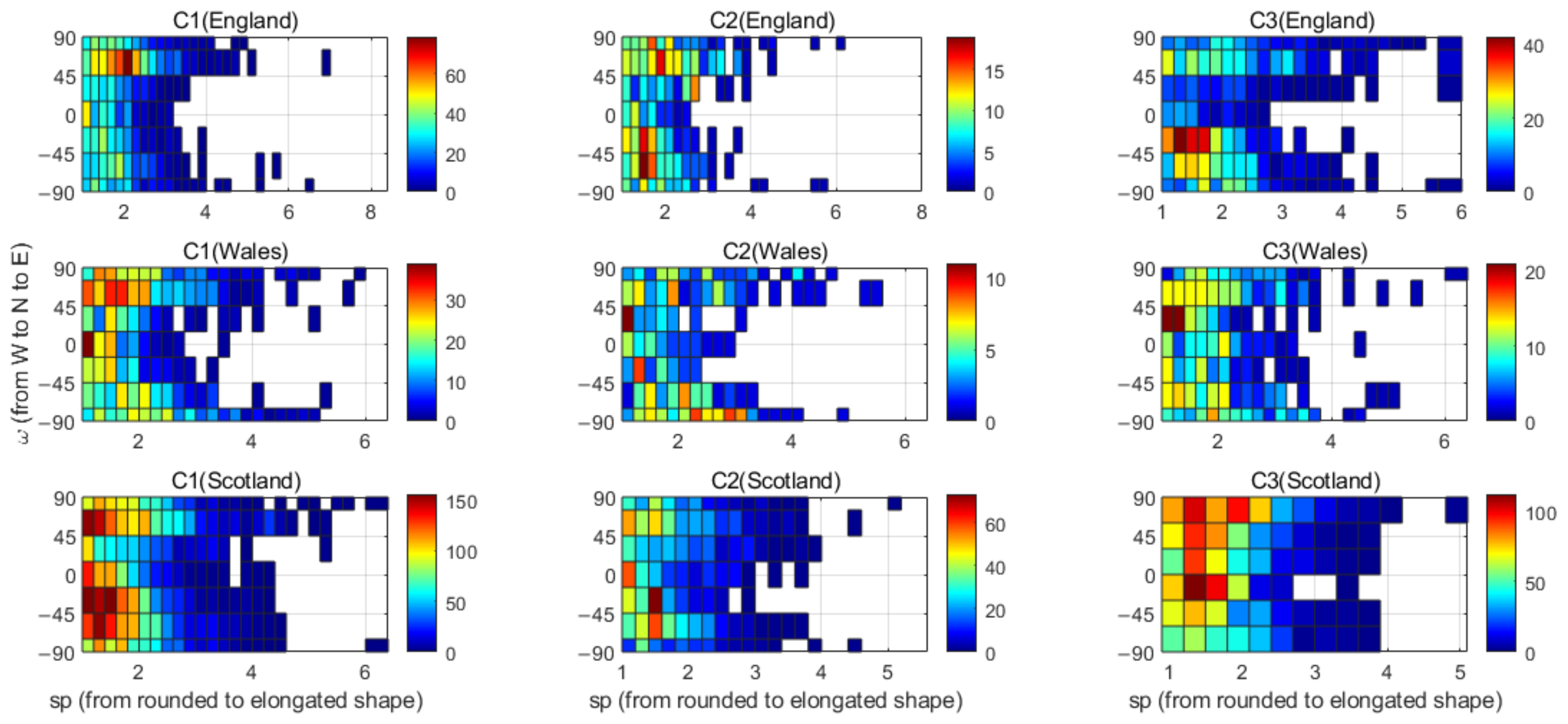
3.2. Illustrative Case 2: Pattern Recognition of Daily Rainfall over the Last Century in Great Britain

Although the spatial and temporal distributions of rainfall are affected by many hydrometeorological processes and different topographic conditions [26], they are usually bounded within specific patterns due to the relatively stable large-scale structure of atmospheric circulation. In this respect, the SPER toolbox becomes useful in helping explore the spatial variation of these patterns of rainfall distribution. In this case study, we made use of the GEAR dataset [25] from 1898 to 2010 over Great Britain (GB), and employed the SPER toolbox to extract the spatial features of daily rainfall in England, Wales and Scotland, respectively. Finally, all patterns were classified and the dominating patterns over the last century of GB were identified.
The rainfall area within a closed boundary is defined and recognised as an independent pattern where the SPER toolbox further extracted the rainfall area’s location, size, orientation and shape, and centre. These features are used to define the similarity among the patterns upon which feature-based grouping can be carried out. The location of the pattern (i.e., the geometric centre) was used to present where the rainfall is, e.g., in England, Wales and Scotland. Then, all recognised patterns are grouped into three groups by the size of rainfall area, i.e., the rainfall area smaller than 250 km2, between 250 and 500 km2 and those greater than 500 km2. The number of rainfall patterns in the three countries with respect to their orientation and shape is counted (see the histogram in Figure 5 where the colour indicates the number of each category) and the dominating features are identified as those ROIs with the most frequent occurrence (i.e., the ones with the greatest number shown in Figure 5). The patterns with the dominating features are regarded as the dominating (leading) patterns of daily rainfall in England, Wales and Scotland. Some typical patterns with dominating features are chosen as the examples illustrated in Table 1.
In England, the most frequent rainfall patterns of smaller size are mainly oriented northeast to east with a more elongated shape (1.5 < s p   < 2.0). However, for patterns of larger sizes, the orientation of the elongation changes from mainly northwest-by-west ( ω   −75°) to northwest-by-north ( ω −45°). This finding may be explained by the dynamics of the rainfall systems in various sizes. Small-sized rainfall distribution is likely to be driven by more localised convective storms which tend to have a more regular shape. Large rainfall systems may come as a result of frontal systems hence having a narrow band shape. Another very interesting feature is that intensive rainfall usually happens over a small region. The other two typical patterns of middle size in England are usually located in the vicinity of the Lake District. Those larger than 500 km2 in size usually cover the whole south of England.
In Wales, the typical pattern in the group smaller than 250 km2 in size is more rounded with a slight north–south orientation, while the patterns in the middle-sized group become more northeast-by-east-orientated and less rounded usually with a concave in the north-west direction because of topographic effect. These patterns also have a relatively fixed location at the northwest of Cardiff near the boundary of Wales and England (location index is easting 350 km, northing 250 km). For the patterns with a size larger than 500 km2, they are shown to have a very common “L” shape, which is almost across the north and south of Wales. It should be noted that the underlying dataset is in fact ‘masked’ by the land boundary; therefore, patterns of large size are artificially limited by the shape of the land.
In Scotland, the patterns whose size is smaller than 125 km2 are also more rounded and usually located to the north of the Lake District and near the boundary of England and Scotland. The middle-sized patterns whose orientation is nearly identical to those of smaller rainfall patterns, having two common locations: one is to the north of Lake District, while the other is in the north of Highland. The patterns with a size of over 500 km2 are mainly northwest-orientated and normally cover the whole north and west of Highland.

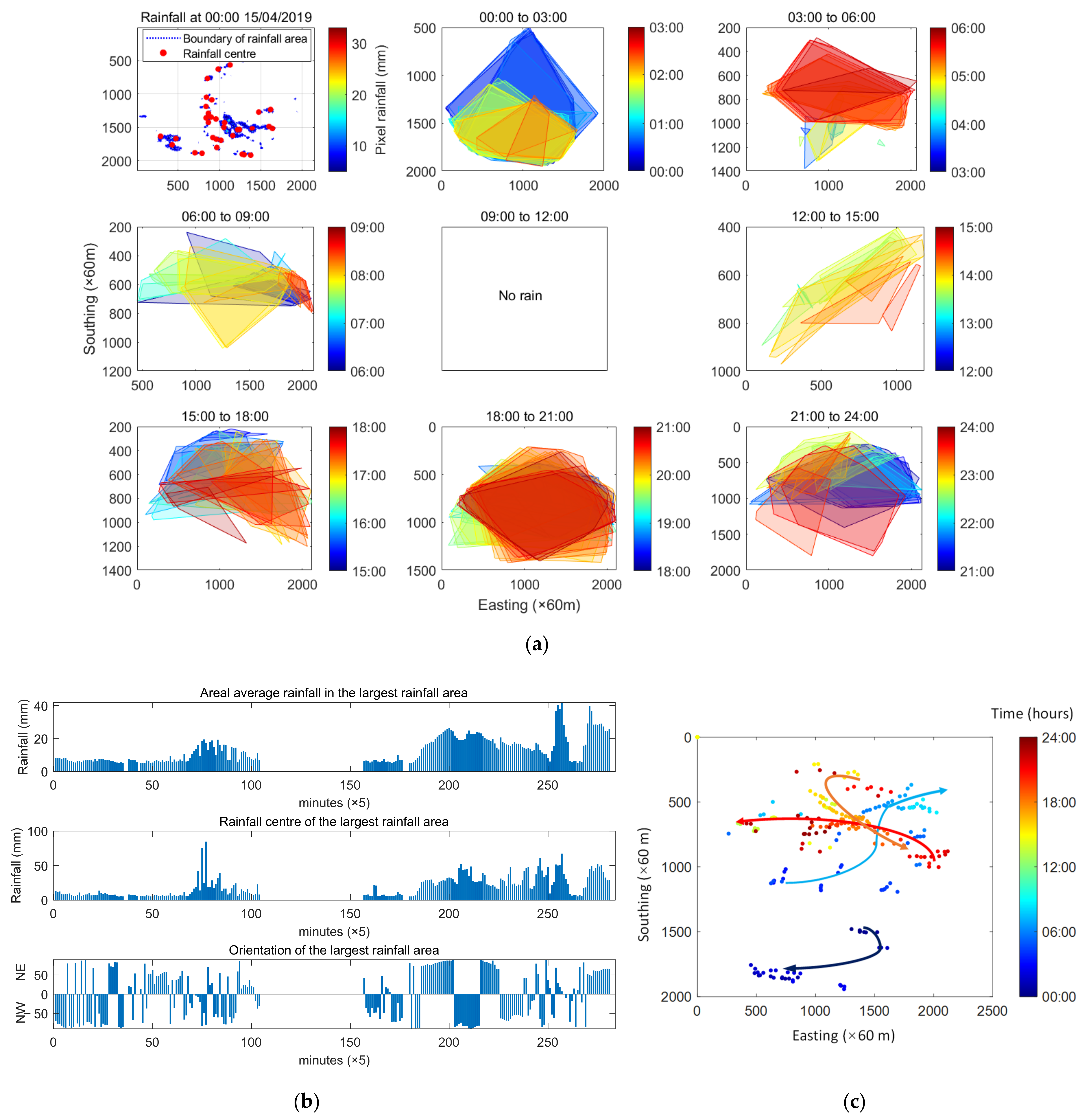
3.3. Illustrative Case 3: Tracing Rainfall Area and Spatial Distribution in 24 h in Guangdong, China

Rainfall is among the basic components of a hydrological circle where many studies focused on analysing its duration, intensity, and spatiotemporal variation to enhance the understanding of its interaction with the hydrological process. To monitor a rainfall event, traditional approaches often make use of rain gauge measurements to calculate the rainfall intensity and cumulative amount for characterising the rainfall behaviour [27,28,29]. However, the variability of rainfall is difficult to detect only by a limited number of rain gauges and the measurement affected by many factors such as wind and manual error can inevitably cause uncertainties even errors. In recent decades, with the rapid developments in environmental monitoring technology, weather radars with their high spatial and temporal resolution have been widely applied to monitor and measure rainfall [30,31]. The spatial and temporal patterns collected by weather radars are further used to model the rainfall event and the variability detected from the consecutive series of patterns can be used for forecasting. Therefore, identifying and tracking rainfall events are essential tasks for radar-based hydrometeorological applications and how to process it accurately and automatically is still a big challenge [32]. Nowadays, there are two types of algorithms for identifying and tracking rainfall patterns [33]: (1) the pixel-based algorithm, which makes use of pixel information and extracts the motion vectors by searching the maximum correlation coefficient of rainfall patterns in two consecutive radar images; (2) the object-based algorithm, which makes use of the properties of the discrete rainfall pattern such as centroid and area in consecutive radar images. However, both algorithms have drawbacks, e.g., the pixel-based algorithm can be easily affected by the noise; and the motion estimates solely based on the maximum correlation coefficient may produce inconsistent classification results, while the object-based algorithm is not good at estimating motions especially when the shape of rainfall pattern changes rapidly.
Therefore, a stable algorithm that can be used to classify and quantify the rainfall pattern is required. As the SPER toolbox can meet such needs, e.g., extracting hydrometeorological properties associated with rainfall patterns, this case study demonstrates how it can be used to monitor the rainfall area and trace the rainfall centres. Compared with most of other object-based algorithms, the SPER toolbox is able to extract not only the spatial features such as centroid, area, shape, but also the hydrometeorological properties such as the storm centre that would be more stable to track the motion and less affected by the rapidly changing shape. The data used in this case study are collected using the cutting-edge active phased array radar (APRA), which is among the latest developments in radar rainfall measurements with very high spatial-temporal resolution (e.g., 30 m and 30 s) and is suitable for small to medium, built-up areas. The advantage of APARs lies in that not only are they able to provide much-refined precipitation distributions, but they can be potentially used as a real-time driver for probabilistic flood forecasting and early warning systems. In this case, the radar rainfall observed on 15 April 2019 in Guangzhou, China is accumulated with resolutions of 5 min/60 metres and the SPER toolbox is used to detect the rainfall area.
The top left panel of Figure 6a presents the rainfall over a threshold ( 5 mm) at 00:00 local time, which is the start of radar measurement, and the red dots mark the rainfall centres (e.g., the core defined in Figure 3b). Then, we use an outer polygon to represent the area containing all these rainfall centres in the identified rainfall systems and the size and shape of the polygon can depict how this system is distributed over the study area. The rest sub-figures of Figure 6a show the changes in rainstorm centres in the rainfall system over space during the 24 h, where the colour of the areas indicates the elapsing time and a time step of 3 h is selected. The covering area (i.e., the outer polygon) can demonstrate how scattered all rainfall cells are, e.g., the larger coverage indicates the rainfall happened more scattered over space, while the smaller area indicates a more concentrated distribution of rainfall over space.
Since all rainfall cells are defined as a rainfall area over a predefined threshold within a closed boundary, they can be easily detected using similar steps of pattern recognition as discussed in Section 3.2. To monitor the movement of rainfall cells, we focus on those covering the largest area and present its characteristics such as the areal average rainfall, the rainfall at its centre, the orientation, and the moving track in Figure 6b, c. More comparison between the radar images (see Supplementary Materials Figures S2 and S3) and the SPER toolbox rainfall detection is described in Supplementary Materials Figure S1 and Text S1. It can be observed that the areal rainfall in the early nine hours of the day is generally lower than that of the last nine hours but the highest rainfall in the rainfall centre is in 06:00–07:00 when the areal rainfall is not very high. As for the area orientation, the majority show an east–west orientation or northwest-by-west or northeast-by-east, i.e., ω is near ± 90°, and the north–south orientation is rare in the 24 h. In addition, Figure 6c shows the tracking of the largest rainfall cell with colour-coded time stamps. These trajectories are derived by considering the centre locations of the largest rainfall cells within a short period, e.g., 30 min, and used for demonstrating the route and direction of the cells in 24 h. There are several rainfall systems detected: the rainfall cell with the largest area in first system located mainly in the south and moved towards west; in second system, more rainfall accumulates in the north and moved eastward; then a gap appeared where the rainfall stopped during the period approximately 9–13 h; the third system moved towards southeast, and the fourth system located in the north and moved westward.

4. Discussion

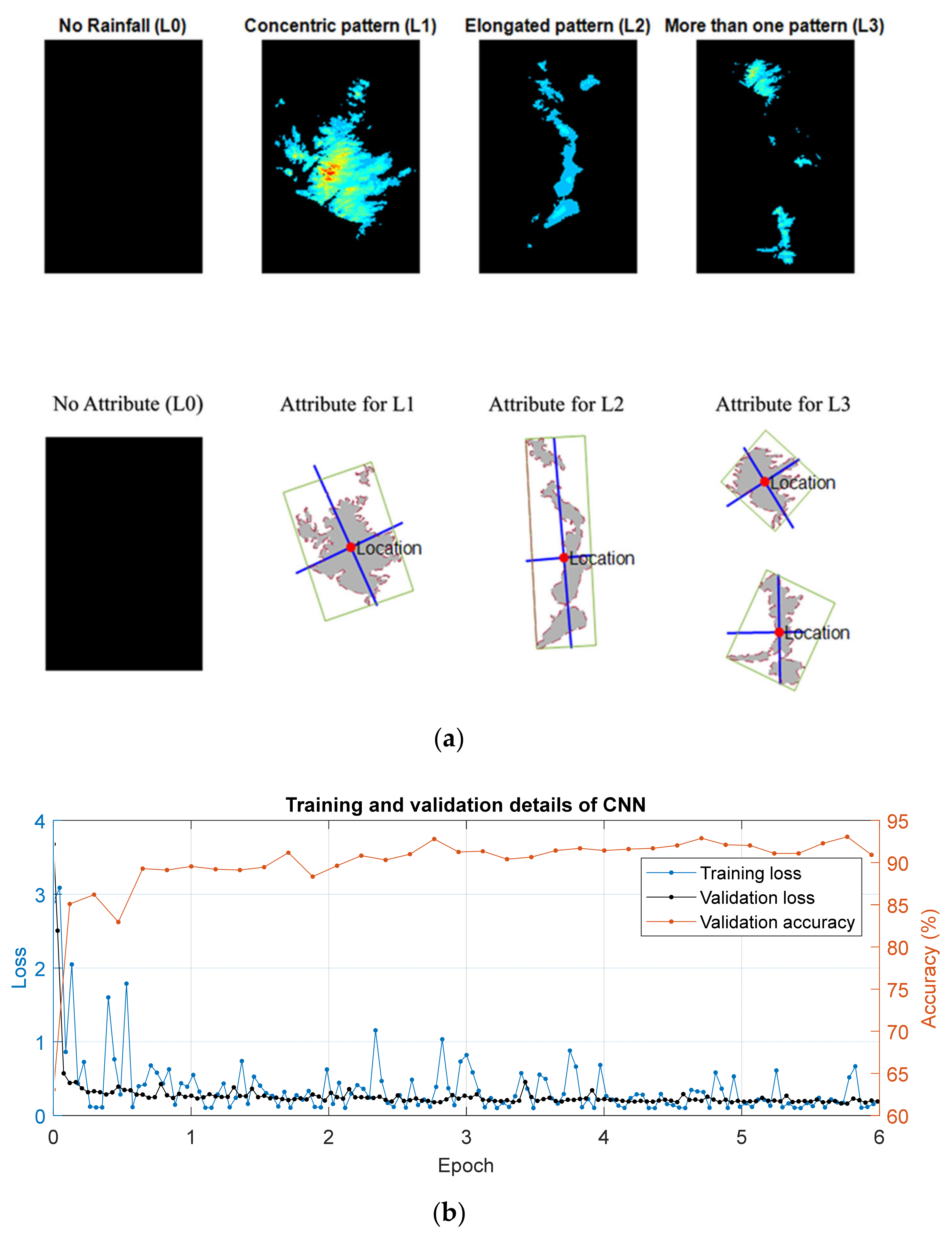
4.1. Potential Use as the Frontend of Supporting AI-Based Training

Identification and classification of hydroclimatic patterns are of great value to help understand the underlying mechanism and improve the forecasting capability, especially for those based on deep learning methods which have seen strong growth of applications recently.
For example, in hydroclimatic sciences, some researchers applied machine learning methods to extract spatiotemporal features and parameterise them to realise forecasts of climatic variables [34,35,36]. However, more efforts must be made in training the machine learning algorithms (e.g., ANN) before the well-trained technique can be applied to identify and classify the new data/images of hydroclimatic variables. This is also a huge challenge due to the data provided either by model simulations or via observations in hydrology are usually spatiotemporal, interconnected, non-linear, non-stationary, chaotic with high dimensions and large scales [14]. Therefore, it is in no doubt that manual diagnosing and processing of these data will require huge labour and time, if possible at all, and one must be aware of the complex properties of the hydroclimatic data/image before applying supervised method to identify the patterns. The SPER toolbox can address such needs automatically since its algorithms can detect the homo/heterogeneity of grid-based environmental data and extract spatial features identified as various indexes which can be readily used as the criteria for cataloguing. Users are allowed to pick up one or more indexes of interest to group a similar pattern. Such labelled groups can be further used for AI-based training.
To demonstrate and test the potential of the SPER toolbox being used to support AI-based training, we trained a convolution neural network (CNN) to detect the daily rainfall pattern in GB using four labels generated by the toolbox, i.e., no rainfall (L0), concentric pattern (L1) where its s p is near 1.0, elongated pattern (L2) and compound pattern (L3) which has both concentric and elongated types (see Figure 7a). Then, the trained CNN is tested by a set of 1166 new daily rainfall images of GB. The track of training and validation results are shown in Figure 7b where the training loss and the validation accuracy vary dramatically during the first epoch with 680 iterations then gradually converge to 0.17 and 92.5%. The toolbox has been shown to reach a test accuracy of 93.4% in classification, i.e., with 1089 out of 1166 new rainfall images having been classified correctly. More details on building and training CNN are provided in Supplementary Materials Text S2.

4.2. Limitations and Recommendations to Further Work

The SPER toolbox is designed mainly for extracting patterns from map projected data, i.e., with linear spatial coordinates, usually at local or regional scale with high resolution. The toolbox has been well tested by the three illustrative cases which show a good performance in dealing with these types of data and recognising the patterns effectively. Although the current version of the toolbox cannot fully address the inherent complexities of the hydrometeorological data that are sometimes chaotic, multilayer or lack enough detail and can cause complicated problems, it provides a useful tool to detect the homogeneous or heterogeneous pattern and quantify the similarity by parameterising its spatial and physical features. Additionally, being an unsupervised method, it requires less labour or time compared with training a supervised method such as CNN.
Therefore, further work is recommended to make the toolbox more robust and compatible with large-scale dataset at various, often low resolutions, such as longitude-latitude data at global scale. Downscaling, down-sampling method, and function to transfer data format may need to be integrated. Additionally, further work can allow for input data being non-uniform and within non-perpendicular coordinates—for example, the longitude and latitude of the grid spacing can be different and the direction is not limited in north–south and east–west, such as the Level 2 satellite swath of cross-track scan and along-track scan [37]. Further, the shape of the pattern can be described in more ways than using only a single shape index, e.g., the indexes of irregularity, spikiness and spiral can be involved to indicate how much variance there is in the angular and vertex and whether there is an inner-helical shape. Instead of using bounding box to define the elongation of the shape, the method called “best-fit ellipse” [38] can generate an outer ellipse regardless of the impact of the outliers, which can be used in further work.

5. Conclusions

In this paper, we present the development of a new open-source toolbox for spatial pattern extraction and recognition (SPER) for automatic extracting and classifying hydroclimatic patterns by both their spatial features and hydroclimatic features. The main aims of designing the toolbox are (1) to develop an efficient algorithm for automatically identifying and classifying the spatial features that are linked to hydroclimatic extremes; (2) to be used as a frontend that supports AI-based training in tracking and forecasting extremes; and (3) to support short-term nowcasting of extreme rainfall.
The applications of the SPER toolbox are tested with several applications in various areas and it can be concluded that the toolbox is able (1) to provide an effective and accurate quantification of the spatial distribution of hydroclimatic variables encompassed by natural or political boundaries; (2) to recognise the spatial patterns and features arising from physical and dynamical processes associated with hydroclimatic variables and further tracking and predicting their temporal evolution; (3) to generate typical (leading) patterns from large datasets and further automatic label/catalogue the datasets to support artificial intelligence and machine learning technique by incorporating a supervised and non-supervised classification of the events. Further study can be recommended to (1) improve the compatibility of the toolbox to more different formats of input; and (2) to further applied in the analysis of rainfall features with climate change (e.g., using satellite images).
The source code of the toolbox as well as the example case given above are available on GitHub (https://github.com/wanghan924/SPER-toolbox, accessed on 4 August 2022). The source code is provided subject to a GPL V3 license. Use/fork of the toolbox is subject to proper acknowledgement as stated on the Webpage of the toolbox.

Supplementary Materials

The following supporting information can be downloaded at: https://www.mdpi.com/article/10.3390/rs14153823/s1, Text S1: Processing radar rainfall. Text S2: Generating the training sets and testing the deep learning study. Figure S1: Demonstration of the step processing radar images of 24 h rainfall in Guangdong in the morning (a) and afternoon (b). Figure S2: Animated radar images (threshold 5 mm). Figure S3: Animated raw radar images (without setting threshold). References [39,40,41] are cited in the Supplementary Materials.

Author Contributions

Conceptualisation, H.W. and Y.X.; methodology, H.W.; software, H.W.; validation, H.W.; formal analysis, H.W. and Y.X.; writing—original draft preparation, H.W.; writing—review and editing, Y.X.; supervision, Y.X.; project administration, Y.X.; funding acquisition, Y.X. All authors have read and agreed to the published version of the manuscript.

Funding

This research was funded by the Academy of Medical Sciences, Grant Ref: GCRFNGR4_1165. The Guangdong Radar data were provided by the UK-China joint project “Early Warning Systems for Urban Flooding in Chinese Mega Cities using Advanced Phased Array Radar” supported by the Royal Academic of Engineering, Grant Ref: UUFRIP-10021.

Data Availability Statement

The datasets for testing the toolbox were provided by the Centre of Hydrology and Ecology (CEH) and available in https://doi.org/10.5285/33604ea0-c238-4488-813d-0ad9ab7c51ca (accessed on 4 August 2022), and the details of the catchments can be found in https://nrfa.ceh.ac.uk/content/catchment-boundary-and-areas (accessed on 4 August 2022).

Acknowledgments

H. Wang would like to thank the Chinese Scholarship Council, China and the College of Civil Engineering, Swansea University, for the Ph.D. scholarships provided. All grants are gratefully acknowledged.

Conflicts of Interest

The authors declare no conflict of interest.

References

  1. Bárdossy, A.; Filiz, F. Identification of flood producing atmospheric circulation patterns. J. Hydrol. 2005, 313, 48–57. [Google Scholar] [CrossRef]
  2. Montanari, A. Hydrology of the Po River: Looking for changing patterns in river discharge. Hydrol. Earth Syst. Sci. 2012, 16, 3739–3747. [Google Scholar] [CrossRef] [Green Version]
  3. Shaharudin, S.; Ahmad, N.; Zainuddin, N.; Mohamed, N. Identification of rainfall patterns on hydrological simulation using robust principal component analysis. Indones. J. Electr. Eng. Comput. Sci. 2018, 11, 1162–1167. [Google Scholar] [CrossRef]
  4. Rinaldi, A.; Djuraidah, A.; Wigena, A.H.; Mangku, I.W.; Gunawan, D. Identification of Extreme Rainfall Pattern Using Extremogram in West Java. IOP Conf. Ser. Earth Environ. Sci. 2018, 187, 012064. [Google Scholar] [CrossRef]
  5. Panu, U.S.; Unny, T.; Ragade, R. A feature prediction model in synthetic hydrology based on concepts of pattern recognition. Water Resour. Res. 1978, 14, 335–344. [Google Scholar] [CrossRef]
  6. Bishop, C.M. Pattern Recognition and Machine Learning; Springer: New York, NY, USA, 2006. [Google Scholar]
  7. Qiu, M.; Zhao, P.; Zhang, K.; Huang, J.; Shi, X.; Wang, X.; Chu, W. A short-term rainfall prediction model using multi-task convolutional neural networks. In Proceedings of the 2017 IEEE International Conference on Data Mining (ICDM), New Orleans, LA, USA, 18–21 November 2017. [Google Scholar] [CrossRef]
  8. O’Gorman, P.A.; Dwyer, J.G. Using machine learning to parameterize moist convection: Potential for modeling of climate, climate change, and extreme events. J. Adv. Model. Earth Syst. 2018, 10, 2548–2563. [Google Scholar] [CrossRef] [Green Version]
  9. Gentine, P.; Pritchard, M.; Rasp, S.; Reinaudi, G.; Yacalis, G. Could machine learning break the convection parameterization deadlock? Geophys. Res. Lett. 2018, 45, 5742–5751. [Google Scholar] [CrossRef]
  10. Petersik, P.J.; Dijkstra, H.A. Probabilistic Forecasting of El Niño Using Neural Network Models. Geophys. Res. Lett. 2020, 47, e2019GL086423. [Google Scholar] [CrossRef]
  11. Liu, Y.; Racah, E.; Correa, J.; Khosrowshahi, A.; Lavers, D.; Kunkel, K.; Wehner, M.; Collins, W. Application of deep convolutional neural networks for detecting extreme weather in climate datasets. arXiv 2016, arXiv:1605.01156. [Google Scholar]
  12. Nayak, M.A.; Ghosh, S. Prediction of extreme rainfall event using weather pattern recognition and support vector machine classifier. Theor. Appl. Climatol. 2013, 114, 583–603. [Google Scholar] [CrossRef]
  13. Nguyen-Le, D.; Yamada, T.J. Using weather pattern recognition to classify and predict summertime heavy rainfall occurrence over the Upper Nan river basin, northwestern Thailand. Weather Forecast. 2019, 34, 345–360. [Google Scholar] [CrossRef]
  14. Chattopadhyay, A.; Hassanzadeh, P.; Pasha, S. Predicting clustered weather patterns: A test case for applications of convolutional neural networks to spatio-temporal climate data. Sci. Rep. 2020, 10, 1–13. [Google Scholar] [CrossRef]
  15. Hally, D. Calculation of the Moments of Polygons. 1987. Available online: https://apps.dtic.mil/sti/citations/ADA183444 (accessed on 4 August 2022).
  16. Friedman, J.; Hastie, T.; Tibshirani, R. The Elements of Statistical Learning; Springer Series in Statistics; Springer: New York, NY, USA, 2001; Volume 1. [Google Scholar]
  17. Pham, D.T.; Dimov, S.S.; Nguyen, C.D. Selection of K in K-means clustering. Proc. Inst. Mech. Eng. Part C J. Mech. Eng. Sci. 2005, 219, 103–119. [Google Scholar] [CrossRef] [Green Version]
  18. Caliński, T.; Harabasz, J. A dendrite method for cluster analysis. Commun. Stat.-Theory Methods 1974, 3, 1–27. [Google Scholar] [CrossRef]
  19. Morissette, L.; Chartier, S. The k-means clustering technique: General considerations and implementation in Mathematica. Tutor. Quant. Methods Psychol. 2013, 9, 15–24. [Google Scholar] [CrossRef] [Green Version]
  20. Ochoa-Rodriguez, S.; Wang, L.P.; Gires, A.; Pina, R.D.; Reinoso-Rondinel, R.; Bruni, G.; Ichiba, A.; Gaitan, S.; Cristiano, E.; van Assel, J. Impact of spatial and temporal resolution of rainfall inputs on urban hydrodynamic modelling outputs: A multi-catchment investigation. J. Hydrol. 2015, 531, 389–407. [Google Scholar] [CrossRef]
  21. Anquetin, S.; Braud, I.; Vannier, O.; Viallet, P.; Boudevillain, B.; Creutin, J.-D.; Manus, C. Sensitivity of the hydrological response to the variability of rainfall fields and soils for the Gard 2002 flash-flood event. J. Hydrol. 2010, 394, 134–147. [Google Scholar] [CrossRef]
  22. Sangati, M.; Borga, M.; Rabuffetti, D.; Bechini, R. Influence of rainfall and soil properties spatial aggregation on extreme flash flood response modelling: An evaluation based on the Sesia river basin, North Western Italy. Adv. Water Resour. 2009, 32, 1090–1106. [Google Scholar] [CrossRef]
  23. Lobligeois, F.; Andréassian, V.; Perrin, C.; Tabary, P.; Loumagne, C. When does higher spatial resolution rainfall information improve streamflow simulation? An evaluation using 3620 flood events. Hydrol. Earth Syst. Sci. 2014, 18, 575–594. [Google Scholar] [CrossRef] [Green Version]
  24. Wang, H.; Xuan, Y. Spatial variation of catchment-oriented extreme rainfall in England and Wales. Atmos. Res. 2022, 266, 105968. [Google Scholar] [CrossRef]
  25. Tanguy, M.; Dixon, H.; Prosdocimi, I.; Morris, D.G.; Keller, V.D.J. Gridded Estimates of Daily and Monthly Areal Rainfall for the United Kingdom (1890–2015) [CEH-GEAR]. NERC Environmental Information Data Centre. 2016. Available online: https://catalogue.ceh.ac.uk/documents/33604ea0-c238-4488-813d-0ad9ab7c51ca (accessed on 4 August 2022). [CrossRef]
  26. Kirono, D.G.; Chiew, F.H.; Kent, D.M. Identification of best predictors for forecasting seasonal rainfall and runoff in Australia. Hydrol Process. 2010, 24, 1237–1247. [Google Scholar] [CrossRef]
  27. Muthusamy, M.; Schellart, A.; Tait, S.; Heuvelink, G. Geostatistical upscaling of rain gauge data to support uncertainty analysis of lumped urban hydrological models. Hydrol. Earth Syst. Sci. 2017, 21, 1077–1091. [Google Scholar] [CrossRef] [Green Version]
  28. Sohn, B.; Han, H.-J.; Seo, E.-K. Validation of satellite-based high-resolution rainfall products over the Korean Peninsula using data from a dense rain gauge network. J. Appl. Meteorol. Climatol. 2010, 49, 701–714. [Google Scholar] [CrossRef]
  29. Salio, P.; Hobouchian, M.P.; Skabar, Y.G.; Vila, D. Evaluation of high-resolution satellite precipitation estimates over southern South America using a dense rain gauge network. Atmos. Res. 2015, 163, 146–161. [Google Scholar] [CrossRef]
  30. Kidd, C.; Huffman, G. Global precipitation measurement. Meteorol. Appl. 2011, 18, 334–353. [Google Scholar] [CrossRef]
  31. Zhu, D.; Xuan, Y.; Cluckie, I. Hydrological appraisal of operational weather radar rainfall estimates in the context of different modelling structures. Hydrol. Earth Syst. Sci. 2014, 18, 257–272. [Google Scholar] [CrossRef] [Green Version]
  32. Sokol, Z.; Szturc, J.; Orellana-Alvear, J.; Popová, J.; Jurczyk, A.; Célleri, R. The role of weather radar in rainfall estimation and its application in meteorological and hydrological modelling—A Review. Remote Sens. 2021, 13, 351. [Google Scholar] [CrossRef]
  33. He, T.; Einfalt, T.; Zhang, J.; Hua, J.; Cai, Y. New Algorithm for Rain Cell Identification and Tracking in Rainfall Event Analysis. Atmosphere 2019, 10, 532. [Google Scholar] [CrossRef] [Green Version]
  34. Schultz, M.; Betancourt, C.; Gong, B.; Kleinert, F.; Langguth, M.; Leufen, L.; Mozaffari, A.; Stadtler, S. Can deep learning beat numerical weather prediction? Philos. Trans. R. Soc. A 2021, 379, 20200097. [Google Scholar] [CrossRef]
  35. Reichstein, M.; Camps-Valls, G.; Stevens, B.; Jung, M.; Denzler, J.; Carvalhais, N. Deep learning and process understanding for data-driven Earth system science. Nature 2019, 566, 195–204. [Google Scholar] [CrossRef]
  36. Cho, D.; Yoo, C.; Im, J.; Cha, D.H. Comparative assessment of various machine learning-based bias correction methods for numerical weather prediction model forecasts of extreme air temperatures in urban areas. Earth Space Sci. 2020, 7, e2019EA000740. [Google Scholar] [CrossRef] [Green Version]
  37. Salomonson, V.V.; Barnes, W.L.; Maymon, P.W.; Montgomery, H.E.; Ostrow, H. MODIS: Advanced facility instrument for studies of the Earth as a system. IEEE Trans. Geosci. Remote Sens. 1989, 27, 145–153. [Google Scholar] [CrossRef]
  38. Bergemann, M.; Jakob, C.; Lane, T.P. Global Detection and Analysis of Coastline-Associated Rainfall Using an Objective Pattern Recognition Technique. J. Clim. 2015, 28, 7225–7236. [Google Scholar] [CrossRef] [Green Version]
  39. Alom, M.Z.; Taha, T.M.; Yakopcic, C.; Westberg, S.; Sidike, P.; Nasrin, M.S.; Van Esesn, B.C.; Awwal, A.A.S.; Asari, V.K. The history began from alexnet: A comprehensive survey on deep learning approaches. arXiv 2018, arXiv:180301164. [Google Scholar]
  40. Krizhevsky, A.; Sutskever, I.; Hinton, G.E. Imagenet classification with deep convolutional neural networks. Adv. Neural Inf. Process Syst. 2012, 25, 1097–1105. [Google Scholar] [CrossRef]
  41. Pedamonti, D. Comparison of non-linear activation functions for deep neural networks on MNIST classification task. arXiv 2018, arXiv:180402763. [Google Scholar]
Figure 1. (a) The interface of the Spatial Pattern Extraction and Recognition (SPER) toolbox; (b) the structure, inputs, example output of the SPER.
Remotesensing 14 03823 g001
Figure 2. Two example sketches of an ROI, where f x , y 35 without (a) and with (b) a hole where the blue grids indicate the ROI and the red and yellow grids are the detected outer boundary and inner boundary (if there is a hole).
Remotesensing 14 03823 g002
Figure 3. (a) An example demonstrating the function of the SPER toolbox for defining the spatial features of the ROI: the location presented by the yellow circle, the orientation (major axis) presented by the solid magenta line, while the minor axis is presented by the dashed line, the shape defined by its encompassing rectangle. (b) An example demonstrating the core (marked by × ) of the ROI detected by the algorithm of quantifying the hydroclimatic features of the SPER toolbox. The colour indicates the value of rainfall from relatively high (red) to low (blue) above the threshold.
Remotesensing 14 03823 g003
Figure 4. Topographic and the river network map of the Upper Medway Catchment (a) and its spatial features (geographic location, size, orientation and shape) detected by the SPER toolbox (b) and spatial variation of parameters μ and σ of the GEV distribution for all catchments (c).
Remotesensing 14 03823 g004
Figure 5. The histograms of the number of daily rainfall patterns in England, Wales and Scotland are displayed in different colours with respect to s p and ω in three sizes (C1, C2 and C3).
Remotesensing 14 03823 g005
Figure 6. Monitor the rainfall changes in Guangdong in 24 h: the changes in the scattered area of rainfall centres (a), characteristics of the largest rainfall area (b) and the moving track of four rainfall systems (c).
Remotesensing 14 03823 g006
Figure 7. Four labels corresponding to the daily rainfall patterns: no rainfall (L0), concentric pattern (L1) where its s p is near 1.0, elongated pattern (L2) and compound pattern (L3) which has both concentric and elongated types (a); and the training and validation loss (blue and black lines) and validation accuracy (orange lines) of CNN (b).
Remotesensing 14 03823 g007
Table 1. Specific dominating patterns of daily rainfall in England, Wales, and Scotland catalogued in three sizes.
Location C 1
Size     250   km 2
C 2
250   km 2 < Size     500   km 2
C 3
Size > 500   km 2
England Remotesensing 14 03823 i001
s p : 1.5~2.0
ω : 45°~75°
Remotesensing 14 03823 i002
s p : 1.0~1.6
ω : −75°~−45°
Remotesensing 14 03823 i003
s p : 1.2~2.0
ω : −45°~−15°
Wales Remotesensing 14 03823 i004
s p : 1.0~1.2
ω : −15°~15°
Remotesensing 14 03823 i005
s p : 1.0~1.2
ω : 15°~45°
Remotesensing 14 03823 i006
s p : 1.0~1.4
ω : 15°~45°
Scotland Remotesensing 14 03823 i007
s p : 1.0~1.5
ω : −75°~−15°
Remotesensing 14 03823 i008
s p : 1.0~1.5
ω : −75°~−15°
Remotesensing 14 03823 i009
s p : 1.2~1.6
ω : −30°~0°
Publisher’s Note: MDPI stays neutral with regard to jurisdictional claims in published maps and institutional affiliations.

