
Multi-Sensor Sea Surface Temperature Products from the Australian Bureau of Meteorology


Australian Bureau of Meteorology, 700 Collins Street, Docklands, VIC 3008, Australia
*
Author to whom correspondence should be addressed.
Remote Sens. 2022, 14(15), 3785; https://doi.org/10.3390/rs14153785
Submission received: 6 July 2022
/
Revised: 2 August 2022
/
Accepted: 3 August 2022
/
Published: 6 August 2022
(This article belongs to the Special Issue Advances in Retrieval, Operationalization, Monitoring and Application of Sea Surface Temperature II)
Abstract
:Sea surface temperature (SST) products that can resolve fine scale features, such as sub-mesoscale eddies, ocean fronts and coastal upwelling, are increasingly in demand. In response to user requirements for gap-free, highest spatial resolution, best quality and highest accuracy SST data, the Australian Bureau of Meteorology (BoM) produces operational, real-time Multi-sensor SST level 3 products by compositing SST from Advanced Very-High-Resolution Radiometer (AVHRR) sensors on Meteorological Operational satellite (MetOp)-B and National Oceanic and Atmospheric Administration (NOAA) 18, along with SST from Visible Infrared Imaging Radiometer Suite (VIIRS) sensors on the Suomi National Polar-orbiting Partnership (Suomi NPP) and NOAA 20 polar-orbiting satellites for the Australian Integrated Marine Observing System (IMOS) project. Here we discuss our method to combine data from different sensors and present validation of the satellite-derived SST against in situ SST data. The Multi-sensor Level 3 Super Collated (L3S) SSTs exhibit significantly greater spatial coverage and improved accuracy compared with the pre-existing IMOS AVHRR-only L3S SSTs. When compared to the Geo Polar Blended level 4 analysis SST data over the Great Barrier Reef, Multi-sensor L3S SST differs by less than 1 C while exhibiting a wider range of SSTs over the region. It shows more variability and restores small-scale features better than the Geo Polar Blended level 4 analysis SST data. The operational Multi-sensor L3S SST products are used as input for applications such as IMOS OceanCurrent and the BoM ReefTemp Next-Generation Coral Bleaching Nowcasting service and provide useful insight into the study of marine heatwaves and ocean upwelling in near-coastal regions.
Keywords:
sea surface temperature; multi-sensor SST; composite SST; VIIRS; AVHRR; corals; great barrier reef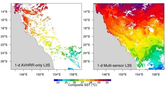
1. Introduction
Sea Surface temperature (SST) is an important geophysical factor that affects many physical and biological processes on the Earth. The heat from warmer water can significantly modify air masses close to the sea surface and influence the Earth’s atmosphere above. SST is widely used to understand, predict and monitor heat fluxes, momentum, salt and gas fluxes between the ocean and atmosphere [1,2]. It is a key factor in tropical cyclogenesis and plays an important role in the formation of sea fog and breezes [3]. Moreover, many biological and chemical processes are driven by temperature baselines, oceanic eddies and other currents and upwelling, which are strongly dependent on thermal gradients and near-surface warming [4,5]. Due to this and substantial socio-economic implications, there is increasing demand for gap-free, high-resolution sea-surface temperature observations from satellites for a wide range of applications, including research and environmental monitoring [6,7].
Several satellite sensors provide SST observations, including thermal infra-red radiometers on Sun-synchronous polar-orbiting and geostationary satellites and passive microwave radiometers on both non-Sun-synchronous orbiting and Sun-synchronous polar-orbiting satellites [8]. Microwave radiometers are subject to lower levels of atmospheric interference than infra-red radiometers. However, the size of the antenna that can be deployed on current satellites (typically 2 m or less in diameter), combined with limitations of the microwave frequencies that can be used to measure SST, results in a diffraction-limited surface resolution of SST observations that can be measured by these sensors. Current microwave sensors typically measure SST over pixels in the 20 to 60 km range with degradation of accuracy within 100 km of land [8]. This limits their application in near-coastal regions and near highly dynamic sub-mesoscale structures. In contrast, thermal infra-red sensors on low Earth orbit polar-orbiters produce operational SST products at a much higher spatial resolution, ranging from 0.25 to 1.1 km at nadir [8], allowing accurate observations to around 1 km from coasts. However, unlike passive microwave imagers, these infra-red sensors cannot sense SST under clouds and can be biased by aerosols [9]. A suite of environmental polar-orbiting satellites circles the Earth in Sun-synchronous orbits at altitudes of approximately 850 km. Each satellite visits each point on Earth twice daily, crossing the equator at the same local solar time each day (either am or pm). Several types of thermal infra-red sensors mounted on polar-orbiting satellites with different Equatorial Crossing Times (ECTs) provide SST data to spatial resolutions of 0.25 to 1.1 km at nadir. These sensors observe a limited area of the Earth during each orbit, and spatial coverage in composite SST products may be improved by merging data from satellite sensors that have different ECTs. Since clouds obscure the view of infra-red satellite sensors, compositing data from several satellite sensors acquired at different times between which clouds might have moved also results in better data coverage. These composite SST products are useful for many applications, including mapping coastal areas experiencing anomalous heating or cooling that may cause ecological impacts, fisheries management, ocean current mapping for ship navigation, ocean model validation and ecological research [6,7]. However, the continuous production of composite SST products over multiple years can be hampered as satellites have a limited life span, and early generation sensors are replaced by more advanced sensors. Our challenge is to add high-resolution data streams from new sensors to ongoing data products, for example, SST Climatology or SST composite and analysis products. The Advanced Very-High-Resolution Radiometer (AVHRR) is a passive infra-red sensor that has been carried continuously on NOAA’s series of Polar-Orbiting Environmental Satellites (POES) starting with the launch of NOAA-6 in 1981 and ending with the launch of NOAA-19 in 2009 [7]. In 2018, NOAA officially replaced the AVHRR sensor program with the Visible Infrared Imager Radiometer Suite (VIIRS) sensor program, with the first VIIRS instruments carried by the Suomi National Polar-orbiting Partnership (NPP) platform from October 2011 and NOAA-20 (N20) satellite from November 2017. In September 2018, the orbital decay of NOAA-19 resulted in transitioning the AVHRR sensor into a fully sunlit orbit [10], which has adversely affected its overall calibration and, therefore, accuracy [11].
At the Bureau of Meteorology (BoM), the High-Resolution Picture Transmissions (HRPT) AVHRR data received via ground stations in Australia and Antarctica from POES satellites NOAA-11 through to NOAA-19 are used to produce a range of IMOS Level 3 composite SST products on a 0.02× 0.02 grid over the Australian (70E to 190E, 70S to 20N) and Southern Ocean (2.5E to 202.5E, 77.5S to 27.5S) [7,12] domains. These have been used for a range of research and operational applications, including high-resolution climatology over the Australian region [13], marine ecological monitoring [7,14] and ocean temperature diurnal variation research [15]. Amongst these, the IMOS AVHRR Level 3 Super-Collated (L3S) SST products, formed using HRPT AVHRR data from multiple NOAA POES satellites, have been used as inputs into the IMOS OceanCurrent web application (http://oceancurrent.imos.org.au, accessed on 30 June 2022) and the BoM ReefTemp Next-Generation Coral Bleaching Risk service ([14], http://www.bom.gov.au/environment/activities/reeftemp/reeftemp.shtml, accessed on 30 June 2022). As the legacy AVHRR platforms degrade further and the desire for coverage remains strong, the BoM has started compositing SST data from new advanced satellite sensors with data from currently used sensors. These new “Multi-sensor Level 3 Super-Collated (L3S)” SST composites [12,16] cover the same Australian and Southern Ocean domains as the legacy AVHRR L3S composites became publicly available in real-time and delayed mode on 16th November 2018 and, from that time, replaced the AVHRR-only L3S SST composites as inputs into IMOS OceanCurrent and BoM ReefTemp Next-Generation Coral Bleaching Risk service. They have also contributed to research into Marine Heat Waves [17] and the oceanic drift of kelp [18] and have been incorporated into a valuable multi-decadal ocean temperature near-coastal time series [19]. The improvement in spatial coverage and accuracy afforded by the addition of sensors has enhanced the usefulness of the IMOS L3S SST composites and encouraged user uptake. This paper will report on Multi-sensor L3S from the Australian domain only as this is more commonly used.
The addition of data from more modern satellite sensors to the existing HRPT AVHRR SST data required a compositing method that would composite data from old and new satellite sensors together with appropriate quality assessment. The BoM currently produces operational Multi-sensor L3S SST products [12,20] in the Group for High-Resolution SST (GHRSST: http://ghrsst.org, accessed on 30 June 2022) Data Specification version 2.0 revision 5 (GDS2.0) format [16] using infrared data from the following Polar-orbiter infra-red sensor SST data streams (described in Section 2 and Section 3):
These data are sourced from different meteorological agencies, where systems process the raw data received by satellite ground stations differently to make their level 2 and level 3 SST products. They also use different quality assessment methods [16] for their SST products. To composite SSTs from different sources, the quality of all data needs to be reassessed so that all sensors can be treated uniformly. This paper describes the method that is being used at BoM for the composition of AVHRR and VIIRS SST data. Input data are described in Section 2. The method used to redefine the quality level of remotely-sensed SST data and the compositing method, where swaths from the same platform and sensors are composited together to form level 3 collated (L3C) products on the IMOS 0.02-degree grid, is described further in Section 2. During the day, SST can be modified by solar heating, whereas night-time observations are more stable and representative of the temperature near the surface skin interface. The daytime and night-time observations are composited separately and produce 1-day L3C composites for daytime and night-time for all available satellite platforms. Processing methods of how Multi-sensor level 3 Super-Collated (L3S) SSTs are constructed by compositing L3C SSTs from individual satellite sensors with redefined quality levesl for day-only, night-only and day and night scenarios are further described in Section 2. In Section 3, the results are discussed. The utility of the new Multi-sensor SSTs and their validation against in situ observations are described. As a case study, Multi-sensor L3S products are compared with NOAA’s Geo-polar blended level 4 (L4) statistically interpolated SST Analyses for the 2017–2018 period for the Great Barrier Reef region to check whether Multi-sensor L3S SSTs show better feature resolution than L4 SST products. Discussion and conclusions are described in Section 4 and Section 5, respectively.
2. Materials and Methods
2.1. Data
The following data are used to construct Multi-sensor L3S SST products.
2.1.1. AVHRR
Prior to the launch of MODIS on Terra (1999) and Aqua (2002), the only wide swath, 1-km resolution satellite SSTs available were direct-broadcast AVHRR SSTs. High spatial resolution satellite imagery for SST has been acquired around Australia and Antarctica since the mid-1980s, using direct broadcast HRPT from AVHRR sensors on the NOAA series of Polar-Orbiting Environmental Satellites. The native spatial resolution of SST measurements from the AVHRR series of sensors is 1.1 × 1.1 km at nadir, expanding to 2.3 × 6.2 km at the edge of the swath [7]. NOAA-18 was launched on 20 May 2005 and, with no fuel on board, is in a drifting orbit that currently crosses the equator several times per day at around 10:12 a.m. and 10:12 p.m. local time (as of 30 May 2022). In collaboration with the Commonwealth Scientific and Industrial Research Organisation (CSIRO), the Bureau processes HRPT AVHRR data from NOAA-18, received from Australian and Antarctic ground stations, and produces IMOS Level 2P (L2P), Level 3 Uncollated (L3U) and Level 3 Collated (L3C) SST products in real-time [12]. Although NOAA-18 is a relatively old satellite, and in spite of its orbital drift, given its relatively small errors since January 2019 (Section 6.2 of [11]) and good data coverage, it is currently ingested into operational and reprocessed Multi-sensor L3S SST products to enhance good quality data coverage.
NOAA-19 was launched on 6th February 2009. The satellite is still functional but has drifted into a fully sunlit orbit since September 2018 [10], which has adversely affected its accuracy. The data received by Australian and Antarctic ground stations are processed similarly to NOAA-18 for the satellite. The data from NOAA-19 were included in the reprocessed Multi-sensor L3S SST products until 3 September 2018.
NOAA-18 and NOAA-19 are the last in the series of operational POES satellites to carry AVHRR sensors, although they are still carried on the ESA MetOp series of polar-orbiters, MetOp-A, B and C. Due to data storage constraints on the POES satellites, the highest resolution POES AVHRR data are only available via direct download via line-of-sight from the satellites to ground stations, as either HRPT or Local Area Coverage (LAC) AVHRR transmissions. With the launch in October 2006 of an AVHRR sensor on the MetOp-A polar-orbiting meteorological satellite (ESA), it became possible, for the first time, to obtain global coverage Full-Resolution Area Coverage (FRAC) AVHRR SST data at a 1.1 km resolution at nadir.
The MetOp satellites were developed by the European Space Agency (ESA) and operated by the European Organisation for the Exploitation of Meteorological Satellites (EUMETSAT). The first MetOp satellite, Metop-A, was launched on 19 October 2006; Metop-B was launched on 17 September 2012 and Metop-C on 7 November 2018. Ifremer, as a EUMETSAT Ocean and Sea Ice Satellite Application Facility (OSI-SAF, http://www.osi-saf.org, accessed on 30 June 2022), provides FRAC AVHRR L2P SST products for MetOp-A, MetOp-B and MetOp-C. The BoM downloads and further processes these EUMETSAT-produced MetOp L2P SST data to produce IMOS MetOp AVHRR L3U and L3C and Multi-sensor L3S SST products. L2P SSTs from only one MetOp satellite at a time are available operationally from EUMETSAT OSI-SAF. Currently, MetOp-B is operational (available from [22] and is included in the Bureau’s current operational Multi-sensor L3S SST products. For reprocessing, MetOp-A data are used for the period 1 January 2012 to 19 January 2016, and Metop-B data are used after 19 January 2016. MetOp-C data are currently being tested for inclusion in the operational IMOS Multi-sensor L3S products.
2.1.2. VIIRS
In 2018, NOAA officially replaced the AVHRR sensor program with the VIIRS passive infra-red sensor. The VIIRS radiometer has a greater number of spectral bands than AVHRR and has a better spatial resolution, radiometric accuracy and stability than AVHRR [7]. The VIIRS is flown in an afternoon orbit (≈1:20 am/pm local time) to provide SST observations twice per day. The sensor has ≈750 m resolution at nadir and provides full global coverage with the use of a modern radiometer design with 16 channels, 5 of which have significant sensitivity to SST [8,25].
The first VIIRS sensor was launched in October 2011 onboard the NPP satellite. NOAA-20 (N20) is the second satellite carrying a VIIRS sensor. Launched in November 2017, N20 joined NPP in the same orbit. The time difference of approximately 50 min between the two satellites allows data coverage overlap [26]. The NOAA Satellite and Information Service (NESDIS) Office of Satellite and Product Operations (OSPO) operationally produces the Advanced Clear Sky Processor for Ocean (ACSPO) VIIRS 0.02 L3U SST product [27,28], developed by the NOAA/NESDIS Center for Satellite Applications and Research (STAR), with a grid aligned with the IMOS 0.02 L3U product for both NPP [23] and N20 [24]. At the Bureau, these files are downloaded and further processed to construct IMOS VIIRS L3U, L3C and the Multi-sensor L3S SST products (Section 2).
2.1.3. Ancillary Fields
- Wind Speed
The average 10 m wind speed estimated from numerical weather prediction models is used to define the high wind speed (>20 m/s) and low wind speed (<2 m/s) in ocean regions. Prior to 1 September 2009, the European Centre for Medium-Range Weather Forecasts (ECMWF) historical re-analysis [29] was used. While after 1 September 2009, the Australian Community Climate and Earth System Simulator-Global (ACCESS-G) 6-hourly analysis winds [30] are used.
- Sea Ice Fraction
The sea ice fraction used in the data files is taken from the NOAA National Centers for Environmental Prediction (NCEP) 1/12 sea ice analysis ([31])
- Foundation SST Analysis
The deviation between the SST and the level 4 analysis of the previous day’s foundation temperature is denoted as ‘dt_analysis’ in the SST data files. The Global Australian Multi-Sensor Sea Surface Temperature Analysis (GAMSSA, [32,33]) foundation SST is used as the level 4 analysis. GAMSSA is a daily analysis SST product available on a global 0.25 grid.
2.2. SST Processing Methods
The BoM produces two versions of all SST products—file version 1 (fv01) and file version 2 (fv02). Figure 1 gives an overview of the processing chain that was followed to construct both of these types of SST products.
fv01 is the near real-time operational SST product version that is published by IMOS for at least the last year of activity (currently, data are available from 1 January 2021). Data from all available operational satellite sensors are sourced from different meteorological agencies and are processed for this version of products. Currently, data from NOAA-18 (regressed against buoys, BoM), MetOp-B (radiative transfer model, EUMETSAT), NPP and N20 (regressed against buoys, NOAA) are processed for the fv01 product version SST products. Some fields and metadata may not be available in the fv01 SST products.
fv02 is the reprocessed SST product version, available in delayed mode, and is published by IMOS in the historical archives. This product represents a long time series product, substantially more complete than the fv01 product. It is produced with a variable (adaptive) regression-based retrieval with modelled Sensor-Specific Error Statistics (SSES: [16]) estimations for NOAA-11 from 19 platforms [12]. fv02 is processed in delayed mode to include any missing data that were not available at the time of processing the operational near real-time fv01. It is processed with a more comprehensive approach and has more fields compared to fv01 [12]. For processing fv02 L2Ps for NOAA-11 to 19 satellites, separate standard algorithms are used day and night, and a three-channel unified algorithm is used for the day and night scenario. It covers NOAA-11 to 20, MetOp-A, MetOp-B and NPP platforms, where NOAA-11 to 19 data are processed at the BoM, VIIRS data are sourced from NOAA and AVHRR MetOp data are sourced from EUMETSAT. The historical archive is updated when any additional data are available or when an updated processing method becomes available. Currently, fv02 data are available for the 1992–2020 period.
2.2.1. IMOS HRPT AVHRR L2P
IMOS AVHRR L2P products are formed from geolocated, cloud cleared and ungridded AVHRR single swath SST data (https://imos.org.au/facilities/srs/sstproducts/sstdata0, accessed on 30 June 2022). This is the highest resolution IMOS AVHRR SST GHRSST product (≈1.1 km at nadir and ≈4 km at the edge of the swath). The raw (level 0) HRPT AVHRR satellite data received from reception stations located in Australia (near Darwin, Townsville, Melbourne, Hobart, Perth and Alice Springs) and Antarctica (Davis and Casey Stations) are collated and merged (“stitched”) by Geoscience Australia systems using the Commonwealth Scientific and Industrial Research Organisation (CSIRO) method [34], before transmission to the Bureau. Within the Bureau’s systems, the Common AVHRR Processing System (CAPS) software developed by CSIRO [34] is used for geolocation and calibration of the channel counts to Brightness Temperature (BT) level 1 data [35]. Cloud detection is then performed using a cloud clearing algorithm based on a variant of the Cloud Advanced Very-High-Resolution Radiometer Extended (CLAVRX) algorithm described in [36]. After cloud detection and removal, bad line and bad pixel removal and navigation are performed, and SST values at approximately 0.2 m depth (SST (0.2 m)) are retrieved by regressing the brightness temperatures with collocated drifting buoy SST measurements from the Global Telecommunications System (at around 0.2 m depth), under well-mixed ocean conditions (i.e., wind speeds 6 ms to 20 ms during the day and 2 ms to 20 ms during the night) [12]. Since infrared AVHRR radiometers sense brightness temperatures within the ocean skin at around a 10-micron depth, in order to retrieve AVHRR skin SST (SSTskin) estimates for the L2P files, a constant thermal skin layer correction of 0.17 C is subtracted from the SST (0.2 m). The 0.17 C reflects the average difference between temperature observations in the thermal skin layer and several tens of centimetres depth during the night or during the day, where surface winds exceed approximately 6 ms [37]. Other useful variables (such as surface wind speed and sea ice concentration) are then added to the L2P file following the GHRSST GDS2.0 format [16]. IMOS real-time (fv01) HRPT AVHRR L2P data are available from https://dapds00.nci.org.au/thredds/catalog/qm43/ghrsst/v02.0fv01/L2P/catalog.html (accessed on 30 June 2022).
2.2.2. IMOS HRPT AVHRR L3U
IMOS AVHRR “L3U” is the 0.02 latitude × 0.02 longitude equirectangular, gridded single swath product over two domains, Australia (70E to 190E, 70S to 20N) and the Southern Ocean (2.5E to 202.5E, 77.5S to 27.5S). Each single sensor L2P swath is reprojected onto the equirectangular 0.02× 0.02 grid to form a single sensor L3U SST product. The reprojection process consists of projecting each IMOS L2P swath, pixel by pixel, onto a regular fixed grid using the standard weighted averaging method. Each pixel contribution is weighted by the area of overlap between the source and target pixels [12], as shown in Equation (1):
where weight represents the overlapping area of the source pixel, i, into target pixel j and presents the sum of all suitable pixels that contribute to a given target pixel j, determined based on the “best quality” pixels available at the given target. In baseline HRPT AVHRR L3U, the quality is determined by pixel distance to cloud edge; however, data providers, in general, are free to choose their own definitions of quality. defined in this way corresponds to an area-weighted average of best quality SST measurements at the point of interest. The fv01 and fv02 IMOS HRPT AVHRR L3U data are available from https://dapds00.nci.org.au/thredds/catalog/qm43/ghrsst/v02.0fv01/L3U/catalog.html (accessed on 30 June 2022) and https://dapds00.nci.org.au/thredds/catalog/qm43/ghrsst/v02.0fv02/Continental/L3U/catalog.html (accessed on 30 June 2022).
2.2.3. IMOS FRAC AVHRR and VIIRS L3U
High-resolution (1.1 km at nadir) FRAC AVHRR SST data from MetOp-A, MetOp-B and MetOp-C satellites are obtained from EUMETSAT OSI-SAF’s real-time or reprocessed MetOp L2P SST files [22]. These L2P SSTs are derived via regression against radio transfer model simulations to produce a “subskin” SST at approximately 0.2 m depth [38].
High-resolution (≈2 km resolution) VIIRS SST data are sourced from NOAA ACSPO VIIRS 0.02 L3U SSTs, produced by NOAA/NESDIS/OSPO for both satellites NPP [23] and N20 [24]. These VIIRS L3U SSTs are derived from 0.75 to 1.5 km resolution VIIRS L2P SSTsubskin values, obtained by regression with iQUAM buoy measurements, sensitive to skin SSTs [28].
For data that are downloaded from EUMETSAT and NOAA/NESDIS/OSPO, the following changes were performed to conform to the standard BoM IMOS/GHRSST L3U format:
- Subskin SST from the original data producers is converted to skin SST by subtracting 0.17 K;
- Ancillary fields are replaced by the sources used for standard IMOS SST products (Section 2.1.3);
- l2p_flags are redefined using modified ancillary fields to conform with the standard IMOS L3U format [12];
- Sensor-Specific Error Statistics (SSES; [16] are maintained from the original sources as different retrieval methods are used by the original data producers;
- Quality level [16] is defined differently for each data source. It is not a reflection of the proximity to clouds, as is the case for IMOS HRPT AVHRR L3U SSTs [12,39]. To make the data from different sources comparable, the quality is redefined using the method based on the supplied quality level, SSES bias and SSES standard deviation, described below in Section 2.2.5.
In addition, to be consistent with the IMOS format and to make VIIRS data comparable to AVHRR data, the following change was made to the ‘or_number_of_pixels’ variable in the ACSPO L3U file. For the IMOS L3U files, the variable ‘sses_count’ is an indication of the number and proportion of L2P observed pixels that went into the composition of the gridded cell. The ‘sses_count’ is used for weighing averages when composite products L3C and L3S SSTs are made further in the SST processing chain. The variable ‘or_number_of_pixels’ in the ACSPO L3U file indicates the original number of pixels from the L2P files contributing to the SST value. VIIRS SST’s spatial resolution is 0.742 km at nadir, while HRPT and FRAC AVHRR SST’s spatial resolution is 1.1 km at nadir. To ensure that the pixel density is consistent between VIIRS and AVHRR at nadir, the variable ‘or_number_of_pixels’ in the ACSPO VIIRS L3U files are divided by two to obtain ‘sses_count’ in IMOS VIIRS L3U files. The fv01 and fv02 IMOS FRAC AVHRR and VIIRS L3U data are available from https://dapds00.nci.org.au/thredds/catalog/qm43/ghrsst/v02.0fv01/L3U/catalog.html (accessed on 30 June 2022) and https://dapds00.nci.org.au/thredds/catalog/qm43/ghrsst/v02.0fv02/Continental/L3U/catalog.html (accessed on 30 June 2022).
2.2.4. IMOS L3C SST
A single swath of a polar-orbiting satellite provides a small snapshot of the ocean surface temperature. Within a given time period and domain, the composition of such single swaths provides extended regional coverage. Swaths over a period of time that do not correspond to a significant change in the underlying SST are composited together to form L3C products on the IMOS 0.02× 0.02 grid by considering a weighted average approach described in the following paragraph for each of the available satellite sensors.
The average calculated using Equation (2) represents a characteristic measurement from a platform over the given time window. The simple averaging process may average out the time-dependent variation, but to estimate the composite standard errors, weighted averages should be considered. The Sensor-Specific Error Statistics reflect uncertainties based on satellite zenith angle or the different error estimates associated with different times of the day. Measurements made at various times are not equally significant. When multiple observations are available, only the highest modified quality level measurements are used, and the measurement that is expected to be more accurate is assigned a higher weight. Measurements are weighted by the inverse variance , where is the number of degrees of freedom (i.e., the number of pixels that went into the composition) and is the estimate of the measurement error (i.e., standard deviation for compared to in situ measurements made under similar viewing and merging conditions). It is assumed that measurements with a larger and a smaller are more certain to be representative of the pixel in consideration over the period of composition.
Merged L3C SST over a given time period, i, at the given location, j, are defined as a weighted average of the “best quality” source L3U pixels on the IMOS 0.02× 0.02 grid
where the sum is taken of all of the best-quality source L3U pixels from all of the swaths in a given time window, i, at the given target location j. Similarly, composite sses_bias and sses_standard_deviation is determined by a weighted average for the number of degrees of freedom and the bias.
2.2.5. Quality Redefining (QR) Method
Many SST data producers provide a variety of different GHRSST SST products (see GDS2 tables at https://www.ghrsst.org/resources/, accessed on 30 June 2022). Following GHRSST GDS2.0 compliance [16], these SST product generators provide an assessment of quality and SSES parameters for all data pixels. As there is no standard method on how the quality of the data should be assessed, the data provider independently chooses the quality assessment method, and generally, for infra-red radiometer-derived SST, it is a measure of the degree of cloudiness or water content. The SSES bias and SSES standard deviation are an expression of the deviation of SST retrieval against collocated in situ observations. Both quantities are thus dependent on the method employed to compute the retrieval and the in situ observations. The quality level assessment, on the other hand, is a non-parametric measure and expresses the relative probability of an accurate retrieval. The comparison of two different SST datasets becomes difficult because of the ambiguity in the quality assessment. There are many ways to calculate the quality level, and the different SST datasets in consideration do not necessarily have the same method that decides the quality of their data. Furthermore, since the pixel quality is defined on a swath-by-swath basis, there is no assurance that the quality assessed is indicative over time and (possibly) degrades as the performance of SST retrievals varies for the same platform. Even with the same type of sensor, it can vary between platforms and is also dependent on the time of day and other factors.
Ideally, we would like to composite SST using a simple “weighted average of the best quality pixels” approach, and this is accomplished by supplementing the quality designation of the data provider with an assessment of the uncertainty associated with the retrieval method specific to that data provider. Where the data provider assesses a greater uncertainty, the quality assessment is downgraded [12], resulting in a single parameter comparison. This method is suggested to be independent of how providers of the data calculate their various quality levels since it represents a measured degradation of the assigned quality. With the use of this method, various datasets can be aggregated such that the quality assessment is performed in a non-parametric sense, and it can further be used to preserve the best quality data in the aggregation process. The quality remapping method described in [12,39] is used in this study to redefine the quality of AVHRR and VIIRS SST data in the interest of compositing these two different datasets into new Multi-sensor SST products.
To merge with IMOS HRPT AVHRR L3U SSTs, the MetOp AVHRR and VIIRS L3U SSTs are modified such that the “modified” quality level (QL) is redefined as the minimum of the original “quality_level” variable in the L3U files and the quality level, , calculated using and estimates. Thus:
and
The half square brackets in Equation (4) represent the “nearest integer” function. The quality scaling parameter, , is chosen such that the degradation in quality determined by the SSES measurements is similar to the observed degradation in quality level over a period of time where the sensor is known to perform well. is computed on a pixel-by-pixel basis. It varies over time and from scene to scene and thus allows the overall pixel quality comparison over different scenes and different datasets over different time periods. Equation (4) ensures the quality level is capped to a value of 5, following GHRSST GDS2.0 guidelines [16]. is the skin temperature offset given by the SSES bias estimation algorithm. For AVHRR and VIIRS, this value is 0; thus K [12]. The exponential in this equation assumes a maximum entropy distribution and is suggested by an empirical study [12].
The new quality level (QL) is then defined as the minimum of the original quality level assigned by the data provider (quality_level) and .
Note that during periods of degraded performance, the number of retrievals of high qs will decrease, as it will during times of the day when the performance may also be questionable due to uncertainties associated with the retrieval method. Therefore, during the daytime, the SSES quality level per Multi-sensor L3S grid cell (5) is generally less than the original quality levels provided by data producers due to the daytime SSES bias and standard deviation values being higher than during the night (Figure 2 and Figure 3). Multi-sensor products use QL, as defined in Equation (5), to determine the “best quality” at which to blend in Equation (2).
Different data sources can be combined using , provided
The is the minimum value of standard deviation assessed against in situ measurements of SST. For AVHRR, several studies showed a typical standard deviation of 0.23 K when compared to the buoy measurements of SST [40,41]. Following these studies, we use 0.23 K for all AVHRR platforms. Comparison of quality level with and the use of linear regression gives for AVHRR (more details can be found in Section A.4.4 in [12]). Using values of and , Equation (6) gives constant for AVHRR.
For VIIRS data, , and are decided as follows: The NOAA ACSPO system processes L3U SSTs using a retrieval that references in situ measurements [42]; for ACSPO VIIRS L3U SSTs, was determined by considering the differences in the Noise Equivalent Temperature Difference (NET) for VIIRS against AVHRR and using the quadrature equation
NET for VIIRS infra-red channels is 0.037 K [43] and for the infra-red channels of the AVHRR sensor, it is 0.12 K [44]. By substituting these values into Equation (7), K for VIIRS. Further, Equation (6) gives 0.227 by substituting and constant 1.136. For more details on how these characteristic parameters were decided, please refer to [12].
With the adjusted and shown in Table 2, the VIIRS data are brought to the NOAA-19 AVHRR data baseline. VIIRS has superior overall coverage than HRPT AVHRR, however, for some regions, the quality and coverage of the AVHRR data exceed that of the VIIRS data (Figure 2). The modified quality allows us to choose better quality data over the different platforms and provides an opportunity to extend the coverage further by compositing AVHRR and VIIRS data together.
The data producer-supplied sses_bias, sses_standard_deviation and degrees of freedom are parametric measures, whilst quality_level is a non-parametric measure. Compositing algorithms used here combine only the highest non-parametric quality data parametrically. It provides an effective way to compare, in absolute terms, the quality of data streams from a non-parametric standpoint. Satellite sensors have a limited life span. They deteriorate with time and are replaced with new advanced satellite sensors. The degradation in quality over the platform’s life can be tracked, and SST data from older sensors can be combined with data from newer sensors with appropriate quality assessment. As the uncertainty and deviation from in situ measurement increases, the QR method degrades the quality level, reflecting the greater uncertainty in the measurement. The QR method also considers the data provider-supplied quality assessment based on other metrics before assigning new quality levels to the data. It does not increase the quality level provided by the original data supplier but only degrades it if the SST values show larger uncertainty or larger deviation from in situ observations.
2.2.6. IMOS Multi-Sensor L3S SST
The L3C SSTs from all available satellite sensors are composited to construct the operational “Multi-sensor” L3S product. The quality levels of all AVHRR and VIIRS data are modified, and then composited together to construct the Multi-sensor products. The “equal weighting method” is used for the composition process. The merged L3S SST, is given by,
where the sum is taken over all the best quality pixels at the same target location, j, over the given time window and range of available platforms. Before compositing the data from all sensors together, the SSES bias is subtracted from the SST field for each sensor [12].
2.3. Validation
The satellite-derived SSTskin measurements are compared with quality-controlled temperature measurements from collocated drifting and tropical moored buoys data from the NOAA iQuam [47] to estimate uncertainty in the provided SSTs. The matchups for collocation are considered valid if the distance between the satellite image pixel and in situ measurement is less than 10 km and the time difference is less than 6 h. Daily, weekly and monthly averages of the bias and standard deviation are computed for all quality levels. The match method employs the following approach:
For each L2P, L3U, L3C, L3S or unique observation,
- In situ measurements are located over the time period corresponding to satellite observation;
- For each in situ measurement, all satellite observations within the requisite distance (10 km) and time (6 h) difference are selected;
- Matches are examined in groups, grouped by in situ observation, and the best match is determined for each in situ observation based on time and space difference and observation quality and retained.
In this way, each in situ measurement is compared with the best appropriate satellite observation. There may be multiple in situ measurements for each satellite measurement, but there is at most one satellite measurement for each in situ measurement.
When aggregating multiple L2P, L3U, L3C and L3S observations on longer time scales,
- Unique observation measurements are generated per the previous algorithm for each L2P, L3U and L3C;
- Matches are collected over the entire scope (multiple L2P, L3U, L3C matches), then aggregated by satellite observation and in situ instrument identity;
- The best match is retained for each satellite observation and in situ instrument identity combination.
This ensures that only the best contribution from each satellite/in situ pair is included in the assessment.
When computing match metrics, the match-up data are quality controlled by extracting the residual from a polynomial of order six fit of temperature according to latitude; the middle 96% of the data are used to compute and estimate the standard deviation of the residual. The difference between in situ and measurement based on latitude alone is checked to be within 4.5 standard deviations. In recent times, monthly statistics typically have <100 K/month measurements that match in time and location between in situ and NOAA POES satellites. Under the assumption that a latitudinal fit of the difference in measurement has a Gaussian residual, the number of measurements lying outside of 4.5 standard deviations (corresponding to 1/300,000) is expected to be zero with >95% confidence (on a Poisson event of 1 outlier per 100,000, the standard deviation is 1, suggesting the probability 1/100k should be divided by 3). Thus, all measurements outside this limit are assumed to violate the residual premise and that the deviation is due to other systematic causes. The use of the middle 96% of the matches ensures that extreme outliers do not affect the estimate of the standard deviation and have minimal impact on the estimate in Gaussian populations.
3. Results
3.1. IMOS L3C SSTs
Two L3C products for each satellite sensor are produced every day, one for daytime and the other for night-time. As the daytime SST is affected by solar heating to a certain extent, separate daytime and night-time L3C 1-day SST products are produced. For day (night) L3C products, all measurements that were taken by satellites during the day (night) time considering local solar time are composited using Equation (2). The fv01 and fv02 IMOS 1-day L3C products, derived from AVHRR and VIIRS data, are available from https://dapds00.nci.org.au/thredds/catalog/qm43/ghrsst/v02.0fv01/L3C-01day/catalog.html (accessed on 30 June 2022) and https://dapds00.nci.org.au/thredds/catalog/qm43/ghrsst/v02.0fv02/Continental/L3C-01day/catalog.html (accessed on 30 June 2022), respectively.
Examples of the IMOS L3C modified quality level (QL) from the various platforms are shown in Figure 2 and Figure 3. The lack of colour indicates missing data in these figures. Because infrared satellite sensors cannot sense temperature accurately due to the presence of clouds, SSTs are masked by cloud coverage. L3C files contain multiple ascending and descending passes of the same satellite platform, gridded on a standard 0.02× 0.02 grid with missing data due to the occurrence of clouds. Compared to the AVHRR sensors, VIIRS_NPP and VIIRS_N20 show higher data coverage owing to their wider swaths in the L3C-1day SST product and smaller satellite pixel size (0.75–1.5 km compared with 1.1–4 km). As AVHRR MetOp-B has higher values of SSES bias and standard deviation compared to other satellite sensors in the composite, most of the MetOp-B data are assigned to QL 4. During the daytime, the SSES quality level per Multi-sensor L3S grid cell is generally less than the original quality levels in the VIIRS and AVHRR datasets due to the daytime VIIRS and AVHRR SSES bias and standard deviation values being higher than during the night.
We consider the median and standard deviation over a 30-day window. Since the satellite overpass times and observation swath widths vary from platform to platform. We use the daily aggregated L3C observations (L3C-1day) to provide an indicative comparison, platform to platform. Most users choose the night-time SST product due to the issue of potential diurnal warming during the daytime. Night is better for in situ comparisons because of the depth to skin difference and diurnal behaviour. The validation results from the L3C products reflect the validation statistics of the L3U products very closely (not shown). We show the night-time validation results below for L3C SST products.
Figure 4 shows the validation of L3C-1day night files against drifting buoys and tropical moorings. It shows the rolling 30-day median and standard deviation for fv02 L3C-1day night SSTs from all available satellite sensors. SSTs are bias corrected by subtracting the sses_bias from SST before comparing it to the in situ data. L3C skin SST data were converted to drifting buoy depths by adding 0.17 K [12]. The more advanced platforms, VIIRS NPP, MetOp-B and N20, have smaller median and standard deviation (SD) compared to the older AVHRR satellite sensors for both QL = 4 (left panels) and QL = 5 (right panels). QL 5 exhibits smaller median and standard deviation values compared to QL 4 for all satellite sensors. There is no MetOp-B data in the right panels (for QL 5) as the modified quality level method assigns all of the MetOp-B data to QL 4 and below, owing to its higher sses bias and sses standard deviation. There are higher numbers of matchups for VIIRS sensors reflecting their wider swath compared with AVHRR sensors.
3.2. IMOS Multi-Sensor L3S SSTs
Currently, for the operational Multi-sensor L3S SST product, NOAA-18 AVHRR, NPP VIIRS, N20 VIIRS and MetOp-B AVHRR are included in the composition. As AVHRR and VIIRS data providers use different criteria to decide their quality levels, the quality levels are modified using the method described in Section 2.2.5 for all the available satellite platforms. Then, all the platforms with a modified quality are composited using Equation (8) to construct Multi-sensor L3S SSTs. One-day, three-day, six-day and one-month composites are constructed for the day, night and day-night scenarios. In general, for these composite products with modified quality, we recommend that the data with a quality level (QL) greater than or equal to 3 with or without bias correction should be used for qualitative applications. For validation and operational applications, though, a quality level (QL) greater than or equal to 4 with bias correction should be considered.
AVHRR-only L3S is the Bureau’s legacy composite SST product. With the continuous degradation of AVHRR sensors over time, new advanced satellite sensors data are added to the data from currently operating AVHRR sensors to construct new Multi-sensor L3S products. Currently, the Bureau produces both AVHRR-only and Multi-sensor L3S SST products in near real-time (fv01) and archive (fv02) modes. Figure 5 shows the difference between fv02 AVHRR-only and Multi-sensor SSTs for the day, night and day-night scenarios for one day. Significant improvement in data coverage is evident in the Multi-sensor products. It is worth noting that this coverage is better than VIIRS L3C only (Figure 3 and Figure 5). AVHRR adds some good quality data to the Multi-sensor L3S composites.
The compositing helps to reduce spatial data gaps due to clouds and presents the opportunity to provide an easy-to-use dataset to the research community. As shown in Table 1, there are two versions of L3S SST products available in the netCDF format, namely, fv01 (near real-time) and fv02 (reprocessed in delayed mode). Following GDS 2.0 compliance [16], the filename for all L3S products includes mention of its file version (fv01 or fv02). The user can also use the “file_version” metadata field of these products to distinguish between two versions. Real-time, operational, Multi-sensor fv01 L3S netCDF files containing average SSTs over periods of 1, 3, 6 days and 1 month have been produced at the Bureau since 21 November 2018. Using the same compositing method, the data have been reprocessed back to 1 March 2012 using all available satellite sensors among NOAA-18, NOAA-19, MetOp-A, MetOp-B, NPP and N20 to produce fv02 Multi-sensor L3S netCDF files. The BoM stopped ingesting NOAA-19 into operational L3S SST products in 1 October 2018 and replaced it with NPP VIIRS SST in real-time operational “Multi-sensor” (AVHRR and VIIRS) L3S products from 16 November 2018. Table 3 gives a summary of the time periods for platforms that were included in the reprocessing Multi-sensor data.
The Multi-sensor L3S data are available in the fv02 (reprocessed) format from 1 March 2012 to 31 December 2020 and in the fv01 (real-time) format from 1 January 2019 to present from the National Computational Infrastructure (NCI) Project qm43 (https://my.nci.org.au/mancini/project/qm43/join, accessed on 30 June 2022) and Thredds server (https://dapds00.nci.org.au/thredds/catalogs/qm43/ghrsst/ghrsst.html, accessed on 30 June 2022) in separate directories for fv01 (“v02.0fv01”) and fv02 (“v02.0fv02”). Information on the directory structure is available at https://opus.nci.org.au/pages/viewpage.action?pageId=141492235 (accessed on 30 June 2022). The Multi-sensor L3S data are also available from the Australian Ocean Data Network (AODN) Thredds server at http://thredds.aodn.org.au/thredds/catalog/IMOS/SRS/SST/ghrsst/catalog.html (accessed on 30 June 2022) in the L3SM-1d, L3SM-3d, L3SM-6d and L3SM-1m sub-directories, and from the AODN portal (http://portal.aodn.org.au, accessed on 30 June 2022), but filenames are modified so that fv01 and fv02 files have the same filename formats to enable data aggregation over time.
Since 21 November 2018, the IMOS Multi-sensor 1-day night-time fv01 L3S SSTs have been ingested into the Bureau of Meteorology’s ReefTemp NextGen system ([14], http://www.bom.gov.au/environment/activities/reeftemp/reeftemp.shtml, accessed on 30 June 2022), used by the Great Barrier Reef Marine Park Authority (GBRMPA) for monitoring coral bleaching conditions over the Great Barrier Reef. The ReefTemp NextGen service defines the SST-related indices using the fv01 Multi-sensor L3S 1-day night SST product, and GBRMPA uses these indices for understanding heat stress affecting coral reefs. Maps of the fv01 Multi-sensor composite SSTs and associated SST anomalies and percentiles are available for various Australian regions from IMOS OceanCurrent (http://oceancurrent.imos.org.au, accessed on 30 June 2022) back to 1 January 2018. The Multi-sensor L3S SST products are useful for monitoring Marine Heat Waves [17], coastal upwelling [50] and climate trends over Australasian waters.
Figure 6 shows the verification of 1-day night-time Multi-sensor L3S SSTs (with sses_bias subtracted and matched to buoy depth by adding 0.17 K) against drifting and tropical moored buoys for the period 1 January 2019 to 31 December 2020. It indicates that Multi-sensor L3S SSTs have significantly lower bias and standard deviation than AVHRR-only L3S SSTs, for all quality levels. The number of matchups in the Multi-sensor L3S case is significantly higher than in the AVHRR-only L3S case, reflecting additional satellite sensor data in the Multi-sensor L3S products (Figure 6e,f). These plots demonstrate the significant improvement in data density and accuracy of the daily night-time Multi-sensor compared with the AVHRR-only L3S SST product. Validation of the night-time 1-day Multi-sensor L3S SST against in situ SST shown in Figure 4 indicates that incorporating VIIRS data significantly reduces the standard deviation of the 30-day differences, from typically 0.4–1.2 C to 0.2–0.9 C for highest quality level L3S SSTs.
Data of QL 5 has lesser bias and standard deviation compared to data of QL 3 and QL 4 (Figure 6a–d). Because of higher SSES bias and standard deviation values for the AVHRR data, most of the NOAA-18 and MetOpB data are assigned to QL 4 by our quality redefining method discussed in Section 2.2.5. Some of the VIIRS data are also assigned to QL 4. Only very high-quality data are assigned to the QL 5 in the Multi-sensor L3S product. Thus, there are more matchups available for QL 4 than QL 5 (Figure 6f).
Although the coverage and quality associations of L3C and L3S files follow different rules and it may not be good to compare directly, we can consider median bias and standard deviation against drifting buoys and tropical moorings for the QL ≥ 3 values, which we recommend for practical use. L3C and L3S skin SST data were converted to drifting buoy depths by adding 0.17 K [12], and the sses_bias values were subtracted prior to calculating the statistics. The performance of all the satellite platforms that were available for reprocessing from 1 January 2017 to 31 December 2018 is shown in Figure 7 irrespective of whether they were included in the Multi-sensor L3S or not. Figure 7a shows the median bias. The Multi-sensor L3S moves considerably closer to zero bias than any of the L3C or non-Multi-sensor L3S products. Figure 7b shows the standard deviation, which indicates that the MetOpB standard deviation closely matches the Multi-sensor L3S until the end of 2018, where an additional VIIRS platform from NOAA (N20) was introduced. The standard deviation for Multi-sensor L3S is consistently smaller than all platforms, except for VIIRS NPP up until late 2018.
3.3. Case Study: The Great Barrier Reef
The Great Barrier Reef (GBR), off the north-eastern coast of Australia, contains the highest diversity of corals and associated marine species in the world [51,52]. The GBR has experienced extensive and severe bleaching in recent times [53,54]. Some studies have linked past severe bleaching occurrences with the spatial pattern of increased SSTs [55,56,57,58]. The accurate measurement of ocean temperature over long periods and over large areas is much needed in this region. In situ measurements are a valuable source for temperature measurements in this area but have limitations. For example, drifting buoys provide high-quality temperature measurements at a depth of 20 cm [59]; however, there is no guarantee of continuous data as the drifting buoys are driven away from the GBR with equatorial upwelling and surface current divergence [60,61]. Temperature measurements taken from self-recording thermometers deployed at the coral depth and provided by the Australian Institute of Marine Science (AIMS) are a good proxy of temperature at that level, but spatially these observations are relatively sparse. In contrast, satellites provide high-quality data more frequently for large areas. Recent studies have shown that the satellite-derived surface temperature fields are an accurate proxy for temperatures at the depth of corals [62].
The L4 SSTs are widely used to create indices for monitoring heat stress affecting corals [63]. The L4 products are formed using data from different satellite sensors and in situ data sources with the use of optimal interpolation in the cloud-affected areas. This results in feature resolution degradation in L4 SST products. It is challenging to know this degradation or identification of which grids have real observations or which one are estimated with the modelling. The IMOS L3S Multi-sensor (IMS) products discussed here are created without any addition of modelled data and without any data smoothing techniques and, therefore, are expected to better preserve the feature resolution present in the original sensor’s imagery.
The Geo-Polar Blended L4 SST Analysis (referred to as GPB hereafter) [64] are used for monitoring coral bleaching risk factors in NOAA’s Coral Reef Watch (www.coralreefwatch.noaa.gov, accessed on 30 June 2022), including over the GBR. GPB is produced daily by the Office of Satellite and Product Operations (OSPO) using optimal interpolation on a global 0.05-degree grid [64]. Over GBR, it is formed using data from ACSPO AVHRR, VIIRS and the Japanese Advanced Meteorological Imager (JAMI). Coral Reef Watch use GPB L4 SST products to create CoralTemp SST products that are further used in developing Coral Bleaching Heat Stress products [65].
Since 2013, the BoM ReefTemp NextGen system (http://www.bom.gov.au/environment/activities/reeftemp/reeftemp.shtml, accessed on 30 June 2022) has used IMOS night-time 1-day L3S composite SST to monitor the GBR for coral bleaching conditions [14]. These L3S products were based on IMOS AVHRR L3S prior to 21 November 2018, and IMOS Multi-sensor L3S data (IMS) from 21 November 2018. For this case study, we investigate the period from 1 January 2017 to 31 December 2018, using the reprocessed (“fv02”) IMOS 1-day night-time Multi-sensor L3S SST data [49].
A comparison between GPB and IMS over the Great Barrier Reef may shed some light on the relative utility of the two products for Coral Reef temperature monitoring. For the region of interest, we consider the Great Barrier Reef Marine Park Region, which has an area of approximately 344,000 km, as outlined in Figure 8. Since L3S is not a gap-filled product, we consider a comparison with GPB only where there are measurements from both products. Figure 9a shows that the coverage of the IMS product is significantly larger than the IMOS L3S NOAA AVHRR-only product, but there are still significant periods of time where the gapped product exists. The average coverage over the GBR for the IMS product is 63%, compared to 46% for the IMOS L3S NOAA AVHRR-only product for QL ≥ 3. ReefTemp persists previous days’ measurements in order to provide gap-free data, so having greater coverage will ensure that fewer measurements are persisted, and in the IMS product, most of the coverage is now daily data on average, which is a significant change. Due to quality level remapping, the Multi-sensor product has fewer assigned QL = 5 retrievals as a proportion of the population, with the majority of quality assigned to QL = 4 (Figure 9b). This reflects the impact of degradation, expressed by the additional cross-platform uncertainty estimate on the quality assignment. Since it is recommended that QL ≥ 3 is used as a selection criterion, this has no practical impact.
Over a multi-year cycle, the average and extreme temperatures measured over the Great Barrier Reef Marine Park with the Multi-sensor L3S product and GPB are shown in Figure 10a,b. The range is impacted by a small quantity of poorly retrieved extremes since no smoothing has taken place, and there are occasionally errors with cloud clearing, which contaminate the retrieval with cold pixels. This does not occur so readily on the warm side of the mean; however, sharp extremes are still seen in the record, which is undetected in the GPB product. Moreover, the GPB product has a significantly smaller range and a clear bias, with a trailing tail on the cold side of the mean and a relatively tighter distribution on the warm side of the mean (Figure 10b) compared to the Multi-sensor L3S (Figure 10a). A seasonal fluctuation of around 5 C is immediately apparent in both products. However, the average difference between GPB and Multi-sensor L3S over the region is well within 1 C year-round(Figure 10c). Note that 0.17 C is added to the Multi-sensor product at all quality regimes to adjust the cooling of the skin by surface winds, radiation and other atmospheric couplings. This cooling appears slightly stronger in the (southern hemisphere) winter months and slightly less in summer.
In order to compare the variability of the two products, we consider the anomaly from the SSTAARS climatological SST [13] without the inclusion of multi-year warming trends. The variance of the anomaly over the Great Barrier Reef Marine Park can be determined from both products, is the IMS anomaly variance, while is the GPB anomaly variance (units for is degrees Celsius squared). Figure 11a shows this trend in anomaly standard deviation (). The GPB variability is almost always smaller than the Multi-sensor L3S variability. On average, the standard deviation of the anomaly of the Multi-sensor L3S product is around 1.43 times larger than the GPB product (Figure 11b). In an attempt to partition the variability, we consider the simple linear model, which we assume holds in general,
Fitting Equation (9) for (dimensionless) and (unit degree Celcius) using ordinary least squares, we find , where C is the temperature in degrees Celsius. The uncertainties quoted are the ordinary least-squares standard errors. The variability of the two products will have contributions that come from the spatial scale n (unit km), on which the products are produced, the difference between skin and depth at which the SST correspond, and other variabilities due to noise, misclassification of cloud or other factors that relate to the method of retrieval in IMS and method of gap-filling in the GPB. To this end, we provide a series of spatial averaging filters at equal or higher quality—the SST is averaged over pixels that have the same or greater quality than the quality for the SST at the centre of the averaging kernel—over spatial scales varying geometrically in powers of 2, from 1 (half-pixel radius) to 32 km (16-pixel radius).
For illustration purposes, Figure 11c shows the standard deviation ratio over time for the various filtering radii. can be identified as the variance of IMS and GPB anomaly with respect to SSTAARS. We then fit Equation (9) at each spatial scale n, leading to a pair (), presented in Table 4. The near-unity value of is encouraging, and we consider this tentatively as confirmation that the Multi-sensor variability can be considered as an uncorrelated additive to the GPB.
It is further tempting to break down the constant component into three assumed uncorrelated contributions in an attempt to tease out high spatial frequency components from retrieval and other components,
where represents the fixed residual constant variability component that describes the skin to depth difference, represents the sampling component, which decreases with the sample size and has the unit , p is the nominal pixel size (i.e., 2 km) and is the spatial variability component on spatial scale (unit km). A summary of these contributions is provided in Figure 11d. The variability exhibits an exponential component of magnitude, and a characteristic scale 8 km, a sampling variability of and a skin to depth difference of . The Multi-sensor L3S product is able to capture the small-scale spatial variability and skin to depth variability likely to characterize shallow reefs. Although there is a rather large sampling variability that is not representative of the physical system, this is able to be mitigated somewhat with small-scale averaging while retaining much of the small-scale structure.
Based on this analysis, we thus expect a greater utility in the detection of small-scale features where data are available in the Multi-sensor L3S product over the GBR than the GPB product. Improved Multi-sensor L3S coverage over the GBR also aids in the employed persistence gap-filling method; however, the degree to which the skin temperature overestimates warming from the coral bleaching perspective (which includes the residual constant variability), as well as the optimal approach to mitigating sampling variability, is still open for further investigation and understanding.
4. Discussion
BoM and CSIRO have HRPT AVHRR data at a 1.1 km (at nadir) from NOAA-9 to NOAA-19 from reception stations in Australia and Antarctica since the mid-1980s. As part of IMOS and in collaboration with CSIRO, the BoM has processed locally received HRPT AVHRR SST to provide a range of high-resolution products over the Australian and Antarctic regions tailored to various applications. In November 2018, NOAA officially replaced the AVHRR sensor with the VIIRS sensor. In September 2018, NOAA-19, which is the last in the NOAA POES series, started entering a fully sunlit orbit, thereby affecting its AVHRR Black Body calibration accuracy, and the Bureau stopped ingesting NOAA-19 into its composite SST products and replaced it with data from the VIIRS sensor carried on NPP. The Bureau’s compositing method needed to be updated so that SST data from still-functional AVHRR sensors on NOAA-18 and the MetOp series of satellites can be ingested with VIIRS data to achieve better data coverage in the SST composite L3S products.
In the current operational Multi-sensor L3S SST product, we use data from NOAA-18, MetOp-B, NPP and N20 satellites. Raw HRPT AVHRR data are received by Australian ground stations for NOAA-18. The Bureau processes it further using CSIRO’s navigation and stitched raw data files and produces L3U data for NOAA-18. MetOp AVHRR data are sourced from EUMETSAT-produced L2P SSTs, and VIIRS data are sourced using NOAA ACSPO-produced L3U SSTs from satellites NPP and N20. Standard IMOS L3U SSTs for all satellites are produced by making some modifications to the data obtained from EUMETSAT and NOAA/NESDIS/OSPO. These changes include converting SSTsubskin temperature to SSTskin temperature, substituting ancillary data with ancillary data usually used for standard IMOS SST products and recalculating l2p_flags accordingly. To get all the available satellite platforms on the same baseline, the quality level remapping is considered before compositing all these platforms together. The quality remapping method uses data supplier-provided SSES parameters, sses_bias and sses_standard_deviation. The adjustment to the quality level in this fashion is performed for the following reasons:
- The BoM compositing algorithm uses sses_bias, sses_standard_deviation and degrees of freedom as parametric quality assessments and quality_level as a non-parametric measure. Only the highest non-parametric quality data are combined parametrically. Thus, we need an effective way to compare, in absolute terms, the quality of data streams from a non-parametric standpoint;
- It is necessary to be able to track degradations in quality over the platform’s life. This allows us to combine “old” platforms with “new” platforms with appropriate quality assessment;
- It allows us to reflect upon the greater uncertainty of measurement and degraded quality as the uncertainty and deviation from in situ measurement increases. Both lead to greater uncertainty so that the skin measurement follows the validation, and the method degrades the quality accordingly;
- It allows supplier quality assessment based on other metrics to be included in the discussion. The process of quality remapping does not promote retrieval to higher quality, it only degrades it based on estimates of SSES parameters. This will tend to push quality assessments down, but they remain closer to an absolute (over time) assessment.
Comparisions between L3C and L3S show that the blended product indeed performs better than the individual products in terms of median bias. L3S and L3C standard deviations compare well with MetOpB radiative transfer retrievals but are larger than NOAA’s NPP and N20 (VIIRS) retrievals, despite the clear difference in bias. MetOpB SST retrievals performed by EUMETSAT OSI-SAF follow a “semi-open loop” approach that incorporates radiative transfer calculations and does not make direct use of buoy SST [38], whereas NOAA’s processing method makes extensive use of the buoys to correct the bias in Fisher space [28]. NOAA’s approach is expected to better fit the buoys at the buoy location and thus underestimate the standard deviation (Figure 7), but the correction around highly dynamical regions has not been closely examined. We expect suppression of natural variation as we approach the sub-mesoscales that our L3S dataset could be used for. Further investigation of the sses_standard_deviation assigned by NOAA needs to be made to determine if this poses a problem for the product (which may overweight the NOAA products in these regions).
The coverage over the product’s spatial extent and lifetime shows little seasonal variation in Night Multi-sensor L3S (not shown). The daily variability over short time scales is much larger than the mean variability over seasonal scales. The IMOS Australian domain on which these L3S products are developed covers a large extent, including tropics and high-latitudinal regions. Times of the year that show less cloud coverage in the tropics often show more coverage at higher latitudes. The seasonal variation will be affected due to a combination of seasonal anti-correlation in cloud coverage and the seasonal oscillation of length of night, which tends to slightly increase the extent of night SST coverage at higher latitudes in the winter. Local seasonal variation could be expected to be significantly larger. In this paper, the GBR case study shows a small reduction in coverage around the autumnal equinox due to the activity of cyclones (Figure 10). In order to determine the suitability of this product at meso to sub-mesoscales, we checked the performance of Multi-sensor L3S over the GBR in Section 3.3.
The Multi-sensor L3S product is able to capture the small-scale spatial variability compared to the GPB L4 Analysis SST product. Based on the analysis shown in Section 3.3, we expect a greater utility in the detection of small-scale features, where data are available in the Multi-sensor L3S product over the GBR than the GPB product. Improved Multi-sensor L3S coverage over the GBR also aids in the persistence gap-filling method used in ReefTemp Next-Generation [14]. However, the degree to which the skin temperature overestimates warming from the coral bleaching perspective (which includes the residual constant variability), as well as the optimal approach to mitigating sampling variability, is still open for further investigation and understanding.
It is worth noting that the SSES method we used to quantify the quality level can be affected by how the SSES bias and standard deviation are calculated by data providers. Following the GDS2.0 requirement [16], all data providers provide estimates of SST bias and standard deviation for each reported SST value. However, as there is no specific guidance available on how these variables are calculated, different SSES definitions are used by data providers (e.g., [27]). We modified quality levels according to the SSES bias and standard deviation provided by the original data providers. NOAA/NESDIS/STAR, the developer of the VIIRS data produced operationally by NOAA/NESDIS/OSPO, used piecewise regression to calculate SSES. They employed segmentation of the SST domain in the space of regressors and derived the segmentation parameter from the statistics of regressors within the global dataset of matchups. For each segment, local regression coefficients were calculated using the corresponding subset of matchups and used to generate piecewise regression SST. SSES biases were then estimated as differences between baseline regression SST and piecewise regression SST [27]. Whereas EUMETSAT, our provider of MetOp-A and MetOp-B data, calculated SSES for each quality level by analysing differences between full-resolution satellite SSTs collocated with drifting buoys available from the EUMETSAT operational SST matchup dataset. For twilight conditions, they computed SSES as the average between daytime and night-time SSES [38]. As the SSES are calculated using different methods, the quality level remapping might not have worked uniformly for all sensors that contributed to the Multi-sensor L3S SST products. Further, this may have affected the overall data coverage specific to quality levels and their validation results are shown in Section 3. In the future, we will investigate the development of an SSES model that could be applied to all sensors contributing to the Multi-sensor L3S SSTs so that the quality level can be modified more uniformly.
In 2022, we plan to ingest MetOp-C data into the Multi-sensor L3S products. In response to user demand for more frequent high-resolution data, we will also experiment with combining 10-min Himawari-8 data with AVHRR and VIIRS data and introducing a new 4-hourly and daily Geo-Polar Multi-sensor L3S SST product [39,67].
5. Conclusions
In response to user demand for more gap-free satellite SSTs at the highest possible spatial resolution, the Bureau introduced new Multi-sensor L3S SSTs on the Australian (70E to 190E, 70S to 20N) and Southern Ocean (2.5E to 202.5E, 77.5S to 27.5S) domains. For reprocessing data back to 2012, the data from the AVHRR sensor aboard satellites NOAA-18 and NOAA-19 are processed from scratch using raw data received from ground stations in Australia and Antarctica. The high spatial resolution (0.75–1.5 km) and accuracy of VIIRS SST data, in conjunction with the existing 1.1–4 km HRPT AVHRR SST data, show significant improvement in spatial coverage of the IMOS Multi-sensor L3S SST products. The new real-time Multi-sensor L3S SST products are providing better input for applications, such as ReefTemp NextGen Coral Bleaching Nowcasting and IMOS OceanCurrent, due to their enhanced spatial coverage (Figure 5) and accuracy (Figure 6). These SST products are, therefore, useful for monitoring coral thermal stress, Marine Heat Waves (e.g., [17]), coastal upwelling [50] and climate trends over Australasian waters. As a case study, we compared Multi-sensor L3S with NOAA’s GPB L4 analysis SST data for the period 1 January 2017 to 31 December 2018. The addition of high spatial resolution VIIRS SST data and AVHRR MetOp-B SST data results in significant improvements in spatial coverage of IMOS Multi-sensor L3S SST products over the GBR. The average difference between GPB and Multi-sensor L3S over the region is less than 1 C; however, the night-time Multi-sensor L3S exhibits a wider range of SSTs over the GBR region compared to the Geo-Polar Blend L4 SSTs. It shows more variability and restores small-scale features better than the GPB L4 analysis SST data.
The new IMOS Multi-sensor L3S products, both real-time (“fv01”) and reprocessed (“fv02”), can be accessed via NCI (https://dapds00.nci.org.au/thredds/catalogs/qm43/ghrsst/ghrsst.html (accessed on 30 June 2022) and [46]) and the Australian Ocean Data Network (AODN, https://portal.aodn.org.au, accessed on 30 June 2022).
Author Contributions
Conceptualisation, P.D.G. and C.G.; methodology, P.D.G. and C.G.; software, P.D.G. and C.G.; validation, C.G.; formal analysis, P.D.G. and C.G.; investigation, P.D.G. and C.G.; resources, P.D.G., C.G. and H.B.; data curation, P.D.G.; writing—original draft preparation, P.D.G.; writing—review and editing, P.D.G., C.G. and H.B.; visualisation, P.D.G.; supervision, H.B.; project administration, H.B.; funding acquisition, H.B. All authors have read and agreed to the published version of the manuscript.
Funding
This research was funded by the Integrated Marine Observing System (IMOS) and the Australian Bureau of Meteorology. IMOS is enabled by the National Collaborative Research Infrastructure strategy (NCRIS). It is operated by a consortium of institutions as an unincorporated joint venture, with the University of Tasmania as the Lead Agent.
Data Availability Statement
The IMOS Multi-sensor L3S products in GDS2.0 format are available from both the NCI Thredds server (https://opus.nci.org.au/pages/viewpage.action?pageId=141492230, accessed on 30 June 2022) and in modified filename format from the AODN portal (https://portal.aodn.org.au/, accessed on 30 June 2022). The IMOS SST data used in this study are available from [45,46,48,49].
Acknowledgments
The SST Imagery data used were acquired from the NPP and N20 satellites by NOAA, MetOp-B and MetOp-C satellites by EUMETSAT OSI-SAF, and the NOAA Polar-Orbiting Environmental Satellites (NPOES) by the Bureau of Meteorology, Australian Institute of Marine Science, Australian Commonwealth Scientific and Research Organisation, Geoscience Australia and Western Australian Satellite Technology and Applications Consortium. The GPB L4 data were provided by NOAA/NESDIS/OSPO [66]. IMOS SST data products were sourced from Australia’s Integrated Marine Observing System (IMOS), IMOS is enabled by the National Collaborative Research Infrastructure Strategy (NCRIS).
Conflicts of Interest
The authors declare no conflict of interest. The funders had no role in the design of the study; in the collection, analyses, or interpretation of data; in the writing of the manuscript; or in the decision to publish the results.
Abbreviations
The following abbreviations are used in this manuscript:
| AVHRR | The Advanced Very-High-Resolution Radiometer |
| BoM | Australian Bureau of Meteorology |
| CSIRO | Commonwealth Scientific and Industrial Research Organisation |
| ECMWF | European Centre for Medium-Range Weather Forecasts |
| ECT | Equatorial Crossing Times |
| ESA | European Space Agency |
| FRAC | Full-Resolution Area Coverage |
| HRPT | High-Resolution Picture Transmissions |
| IMOS | Integrated Marine Observing System |
| IMS | IMOS Multi-sensor L3S |
| GBR | Great barrier Reef |
| GHRSST | Group for High-Resolution Sea Surface Temperature |
| GPB | Geo-polar Blended L4 SSTs |
| L2P | Level 2P |
| L3U | Level 3 Uncollated |
| L3C | Level 3 Collated |
| L3S | Level 3 Super-Collated |
| L4 | Level 4 |
| MetOp | Meteorological Operational satellite |
| NOAA | National Oceanic and Atmospheric Administration |
| N20 | NOAA-20 |
| NPOES | NOAA Polar-Orbiting Environmental Satellites |
| NPP | National Polar-orbiting Partnership |
| OSPO | Office of Satellite and Product Operations |
| SSES | Sensor-Specific Error Statistics |
| SST | Sea Surface Temperature |
| STAR | NOAA/NESDIS Center for Satellite Applications and Research |
| VIIRS | Visible Infrared Imaging Radiometer Suite |
| QR | Quality Redefining |
References
- Trenberth, K.E.; Caron, J.M.; Stepaniak, D.P. The atmospheric energy budget and implications for surface fluxes and ocean heat transport. Clim. Dyn. 2001, 17, 259–276. [Google Scholar] [CrossRef]
- Hausmann, U.; Czaja, A.; Marshall, J. Estimates of air-sea feedbacks on sea surface temperature anomalies in the Southern Ocean. J. Clim. 2016, 29, 439–454. [Google Scholar] [CrossRef] [Green Version]
- Tory, K.; Dare, R.A. Sea Surface Temperature Thresholds for Tropical Cyclone Formation. J. Clim. 2015, 28, 8171–8183. [Google Scholar] [CrossRef]
- Oliver, E.C.J.; Burrows, M.; Donat, M.G.; Sen Gupta, L.V.A.A.; Perkins-Kirkpatrick, S.E.; Benthuysen, J.A.; Hobday, N.J.H.A.J.; Moore, P.J.; Thomsen, M.S.; Wernberg, T.; et al. Projected Marine Heatwaves in the 21st Century and the Potential for Ecological Impact. Front. Mar. Sci. 2019, 6, 734. [Google Scholar] [CrossRef] [Green Version]
- Limer, B.D.; Bloomberg, J.; Holstein, D. The Influence of Eddies on Coral Larval Retention in the Flower Garden Banks. Front. Mar. Sci. 2020, 7, 372. [Google Scholar] [CrossRef]
- Beggs, H. Use of TIR from Space in Operational Systems; Springer: Berlin/Heidelberg, Germany, 2010; pp. 249–271. [Google Scholar] [CrossRef]
- Beggs, H. Temperature. In Earth Observation: Data, Processing and Applications. Volume 3B: Applications Surface Waters; CRCSI: Melbourne, Australia, 2021; pp. 245–279. ISBN 978-0-6482278-5-4. [Google Scholar]
- Minnett, P.; Alvera-Azcárate, A.; Chin, T.; Corlett, G.; Gentemann, C.; Karagali, I.; Li, X.; Marsouin, A.; Marullo, S.; Maturi, E.; et al. Half a century of satellite remote sensing of sea-surface temperature. Remote Sens. Environ. 2019, 233, 11366. [Google Scholar] [CrossRef]
- Donlon, C.; Robinson, I.; Casey, K.; Vasquez, J.; Gentemann, E.A.C.; May, D.; LeBorgne, P.; Piolle, J.; Barton, I.; Beggs, H.; et al. The Global Ocean Data Assimilation Project (GODAE) High Resolution Sea Surface Temperature Pilot Project (GHRSST-PP). Bull. Am. Meterological Soc. 2007, 88, 1197–1213. [Google Scholar] [CrossRef]
- National Oceanographic and Atmospheric Administration NESDIS 3S Sensor Stability for SST Web Site, Showing Night Duration Plots for NPOES and METOP Satellites, see “N Dur” Tab. Available online: https://www.star.nesdis.noaa.gov/sod/sst/3s/ (accessed on 19 April 2022).
- Beggs, H.; Griffin, C.; Govekar, P. New IMOS Multi-Sensor Sea Surface Temperature Composites Provide Better Coverage and Accuracy. 2019. Available online: https://imos.org.au/fileadmin/user_upload/shared/SRS/SST/Beggs_2019_IMOS_Multi-sensor_L3S_article_21Feb2018.pdf (accessed on 19 April 2022).
- Griffin, C.; Beggs, H.; Majewski, L. GHRSST Compliant AVHRR SST Products over the Australian Region Version 1; Technical Report; Bureau of Meteorology: Melbourne, Australia, 2017; p. 151. [Google Scholar]
- Wijffels, S.E.; Beggs, H.; Griffin, C.; Middleton, J.F.; Cahill, M.; King, E.; Jones, E.; Feng, M.; Benthuysen, J.A.; Steinberg, C.R.; et al. A fine spatial scale sea surface temperature atlas of the Australian regional seas (SSTAARS): Seasonal variability and trends around Australasia and New Zealand revisited. Clim. Dyn. Mar. Syst. 2018, 187, 156–196. [Google Scholar] [CrossRef]
- Garde, L.; Spillman, C.M.; Heron, S.; Beeden, R. ReefTemp Next Generation: A New Operational System for Monitoring Reef Thermal Stress. J. Oper. Oceanogr. 2014, 7, 21–33. [Google Scholar] [CrossRef] [Green Version]
- Zhang, H.; Beggs, H.; Wang, X.; Kiss, A.; Griffin, C. Seasonal patterns of SST diurnal variation over the Tropical Warm Pool region. J. Geophys. Res. Ocean. 2016, 121, 8077–8094. [Google Scholar] [CrossRef]
- GHRSST Science Team. The Recommended GHRSST Data Specification (GDS) 2.0, Document Revision 4; The GHRSST International Project Office, International GHRSST Project Office, University of Reading: Reading, UK, 2010; p. 123. [Google Scholar] [CrossRef]
- Hu, Y.; Beggs, H.; Wang, X.H. Inter-comparison of high-resolution SST climatology data sets over the Australian region. J. Geophygical Res. 2021, 126, e2021JC017221. [Google Scholar] [CrossRef]
- Layton, C.; Vermont, H.; Beggs, H.; Brassington, G.; Burke, A.; Hepburn, L.; Holbrook, N.; Grey, W.M.; Mesaglio, T.; Parvizi, E.; et al. Rafts of giant kelp wash ashore ≈ 450 km away from the nearest known populations and against the prevailing ocean current. Ecology 2022, 2022, e3795. [Google Scholar] [CrossRef]
- Roughan, M.; Hemming, M.; Schaeffer, A.; Austin, T.; Beggs, H.; Chen, M.; Feng, M.; Galibert, G.; Holden, C.; Hughes, D.; et al. Multi-decadal ocean temperature time-series and climatologies from Australia’s long-term National Reference Stations. Nat. Sci. Data 2022, 9, 157. [Google Scholar] [CrossRef]
- Beggs, H.; Govekar, P.; Griffin, C.; Majewski, L.; Qi, L.; Zhong, A.; Sakov, P. Report from the Australian RDAC to GHRSST-XX. In Proceedings of the GHRSST XX Science Team Meeting, Frascati, Italy, 3–7 June 2019; pp. 40–49. [Google Scholar]
- IMOS fv02 HRPT AVHRR L3U SST Data from NOAA-18. Available online: https://dapds00.nci.org.au/thredds/catalog/qm43/ghrsst/v02.0fv02/Continental/L3U/ABOM-L3U_GHRSST-SSTskin-AVHRR18_D/catalog.html (accessed on 19 April 2022).
- EUMETSAT FRAC AVHRR L2P SST Data. Available online: ftp://eftp1.ifremer.fr/cersatrt/project/osisaf/data/sst/l2p/global/avhrr_metop_b/ (accessed on 19 April 2022).
- NOAA/NESDIS/OSPO, Sea Surface Temperature Retrievals Produced by NOAA/NESDIS/OSPO Office from VIIRS Sensor on S-NPP Satellite. Ver. 2.61. PO.DAAC, CA, USA. Available online: https://podaac.jpl.nasa.gov/datasetlist?search=VIIRS_NPP-OSPO-L3U-v2.61 (accessed on 19 April 2022). [CrossRef]
- NOAA/NESDIS/OSPO, Sea Surface Temperature Retrievals Produced by NOAA/NESDIS/OSPO Office from VIIRS Sensor on NOAA-20 Satellite. Ver. 2.61. PO.DAAC, CA, USA. Available online: https://www.ncei.noaa.gov/access/metadata/landing-page/bin/iso?id=gov.noaa.nodc:GHRSST-VIIRS_N20-OSPO-L3U (accessed on 19 April 2022). [CrossRef]
- Liang, X.; Ignatov, A. AVHRR, MODIS and VIIRS radiometric stability and consistency in SST bands. J. Geophys. Res. Ocean. 2013, 118, 3161–3171. [Google Scholar] [CrossRef]
- LP DAAC, maintained by the NASA EOSDIS Land Processes Distributed Active Archive Center (LP DAAC) at the USGS Earth Resources Observation and Science (EROS) Center, Sioux Falls, South Dakota. Available online: https://lpdaac.usgs.gov/data/get-started-data/collection-overview/missions/s-npp-nasa-viirs-overview/ (accessed on 19 April 2022).
- Petrenko, B.; Ignatov, A.; Kihai, Y.; Dash, P. Sensor-specific error statistics for SST in the Advanced Clear-Sky Processor for Ocean. J. Atmos. Ocean. Technol. 2016, 33, 345–359. [Google Scholar] [CrossRef]
- Petrenko, B.; Ignatov, A.; Kihai, Y.; Dash, P. Evaluation and Selection of SST Regression Algorithms for JPSS VIIRS. J. Atmos. Ocean. Technol. Res. 2014, 119, 4580–4599. [Google Scholar] [CrossRef]
- Berrisford, P.; Dee, D.P.; Poli, P.; Brugge, R.; Fielding, M.; Fuentes, M.; Kållberg, P.W.; Kobayashi, S.; Uppala, S.; Simmons, A. The ERA-Interim Archive Version 2.0; ERA Report; ECMWF: Reading, UK, 2011. [Google Scholar]
- Puri, K.; Dietachmayer, G.; Steinle, P.; Dix, M.; Rikus, L.; Logan, L.; Naughton, M.; Tingwell, C.; Xiao, Y.; Barras, V.; et al. Implementation of the initial ACCESS numerical weather prediction system. Aust. Meteorol. Oceanogr. J. 2006, 63, 265–284. [Google Scholar] [CrossRef]
- Grumbine, R.W. Automated Passive Microwave Sea Ice Concentration Analysis at NCEP; Tech. Note NOAA/NCEP; NOAA National Centers for Environmental Prediction: College Park, MD, USA, 1996; pp. 1–13. [Google Scholar]
- Zhong, A.; Beggs, H. Operational Implementation of Global Australian Multi-Sensor Sea Surface Temperature Analysis. Anal. Predict. Oper. Bull. 2008, 77. [Google Scholar]
- Beggs, H.; Qi, L.; Govekar, P.; Griffin, C.; Majewski, L.; Qi, L.; Zhong, A.; Sakov, P. Ingesting VIIRS SST into the Bureau of Meteorology’s Operational SST Analyses. In Proceedings of the GHRSST XXI Science Team Meeting, Virtual, 1–4 June 2020; pp. 104–110. [Google Scholar] [CrossRef]
- King, E.A. The Australian AVHRR Data Set at CSIRO/EOC: Origins, Processes, Holdings and Prospects; CSIRO Earth Observation Centre Report; CSIRO Earth Observation Centre Report, CSIRO: Hobart, Australia, 2003; p. 48. [Google Scholar]
- Paltoglou, G.; Beggs, H.; Majewski, L. New Australian High Resolution AVHRR SST Products from the Integrated Marine Observing System, Extended Abstract. In Proceedings of the 15th Australian Remote Sensing and Photogrammetry Conference, Alice Springs, Australia, 13–17 September 2010. [Google Scholar]
- Stowe, L.; Davis, P.A.; McClain, E.P. Scientific basis and initial evaluation of the CLAVR-1 global clear/cloud classification algorithm for the Advanced Very High Resolution Radiometer. J. Atmos. Ocean. Technol. 1999, 16, 656–681. [Google Scholar] [CrossRef]
- Donlon, C.; Minnett, P.J.; Gentemann, C.; Nightingale, T.J.; Barton, I.; Ward, B.; Murray, M.J. Toward improved validation of satellite sea surface skin temperature measurements for climate research. J. Clim. 2002, 15, 353–369. [Google Scholar] [CrossRef] [Green Version]
- Saux Picart, S. EUMETSAT OSI SAF Algorithms Theoretical Basis Document for the Low Earth Orbiter Sea Surface Temperature Processing, Version 1.8; SAF/OSI/CDOP3/MF/SCI/216; EUMETSAT OSI SAF: France, 2020; p. 25. [Google Scholar]
- Govekar, P.; Griffin, C.; Beggs, H. Ingesting SLSTR SST into IMOS Multi-sensor SST Composites, Extended abstract. In Proceedings of the GHRSST XXI Science Team Meeting, Virtual, 1–4 June 2020; pp. 127–132. [Google Scholar] [CrossRef]
- Minnet, P.J. The Validation of Sea Surface Temperature Retrievals; Chapter 14; Springer: Berlin/Heidelberg, Germany, 2010; pp. 229–247. ISBN 978-90-481-8680-8. [Google Scholar]
- O’Carroll, A.G.; Eyre, J.; Saunders, R. Three way error analysis between AATSR, AMSR-E and in situ sea surface temperature observations. J. Atmos. Ocean. Technol. 2008, 25, 1197–1207. [Google Scholar] [CrossRef] [Green Version]
- Ignatov, A.; Stroup, J.D.; Kihai, Y.; Petrenko, B.; Dash, P.; Sapper, J.F. GHRSST v2 Level 3U Global Skin Sea Surface Temperature from the Visible Infrared Imaging Radiometer Suite (VIIRS) on the Suomi NPP Satellite Created by the NOAA Advanced Clear-Sky Processor for Ocean (ACSPO) (GDS Version 2); NOAA National Centres for Environmental Information: Washington, DC, USA, 2015. [Google Scholar] [CrossRef]
- Minnet, P.J.; Evans, R.H. SST from VIIRS on NPP: Prelaunch preparations and post launch validation. In Proceedings of the NASA SST Science Team Meeting, Miami Beach, FL, USA, 2–4 November 2010. [Google Scholar]
- Cracknell, A.P. The Advanced Very High Resolution Radiometer; Tailor and Francis: Abingdon, UK, 1997; p. 13. ISBN 0-7484-0209-8. [Google Scholar]
- IMOS fv02 1-Day Daytime L3C SST Data from AVHRR and VIIRS Sensors. Available online: https://dapds00.nci.org.au/thredds/catalog/qm43/ghrsst/v02.0fv02/Continental/L3C-01day/day/catalog.html (accessed on 19 April 2022).
- IMOS fv02 1-Day Night-Time L3C SST Data from AVHRR and VIIRS Sensors. Available online: https://dapds00.nci.org.au/thredds/catalog/qm43/ghrsst/v02.0fv02/Continental/L3C-01day/night/catalog.html (accessed on 19 April 2022).
- Xu, F.; Ignatov, A. In situ SST quality monitor (iQuam). J. Atmos. Ocean. Technol. 2014, 31, 164–180. [Google Scholar] [CrossRef]
- IMOS fv02 1-Day Night-Time AVHRR-Only L3S SST Data. Available online: https://dapds00.nci.org.au/thredds/catalog/qm43/ghrsst/v02.0fv02/Continental/L3S-01day/night/catalog.html (accessed on 19 April 2022).
- IMOS fv02 1-Day Night-Time Multi-Sensor L3S SST Data. Available online: http://thredds.aodn.org.au/thredds/catalog/IMOS/SRS/SST/ghrsst/L3SM-1d/ngt/catalog.html (accessed on 19 April 2022).
- Beggs, H.; Griffin, C.; Brassington, G.; Govekar, P. Measuring coastal upwelling using IMOS Himawari-8 and Multi-Sensor SST. In Proceedings of the ACOMO 2018 Workshop, Canberra, Australia, 9–11 October 2018. [Google Scholar]
- Hoegh-Guldberg, O.; Hoegh-Guldberg, H. Great Barrier Reef 2050 Implications of Climate Change for the Australia’S Great Barrier Reef; World Wildlife Fund Australia: Sydney, Australia, 2004. [Google Scholar]
- Richards, Z.; Day, J.C. Biodiversity of the Great Barrier Reef-how adequately is it protected? PeerJ 2018, 6, e4747. [Google Scholar] [CrossRef] [PubMed] [Green Version]
- Eakin, C.; Liu, G.; Gomez, A.; Cour, J.L.; Heron, S.; Skirving, W.J.; Geiger, E.F.; Tirak, K.V.; Strong, A.E. Global Coral Bleaching 20142017: Status and an Appeal for Observations. Reef Encount. 2016, 43, 20–26. [Google Scholar]
- Curnock, M.; Marshall, N.; Thiault, L.; Heron, S.; Hoey, J.; Williams, G.; Taylor, B.; Pert, P.; Goldberg, J. Shifts in tourists’ sentiments and climate risk perceptions following mass coral bleaching of the Great Barrier Reef. Nat. Clim. Chang. 2019, 9, 535–541. [Google Scholar] [CrossRef]
- Ainsworth, T.D.; Heron, S.F.; Ortiz, J.C.; Mumby, P.J.; Grech, A.; Ogawa, D.; Leggat, C.M. Climate change disables coral bleaching protection on the Great Barrier Reef. Science 2016, 352, 338–342. [Google Scholar] [CrossRef] [Green Version]
- Hughes, T.P.; Kerry, J.T.; Lvarez Noriega, M.; Lvarez-Romero, J.G.; Anderson, K.; Baird, A.; Babcock, R.; Beger, M.; Bellwood, D.; Berkelmans, R.; et al. Global warming and recurrent mass bleaching of corals. Nature 2017, 543, 373–377. [Google Scholar] [CrossRef]
- Brodnicke, O.; Bourne, D.; Heron, S.; Pears, R.; Stella, J.; Smith, H.; Willis, B. Unravelling the links between heat stress, bleaching and disease: Fate of tabular corals following a combined disease and bleaching event. Coral Reefs 2019, 38, 591–603. [Google Scholar] [CrossRef]
- Holbrook, N.; Gupta, A.; Oliver, E.; Hobday, A.J.; Benthuysen, J.A.; Scannell, H.A.; Smale, D.A.; Wernberg, T. Keeping pace with marine heatwaves. Nat. Rev. Earth Environ. 2020, 1, 482–493. [Google Scholar] [CrossRef]
- Lumpkin, R.; Zgkmen, T.; Centurioni, L. Advances in the application of surface drifters. Annu. Rev. Mar. Sci. 2017, 9, 59–81. [Google Scholar] [CrossRef] [Green Version]
- Lumpkin, R.; Maximenko, N.; Pazos, M. Evaluating Where and Why Drifters Die. J. Atmos. Ocean. Technol. 2012, 29, 300–308. [Google Scholar] [CrossRef]
- Benthuysen, J.A.; Tonin, H.; Brinkman, R.; Herzfeld, M.; Steinberg, C. Intrusive upwelling in the Central Great Barrier Reef. J. Geophys. Res. 2016, 121, 8395–8416. [Google Scholar] [CrossRef]
- Zhu, X. Coastal Shallow Water Diurnal Warming. Ph.D. Thesis, University of Miami, Coral Gables, FL, USA, 2015. [Google Scholar]
- Liu, G.; Heron, S.F.; Eakin, C.M.; Muller-Karger, F.E.; Vega-Rodriguez, M.; Guild, L.S.; De La Cour, J.L.; Geiger, E.F.; Skirving, W.J.; Burgess, T.F.R.; et al. Reef-scale thermal stress monitoring of coral ecosystems: New 5-km global products from NOAA Coral Reef Watch. Remote Sens. 2014, 6, 11579–11606. [Google Scholar] [CrossRef] [Green Version]
- Maturi, E.; Harris, A.; Mittaz, J.; Sapper, J.; Wick, G.; Zhu, X.; Dash, P.; Koner, P. A New High-Resolution Sea Surface Temperature Blended Analysis. Bull. Am. Meteorol. Soc. 2017, 98, 1015–1026. [Google Scholar] [CrossRef]
- Skirving, W.; Marsh, B.; Cour, J.D.L.; Liu, G.; Harris, A.; Maturi, E.; Geiger, E.; Eakin, C.M. CoralTemp and the Coral Reef Watch Coral Bleaching Heat Stress Product Suite Version 3.1. Remote Sens. 2020, 12, 3856. [Google Scholar] [CrossRef]
- GHRSST Level 4 NOAA/OSPO Global Night-Time Geo-Polar Blended Sea Surface Temperature Foundation Temperature. Ver. 1.0. PO.DAAC, CA, USA. Available online: https://www.ncei.noaa.gov/access/metadata/landing-page/bin/iso?id=gov.noaa.nodc:GHRSST-Geo_Polar_Blended_Night-OSPO-L4-GLOB (accessed on 19 April 2022). [CrossRef]
- Govekar, P.; Mittaz, J.; Griffin, C.; Beggs, H. Himawari-8 and Multi-sensor sea surface temperature products and their applications. In Proceedings of the GHRSST XXII Science Team Meeting, Virtual, 7–11 June 2021. [Google Scholar] [CrossRef]
Figure 1.
Overview of processing methods to composite data from different satellite sensors to construct Multi-sensor L3S SST products.
Figure 1.
Overview of processing methods to composite data from different satellite sensors to construct Multi-sensor L3S SST products.

Figure 2.
Modified quality level (QL) as per Section 2.2.5 for the fv02 L3C-1day daytime file for (a) NOAA-18 AVHRR, (b) MetOp-B AVHRR, (c) NPP VIIRS and (d) N20 VIIRS for 12 December 2018, obtained from [45].
Figure 2.
Modified quality level (QL) as per Section 2.2.5 for the fv02 L3C-1day daytime file for (a) NOAA-18 AVHRR, (b) MetOp-B AVHRR, (c) NPP VIIRS and (d) N20 VIIRS for 12 December 2018, obtained from [45].

Figure 3.
Modified quality level (QL) as per Section 2.2.5 for the fv02 L3C-1day night-time file for (a) NOAA-18 AVHRR, (b) MetOp-B AVHRR, (c) NPP VIIRS and (d) N20 VIIRS for 12 December 2018, obtained from [46].
Figure 3.
Modified quality level (QL) as per Section 2.2.5 for the fv02 L3C-1day night-time file for (a) NOAA-18 AVHRR, (b) MetOp-B AVHRR, (c) NPP VIIRS and (d) N20 VIIRS for 12 December 2018, obtained from [46].

Figure 4.
Bias -corrected fv02 L3C-01day, night only, monthly statistics, 1 February 2017–31 December 2018, median for (a) QL 4 and (b) QL 5, and standard deviation for (c) QL 4 and (d) QL 5, number of matchups for (e) QL 4 and (f) QL 5, when compared with drifting and tropical moored buoy’s SST. Note: Matchup thresholds: <10 km distance and <6 h time difference. SSTs were obtained from sensors on NOAA–18 (orange), NOAA–20 (blue), NPP (green) and MetOp-B (pink) satellites from [46].

Figure 5.
Sea surface temperatures for fv02 L3S–1day from AVHRR-only (NOAA-18) (a) day, (c) night and (e) day and night, and Multi–sensor (NOAA–18, MetOp–B, NPP, N20) (b) day, (d) night and (f) day and night for 12 December 2018. The data shown are for QL ≥ 3. Data were accessed from [48,49].

Figure 6.
Bias-corrected fv02 L3S-1day, night only, monthly statistics, February 2017 to December 2018, median for (a) AVHRR-only and (b) Multi-sensor, and standard deviation for (c) AVHRR-only and (d) Multi-sensor, number of matchups for (e) AVHRR-only and (f) Multi-sensor, when compared with drifting and tropical moored buoys. Note: Matchup thresholds: <10 km distance and <6 h time difference. Statistics relating to QL 5 L3S data are shown in green, QL 4 in blue and QL 3 in orange. Data were obtained from [48,49].

Figure 7.
Bias-corrected fv02 L3C-1day and L3S-1day, QL ≥ 3, night only, monthly statistics, February 2017 to December 2018, (a) median and (b) standard deviation for NOAA–15 (green line), NOAA–18 (aqua line), NOAA–19 (violet line), NPP (grey line),NOAA-20 (red line), MetOp-B (pink line), HRPT AVHRR L3S (thick blue line) and Multi-sensor L3S (thick orange line), when compared with drifting and tropical moored buoys. Note: Matchup thresholds: <10 km distance and <6 h time difference. Data were obtained from [48,49].

Figure 8.
Great Barrier Reef Marine Park Extent of Park and catchments. https://www.transparency.gov.au/annual-reports/great-barrier-reef-marine-park-authority/reporting-year/2019-20-4, accessed on 10 April 2022. This study considered the region outlined by the red boundary.
Figure 8.
Great Barrier Reef Marine Park Extent of Park and catchments. https://www.transparency.gov.au/annual-reports/great-barrier-reef-marine-park-authority/reporting-year/2019-20-4, accessed on 10 April 2022. This study considered the region outlined by the red boundary.

Figure 9.
GBR Marine Park SST stacked plot of coverage (%) for (a) NOAA AVHRR versus Multi-sensor for QL ≥ 3 and (b) Multi-sensor by quality. Data were sourced from [48,49].

Figure 10.
A comparison of IMOS Multi-sensor L3S and Geo-Polar Blended L4 over GBR Marine Park (a) average and range for Multi-sensor L3S (QL ≥ 3), (b) average and range for Geo-polar Blended SST L4 Analysis and (c) SST discrepancy, SST Multi-sensor Geo-polar Blend by quality. Data were sourced from [49,66].

Figure 11.
A comparison of IMOS Multi-sensor L3S and Geo-Polar Blended L4 with attributions of variability over GBR Marine Park. SST Anomaly (SST-SSTAARS) (a) standard deviation variation variability, (b) standard deviation ratio, (c) variability ratio with different filter radii and (d) allocation of residual variability. Where the red line denotes combined variability, the blue line denotes exponential variability (0.042 ± 0.004C) on a ≈ 8 km scale and the orange line denotes sampling variability ≈(sample size), where these all add to the green line denoting a residual constant variability (skin to depth variability) of ≈. Data were sourced from [49,66].


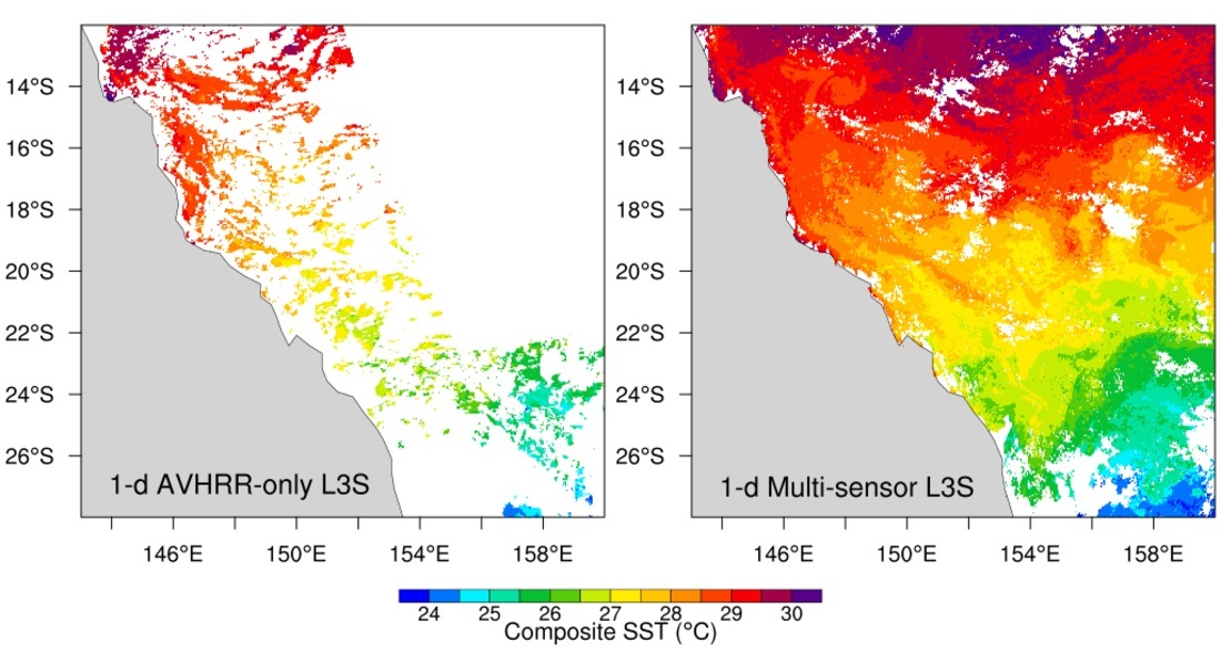
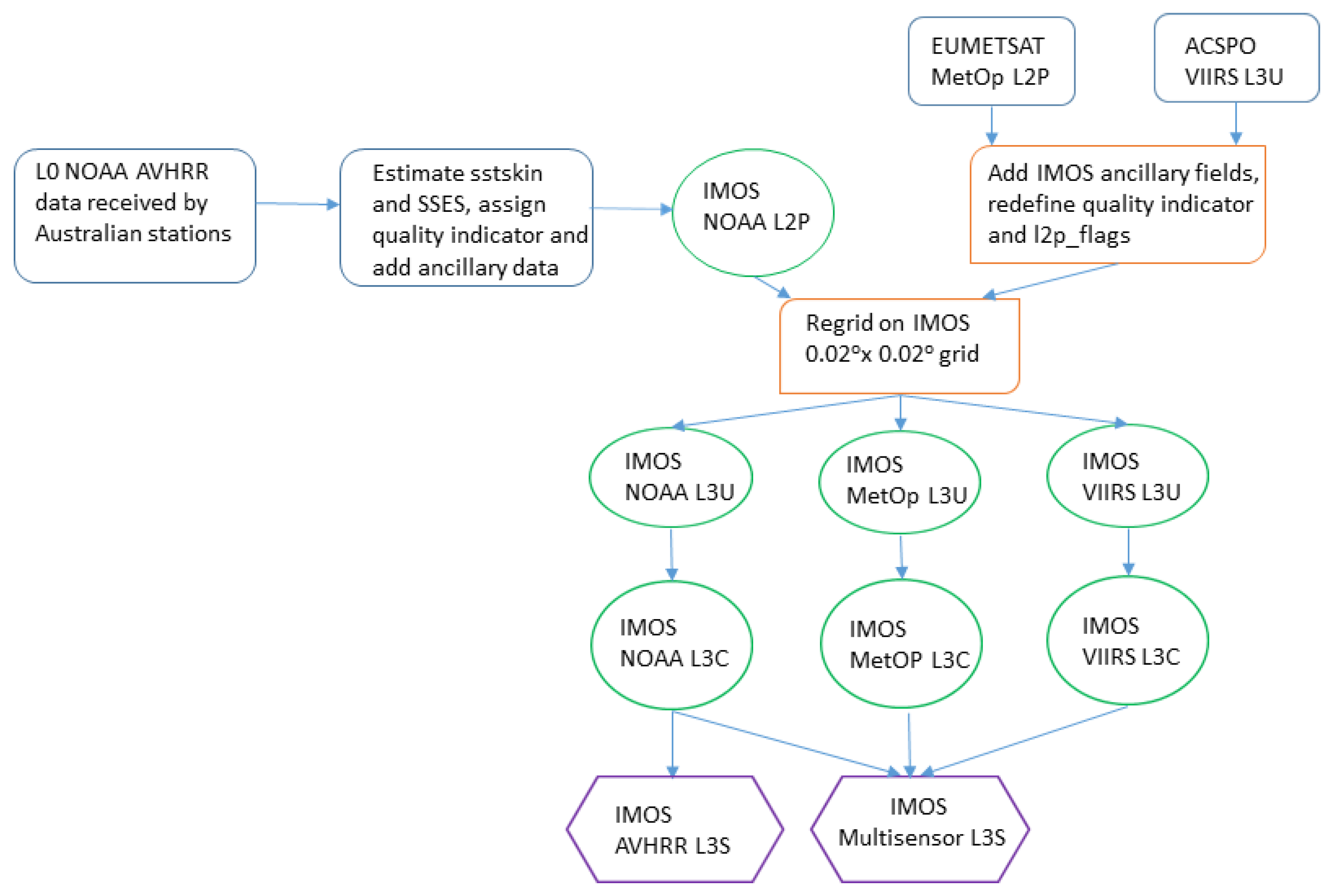
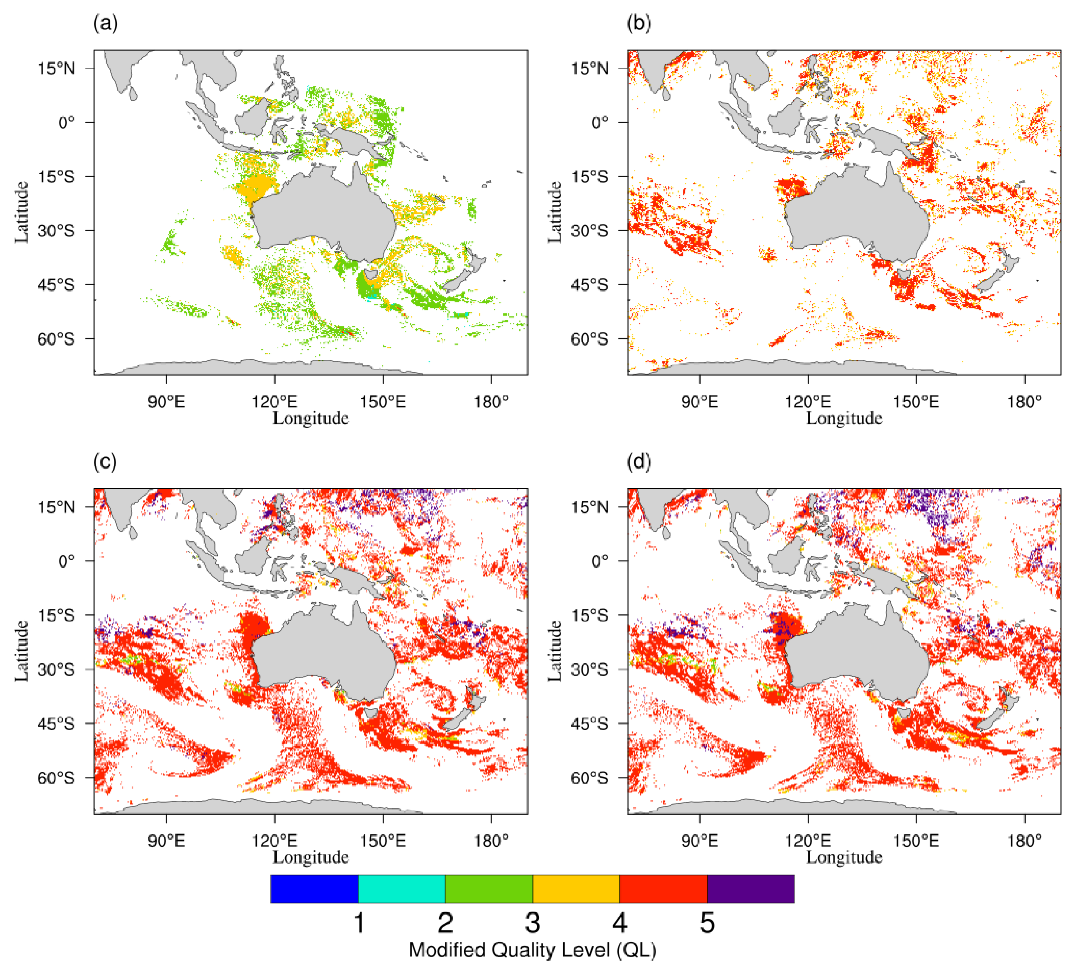
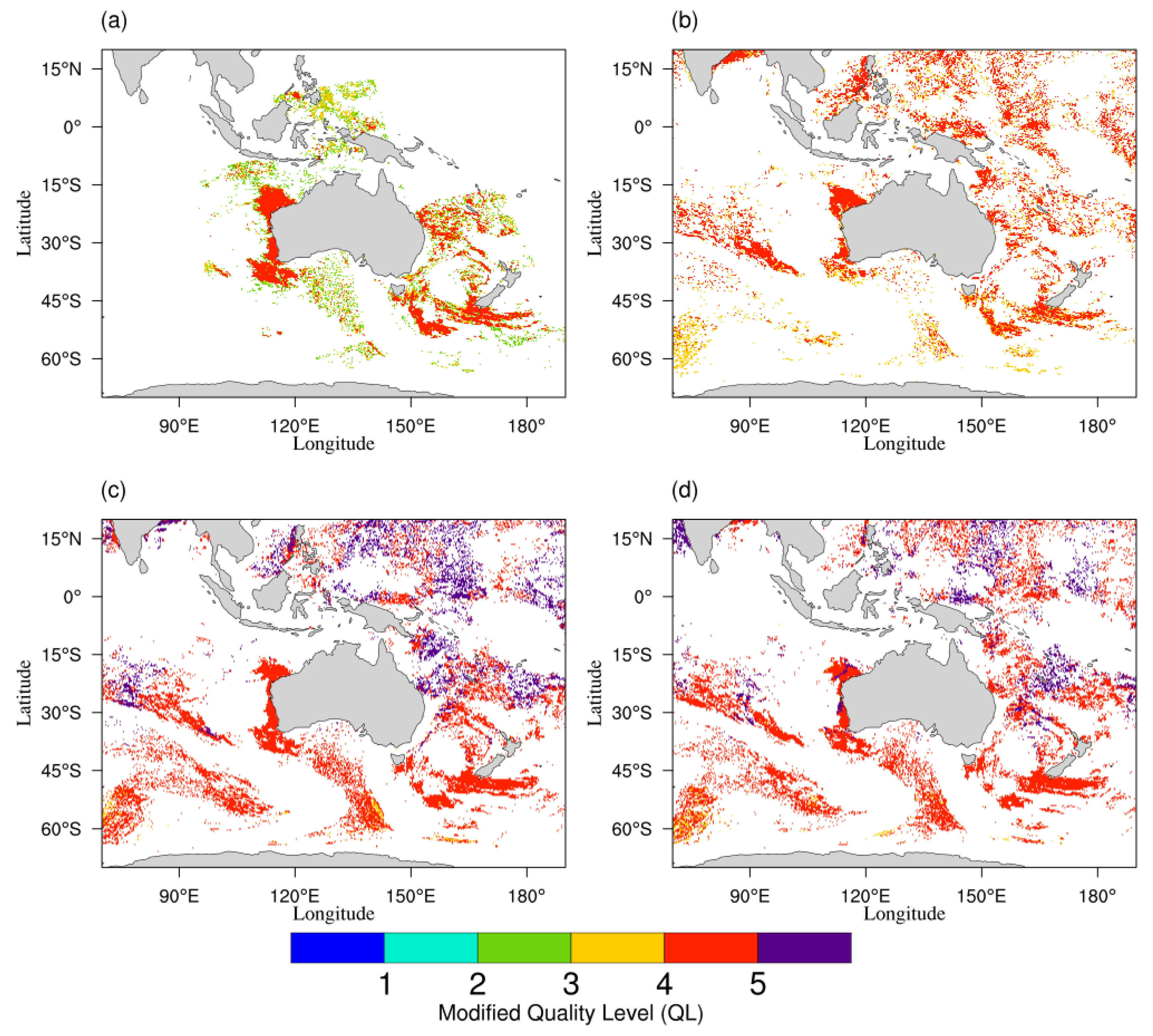
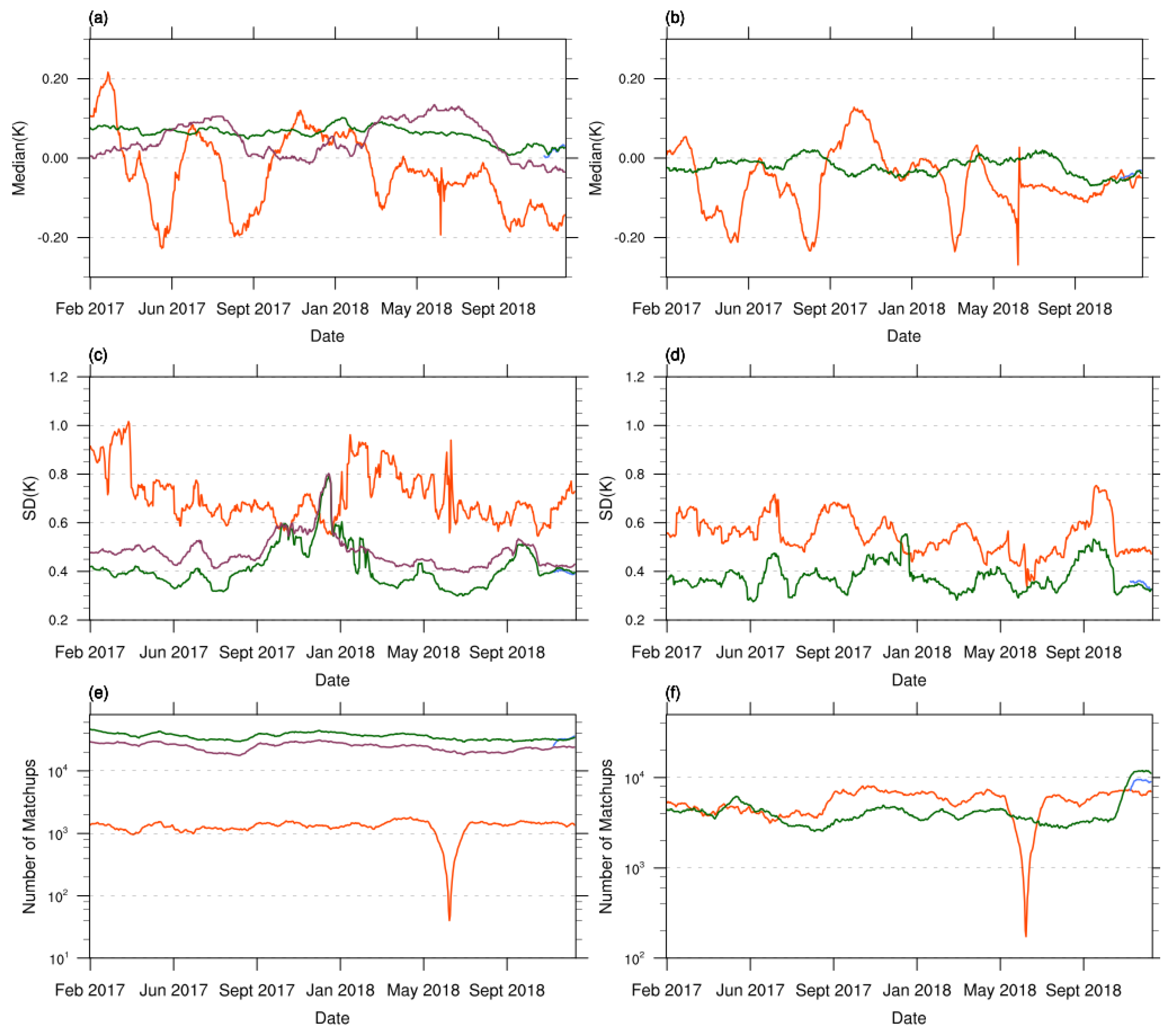
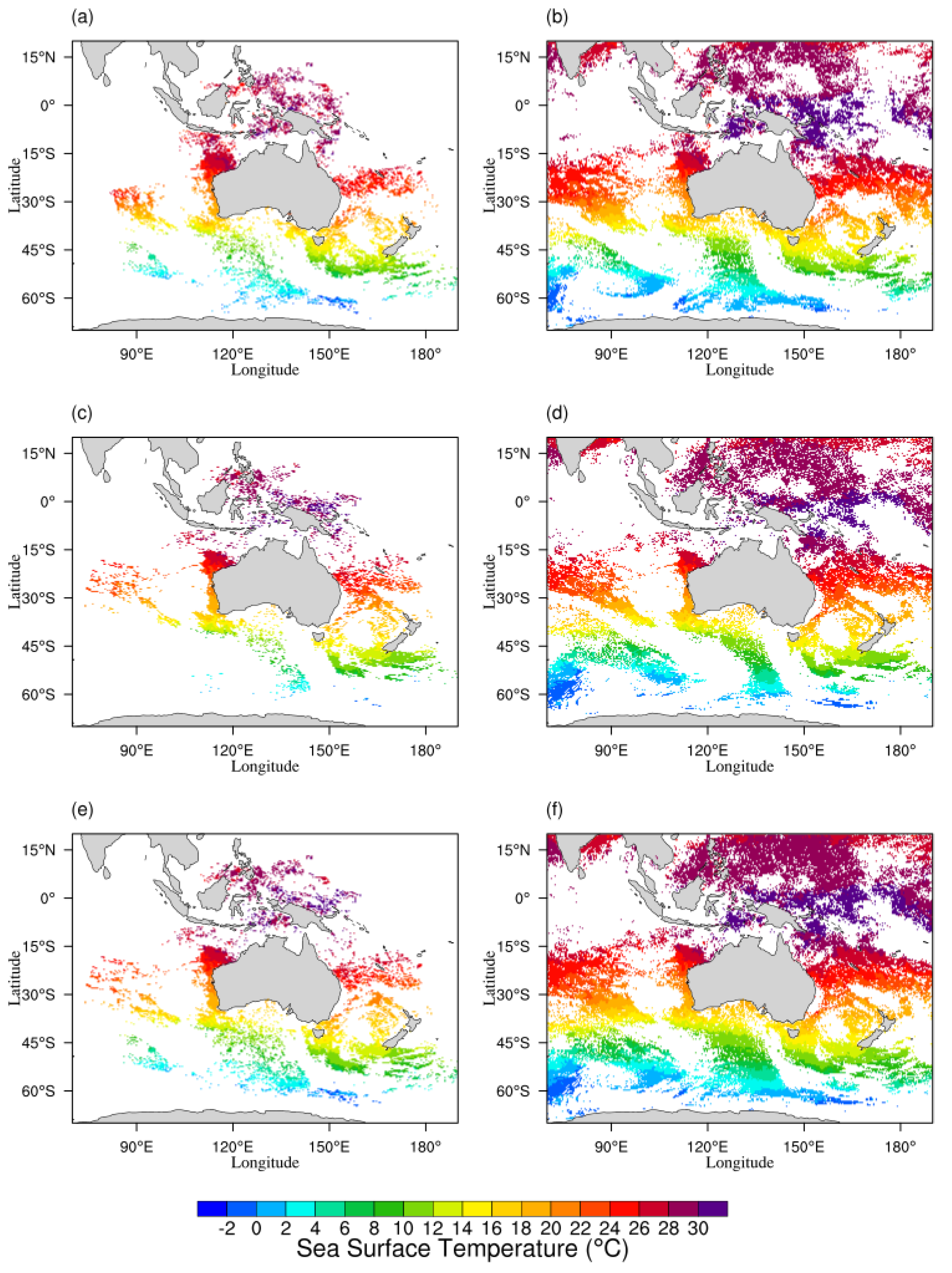
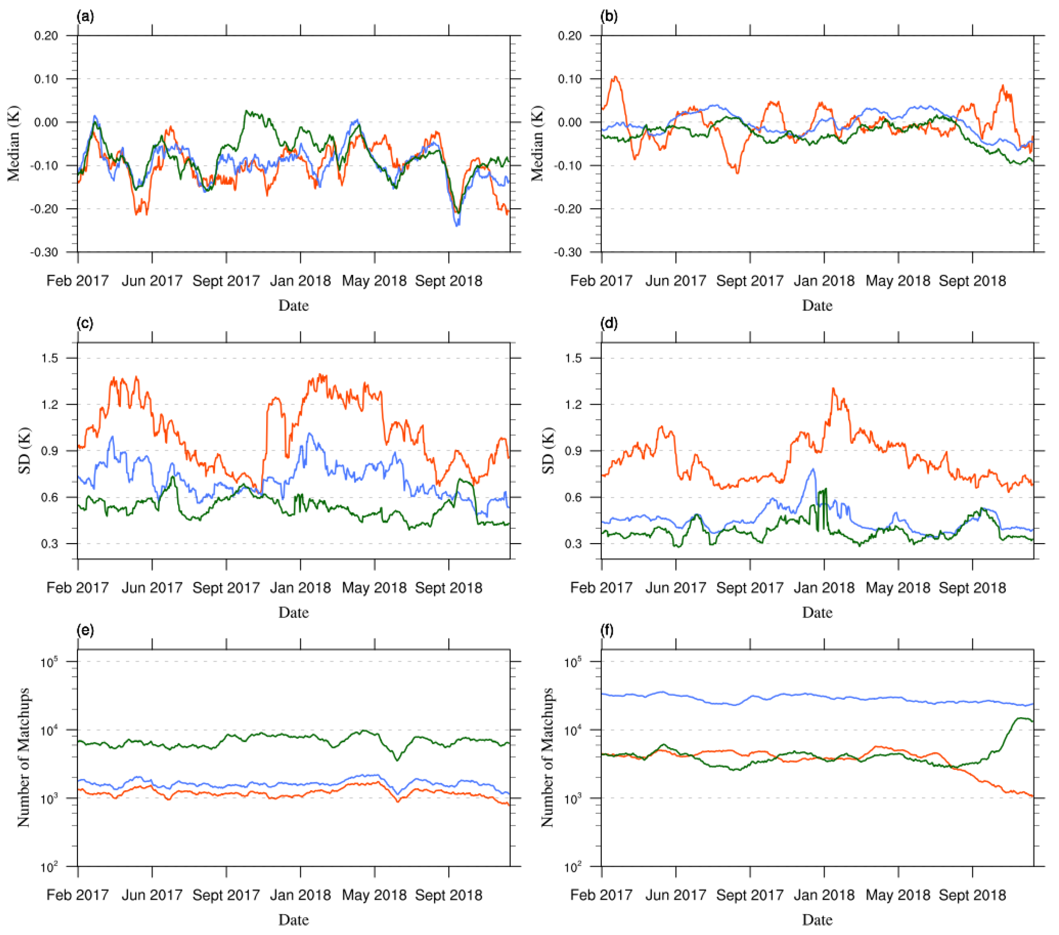
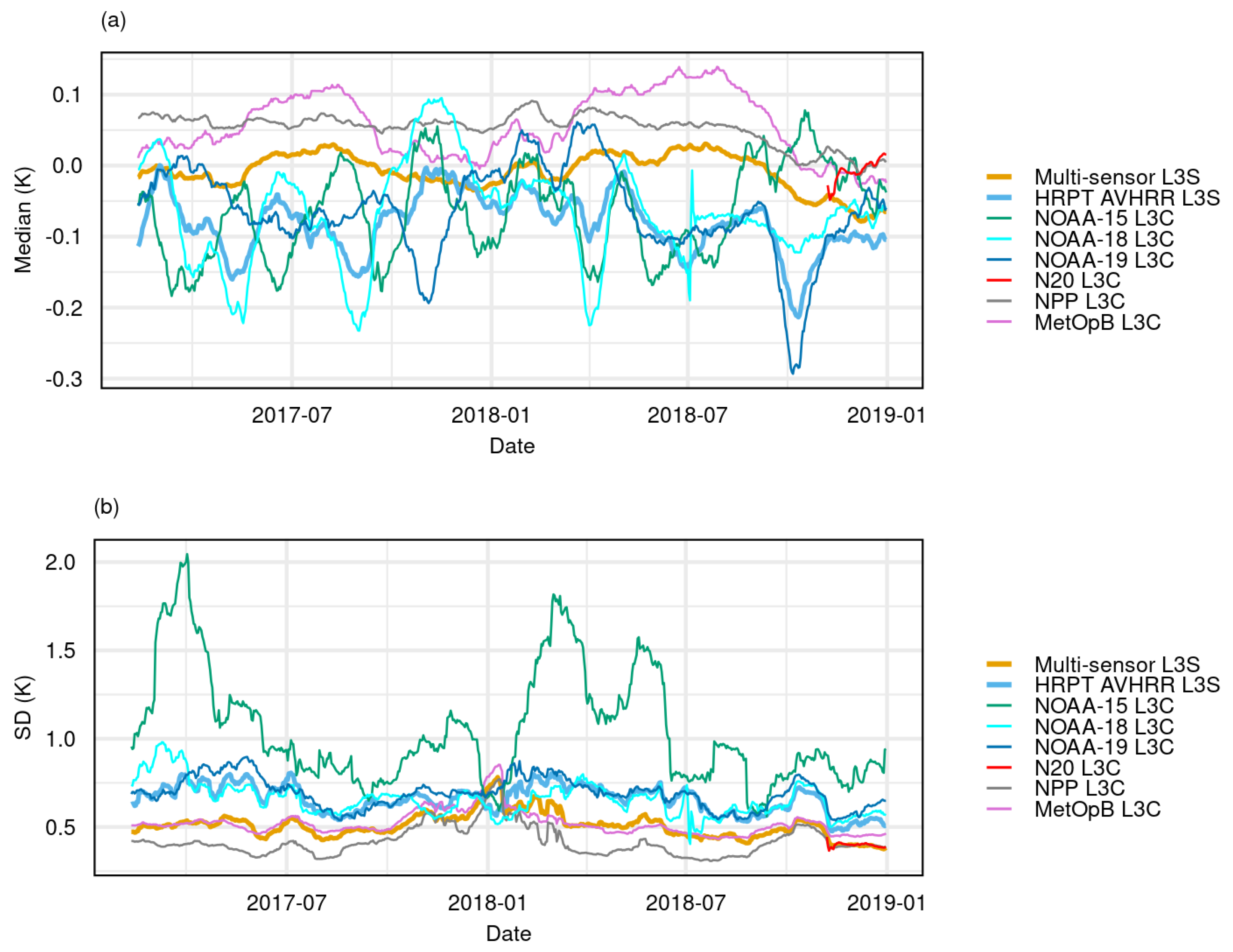
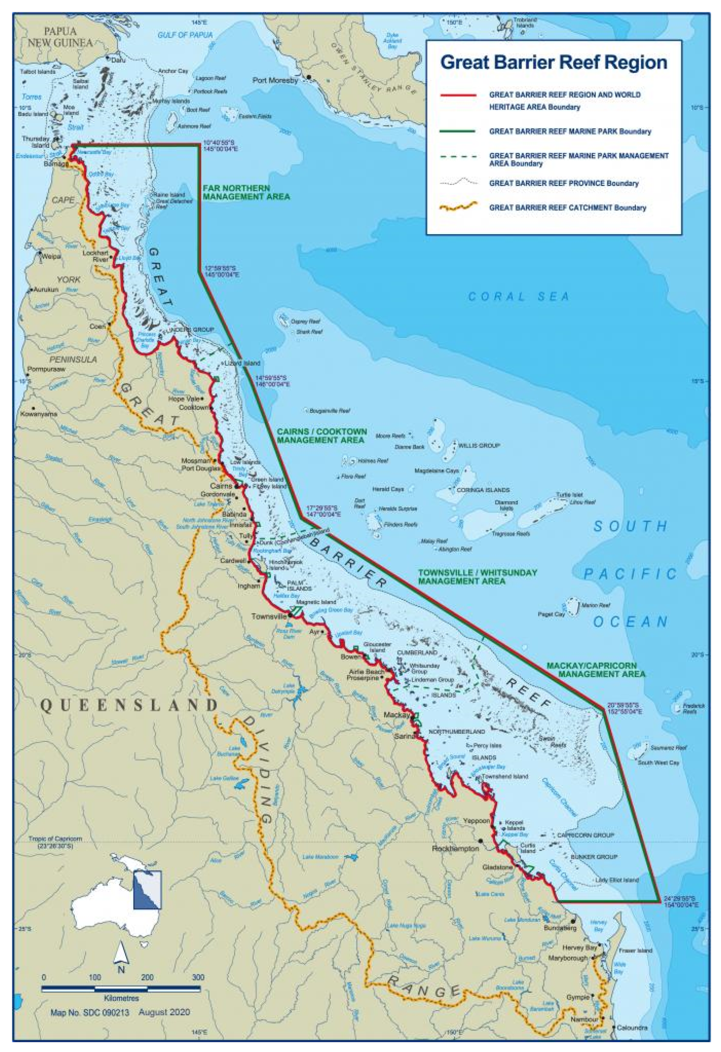
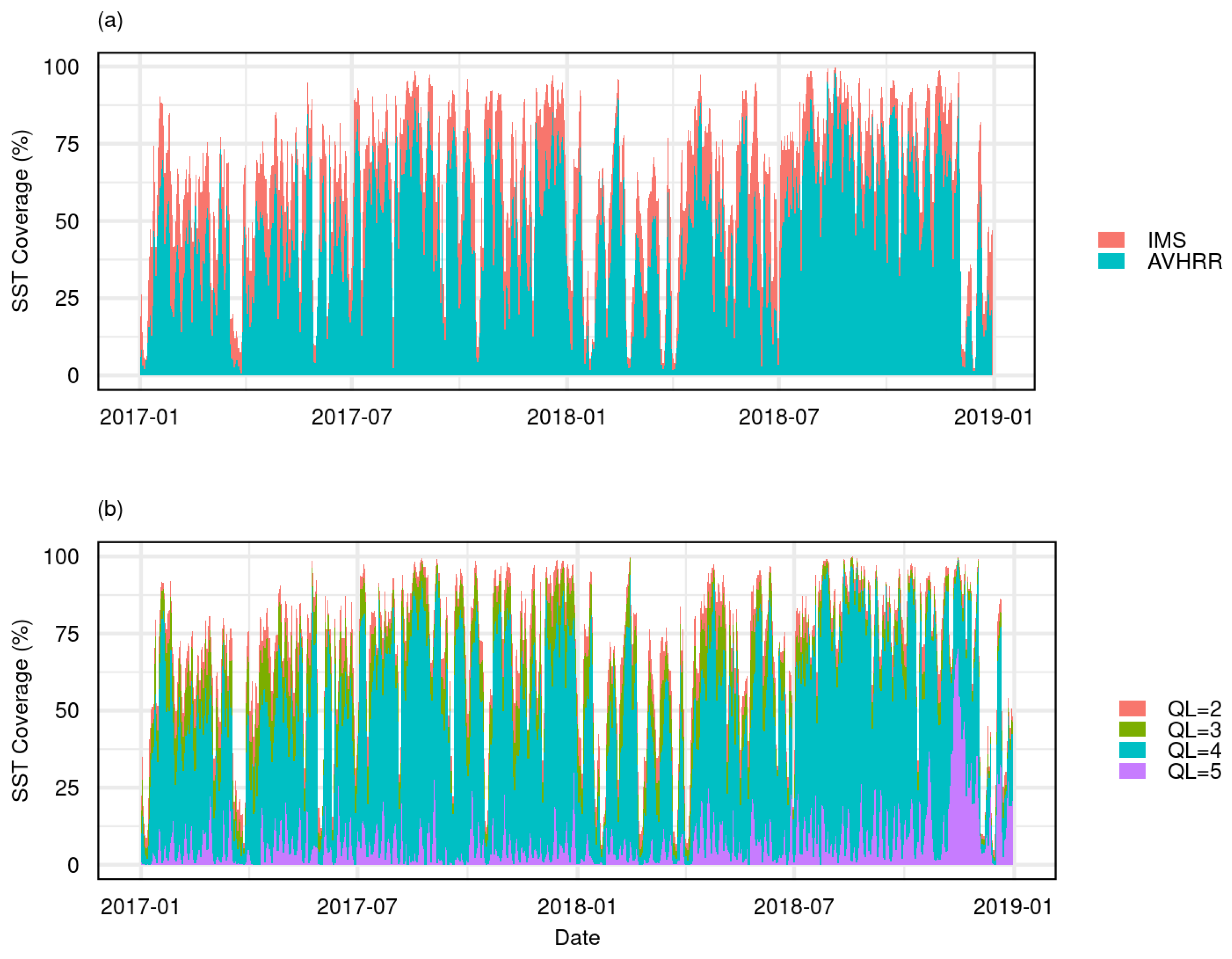
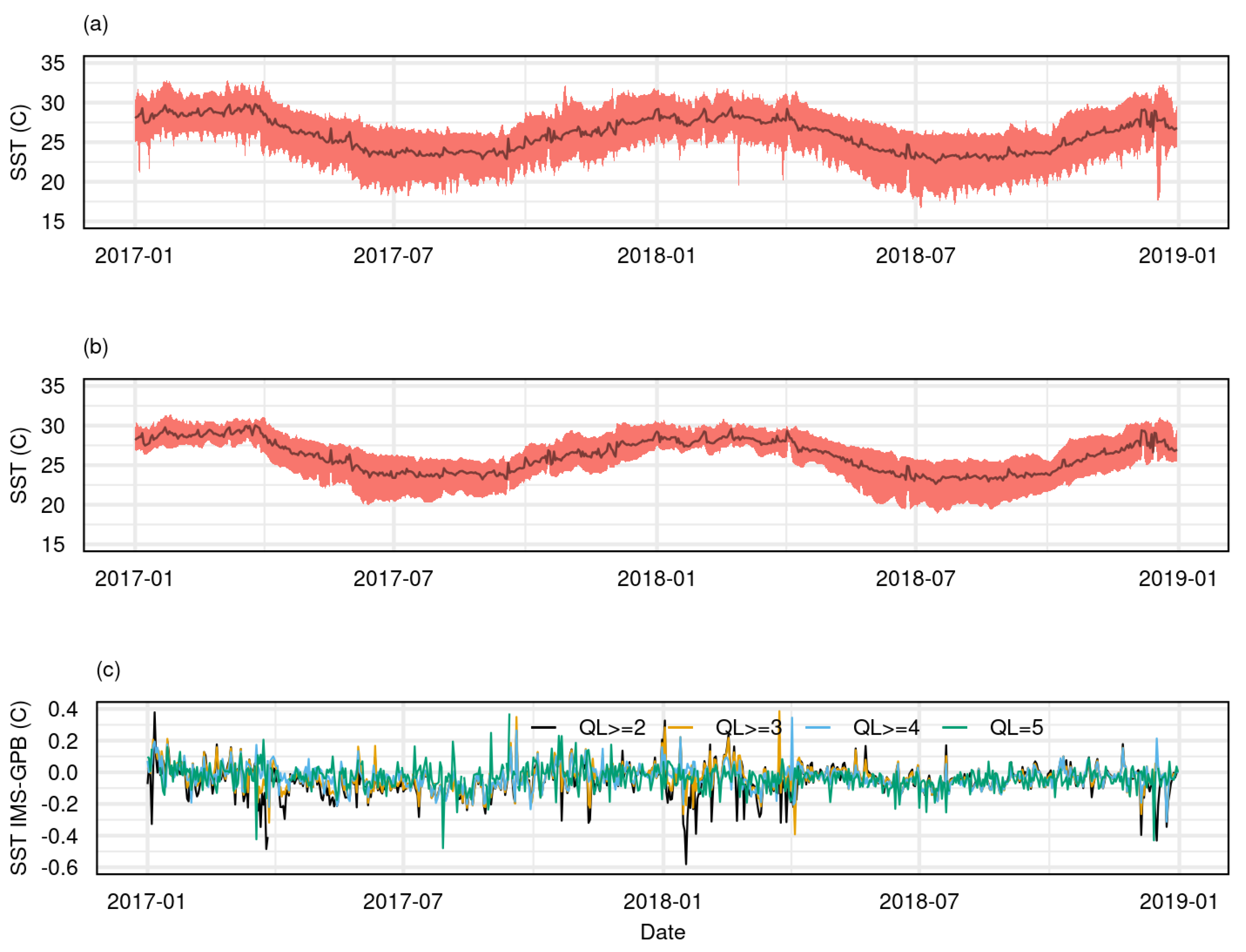
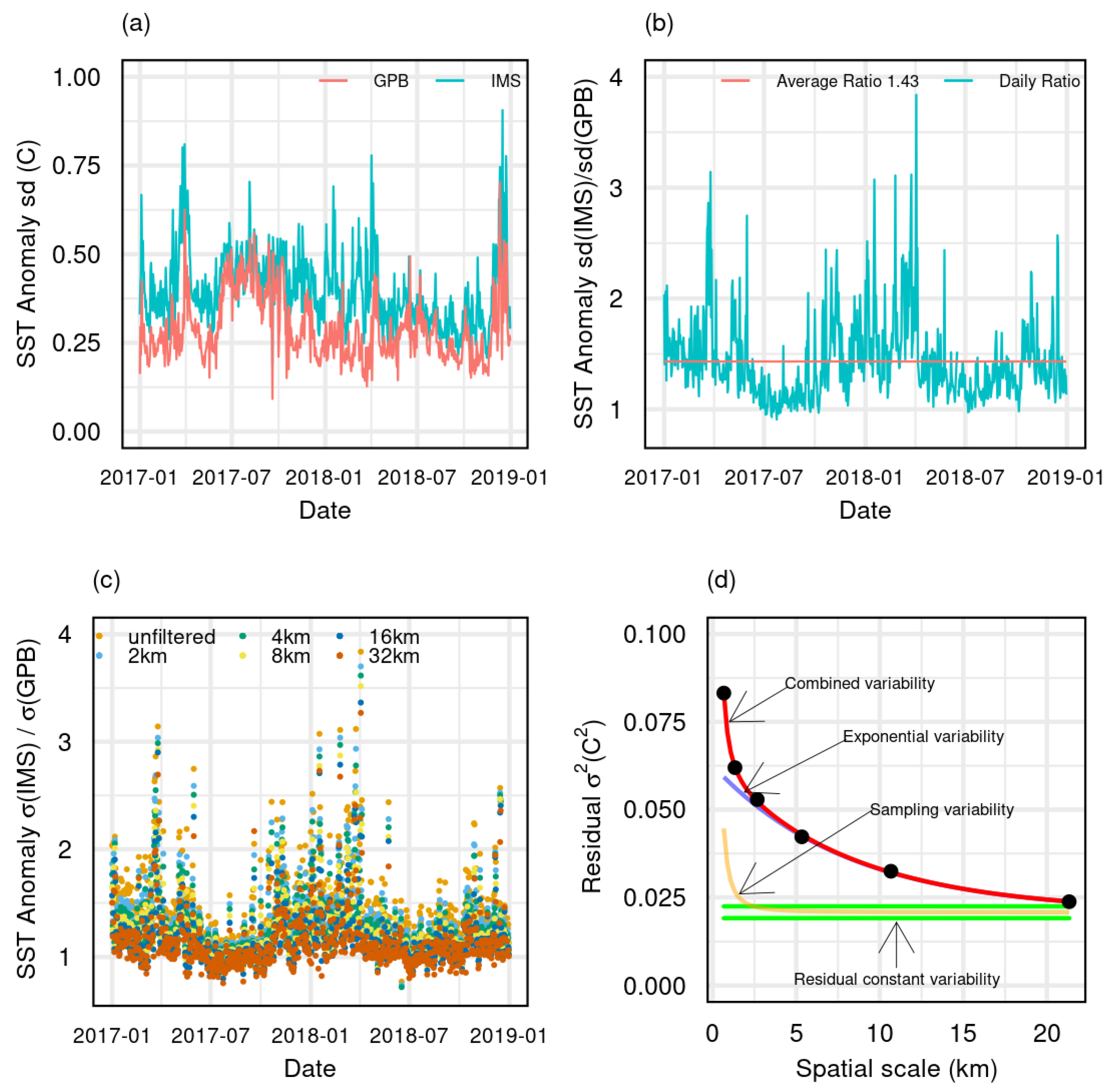
Table 1.
Difference between fv01 and fv02 SST product versions.
| Item | fv01 | fv02 |
|---|---|---|
| SST retrieval | Regression, fixed coefficients tuned over the first 2 years of platform operation. Separate algorithms for day and night with a large number of terms. | Regression, adaptive coefficients tuned over a rolling 2-year window, updated monthly. Separate standard algorithms for day and night as well as a three-channel unified day and night algorithm. |
| SSES generation | Lookup table based on a 60-day rolling window for NOAA-11 to 19 platforms. | Modelled using a one-year rolling window, updated every five days for NOAA 11–19 platforms. |
| Time coverage | 1 January 2019 to present. Coverage may be incomplete over some periods, although the L3S daily composites form a close to complete record. | 2 January 1992 to the end of the most recent batch process. Coverage is complete up to navigation and reception issues and subject to the availability of data from all Australian reception stations, from NOAA-11, 12, 14, 15, 16, 17, 18, 19. |
| Spatial coverage | Includes reception from Australian continental reception stations for NOAA-18,19 and full domain coverage from N20, NPP and MetOp-B satellites. | Includes reception from both continental and Antarctic stations for NOAA-11, 12, 14, 15, 16, 17, 18, 19. Coverage is enhanced over time periods where earlier and later platforms overlap. Spatial coverage has been enhanced in recent years from fully global SST data from N20, NPP, MetOp-A and MetOp-B satellites. |
| Platform coverage | Currently covers NOAA-18, NPP, N20, MetOp-B | NOAA-11, 12, 14, 15, 16, 17, 18, 19, 20, MetOp-A, MetOp-B and NPP. For any given date, all retrievals from the relevant set of active platforms are included in composite L3S files. |
| Fields | sea_surface_temperature, quality_level, sst_dtime, dt_analysis, wind_speed, wind_speed_dtime_from_sst, sea_ice_fraction, sea_ice_fraction_dtime_from_sst, l2p_flags, satellite_zenith_angle, sses_bias, sses_standard_deviation, sses_count | sea_surface_temperature, sea_surface_temperature_day_night, quality_level, sst_dtime, dt_analysis, wind_speed, wind_speed_dtime_from_sst, sea_ice_fraction, sea_ice_fraction_dtime_from_sst, l2p_flags, satellite_zenith_angle, sses_bias, sses_standard_deviation, sses_count, sses_quality_level |
| Metadata | Default, but tends to be inconsistent in some comment fields. | Default |
Table 2.
The parameters used for quality remapping.
| AVHRR | VIIRS | |
|---|---|---|
| −0.2614 | −0.227 | |
| 0.23 | 0.20 |
Table 3.
Dates when platforms were included in the reprocessing of Multi-sensor L3S SSTs.
| Platform | Period |
|---|---|
| NOAA-18 | 1 January 2012 to 31 December 2020 |
| NOAA-19 | 1 January 2012 to 3 September 2018 |
| NPP | 1 March 2012 to 31 December 2020 |
| N20 | 6 June 2018 to 31 December 2020 |
| MetOp-A | 1 January 2012 to 19 January 2016 |
| MetOp-B | 20 January 2016 to 31 December 2020 |
Table 4.
Fitted variability contributions to IMOS Multi-sensor L3S climatology anomalies that were reflected in Geo-Polar Blend L4 climatology anomalies. The linear coefficient is approximated by unity to within 10%.
Table 4.
Fitted variability contributions to IMOS Multi-sensor L3S climatology anomalies that were reflected in Geo-Polar Blend L4 climatology anomalies. The linear coefficient is approximated by unity to within 10%.
| Average Spatial Scale n (km) | Fitted Linear Coefficient | Fitted Constant Coefficient |
|---|---|---|
| 0.67 | 0.94 ± 0.04 | 0.083 ± 0.005 |
| 1.33 | 0.93 ± 0.04 | 0.062 ± 0.004 |
| 2.67 | 0.93 ± 0.04 | 0.053 ± 0.004 |
| 5.33 | 0.92 ± 0.03 | 0.042 ± 0.004 |
| 10.7 | 0.91 ± 0.03 | 0.032 ± 0.003 |
| 21.3 | 0.89 ± 0.03 | 0.024 ± 0.003 |
Publisher’s Note: MDPI stays neutral with regard to jurisdictional claims in published maps and institutional affiliations. |
© 2022 by the authors. Licensee MDPI, Basel, Switzerland. This article is an open access article distributed under the terms and conditions of the Creative Commons Attribution (CC BY) license (https://creativecommons.org/licenses/by/4.0/).
Share and Cite
MDPI and ACS Style
Govekar, P.D.; Griffin, C.; Beggs, H. Multi-Sensor Sea Surface Temperature Products from the Australian Bureau of Meteorology. Remote Sens. 2022, 14, 3785. https://doi.org/10.3390/rs14153785
AMA Style
Govekar PD, Griffin C, Beggs H. Multi-Sensor Sea Surface Temperature Products from the Australian Bureau of Meteorology. Remote Sensing. 2022; 14(15):3785. https://doi.org/10.3390/rs14153785
Chicago/Turabian StyleGovekar, Pallavi Devidas, Christopher Griffin, and Helen Beggs. 2022. "Multi-Sensor Sea Surface Temperature Products from the Australian Bureau of Meteorology" Remote Sensing 14, no. 15: 3785. https://doi.org/10.3390/rs14153785
Note that from the first issue of 2016, this journal uses article numbers instead of page numbers. See further details here.