Article

Effects of Low Temperature on the Relationship between Solar-Induced Chlorophyll Fluorescence and Gross Primary Productivity across Different Plant Function Types

1
Key Laboratory of Digital Earth Science, Aerospace Information Research Institute, Chinese Academy of Sciences, Beijing 100094, China
2
University of Chinese Academy of Sciences, Beijing 100049, China
3
International Research Center of Big Data for Sustainable Development Goals, Beijing 100094, China
*
Author to whom correspondence should be addressed.
Remote Sens. 2022, 14(15), 3716; https://doi.org/10.3390/rs14153716
Submission received: 21 June 2022 / Revised: 28 July 2022 / Accepted: 2 August 2022 / Published: 3 August 2022
(This article belongs to the Collection Feature Paper Special Issue on Forest Remote Sensing)

Abstract

:
Solar-induced chlorophyll fluorescence (SIF) has been recognized as a proxy of gross primary production (GPP) across various terrestrial biomes. However, the effects of low temperature on SIF and GPP among different plant function types (PFTs) have not yet been well-explored. To gain a better understanding of the relationship between SIF and GPP, we investigated the variation in the GPP/SIF ratio in response to low-temperature conditions using satellite and tower-based datasets. Based on the TROPOMI SIF product and FLUXCOM GPP data, we found that the SIF and GPP exhibited consistent seasonal and spatial patterns, while the GPP/SIF ratio differed for different PFTs. The GPP/SIF ratio for forest types was generally higher than 10 gC·d−1·mw−1·nm·sr, whereas the GPP/SIF ratio for grass and crop types was generally lower than 10 gC·d−1·mw−1·nm·sr. In addition, there were noticeable differences in the seasonal pattern of the GPP/SIF ratio between the selected samples that experienced low-temperature stress (below 10 °C, defined as group A) and those that grew under relatively warm conditions (above 10 °C throughout the year, defined as group B). The GPP/SIF ratio for group A generally exhibited a “hump-shaped” seasonal pattern, and that for group B showed a slightly “bowl-shaped” seasonal pattern, which means it is important to consider the effects of temperature on the SIF-GPP relationship. Through linear regression and correlation analysis, we demonstrate that there was a positive correlation between the GPP/SIF ratio and temperature for group A, with a wide temperature range including low-temperature conditions, indicating that, in this case, temperature affected the SIF–GPP relationship; however, for group B—with a temperature higher than 10 °C throughout the year—the GPP/SIF ratio was not consistently affected by temperature. The response of GPP/SIF to low temperature stress was confirmed by tower-based observations at a C3 cropland (C3CRO) site and a boreal evergreen needleleaf forest (BoENF) site. Although the relationship between the GPP/SIF ratio and temperature differed among PFTs, the GPP/SIF ratio decreased under low-temperature conditions for PFTs. Therefore, the GPP/SIF ratio was not constant and was largely influenced by low temperature for different PFTs, thus highlighting the importance of incorporating temperature into SIF-based GPP estimation.

Graphical Abstract

1. Introduction

Large uncertainties occur in the estimation of global terrestrial photosynthesis flux, which is the largest component of the global carbon cycle [1,2]. Solar-induced chlorophyll fluorescence (SIF) is directly related to the light reaction processes of photosynthesis [3], and provides a new way to more accurately map gross primary production (GPP). A large number of studies have found that SIF tracks GPP well at different temporal and spatial scales [4,5,6,7]; however, the SIF–GPP relationship is largely dependent upon the biome and climate [8,9]. How the relationships between SIF and GPP with respect to different plant functional types (PFTs) are influenced by various environmental conditions remains under-explored.
As both SIF and GPP are driven by absorbed photosynthetically active radiation (APAR), the light use efficiency (LUE) model has been successfully used to model the relationship between SIF and GPP [10,11]. Indeed, a large number of studies have found that the SIF presents a strong linear relationship with GPP at large temporal and spatial scales [12,13,14]. However, it has been shown that SIF is more strongly related to APAR than to photosynthesis [15,16], and the relationship between SIF and GPP is modulated by other processes [17,18,19]. The energy absorbed by chlorophyll molecules can be dissipated through photochemical quenching (PQ), non-photochemical quenching (NPQ), and SIF at the leaf level [20]. SIF is directly related to the light reaction, whereas the potential mechanistic link between SIF and the linear electron transfer rate needed for carboxylation processes is the key point linking SIF to GPP [3,21]. The differences in carbon reaction between C3 and C4 species may result in the different slopes of SIF and GPP [7,22]. At the canopy level, the canopy-observed SIF is only part of the total SIF emitted from the chlorophyll molecules, due to scattering and reabsorption effects [18,23,24,25]. The canopy structure and chlorophyll content also affect the SIF–GPP relationship in some aspects [26,27,28,29,30]. Therefore, these interactions make the SIF–GPP relationship complex [2,31]. The responses of SIF and GPP to varying environmental conditions across ecosystems remain unknown, resulting in uncertainties in the estimation of global GPP based on SIF.
The effects of environmental conditions on the relationship between SIF and GPP have become a state-of-the-art topic. As SIF emitted from photosystem II (PS II) is directly linked to the photosynthetic activity, it is strongly affected by environmental conditions [7,32]. The proportion of energy allocated to each energy-dissipated pathway will vary under different environmental conditions [33,34]. In addition, the differences in light and carbon reactions in response to changing environmental conditions will also affect the SIF–GPP relationship [35,36]. A large number of studies have reported that SIF and GPP respond differently to light intensity [21,37,38] at both leaf and canopy levels, where the ratio of GPP to SIF decreased with increasing light intensity. Although SIF can partly track the down-regulation of GPP under drought conditions [39,40], drought stress also affects the SIF–GPP relationship [41,42]. The incongruity of light and carbon reactions and the complex energy distribution under stress conditions may contribute to the different sensitivities of SIF and GPP in response to drought stress [3,21].
Recent studies have begun to explore the responses of SIF and GPP to temperature [40,43]. Song et al. [44] found that satellite SIF allowed for early detection of the response of winter wheat to heat stress, and could provide a larger physiology-related stress response than APAR and traditional vegetation indices (e.g., the enhanced vegetation index; EVI) during heatwave events. Kimm et al. [45] quantified the effects of high-temperature stress on canopy photosynthesis and demonstrated that SIF responded sensitively to the physiological down-regulation of GPP based on a high-temperature experiment in a soybean field. Kim et al. [46] explored the relationship between SIF and GPP in a temperate evergreen needleleaf forest during the fall transition, and they found that LUE reached saturation at high air temperatures, whereas the chlorophyll fluorescence yield (ФF) did not saturate. In addition, Magney et al. [9] reported that both SIF and GPP in a boreal evergreen needle forest (BoENF) tracked with each other in a consistent, dynamic fashion in response to low temperature. Furthermore, they pointed out that, compared to traditional vegetation-index-based methods, SIF—being directly related to needle physiology—has the unique ability to capture GPP seasonality. It should be pointed out that the photochemistry quantum efficiency of PS II is not significantly affected by temperature at low light intensity, and that the temperature has a direct effect on the kinetics of enzymes involved in carbon reactions [47]. Therefore, different light, moisture, or temperature conditions likely affect the SIF–GPP relationship to some degree [3].
Temperature has large effect on photosynthesis, and the effects of temperature on photosynthetic activities vary with the plant species [35,48]. The response of photosynthesis to low-growth-temperature conditions depends largely on the original distribution of the species [49]. Plants can be classified as species adapted to cold environmental conditions and species adapted to warm conditions (e.g., tropical or sub-tropical conditions). Some studies have reported that there is a striking difference between those two groups, considering the effect of low temperature on photoinhibition [50,51]. However, to date, the influence of low temperature on the SIF–GPP relationship for different PFTs has not been well-explored [9,21,52].
Launched on 13 October 2017, the TROPOspheric Monitoring Instrument (TROPOMI) on board the Copernicus Sentinel-5 Precursor satellite (S5P) is the first of the atmospheric composition Sentinels, which has relatively fine temporal and spatial resolution [25,53]. Due to its relatively fine resolution and its ability to take more spatially continuous measurements than other SIF-related satellites, the SIF retrieved from TROPOMI has been widely used to explore the seasonal variations in GPP, enhancing its ability to detect environmental stresses [14,54]. Tower-based continuous observations also provide reliable data for the study of diurnal and seasonal changes in SIF, as well as its relationship with GPP under various environmental conditions [7,9,55,56,57]. Therefore, continuous reliable satellite and tower-based data were considered to support our study regarding the effects of temperature on the SIF–GPP relationship for different PFTs.
In this study, the influences of low temperature on the SIF–GPP relationship were assessed using both satellite and tower-based observations. We investigated the relationship between the GPP/SIF ratio and temperature for different PFTs in order to address the following specific issues: (1) What are the differences in the SIF–GPP relationship under different growth temperature conditions? (2) How do these relationships vary between PFTs? and (3) What is the potential influence of low temperatures on the GPP/SIF ratio?

2. Materials and Methods

2.1. TROPOMI SIF

The single payload of TROPOMI mounted on the Sentinel 5 Precursor (S-5P) satellite has a near-polar, sun-synchronous orbit. TROPOMI SIF has a repeat cycle of 16 days in the nadir direction, and its equatorial overpass time is ~13:30 local time [54], similar to that of OCO-2. Compared to OCO-2, the wider swath (~2600 km) and higher number of observations per second of TROPOMI make it feasible to generate near-daily gridded SIF products at relatively fine temporal and spatial resolution [25]. Recently, TROPOMI SIF has successfully been retrieved using a data-driven approach based on principal component analysis in the atmospheric windows of 735–758 nm and 743–758 nm for the far-red SIF [53].
In this study, we used the ungirded TROPOMI far-red SIF (743–758 nm) from February 2018 to December 2020 (https://s5p-troposif.noveltis.fr/data-access/, assessed on 1 December 2021). In order to eliminate the influences of different solar illumination geometry on the SIF magnitude, by applying a day-length correction factor, the instantaneous TROPOMI SIF was converted to a daily average [58]. In addition, SIF observations with a cloud fraction higher than 0.2, view zenith angle (VZA) over 15°, and solar zenith angle (SZA) larger than 70° were excluded in order to reduce the effects of clouds and the observational geometry [19,59,60]. Finally, the filtered SIFs were averaged at 0.25° × 0.25° spatial resolution and 8-day temporal resolution (Figure 1b).

2.2. FLUXCOM GPP

Based on machine learning, the CO2 flux measurements from the FLUXNET eddy covariance towers, merged with remote sensing and meteorological data, have successfully been used to produce global gridded carbon flux data (FLUXCOM GPP) [61]. The FLUXCOM GPP includes two datasets: (1) one at 0.0833° resolution, using Moderate Resolution Imaging Spectroradiometer (MODIS) remote sensing data (abbreviated as RS); and (2) another at 0.5° resolution, using remote sensing and meteorological data (abbreviated as RS + METEO) [62,63]. The dataset is available at ftp://ftp.bgc-jena.mpg.de/pub/outgoing/FluxCom (assessed on 1 December 2021). In this study, we used the FLUXCOM GPP global product (RS_V006) at a temporal resolution of 8 days and a spatial resolution of 0.0833°, the good performance of which for carbon fluxes has been revealed by cross-validation [64]. To match the SIF dataset, we obtained the FLUXCOM (RS_V006) GPP from February 2018 to December 2020 and resampled it to 0.25° × 0.25° (Figure 1a).

2.3. ERA5 Re-Analysis Dataset

Using the laws of physics to combine model data with observations from across the world, the European Centre for Medium-Range Weather Forecasts (ECMWF) generates a global complete and consistent re-analysis dataset. In this study, we used the fifth generation of the European Re-analysis dataset (ERA5), which has been proven to be relatively reliable for the analysis of land changes [65,66]. ERA5 provides hourly estimates at a spatial resolution of 0.25 degrees for a large number of land-surface quantities.
The surface temperature of air at 2 m (Ta), measured in kelvin (K), can be converted to degrees Celsius (°C) by subtracting 273.15 [67]. The daily mean Ta (in °C) was obtained by averaging the temperature over 24 h. Similarly, we obtained the daily mean dewpoint temperature (Tdew; in °C). The vapor pressure deficit (VPD; in kPa) can be calculated by converting Ta and Tdew to the vapor pressure [68]. We used the VPD for the indication of drought conditions. The accumulated solar shortwave radiation (J·m−2) reaching a horizontal plane at the surface of the earth should be divided by the accumulation period, expressed in seconds, and then multiplied by 0.46 to obtain the daily averaged PAR (W·m−2) [69]. The PAR, measured in units of energy (W·m−2), was then converted to units of matter (umol·m−2·s−1). Similarly, we averaged the climate environmental variables over 8 days to obtain a dataset with 8-day temporal resolution (Figure 2b).

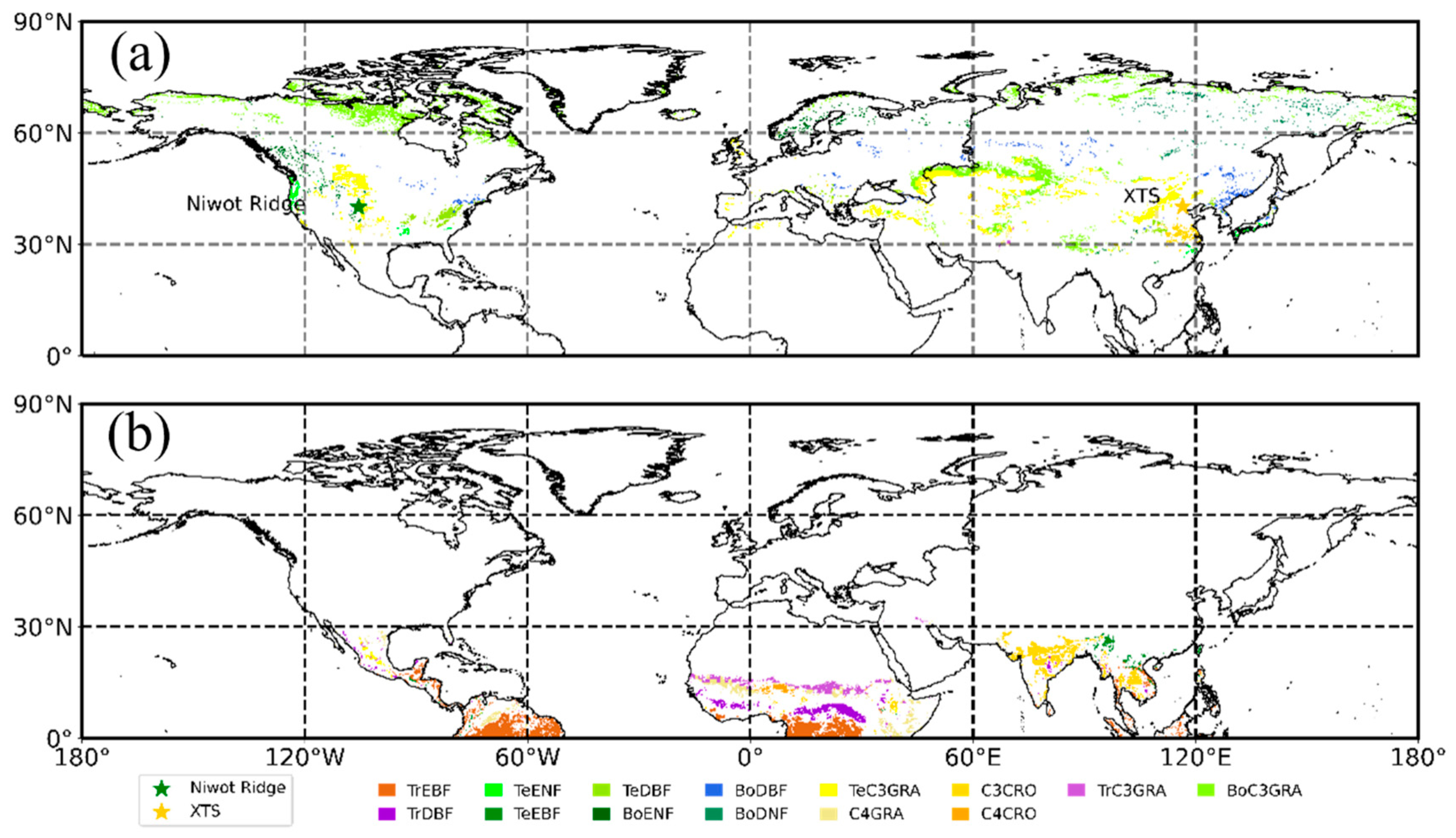
2.4. PFTs Map and Selection of Homogeneous Samples

To better understand the response of the GPP/SIF ratio to temperature under different PFTs, we used a vegetation map including 14 vegetated PFTs (Figure 2a). The vegetation map was produced by the European Space Agency (ESA) Climate Change Initiative (CCI) Land-Cover (LC) products, Land-Use Harmonization (LUH2), and an additional partitioning C3/C4 vegetation map using the cross-walking approach [70,71].
The selection of homogeneous samples was performed on the CCI PFTs map, with a spatial resolution of 0.25° × 0.25° for each PFT. To ensure sufficient PFT homogeneity and sufficient temporal sampling of the pixels, the selected samples had to satisfy prescribed selection criteria. The clustering approach was used to select samples for each PFT, referring the study of Bacour et al. [8]. Only pixels with (1) a fraction of dominant PFT over 50% (Figure 2a), (2) distribution in the North Hemisphere, and (3) at least eight TROPOMI SIF observations for the year 2020 were selected. The reason why only samples distributed in the Northern Hemisphere were selected was to avoid the seasonal pattern differences between the Northern and Southern Hemispheres; additionally, the samples distributed in the Northern Hemisphere contained most vegetation types.
In addition, as some PFTs were distributed in regions with different temperature conditions, some of the selected samples of each PFT experienced low-temperature conditions, while others grew in relatively warm conditions. Some studies have reported that most photosynthetic activities are limited at temperatures below the “biological zero”, which is defined as the minimum development temperature and is generally recognized to be in the range of 5–10 °C, depending on the species and climate [72,73,74]. In this study, we recognized temperatures below 10 °C as low-temperature conditions. Therefore, the selected samples of each PFT were further classified into two groups: one group experienced low-temperature conditions (below 10 °C) and had more than 8 observations below 10 °C in the year 2020 (defined as group A) (Figure 3a); the other group grew under temperatures above 10 °C throughout the year 2020 (defined as group B) (Figure 3b). Finally, the spatial distribution of groups A and B for each PFT can be seen in Figure 3. The number of selected homogeneous samples for each PFT can be found in Table 1; it should be noted that not all PFTs belonged to both group A and B.

2.5. Tower-Based Observations

The relationship between GPP/SIF and temperature was also examined using tower-based observations of two overwintering plants, including winter wheat (C3CRO) and boreal evergreen needleleaf forest (BoENF).
The tower-based observations of winter wheat were conducted at the Xiao Tangshan Farm (XTS, 40.18°N, 116.44°E; Figure 3a) in north Beijing, China [7]. The canopy SIF and GPP measurements at the XTS site covered the period from September 2020 to June 2021. The dataset of a subalpine conifer forest at Niwot Ridge (40.03°N, 105.55°W) covered the period from 21 June 2017 to 29 June 2018 (Table 2). Therefore, both the XTS and Niwot Ridge sites experienced low-temperature conditions during the over-wintering period. Similar to the SIF retrieval method used by Magney et al. [9], SIF retrievals at XTS were also conducted using the differential optical absorption spectroscopy (DOAS) method at the far-red band. The fluxes of GPP and ecosystem respiration (Re) were partitioned from net ecosystem exchange (NEE) based on night-time partitioning algorithms (Reichstein et al., 2005). For more details about the spectrometric instrument used, please refer to the studies of Du et al. [75] and Grossman et al. [76].

2.6. Data Analysis

Negative SIF values were excluded from the analysis, as well as the SIF values greater than 1.5 W·m−2·nm−1·sr−1. Measurements outside the range μ ± 3σ (where μ and σ are the mean and standard deviation, respectively) were also not considered. The filtered data were classified into 14 PFTs, and each PFT was grouped into subset A or subset B, based on the selection criteria described in Section 2.4. Linear regression analysis was conducted to explore the relationship between SIF and GPP in response to temperature. In addition, in order to remove the potential influence of other environmental variables (e.g., PAR and VPD), we conducted partial correlation analysis to study the influence of temperature conditions on the GPP/SIF ratio.

3. Results

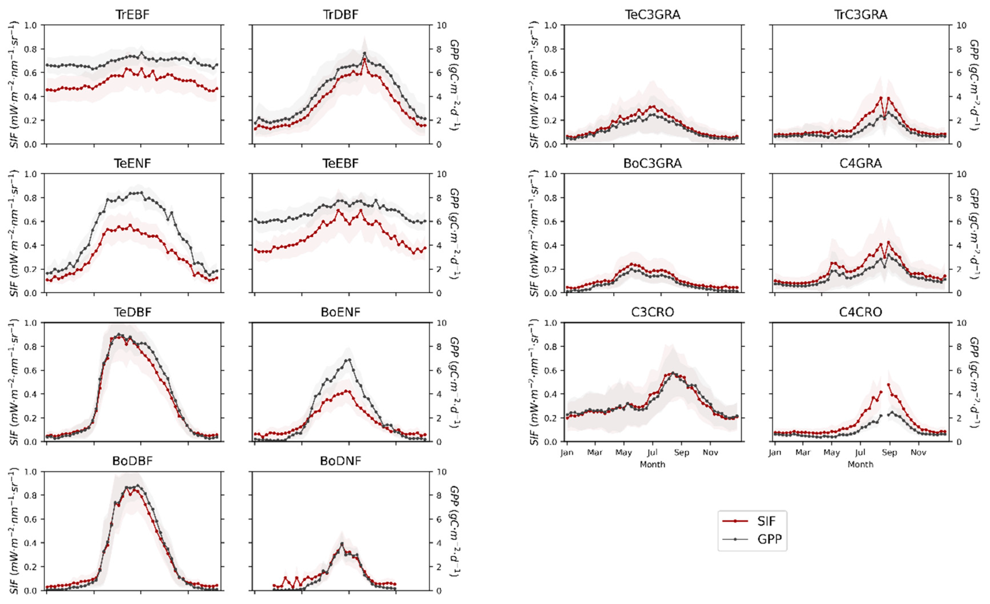
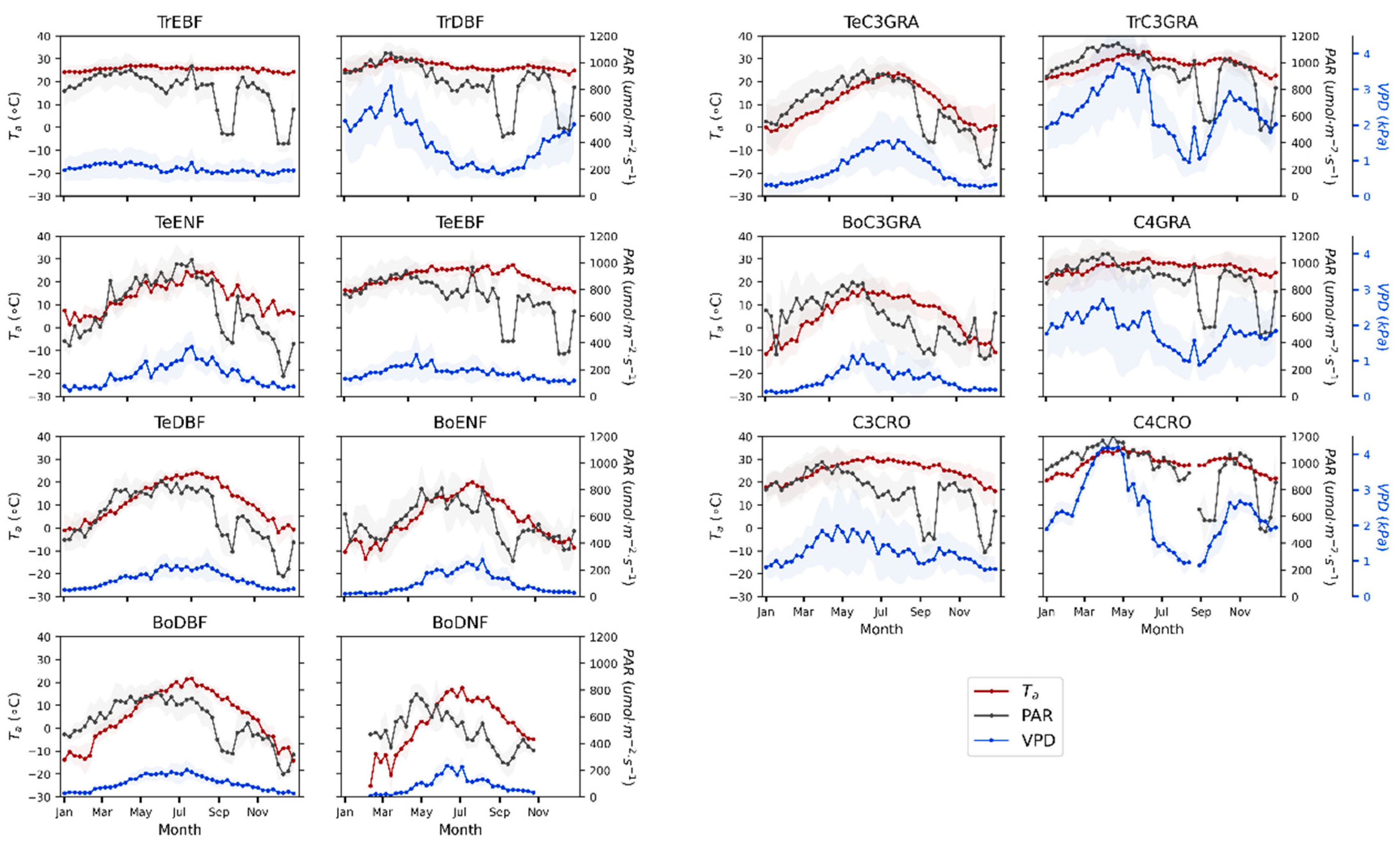
3.1. Seasonal Patterns of SIF and GPP across PFTs

From Figure 1, we can see that the spatial variation in SIF was consistent with that of GPP, indicating that SIF has the ability to track GPP at the global scale. In addition, the seasonal patterns of SIF and GPP for different PFTs are important for our understanding of the responses of SIF and GPP to temperature.
It can be seen that SIF had a similar seasonal pattern to GPP for each PFT in the Northern Hemisphere (Figure 4). Although SIF tracked the GPP well for different PFTs, the seasonal patterns of SIF and GPP were largely influenced by environmental conditions. For tropical regions, although TrEBF, TrDBF, and TrC3GRA grew under relatively comfortable temperature conditions (Figure 5), SIF and GPP of TrEBF did not exhibit an obvious seasonal change, compared to that of TrDBF and TrC3GRA. The seasonal variations in SIF and GPP for TrDBF and TrC3GRA may have been largely influenced by the VPD, which varied with the change from dry to wet seasons (Figure 5). Compared to TeENF and TeDBF, SIF and GPP for TeEBF did not show a more intense seasonal pattern, as air temperature and PAR for TeEBF did not significantly change during the growing period (Figure 5). For Boreal regions, BoENF, BoDBF, BoDNF, and BoC3GRA generally experienced low-temperature stress (less than 10 °C; Table 1). We can see that the magnitude of SIF and GPP for BoENF, BoDBF, BoDNF, and BoC3GRA decreased when the temperature decreased during the over-wintering period. As different PFTs have different growth temperature conditions, the seasonal variations in SIF and GPP for different PFTs responded differently to temperature.
In addition, due to their varying geographical distribution, some PFTs were not only distributed at places where relatively warm conditions prevailed throughout the year, but also in places where low-temperature stress could occur. For example, C3CRO distributed at low latitudes generally grew under relatively warm conditions, while those distributed at high latitudes experienced low-temperature stress (Figure 3). These data provide us with a chance to study the variations in SIF and GPP in response to temperature.

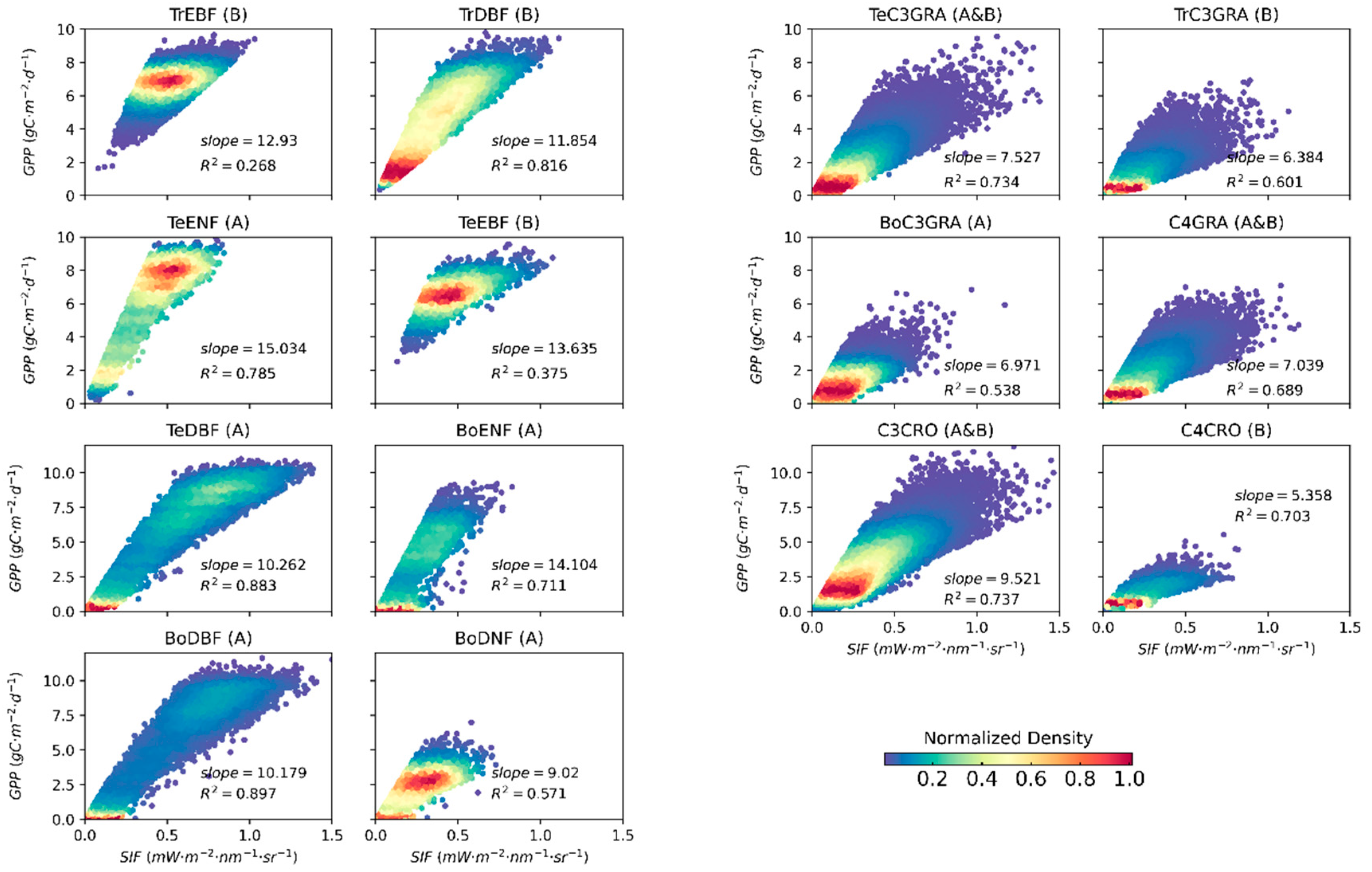
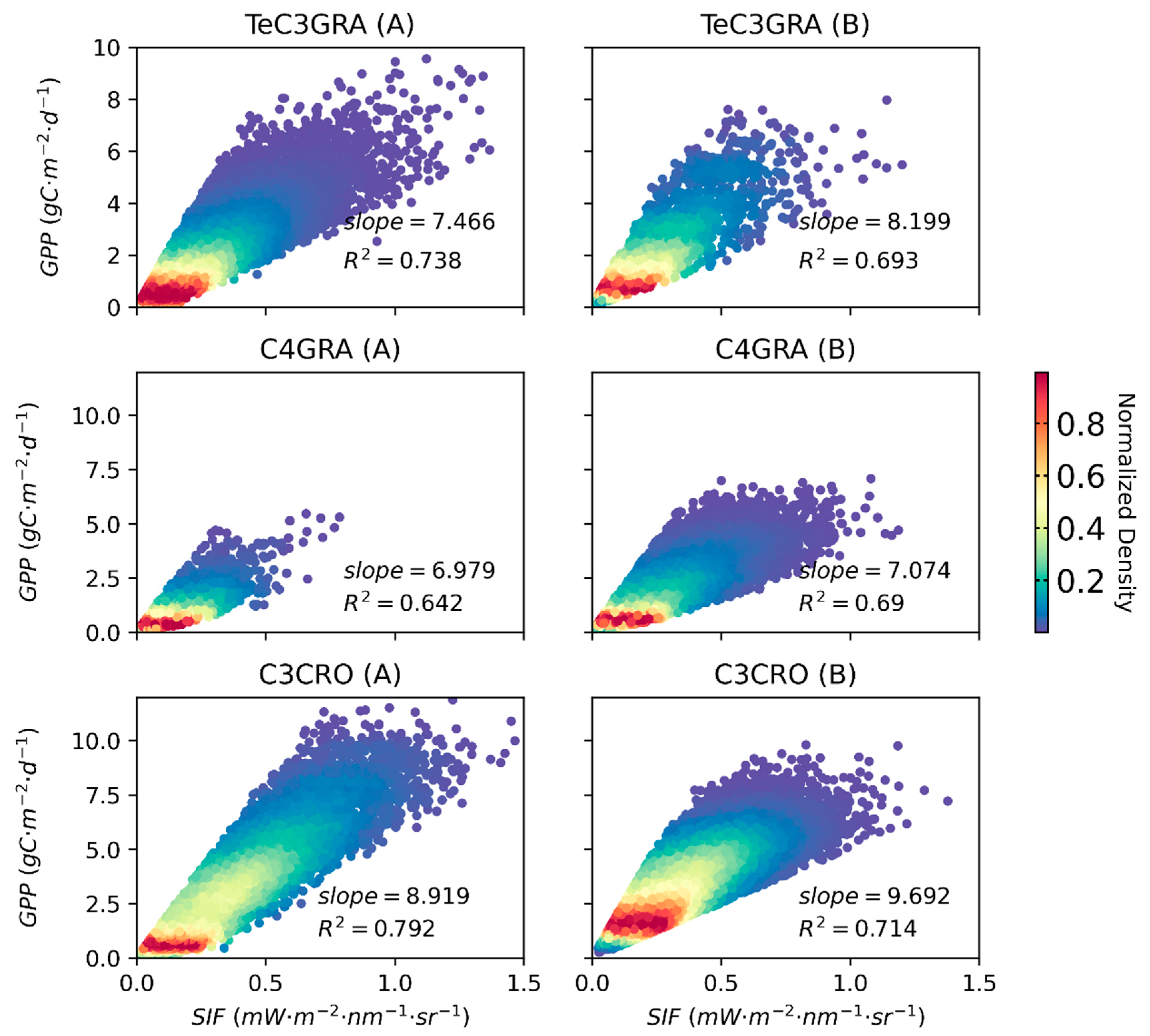
3.2. Relationships between Satellite-Based SIF and GPP for Different PFTs

To evaluate the performance of SIF, in terms of estimating GPP for different PFTs, we compared the relationships between TROPOMI SIF and FLUXCOM GPP using the selected samples detailed in Table 1 and Figure 3. We also explored the effect of temperature on the SIF–GPP relationship for TeC3GRA, C4GRA, and C3CRO, which had both group A and group B samples, using a linear regression approach with no intercept. The selected samples in group A experienced low-temperature stress (less than 10 °C), while those in group B did not.
From Figure 6, we can see that the SIF showed a strong correlation with GPP in almost all PFTs. In addition, Figure 7 shows the statistical metrics of GPP, SIF, and their ratio for different PFTs. The results indicate that, although the magnitude of SIF across PFTs was consistent with the GPP (Figure 7a,b), the GPP/SIF ratio differed for different PFTs (Figure 7c). Notably, the GPP/SIF ratio for forest types was generally higher than that of grass and crop types.
Noticeably, the SIF–GPP relationship in group A (with a temperature below 10 °C) showed a lower slope than that in group B (with a temperature above 10 °C throughout the year). For example, considering TeC3GRA, the slope between SIF and GPP for group A (slope = 7.466) was lower than that for group B (slope = 8.199); see Figure 8. Similar results can be observed in C4GRA and C3GRO. The relatively lower slope between SIF and GPP for group A of TeC3GRA, C4GRA, and C3GRO than that for group B may be due to the differing temperature responses of SIF and GPP. Therefore, the SIF–GPP relationship seems to be affected by the temperature.

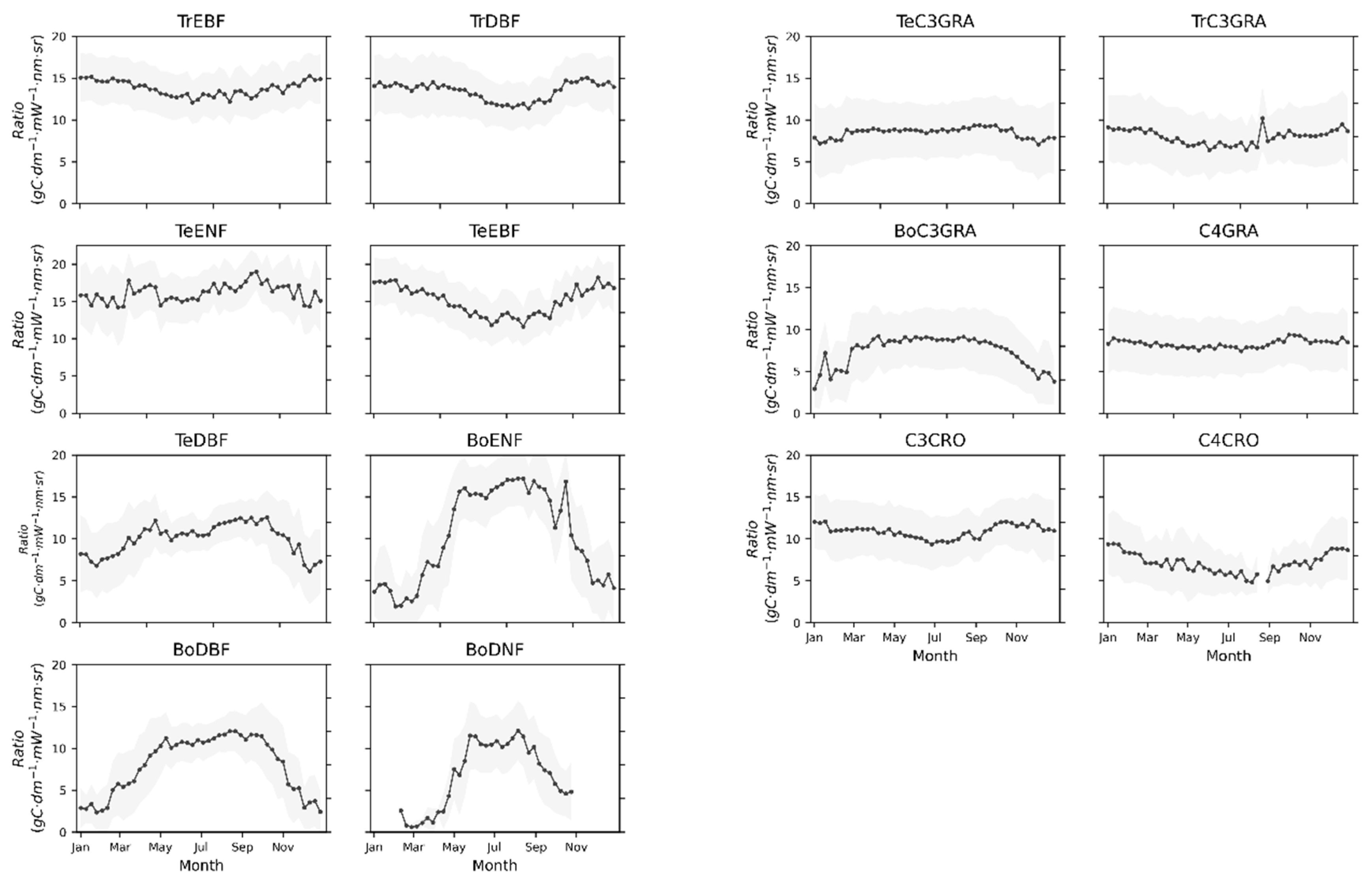
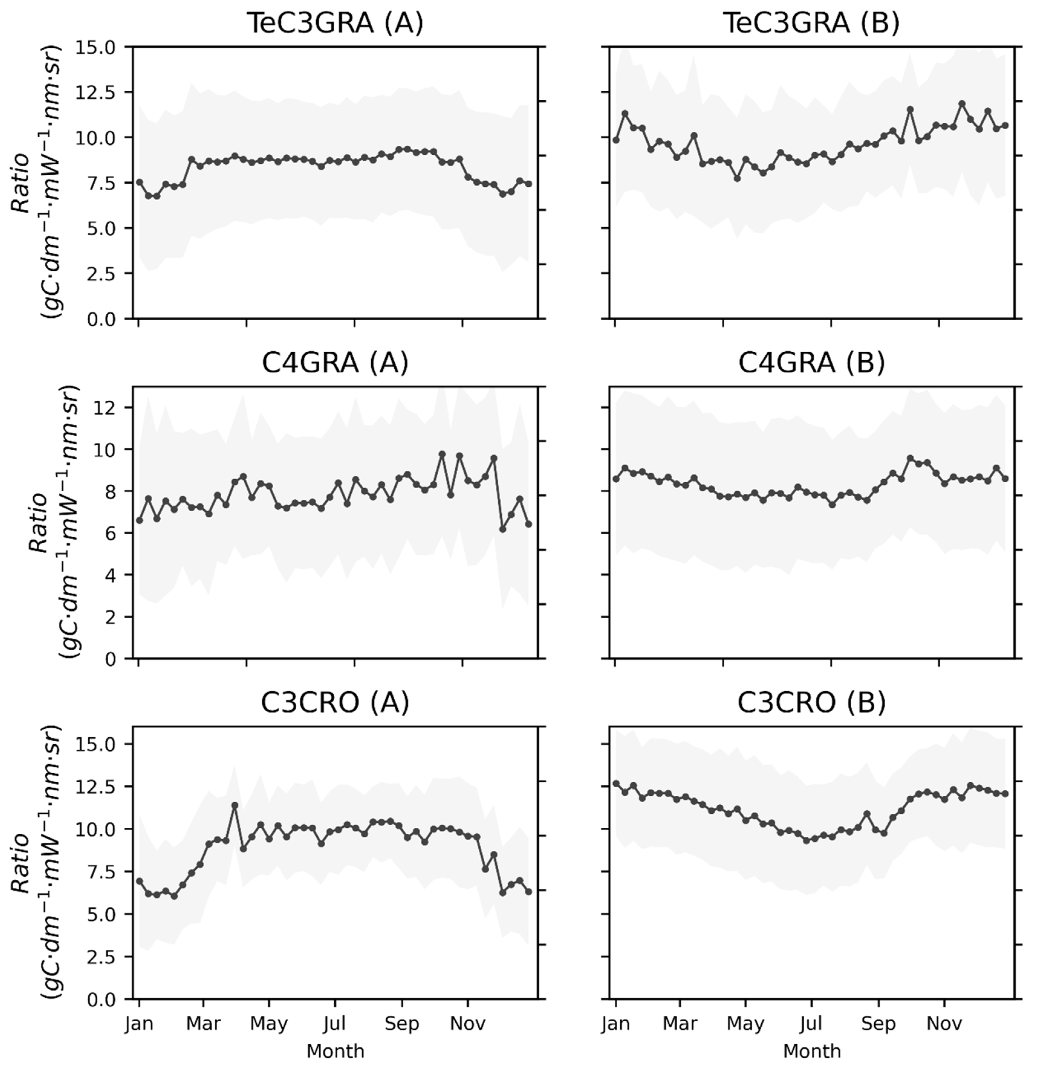
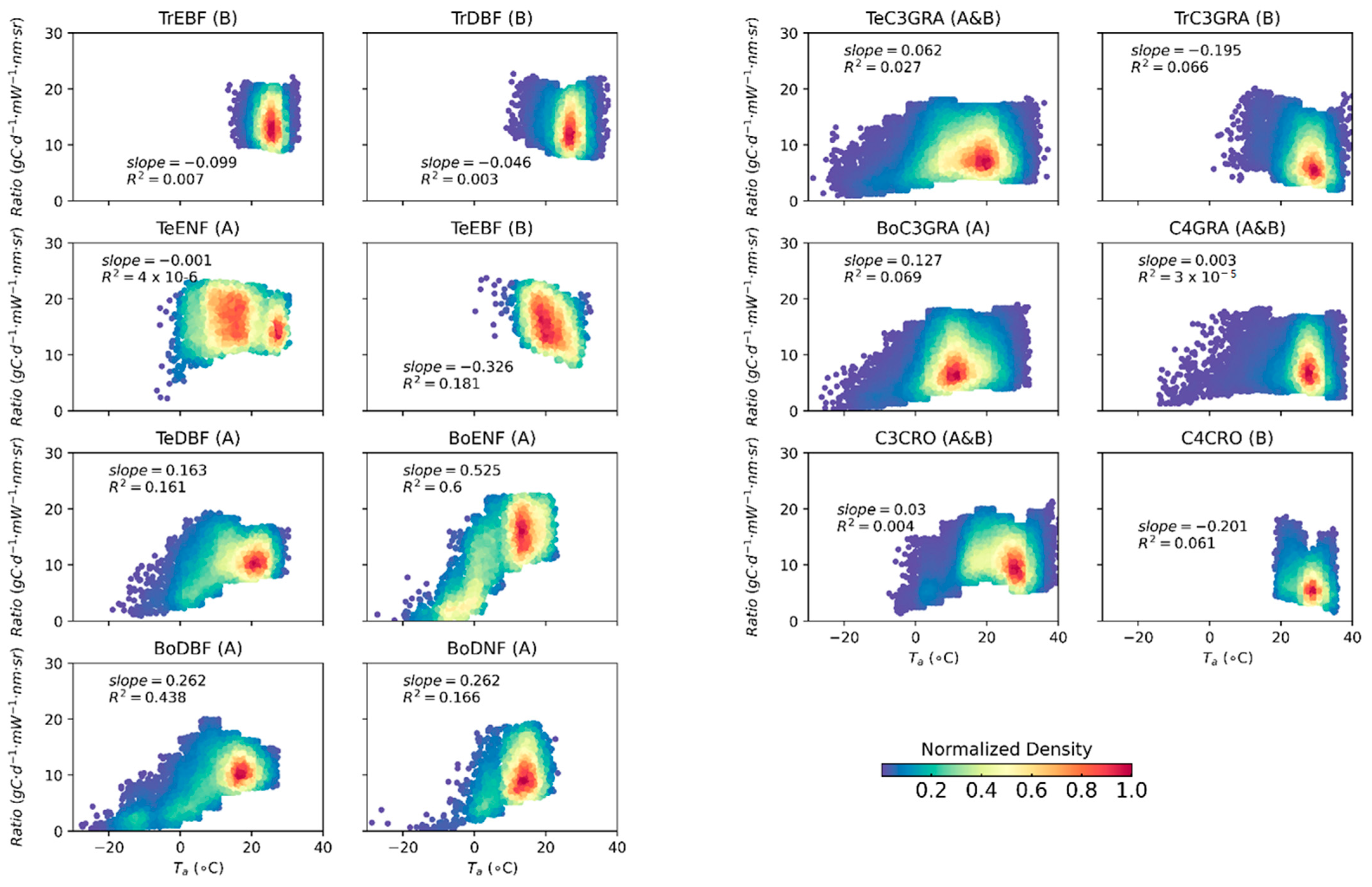
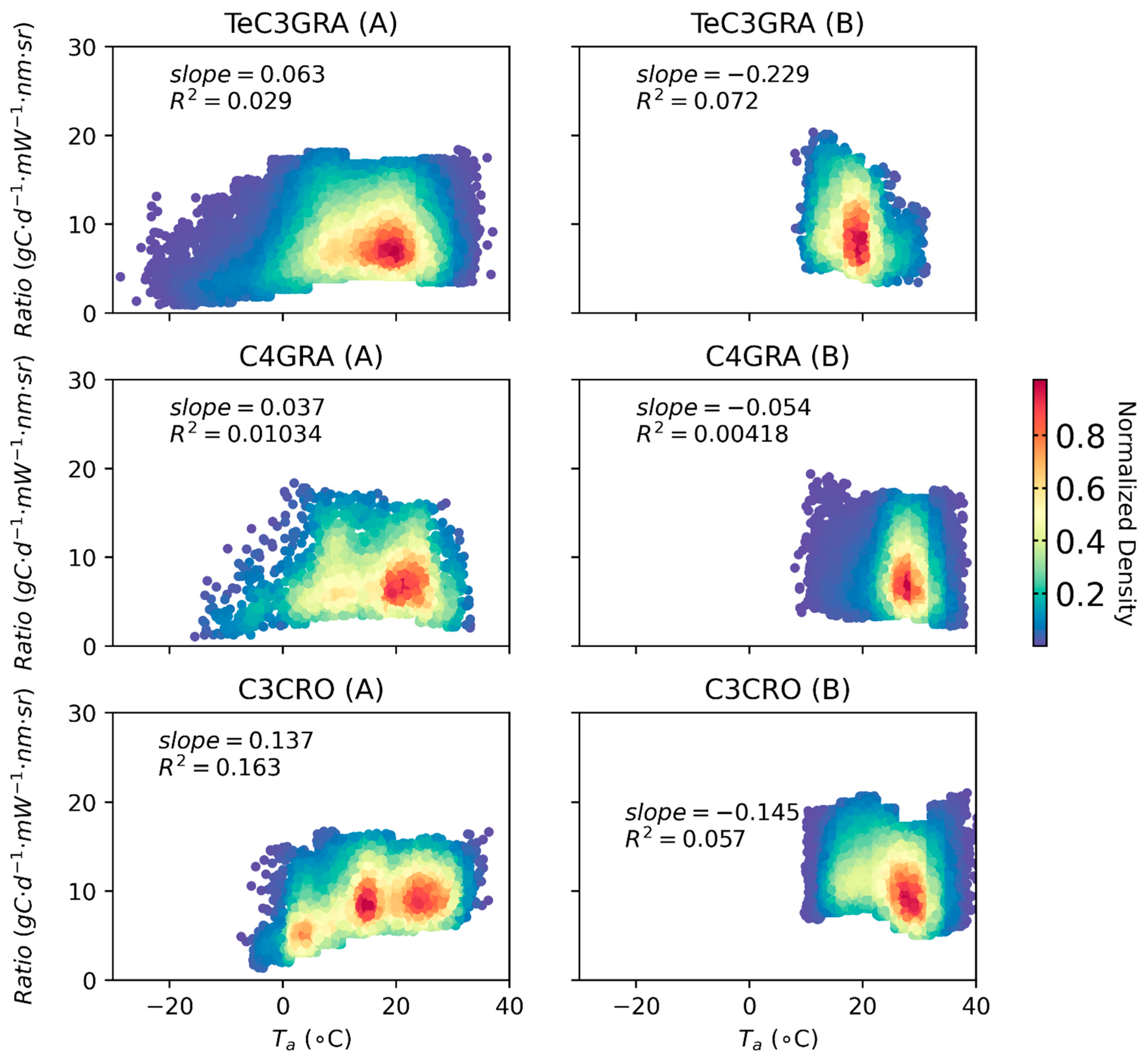
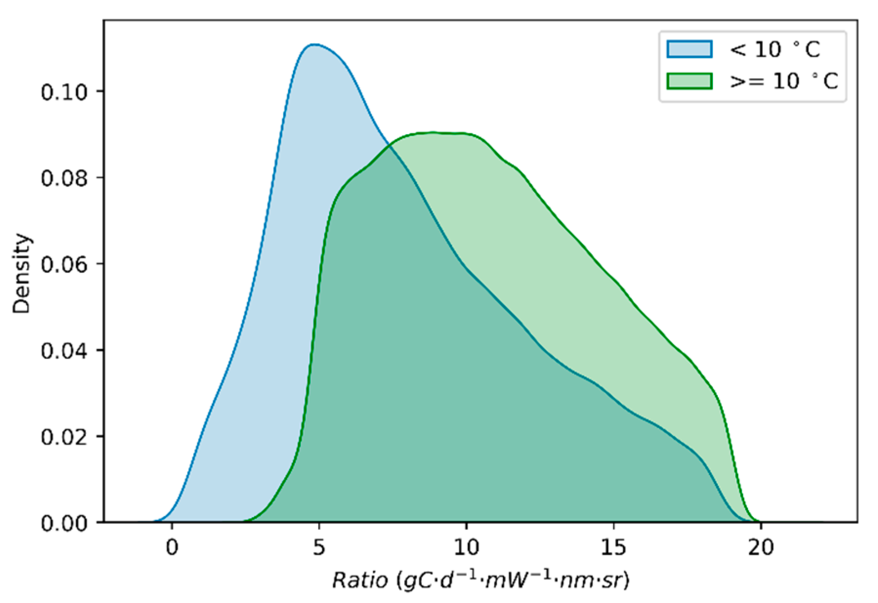
3.3. Effects of Low Temperature on the GPP/SIF Ratios for Different PFTs

From above results, we can see that temperature conditions affect the SIF–GPP relationship in some aspects. To further explore the different responses of SIF and GPP under low-temperature conditions, we investigated the relationship between the GPP/SIF ratio and temperature for different PFTs using both the satellite and tower-based data.

3.3.1. Global Satellite Dataset

As can be seen from Figure 9, we found that the seasonal pattern in the GPP/SIF ratio differed among PFTs. For tropical regions, TrEBF, TrDBF, and TrC3GRA generally exhibited a slightly “bowl-shaped” seasonal pattern for the GPP/SIF ratio. For temperate regions, TeEBF similarly presented a “bowl-shaped” seasonal variation in the GPP/SIF ratio, while the seasonal patterns of TeENF and TeDBF exhibited a slight “hump-shape”. For Boreal regions, BoENF, BoDBF, BoDNF, and BoC3GRA generally showed a clear “hump-shaped” seasonal pattern for the GPP/SIF ratio. In addition, the seasonal pattern of the GPP/SIF ratio for C4GRA, C3CRO, and C4CRO generally presented a “bowl-shape”. By reducing the effects of the canopy structure, the ratio of GPP to the total SIF (calculated as SIF divided by the escape probability; see the Supplementary Materials) also showed a “hump-shaped” pattern for many PFTs, while the “bowl-shaped” seasonal pattern was largely corrected, except for C4CRO (Figure S1).
Groups A of TeC3GRA, C4GRA, and C3GRA generally experienced more low-temperature stress than group B. From Figure 10, we can see that group A of TeC3GRA, C4GRA, and C3GRO generally showed a clear “’hump-shaped” seasonal pattern for the GPP/SIF ratio, whereas the corresponding B groups generally exhibited a slightly “bowl-shaped” seasonal pattern for the GPP/SIF ratio. It should be noted that the seasonal variations in the GPP/SIF ratio were affected by growth temperature conditions. For C3CRO, although all samples together exhibited a “bowl-shaped” seasonal pattern for the GPP/SIF ratio, group A separately exhibited a “hump-shaped” seasonal pattern. By reducing the effects of the canopy structure (Figure S2), a similar “hump-shape” can be observed in group A. Therefore, there were noticeable differences in the seasonal patterns of the GPP/SIF ratio between the selected samples that experienced low-temperature stress and those that grew under relatively warm conditions.
The influence of temperature conditions on the SIF–GPP relationship was further investigated using a linear regression and correlation analysis method. From Figure 11, we can see that the relationship between the GPP/SIF ratio and temperature differed among PFTs; however, the GPP/SIF ratio generally decreased under low-temperature conditions for some of those PFTs which experienced low-temperature stress. The GPP/SIF ratio generally exhibited a positive correlation with temperature in group A among the PFTs, while the GPP/SIF ratio in group B had no significant relationship with temperature (Figure 11; Table 3).
By separately controlling PAR and VPD, the partial correlation coefficients of the GPP/SIF ratio with temperature also demonstrated that the GPP/SIF ratio varied with temperature (Table 3). The GPP/SIF ratio in group A was found to be strongly positively correlated with temperature in the boreal region, where low-temperature stress conditions were more likely.
To better understand the differences between SIF and GPP in response to temperature, we further analyzed the correlation between the GPP/SIF ratio with temperature in groups A and B of TeC3GRA, C4GRA, and C3CRO, which had samples in both groups. From Figure 12, we can see that the slopes between the GPP/SIF ratio and temperature in group A were positive, while those in group B were negative. The distribution of the GPP/SIF ratio for the data when the temperature was above 10 °C differed from that obtained when temperature was below 10 °C (Figure 13). Therefore, the satellite data indicated that the GPP/SIF ratio was largely influenced by temperature conditions for different PFTs, and generally decreased in response to low-temperature conditions.

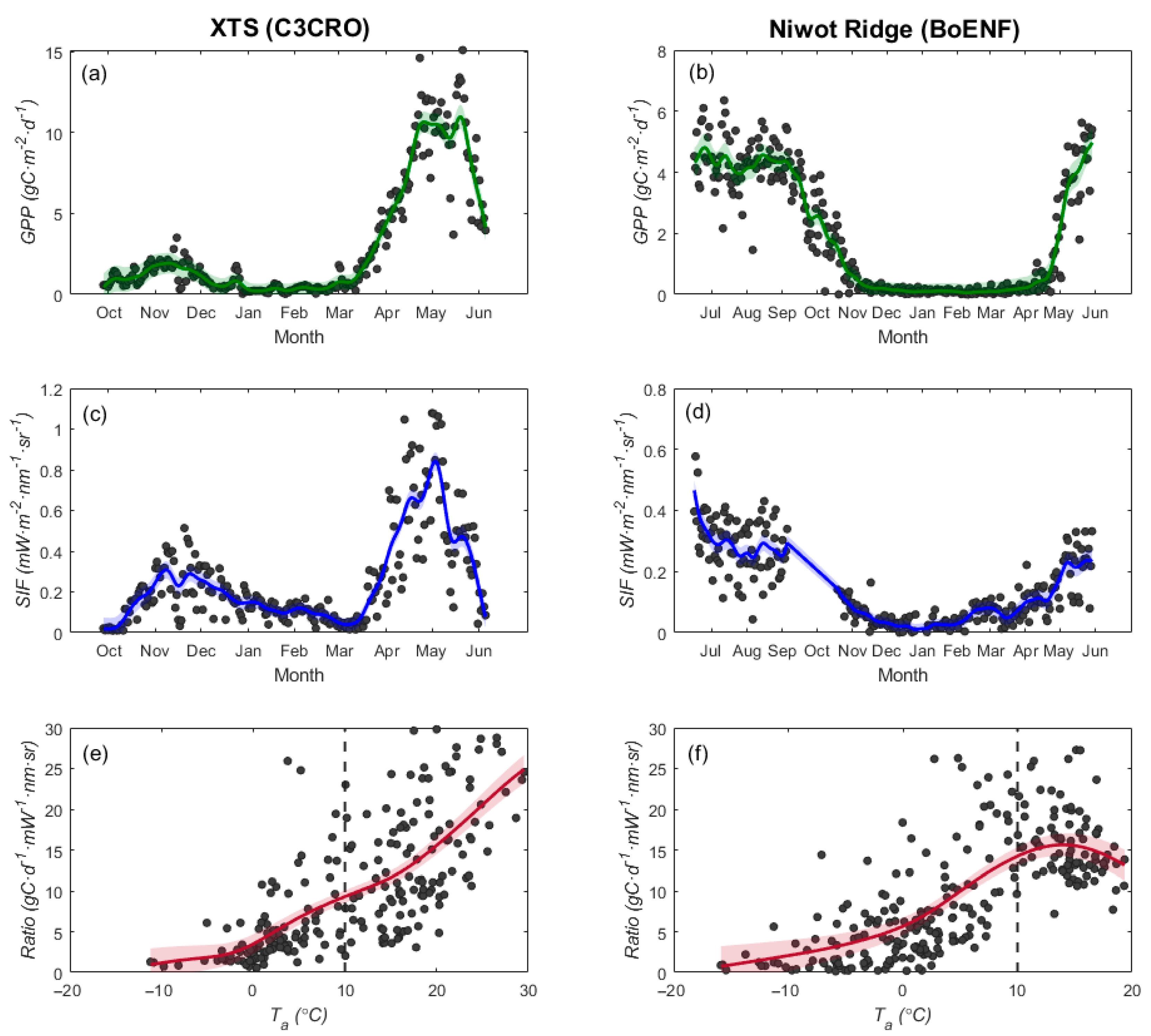
3.3.2. Tower-Based Dataset

Considering the tower-based observations, we can see that SIF tracked the GPP well during the over-wintering period for both the XTS (Figure 14a,c) and Niwot Ridge sites (Figure 14b,d). The GPP/SIF ratio in winter wheat (C3CRO) increased with temperature (Figure 14e); however, the GPP/SIF ratio in BoENF only increased with temperature when the temperature was below 10 °C. When the temperature was above 10 °C, the GPP/SIF ratio in BoENF decreased with temperature (Figure 14f). Therefore, the response of the GPP/SIF ratio to high temperatures might differ for different PFTs, which was different from the satellite results. This result needs to be further examined and verified. Nevertheless, the GPP/SIF ratio decreased under low-temperature conditions (below 10 °C) for both C3CRO and BoENF, consistent with the satellite results. The lower seasonal changes in the canopy structure and chlorophyll content in BoENF provide reliable evidence that the GPP/SIF ratio is associated with the changes in physiological factors influenced by a low temperature. The results also demonstrate that low temperatures affect the SIF–GPP relationships and highlight the importance of incorporating the effects of temperature into SIF-based GPP estimation.

4. Discussion

4.1. Why Does the GPP/SIF Ratio Decrease at Low Temperatures

Using satellite and tower-based data, we observed strong seasonal patterns in the GPP/SIF ratio and obvious differences in the GPP/SIF ratio for different PFTs. Although the SIF had a consistently seasonal pattern with GPP across different vegetation types, we found that there were noticeable differences in the seasonal patterns of the GPP/SIF ratios between the selected samples that experienced low-temperature stress (below 10 °C) and those that grew under relatively warm conditions (above 10 °C) (Figure 9 and Figure 10). The GPP/SIF ratio was generally positively related to temperatures below 10 °C, but did not consistently respond to temperatures above 10 °C (Figure 8, Table 2). For regions where low-temperature conditions do not occur (e.g., tropical regions), temperature may not be a factor limiting the GPP/SIF ratio (Figure 5 and Figure S1; [41,77]). Due to the selected samples in group A generally experiencing low-growth-temperature conditions (e.g., boreal ecosystems), with decreasing temperature, the GPP decreased faster than the SIF, and, hence, the GPP/SIF ratio declined again (Figure 9 and Figure S1; [42]). In addition, the tower-based measurements indicated that the response of the GPP/SIF ratio to high temperatures differed with different PFTs, which is inconsistent with the results obtained based on satellite data (Figure 11, Figure 12 and Figure 14e,f). However, the GPP/SIF ratio decreased at low temperatures (below 10 °C) for both C3CRO and BoENF in the results based on both satellite and tower-based observations. Small seasonal changes in canopy structure and chlorophyll content in BoENF also provide reliable evidence that the GPP/SIF ratio is related to changes in physiological factors affected by low temperatures. The GPP/SIF ratio generally had a low value at low temperatures, suggesting that the SIF–GPP relationship should be not assumed to be constant across PFTs and climates [1,57,78].
The reason why the GPP/SIF ratio decreases under low-temperature conditions may be attributed to the physiological differences between SIF and GPP in response to low temperature [21,79]. As SIF is closely related to light reactions, the differences between light and carbon reactions in response to environmental pressure may affect the SIF–GPP relationships [27,35,36]. Low temperatures impose thermodynamic constraints, slowing the enzymes related to the activities of the Calvin cycle. The decrease in photosynthetic enzyme activity with low temperature might explain the faster decrease in GPP than SIF, thus decreasing the GPP/SIF ratio [34]. In addition, the potential change of distribution in the absorbed energy among PQ, NPQ, and SIF may be another factor affecting the SIF–GPP relationship under low-temperature conditions [5]. Some studies have reported that the proportion of energy allocated to each energy-dissipated pathway is not constant under different environmental stresses [33]. Under low-temperature conditions, the light-harvesting complex (LHC) cannot completely utilize the absorbed light for CO2 fixation [49]. NPQ is an important photoprotective mechanism that plays a role in protecting photosystem II (PSII) from damage under low-temperature conditions [16,46]. Under NPQ changes, the dynamic range of PSII yields is much larger than that of the SIF yields, whereas sustained NPQ and deactivation of photosystems under low-temperature conditions may result in a reduction in SIF yields [9]. As SIF is mainly emitted from the chlorophyll molecules of PSII, a decrease in PSII productivity due to environmental stresses causes a chain of different protection mechanisms, which eventually decreases SIF [47,80,81,82]. Therefore, the potential physiological differences between SIF and GPP may explain why the GPP/SIF ratio decreased under low-temperature conditions.

4.2. Uncertainties and Limitations

In our study, we found that the GPP/SIF ratio differed for 14 vegetated PFTs using the TROPOMI SIF product and FLUXCOM GPP data. The GPP/SIF ratio for forest types was generally higher than that of grass and crop types, which is not consistent with previous research [58]. Li et al. [58] reported that there was a generally consistent slope of the SIF-GPP relationship among biomes using the OCO-2 SIF and flux tower GPP data. The reason why our results are not consistent with previous research may be as follows: (1) the different datasets used in research; (2) different biome types, as we used a vegetation map produced from CCI LC, LUH2 and a C3/C4 vegetation map, while Li et al. [58] used the MODIS Land Cover Type product (MCD12Q1) based on the University of Maryland (UMD) classification scheme; and (3) different linear fitting methods, as we used a linear regression with no intercept, while Li et al. [58] used a linear regression with an intercept. Theoretically, SIF is related to GPP through the coordinate origin. In addition, we found that the slope between GPP and SIF for C4CRO was lower than that for C3CRO, which is not consistent with the results of Li et al. [58]. In our study, the selected samples of C4CRO were mainly distributed at tropical regions (Figure 3) and could experience temperature and water stress. SIF is mainly driven by APAR and is also influenced by environmental stress (temperature and water stress), which determines photosynthetic light use efficiency (LUE). Therefore, both SIF and GPP for selected C4CRO samples had a lower value than that for selected C3CRO (Figure 3). Some studies have reported that the slope between GPP and SIF for C4CRO was generally higher than that for C3CRO [7,58]. However, the potential influences of environmental conditions and the distributions of different PFTs are ignored. In addition, less C4CRO samples were used, which may also have resulted in some uncertainties in our study.
The potential physiological changes caused by low-temperature conditions may result in the decrease in the GPP/SIF ratio in response to low temperatures. Group A of each PFT generally experienced low-temperature stress (below 10 °C), whereas group B of each PFT generally experienced relatively optimal temperature conditions (above 10 °C). In this study, we demonstrated that the seasonal patterns of the GPP/SIF ratio in group A of each PFT generally differed from those associated with group B, indicating that different temperatures affect the SIF–GPP relationship differently (Figure 12), especially under low-temperature conditions (Figure 13). The GPP/SIF ratio for group A generally exhibited a “hump-shaped” seasonal pattern, and that for group B showed a slightly “bowl-shaped” seasonal pattern. The above results are different from previous research that did not consider the effect of temperature conditions [34,58]. There were multiple sources of uncertainty in the seasonal variations in the GPP/SIF ratio [34].
The complex interactions of environmental factors (e.g., light intensity, temperature, and available water) on the photosynthetic activities play a role in changing the GPP/SIF ratio. Increasing light intensity led to a decline in the GPP/SIF ratio [3,21,38]. As the photosynthetic efficiency presents a non-linear decrease and the chlorophyll fluorescence quantum efficiency is not sensitive to increasing light intensity, the GPP exhibits a saturation effect under high light levels, while the SIF tends to continuously increase [37,83]. Decoupling of the GPP flux and SIF signals under water stress conditions may also alter the GPP/SIF ratio [41]. The rapid response of the stomatal conductance to water stress may explain the decline in the GPP/SIF ratio under water stress conditions [30,42]. Some studies have explored the performance of early water stress detection using leaf-level measurements of chlorophyll fluorescence and found that chlorophyll fluorescence decreased for plants with water stress relative to well-watered plants, while the filled watering experiment stated that chlorophyll fluorescence levels of maize under water stress were similar to those of well-watered maize [84]. Kimm et al. [45] also reported that the field-scale SIF yield (ФF) data showed water deficit stress from the comparison between irrigated and rain-fed corn field at three different spatial scales, and ФF was positively correlated with canopy-scale stomatal conductance, a reliable indicator of plant physiological condition. Chen et al. [42] found that decoupling of GPP and SIF under water stress conditions may also alter the GPP/SIF ratio, and the rapid response of the stomatal conductance to water stress may explain the decline in the GPP/SIF ratio under water stress conditions. Under optimal temperature conditions, the GPP/SIF ratio may be dominated by other environmental variables or changes in canopy structure, whereas under a wide temperature range including low-temperature conditions, the GPP/SIF ratio may be largely influenced by low temperatures [34]. In this study, we found that the GPP/SIF ratio was positively correlated with temperature for group A, indicating that the GPP-SIF relationship is affected by a wide temperature range, including low temperatures. In addition, the potential of using SIF to detect forest stresses, especially the defoliation of the plant by primary insects or foliar infection by pathogens, is of great interest [85]. However, current studies generally ignore the crown heterogeneity caused by pests. The impact of structural properties of damaged foliage on canopy SIF, as well as the response of the GPP/SIF ratio to pest-damage, has not been well-explored.
Despite the potential effects of environmental pressures, the GPP/SIF ratio is also affected by the leaf age, leaf phenology, and leaf chlorophyll content during the growing period [30]. Some studies have reported that the seasonal peak timing of APAR played a dominated role in the seasonal peak timing of far-red SIF, whereas the seasonal peak timing of chlorophyll content contributed more to the seasonal peak timing of GPP [30,46]. The seasonal difference between far-red SIF and GPP is, thus, possibly more strongly determined by the seasonal changes in the APAR and canopy chlorophyll content [30]. Therefore, the seasonal GPP/SIF variation may also be affected by the seasonal variations in vegetation function traits.
Canopy structure can also play a role in forming the seasonal pattern of the GPP/SIF ratio [18,25,27]. The seasonal variations in canopy structure can lead to the changes in the escape probability (fesc), which further affects the observed SIF. The fesc is generally lower when the canopy is denser during the growing season. Some studies have reported that a denser canopy structure can also lead to a higher GPP/SIF ratio [86]. Remote-observed SIF is only part of the total emitted SIF by leaves, which can experience a large number of scattering and reabsorption effects [87]. To reduce the effects of the canopy structure, we explored the seasonal variations in the ratio of GPP to the total SIF (defined as GPP/tSIF, Figures S1–S3). A similar “hump-shaped” seasonal pattern of GPP/tSIF was found in many PFTs, while the “bowl-shaped” seasonal pattern of GPP/SIF for some PFTs was largely corrected. Although this indicates that the canopy structure affects the seasonal variation in GPP/SIF, a decline in GPP/tSIF was also found under low-temperature conditions (Figures S1–S3). By reducing the potential contribution of the canopy structure to the change in GPP/SIF, we can better explore the seasonal pattern in GPP/SIF under changeable climates. Therefore, this study provided a reliable evaluation of the seasonal variation in GPP/SIF by separating the data into two groups based on different growth temperature conditions.
In addition, improvement of the remote estimation of GPP is the ultimate motivation for studying the SIF–GPP relationship [34,88]. Large-scale GPP estimation relies on fine spatio-temporal satellite SIF products [89]. In this study, we used the aggregated eight-day TROPOMI SIF to obtain more data at the global scale. Future SIF products could provide daily and sub-daily observations, which would be more valuable for studying the SIF–GPP relationship under changeable environmental conditions. In addition, some studies have reported that an increased cloud fraction threshold can result in a decrease in estimated SIF [90]. Therefore, the availabilities would impact the number of selected samples for each PFT used to analyze the different responses of SIF and GPP to low temperatures.
Overall, our analyses revealed obvious differences in the seasonal patterns of SIF and GPP under different growth temperature conditions, where the GPP/SIF ratio decreased under low-temperature conditions. The decrease in GPP/SIF with low temperatures highlighted the importance of considering this behavior when estimating GPP from satellite SIF observations [91]. Future studies should conduct more field experiments to explore the potential physiological and structural factors affecting the seasonal patterns of SIF and GPP. Although the mechanisms underlying the seasonal GPP/SIF patterns under environmental pressure require further investigation, the results obtained in this study regarding the effects of low temperatures on the SIF–GPP relationship can help to improve our understanding of the SIF-GPP relationship.

5. Conclusions

We investigated the seasonal variations in the ratio of the GPP to the far-red SIF across various PFTs using both satellite and tower-based data. The GPP/SIF ratio for forest types was generally higher than that of grass and crop types. There were also noticeable differences in the seasonal pattern of the GPP/SIF ratio between the selected samples experiencing low-temperature stress (below 10 °C) and those growing in relatively warm conditions (above 10 °C throughout the year). For the data with a wide temperature range, including low-temperature conditions, we observed a positive relationship between the GPP/SIF ratio and temperature; however, the relationship did not consistently respond to temperature when considering data for temperatures above 10 °C throughout the year. Overall, the results demonstrate that the relationship between the GPP/SIF ratio and temperature was not constant among PFTs, as the GPP/SIF ratio decreased under low-temperature conditions for some PFTs experiencing low-temperature stress. Therefore, our findings highlight the importance of incorporating the temperature into SIF-based GPP estimation.

Supplementary Materials

The following supporting information can be downloaded at: https://www.mdpi.com/article/10.3390/rs14153716/s1.

Author Contributions

Conceptualization, X.L.; Formal analysis, L.L.; Methodology, J.C.; Writing—original draft, J.C.; Writing—review and editing, X.L., Y.M. and L.L. All authors have read and agreed to the published version of the manuscript.

Funding

This research was funded by the National Natural Science Foundation of China, grant number 41825002, 42071310.

Data Availability Statement

TROPOMI SIF products are available at https://s5p-troposif.noveltis.fr/data-access. The ERA5-Land reanalysis dataset is available at https://cds.climate.copernicus.eu/. FLUXCOM GPP products with customized ensemble estimates are available on request to Martin Jung (mjung@bgc-jena.mpg.de). The XTS site data are available from the authors upon request. Niwot Ridge site data are available at a data repository (https://data.caltech.edu/records/1231) hosted at the California Institute of Technology.

Acknowledgments

This work was supported by the National Natural Science Foundation of China (grant 41825002, 42071310). We also thank the California Institute of Technology for providing the data for the Niwot Ridge site. We are grateful to G.Y.’s team for supplying the experiment equipment and flux data for the XTS site. J.C., X.L. and L.L. contributed to the experiment design and research method. J.C. and Y.M. performed analysis and writing of the manuscript.

Conflicts of Interest

The authors declare no conflict of interest.

References

  1. Beer, C.; Reichstein, M.; Tomelleri, E.; Ciais, P.; Jung, M.; Carvalhais, N.; Rödenbeck, C.; Arain, M.A.; Baldocchi, D.; Bonan, G.B. Terrestrial gross carbon dioxide uptake: Global distribution and covariation with climate. Science 2010, 329, 834–838. [Google Scholar] [CrossRef] [PubMed] [Green Version]
  2. Verma, M.; Schimel, D.; Evans, B.; Frankenberg, C.; Beringer, J.; Drewry, D.T.; Magney, T.; Marang, I.; Hutley, L.; Moore, C. Effect of environmental conditions on the relationship between solar-induced fluorescence and gross primary productivity at an OzFlux grassland site. J. Geophys. Res. Biogeosci. 2017, 122, 716–733. [Google Scholar] [CrossRef] [Green Version]
  3. Porcar-Castell, A.; Tyystjärvi, E.; Atherton, J.; Van der Tol, C.; Flexas, J.; Pfündel, E.E.; Moreno, J.; Frankenberg, C.; Berry, J.A. Linking chlorophyll a fluorescence to photosynthesis for remote sensing applications: Mechanisms and challenges. J. Exp. Bot. 2014, 65, 4065–4095. [Google Scholar] [CrossRef] [PubMed]
  4. Frankenberg, C.; Fisher, J.B.; Worden, J.; Badgley, G.; Saatchi, S.S.; Lee, J.E.; Toon, G.C.; Butz, A.; Jung, M.; Kuze, A. New global observations of the terrestrial carbon cycle from GOSAT: Patterns of plant fluorescence with gross primary productivity. Geophys. Res. Lett. 2011, 38. [Google Scholar] [CrossRef] [Green Version]
  5. Berry, J.A.; Frankenberg, C.; Wennberg, P. New Methods for Measurements of Photosynthesis from Space. 2013. Available online: https://www.researchgate.net/publication/331141053_New_Methods_for_Measurements_of_Photosynthesis_from_Space (accessed on 1 December 2021). [CrossRef]
  6. Guanter, L.; Aben, I.; Tol, P.; Krijger, J.; Hollstein, A.; Köhler, P.; Damm, A.; Joiner, J.; Frankenberg, C.; Landgraf, J. Potential of the TROPOspheric Monitoring Instrument (TROPOMI) onboard the Sentinel-5 Precursor for the monitoring of terrestrial chlorophyll fluorescence. Atmos. Meas. Tech. 2015, 8, 1337–1352. [Google Scholar] [CrossRef] [Green Version]
  7. Liu, L.; Guan, L.; Liu, X. Directly estimating diurnal changes in GPP for C3 and C4 crops using far-red sun-induced chlorophyll fluorescence. Agric. For. Meteorol. 2017, 232, 1–9. [Google Scholar] [CrossRef]
  8. Bacour, C.; Maignan, F.; MacBean, N.; Porcar-Castell, A.; Flexas, J.; Frankenberg, C.; Peylin, P.; Chevallier, F.; Vuichard, N.; Bastrikov, V. Improving estimates of gross primary productivity by assimilating solar-induced fluorescence satellite retrievals in a terrestrial biosphere model using a process-based SIF model. J. Geophys. Res. Biogeosci. 2019, 124, 3281–3306. [Google Scholar] [CrossRef]
  9. Magney, T.S.; Bowling, D.R.; Logan, B.A.; Grossmann, K.; Stutz, J.; Blanken, P.D.; Burns, S.P.; Cheng, R.; Garcia, M.A.; Köhler, P. Mechanistic evidence for tracking the seasonality of photosynthesis with solar-induced fluorescence. Proc. Natl. Acad. Sci. USA 2019, 116, 11640–11645. [Google Scholar] [CrossRef] [Green Version]
  10. Monteith, J. Solar radiation and productivity in tropical ecosystems. J. Appl. Ecol. 1972, 9, 747–766. [Google Scholar] [CrossRef] [Green Version]
  11. Berry, J.; Wolf, A.; Campbell, J.E.; Baker, I.; Blake, N.; Blake, D.; Denning, A.S.; Kawa, S.R.; Montzka, S.A.; Seibt, U. A coupled model of the global cycles of carbonyl sulfide and CO2: A possible new window on the carbon cycle. J. Geophys. Res. Biogeosci. 2013, 118, 842–852. [Google Scholar] [CrossRef] [Green Version]
  12. Guanter, L.; Frankenberg, C.; Dudhia, A.; Lewis, P.E.; Gómez-Dans, J.; Kuze, A.; Suto, H.; Grainger, R.G. Retrieval and global assessment of terrestrial chlorophyll fluorescence from GOSAT space measurements. Remote Sens. Environ. 2012, 121, 236–251. [Google Scholar] [CrossRef]
  13. Zhang, Y.; Guanter, L.; Berry, J.A.; van der Tol, C.; Yang, X.; Tang, J.; Zhang, F. Model-based analysis of the relationship between sun-induced chlorophyll fluorescence and gross primary production for remote sensing applications. Remote Sens. Environ. 2016, 187, 145–155. [Google Scholar] [CrossRef] [Green Version]
  14. Sun, Y.; Frankenberg, C.; Wood, J.D.; Schimel, D.; Jung, M.; Guanter, L.; Drewry, D.; Verma, M.; Porcar-Castell, A.; Griffis, T.J. OCO-2 advances photosynthesis observation from space via solar-induced chlorophyll fluorescence. Science 2017, 358, eaam5747. [Google Scholar] [CrossRef] [PubMed] [Green Version]
  15. Yang, K.; Ryu, Y.; Dechant, B.; Berry, J.A.; Hwang, Y.; Jiang, C.; Kang, M.; Kim, J.; Kimm, H.; Kornfeld, A. Sun-induced chlorophyll fluorescence is more strongly related to absorbed light than to photosynthesis at half-hourly resolution in a rice paddy. Remote Sens. Environ. 2018, 216, 658–673. [Google Scholar] [CrossRef]
  16. Wang, N.; Clevers, J.G.; Wieneke, S.; Bartholomeus, H.; Kooistra, L. Potential of UAV-based sun-induced chlorophyll fluorescence to detect water stress in sugar beet. Agric. For. Meteorol. 2022, 323, 109033. [Google Scholar] [CrossRef]
  17. Baker, N.R. Chlorophyll fluorescence: A probe of photosynthesis in vivo. Annu. Rev. Plant Biol. 2008, 59, 89. [Google Scholar] [CrossRef] [PubMed] [Green Version]
  18. Zeng, Y.; Badgley, G.; Dechant, B.; Ryu, Y.; Chen, M.; Berry, J.A. A practical approach for estimating the escape ratio of near-infrared solar-induced chlorophyll fluorescence. Remote Sens. Environ. 2019, 232, 111209. [Google Scholar] [CrossRef] [Green Version]
  19. Doughty, R.; Xiao, X.; Köhler, P.; Frankenberg, C.; Qin, Y.; Wu, X.; Ma, S.; Moore, B., III. Global-Scale Consistency of Spaceborne Vegetation Indices, Chlorophyll Fluorescence, and Photosynthesis. J. Geophys. Res. Biogeosci. 2021, 126, e2020JG006136. [Google Scholar] [CrossRef]
  20. Adams, W.W.; Demmig-Adams, B. Chlorophyll fluorescence as a tool to monitor plant response to the environment. In Chlorophyll A Fluorescence; Springer: Berlin/Heidelberg, Germany, 2004; pp. 583–604. [Google Scholar]
  21. Gu, L.; Han, J.; Wood, J.D.; Chang, C.Y.Y.; Sun, Y. Sun-induced Chl fluorescence and its importance for biophysical modeling of photosynthesis based on light reactions. New Phytol. 2019, 223, 1179–1191. [Google Scholar] [CrossRef] [Green Version]
  22. Wood, J.D.; Griffis, T.J.; Baker, J.M.; Frankenberg, C.; Verma, M.; Yuen, K. Multiscale analyses of solar-induced florescence and gross primary production. Geophys. Res. Lett. 2017, 44, 533–541. [Google Scholar] [CrossRef]
  23. Liu, X.; Guanter, L.; Liu, L.; Damm, A.; Malenovský, Z.; Rascher, U.; Peng, D.; Du, S.; Gastellu-Etchegorry, J.-P. Downscaling of solar-induced chlorophyll fluorescence from canopy level to photosystem level using a random forest model. Remote Sens. Environ. 2019, 231, 110772. [Google Scholar] [CrossRef]
  24. Romero, J.M.; Cordon, G.B.; Lagorio, M.G. Re-absorption and scattering of chlorophyll fluorescence in canopies: A revised approach. Remote Sens. Environ. 2020, 246, 111860. [Google Scholar] [CrossRef]
  25. Zhang, Z.; Zhang, Y.; Chen, J.M.; Ju, W.; Migliavacca, M.; El-Madany, T.S. Sensitivity of estimated total canopy SIF emission to remotely sensed LAI and BRDF products. J. Remote Sens. 2021, 2021, 9795837. [Google Scholar] [CrossRef]
  26. Migliavacca, M.; Perez-Priego, O.; Rossini, M.; El-Madany, T.S.; Moreno, G.; Van der Tol, C.; Rascher, U.; Berninger, A.; Bessenbacher, V.; Burkart, A. Plant functional traits and canopy structure control the relationship between photosynthetic CO2 uptake and far-red sun-induced fluorescence in a Mediterranean grassland under different nutrient availability. New Phytol. 2017, 214, 1078–1091. [Google Scholar] [CrossRef] [PubMed] [Green Version]
  27. Dechant, B.; Ryu, Y.; Badgley, G.; Zeng, Y.; Berry, J.A.; Zhang, Y.; Goulas, Y.; Li, Z.; Zhang, Q.; Kang, M. Canopy structure explains the relationship between photosynthesis and sun-induced chlorophyll fluorescence in crops. Remote Sens. Environ. 2020, 241, 111733. [Google Scholar] [CrossRef] [Green Version]
  28. Liu, X.; Liu, L.; Hu, J.; Guo, J.; Du, S. Improving the potential of red SIF for estimating GPP by downscaling from the canopy level to the photosystem level. Agric. For. Meteorol. 2020, 281, 107846. [Google Scholar] [CrossRef]
  29. Dechant, B.; Ryu, Y.; Badgley, G.; Köhler, P.; Rascher, U.; Migliavacca, M.; Zhang, Y.; Tagliabue, G.; Guan, K.; Rossini, M. NIRVP: A robust structural proxy for sun-induced chlorophyll fluorescence and photosynthesis across scales. Remote Sens. Environ. 2022, 268, 112763. [Google Scholar] [CrossRef]
  30. Wu, G.; Jiang, C.; Kimm, H.; Wang, S.; Bernacchi, C.; Moore, C.E.; Suyker, A.; Yang, X.; Magney, T.; Frankenberg, C. Difference in seasonal peak timing of soybean far-red SIF and GPP explained by canopy structure and chlorophyll content. Remote Sens. Environ. 2022, 279, 113104. [Google Scholar] [CrossRef]
  31. Paul-Limoges, E.; Damm, A.; Hueni, A.; Liebisch, F.; Eugster, W.; Schaepman, M.E.; Buchmann, N. Effect of environmental conditions on sun-induced fluorescence in a mixed forest and a cropland. Remote Sens. Environ. 2018, 219, 310–323. [Google Scholar] [CrossRef]
  32. Ač, A.; Malenovský, Z.; Olejníčková, J.; Gallé, A.; Rascher, U.; Mohammed, G. Meta-analysis assessing potential of steady-state chlorophyll fluorescence for remote sensing detection of plant water, temperature and nitrogen stress. Remote Sens. Environ. 2015, 168, 420–436. [Google Scholar] [CrossRef] [Green Version]
  33. Flexas, J.; Escalona, J.M.; Evain, S.; Gulías, J.; Moya, I.; Osmond, C.B.; Medrano, H. Steady-state chlorophyll fluorescence (Fs) measurements as a tool to follow variations of net CO2 assimilation and stomatal conductance during water-stress in C3 plants. Physiol. Plant. 2002, 114, 231–240. [Google Scholar] [CrossRef] [PubMed] [Green Version]
  34. Chen, A.; Mao, J.; Ricciuto, D.; Lu, D.; Xiao, J.; Li, X.; Thornton, P.E.; Knapp, A.K. Seasonal changes in GPP/SIF ratios and their climatic determinants across the Northern Hemisphere. Glob. Chang. Biol. 2021, 27, 5186–5197. [Google Scholar] [CrossRef]
  35. Farquhar, G.; Wong, S.; Evans, J.; Hubick, K. Photosynthesis and gas exchange. In Plants Under Stress; Cambridge University Press: Cambridge, UK, 1989; Volume 39, pp. 47–69. [Google Scholar] [CrossRef]
  36. Ögren, E.; Evans, J. Photosynthetic light-response curves. Planta 1993, 189, 182–190. [Google Scholar] [CrossRef]
  37. Chen, J.; Liu, X.; Du, S.; Ma, Y.; Liu, L. Integrating sif and clearness index to improve maize GPP estimation using continuous tower-based observations. Sensors 2020, 20, 2493. [Google Scholar] [CrossRef] [PubMed]
  38. Liu, X.; Liu, Z.; Liu, L.; Lu, X.; Chen, J.; Du, S.; Zou, C. Modelling the influence of incident radiation on the SIF-based GPP estimation for maize. Agric. For. Meteorol. 2021, 307, 108522. [Google Scholar] [CrossRef]
  39. Sun, Y.; Fu, R.; Dickinson, R.; Joiner, J.; Frankenberg, C.; Gu, L.; Xia, Y.; Fernando, N. Drought onset mechanisms revealed by satellite solar-induced chlorophyll fluorescence: Insights from two contrasting extreme events. J. Geophys. Res. Biogeosci. 2015, 120, 2427–2440. [Google Scholar] [CrossRef]
  40. Wang, X.; Qiu, B.; Li, W.; Zhang, Q. Impacts of drought and heatwave on the terrestrial ecosystem in China as revealed by satellite solar-induced chlorophyll fluorescence. Sci. Total Environ. 2019, 693, 133627. [Google Scholar] [CrossRef] [PubMed]
  41. Helm, L.T.; Shi, H.; Lerdau, M.T.; Yang, X. Solar-induced chlorophyll fluorescence and short-term photosynthetic response to drought. Ecol. Appl. 2020, 30, e02101. [Google Scholar] [CrossRef]
  42. Chen, J.; Liu, X.; Du, S.; Ma, Y.; Liu, L. Effects of Drought on the Relationship Between Photosynthesis and Chlorophyll Fluorescence for Maize. IEEE J. Sel. Top. Appl. Earth Obs. Remote Sens. 2021, 14, 11148–11161. [Google Scholar] [CrossRef]
  43. Zhuang, J.; Wang, Y.; Chi, Y.; Zhou, L.; Chen, J.; Zhou, W.; Song, J.; Zhao, N.; Ding, J. Drought stress strengthens the link between chlorophyll fluorescence parameters and photosynthetic traits. PeerJ 2020, 8, e10046. [Google Scholar] [CrossRef] [PubMed]
  44. Song, L.; Guanter, L.; Guan, K.; You, L.; Huete, A.; Ju, W.; Zhang, Y. Satellite sun-induced chlorophyll fluorescence detects early response of winter wheat to heat stress in the Indian Indo-Gangetic Plains. Glob. Chang. Biol. 2018, 24, 4023–4037. [Google Scholar] [CrossRef] [PubMed] [Green Version]
  45. Kimm, H.; Guan, K.; Burroughs, C.H.; Peng, B.; Ainsworth, E.A.; Bernacchi, C.J.; Moore, C.E.; Kumagai, E.; Yang, X.; Berry, J.A. Quantifying high-temperature stress on soybean canopy photosynthesis: The unique role of sun-induced chlorophyll fluorescence. Glob. Chang. Biol. 2021, 27, 2403–2415. [Google Scholar] [CrossRef] [PubMed]
  46. Kim, J.; Ryu, Y.; Dechant, B.; Lee, H.; Kim, H.S.; Kornfeld, A.; Berry, J.A. Solar-induced chlorophyll fluorescence is non-linearly related to canopy photosynthesis in a temperate evergreen needleleaf forest during the fall transition. Remote Sens. Environ. 2021, 258, 112362. [Google Scholar] [CrossRef]
  47. Fracheboud, Y.; Leipner, J. The application of chlorophyll fluorescence to study light, temperature, and drought stress. In Practical Applications of Chlorophyll Fluorescence in Plant Biology; Springer: Berlin/Heidelberg, Germany, 2003; pp. 125–150. [Google Scholar]
  48. Sippel, S.; Meinshausen, N.; Fischer, E.M.; Székely, E.; Knutti, R. Climate change now detectable from any single day of weather at global scale. Nat. Clim. Chang. 2020, 10, 35–41. [Google Scholar] [CrossRef]
  49. Li, Y.-N.; Li, Y.-T.; Ivanov, A.G.; Jiang, W.-L.; Che, X.-K.; Liang, Y.; Zhang, Z.-S.; Zhao, S.-J.; Gao, H.-Y. Defective photosynthetic adaptation mechanism in winter restricts the introduction of overwintering plant to high latitudes. bioRxiv 2019, 613117. [Google Scholar] [CrossRef]
  50. Fracheboud, Y.; Jompuk, C.; Ribaut, J.; Stamp, P.; Leipner, J. Genetic analysis of cold-tolerance of photosynthesis in maize. Plant Mol. Biol. 2004, 56, 241–253. [Google Scholar] [CrossRef]
  51. Pickering, M.; Cescatti, A.; Duveiller, G. Sun-Induced Fluorescence as a Proxy of Primary Productivity across Vegetation Types and Climates. Biogeosci. Discuss. 2022, 1–33. [Google Scholar] [CrossRef]
  52. Guanter, L.; Zhang, Y.; Jung, M.; Joiner, J.; Voigt, M.; Berry, J.A.; Frankenberg, C.; Huete, A.R.; Zarco-Tejada, P.; Lee, J.-E. Global and time-resolved monitoring of crop photosynthesis with chlorophyll fluorescence. Proc. Natl. Acad. Sci. USA 2014, 111, E1327–E1333. [Google Scholar] [CrossRef] [Green Version]
  53. Guanter, L.; Bacour, C.; Schneider, A.; Aben, I.; van Kempen, T.A.; Maignan, F.; Retscher, C.; Köhler, P.; Frankenberg, C.; Joiner, J. The TROPOSIF global sun-induced fluorescence dataset from the Sentinel-5P TROPOMI mission. Earth Syst. Sci. Data 2021, 13, 5423–5440. [Google Scholar] [CrossRef]
  54. Köhler, P.; Frankenberg, C.; Magney, T.S.; Guanter, L.; Joiner, J.; Landgraf, J. Global retrievals of solar-induced chlorophyll fluorescence with TROPOMI: First results and intersensor comparison to OCO-2. Geophys. Res. Lett. 2018, 45, 10456–10463. [Google Scholar] [CrossRef] [PubMed] [Green Version]
  55. Miao, G.; Guan, K.; Yang, X.; Bernacchi, C.J.; Berry, J.A.; DeLucia, E.H.; Wu, J.; Moore, C.E.; Meacham, K.; Cai, Y. Sun-induced chlorophyll fluorescence, photosynthesis, and light use efficiency of a soybean field from seasonally continuous measurements. J. Geophys. Res. Biogeosci. 2018, 123, 610–623. [Google Scholar] [CrossRef]
  56. Zhang, Y.; Zhang, Q.; Liu, L.; Zhang, Y.; Wang, S.; Ju, W.; Zhou, G.; Zhou, L.; Tang, J.; Zhu, X. ChinaSpec: A Network for Long-Term Ground-Based Measurements of Solar-Induced Fluorescence in China. J. Geophys. Res. Biogeosci. 2021, 126, e2020JG006042. [Google Scholar] [CrossRef]
  57. Liu, Z.; Zhao, F.; Liu, X.; Yu, Q.; Wang, Y.; Peng, X.; Cai, H.; Lu, X. Direct estimation of photosynthetic CO2 assimilation from solar-induced chlorophyll fluorescence (SIF). Remote Sens. Environ. 2022, 271, 112893. [Google Scholar] [CrossRef]
  58. Li, X.; Xiao, J.; He, B.; Altaf Arain, M.; Beringer, J.; Desai, A.R.; Emmel, C.; Hollinger, D.Y.; Krasnova, A.; Mammarella, I. Solar-induced chlorophyll fluorescence is strongly correlated with terrestrial photosynthesis for a wide variety of biomes: First global analysis based on OCO-2 and flux tower observations. Glob. Chang. Biol. 2018, 24, 3990–4008. [Google Scholar] [CrossRef] [PubMed]
  59. Frankenberg, C.; O’Dell, C.; Guanter, L.; McDuffie, J. Remote sensing of near-infrared chlorophyll fluorescence from space in scattering atmospheres: Implications for its retrieval and interferences with atmospheric CO2 retrievals. Atmos. Meas. Tech. 2012, 5, 2081–2094. [Google Scholar] [CrossRef] [Green Version]
  60. Wang, S.; Zhang, Y.; Ju, W.; Qiu, B.; Zhang, Z. Tracking the seasonal and inter-annual variations of global gross primary production during last four decades using satellite near-infrared reflectance data. Sci. Total Environ. 2021, 755, 142569. [Google Scholar] [CrossRef]
  61. Jung, M.; Koirala, S.; Weber, U.; Ichii, K.; Gans, F.; Camps-Valls, G.; Papale, D.; Schwalm, C.; Tramontana, G.; Reichstein, M. The FLUXCOM ensemble of global land-atmosphere energy fluxes. Sci. Data 2019, 6, 74. [Google Scholar] [CrossRef] [PubMed] [Green Version]
  62. Jung, M.; Schwalm, C.; Migliavacca, M.; Walther, S.; Camps-Valls, G.; Koirala, S.; Anthoni, P.; Besnard, S.; Bodesheim, P.; Carvalhais, N. Scaling carbon fluxes from eddy covariance sites to globe: Synthesis and evaluation of the FLUXCOM approach. Biogeosciences 2020, 17, 1343–1365. [Google Scholar] [CrossRef] [Green Version]
  63. Chen, A.; Mao, J.; Ricciuto, D.; Xiao, J.; Frankenberg, C.; Li, X.; Thornton, P.E.; Gu, L.; Knapp, A.K. Moisture availability mediates the relationship between terrestrial gross primary production and solar-induced chlorophyll fluorescence: Insights from global-scale variations. Glob. Chang. Biol. 2021, 27, 1144–1156. [Google Scholar] [CrossRef] [PubMed]
  64. Tramontana, G.; Jung, M.; Schwalm, C.R.; Ichii, K.; Camps-Valls, G.; Ráduly, B.; Reichstein, M.; Arain, M.A.; Cescatti, A.; Kiely, G. Predicting carbon dioxide and energy fluxes across global FLUXNET sites with regression algorithms. Biogeosciences 2016, 13, 4291–4313. [Google Scholar] [CrossRef] [Green Version]
  65. Hoffmann, L.; Günther, G.; Li, D.; Stein, O.; Wu, X.; Griessbach, S.; Heng, Y.; Konopka, P.; Müller, R.; Vogel, B. From ERA-Interim to ERA5: The considerable impact of ECMWF’s next-generation reanalysis on Lagrangian transport simulations. Atmos. Chem. Phys. 2019, 19, 3097–3124. [Google Scholar] [CrossRef] [Green Version]
  66. Hersbach, H.; Bell, B.; Berrisford, P.; Hirahara, S.; Horányi, A.; Muñoz-Sabater, J.; Nicolas, J.; Peubey, C.; Radu, R.; Schepers, D. The ERA5 global reanalysis. Q. J. R. Meteorol. Soc. 2020, 146, 1999–2049. [Google Scholar] [CrossRef]
  67. Blevin, W.; Brown, W. A precise measurement of the Stefan-Boltzmann constant. Metrologia 1971, 7, 15. [Google Scholar] [CrossRef]
  68. Buck, A.L. New equations for computing vapor pressure and enhancement factor. J. Appl. Meteorol. Climatol. 1981, 20, 1527–1532. [Google Scholar] [CrossRef] [Green Version]
  69. Stull, R.B. An Introduction to Boundary Layer Meteorology; Springer Science & Business Media: Berlin, Germany, 1988; Volume 13. [Google Scholar]
  70. Still, C.; Berry, J.; Collatz, G.; DeFries, R.; Hall, F.; Meeson, B.; Los, S.; Brown De Colstoun, E.; Landis, D. ISLSCP II C4 Vegetation Percentage; ORNL DAAC: Oak Ridge, TN, USA, 2009. [Google Scholar] [CrossRef]
  71. Poulter, B.; MacBean, N.; Hartley, A.; Khlystova, I.; Arino, O.; Betts, R.; Bontemps, S.; Boettcher, M.; Brockmann, C.; Defourny, P. Plant functional type classification for earth system models: Results from the European Space Agency’s Land Cover Climate Change Initiative. Geosci. Model Dev. 2015, 8, 2315–2328. [Google Scholar] [CrossRef] [Green Version]
  72. Atlas, R.M. Microbial Ecology: Fundamentals and Applications; Pearson Education: Noida, India, 1998. [Google Scholar]
  73. Rabenhorst, M.C. Biologic zero: A soil temperature concept. Wetlands 2005, 25, 616–621. [Google Scholar] [CrossRef]
  74. Hao, Z.; Geng, X.; Wang, F.; Zheng, J. Impacts of climate change on agrometeorological indices at winter wheat overwintering stage in Northern China during 2021–2050. Int. J. Climatol. 2018, 38, 5576–5588. [Google Scholar] [CrossRef]
  75. Du, S.; Liu, L.; Liu, X.; Guo, J.; Hu, J.; Wang, S.; Zhang, Y. SIFSpec: Measuring solar-induced chlorophyll fluorescence observations for remote sensing of photosynthesis. Sensors 2019, 19, 3009. [Google Scholar] [CrossRef] [Green Version]
  76. Grossmann, K.; Frankenberg, C.; Magney, T.S.; Hurlock, S.C.; Seibt, U.; Stutz, J. PhotoSpec: A new instrument to measure spatially distributed red and far-red Solar-Induced Chlorophyll Fluorescence. Remote Sens. Environ. 2018, 216, 311–327. [Google Scholar] [CrossRef] [Green Version]
  77. Huang, M.; Piao, S.; Ciais, P.; Peñuelas, J.; Wang, X.; Keenan, T.F.; Peng, S.; Berry, J.A.; Wang, K.; Mao, J. Air temperature optima of vegetation productivity across global biomes. Nat. Ecol. Evol. 2019, 3, 772–779. [Google Scholar] [CrossRef] [PubMed]
  78. Damm, A.; Guanter, L.; Paul-Limoges, E.; Van der Tol, C.; Hueni, A.; Buchmann, N.; Eugster, W.; Ammann, C.; Schaepman, M.E. Far-red sun-induced chlorophyll fluorescence shows ecosystem-specific relationships to gross primary production: An assessment based on observational and modeling approaches. Remote Sens. Environ. 2015, 166, 91–105. [Google Scholar] [CrossRef]
  79. Van der Tol, C.; Verhoef, W.; Timmermans, J.; Verhoef, A.; Su, Z. An integrated model of soil-canopy spectral radiances, photosynthesis, fluorescence, temperature and energy balance. Biogeosciences 2009, 6, 3109–3129. [Google Scholar] [CrossRef] [Green Version]
  80. Agati, G.; Mazzinghi, P.; Fusi, F.; Ambrosini, I. The F685/F730 chlorophyll fluorescence ratio as a tool in plant physiology: Response to physiological and environmental factors. J. Plant Physiol. 1995, 145, 228–238. [Google Scholar] [CrossRef]
  81. Maxwell, K.; Johnson, G.N. Chlorophyll fluorescence—A practical guide. J. Exp. Bot. 2000, 51, 659–668. [Google Scholar] [CrossRef] [PubMed]
  82. Suggett, D.J.; Prášil, O.; Borowitzka, M.A. Chlorophyll a FLuorescence in Aquatic Sciences: Methods and Applications; Springer: Berlin/Heidelberg, Germany, 2010; Volume 4. [Google Scholar]
  83. Badgley, G.; Field, C.B.; Berry, J.A. Canopy near-infrared reflectance and terrestrial photosynthesis. Sci. Adv. 2017, 3, e1602244. [Google Scholar] [CrossRef] [PubMed] [Green Version]
  84. Ni, Z.; Liu, Z.; Huo, H.; Li, Z.-L.; Nerry, F.; Wang, Q.; Li, X. Early water stress detection using leaf-level measurements of chlorophyll fluorescence and temperature data. Remote Sens. 2015, 7, 3232–3249. [Google Scholar] [CrossRef] [Green Version]
  85. Li, X.; Shabanov, N.V.; Chen, L.; Zhang, Y.; Huang, H. Modeling solar-induced fluorescence of forest with heterogeneous distribution of damaged foliage by extending the stochastic radiative transfer theory. Remote Sens. Environ. 2022, 271, 112892. [Google Scholar] [CrossRef]
  86. Van Wittenberghe, S.; Alonso, L.; Verrelst, J.; Moreno, J.; Samson, R. Bidirectional sun-induced chlorophyll fluorescence emission is influenced by leaf structure and light scattering properties—A bottom-up approach. Remote Sens. Environ. 2015, 158, 169–179. [Google Scholar] [CrossRef]
  87. Yang, P.; van der Tol, C. Linking canopy scattering of far-red sun-induced chlorophyll fluorescence with reflectance. Remote Sens. Environ. 2018, 209, 456–467. [Google Scholar] [CrossRef]
  88. Ryu, Y.; Berry, J.A.; Baldocchi, D.D. What is global photosynthesis? History, uncertainties and opportunities. Remote Sens. Environ. 2019, 223, 95–114. [Google Scholar] [CrossRef]
  89. Duveiller, G.; Filipponi, F.; Walther, S.; Köhler, P.; Frankenberg, C.; Guanter, L.; Cescatti, A. A spatially downscaled sun-induced fluorescence global product for enhanced monitoring of vegetation productivity. Earth Syst. Sci. Data 2020, 12, 1101–1116. [Google Scholar] [CrossRef]
  90. Köhler, P.; Guanter, L.; Joiner, J. A linear method for the retrieval of sun-induced chlorophyll fluorescence from GOME-2 and SCIAMACHY data. Atmos. Meas. Tech. 2015, 8, 2589–2608. [Google Scholar] [CrossRef] [Green Version]
  91. Jeong, S.; Park, H. Toward a comprehensive understanding of global vegetation CO2 assimilation from space. Glob. Chang. Biol. 2021, 27, 1141–1143. [Google Scholar] [CrossRef] [PubMed]
Figure 1. Spatial variations in yearly average of: (a) the daily aggregated FLUCOM GPP products (in unit of gC·m−2·d−1); and (b) the daily corrected TROPOMI SIF (in unit of mW·m−2·nm−1·sr−1) for the year 2020. The blue line represents the latitude mean values, and the shaded area represents the 90% confidence intervals.
Remotesensing 14 03716 g001
Figure 2. (a) Map of the dominant plant functional types with a fraction greater than 50%. The full names in the legend can be seen in Table 1; and (b) the number of observations (at 8-day temporal resolution) with temperature below 10 °C for the year 2020.
Remotesensing 14 03716 g002
Figure 3. Locations of the selected homogeneous samples for group A (a) and group B (b) of each PFT in the Northern Hemisphere. Niwot Ridge (green star) and XTS (yellow star) were the two tower-based observation sites considered.
Remotesensing 14 03716 g003
Figure 4. Seasonal patterns of the SIF and GPP for each plant functional type in the Northern Hemisphere (2018–2020). The lines correspond to the means of the corresponding data, with a different color for SIF (red) and GPP (dark). The shaded area indicates the standard deviation.
Remotesensing 14 03716 g004
Figure 5. Seasonal patterns of air temperature (Ta), photosynthetic active radiation (PAR), and vapor pressure deficit (VPD) for each PFT in the Northern Hemisphere (2018–2020). The lines correspond to the means of the corresponding data, with different colors for Ta (red), PAR (dark), and VPD (blue). The shaded area is the standard deviation.
Remotesensing 14 03716 g005
Figure 6. Relationship between SIF and GPP for different plant functional types (2018–2020). A and B represent different groups. Each panel also lists the slope and determination coefficient obtained in the linear regression with no intercept. The color bar represents the fraction of point density, normalized by the maximum point density.
Remotesensing 14 03716 g006
Figure 7. SIF (a), GPP (b), and the ratio of GPP to SIF (c) for different PFTs. The bars represent the mean values, while the error bar indicates the standard deviation.
Remotesensing 14 03716 g007
Figure 8. Relationship between SIF and GPP for groups A and B of TeC3GRA, C4GRA, and C3GRO (2018–2020). Each panel also lists the slope and determination coefficient obtained in the linear regression with no intercept. The color bar represents the fraction of point density, normalized by the maximum point density.
Remotesensing 14 03716 g008
Figure 9. Seasonal dynamics of the GPP/SIF ratio for different PFTs (2018–2020). The black lines are the mean values, and the shaded areas represent the standard deviation intervals.
Remotesensing 14 03716 g009
Figure 10. Seasonal dynamics of the GPP/SIF ratio in groups A and B for TeC3GRA, C4GRA, and C3CRO (2018–2020). The black lines are the mean values, and the shaded areas represent the standard deviation intervals.
Remotesensing 14 03716 g010
Figure 11. Relationship between the GPP/SIF ratio and temperature for different plant functional types (2018–2020). A and B represent different groups. The slopes and determination coefficients of linear regressions are listed in each panel. The color bar represents the fraction of point density, normalized by the maximum point density.
Remotesensing 14 03716 g011
Figure 12. Relationship between the GPP/SIF ratio and temperature for groups A and B of TeC3CRA, C4GRA, and C3GRO (2018–2020). The slopes and determination coefficients of linear regressions are listed in each panel. The color bar represents the fraction of point density, normalized by the maximum point density.
Remotesensing 14 03716 g012
Figure 13. Distribution of the GPP/SIF ratios for all data with temperature above 10 °C (green) and below 10 °C (blue).
Remotesensing 14 03716 g013
Figure 14. Seasonal dynamics of five-day running means of cumulative daily GPP (green lines) at XTS ((a) 2020–2021) and Niwot Ridge sites ((b) year 2017–2018); the corresponding seasonal variations in daily average SIF (blue lines) ((c), XTS site, (d), Niwot Ridge site); and the variations in GPP/SIF ratio with air temperature (Ta) ((e), XTS site, (f), Niwot Ridge site). The gray dotted line is the 10 °C line. The 90 % confidence interval is indicated by the shaded area.
Remotesensing 14 03716 g014
Table 1. The number of the selected homogeneous samples for each PFT. A and B represent the different groups. The horizonal bar indicates no samples.
AbbreviationFull NameNumber of Pixels
Group AGroup B
TrEBFTropical evergreen broadleaf forest3848
TrDBFTropical deciduous broadleaf forest993
TeENFTemperate evergreen needleleaf forest321
TeEBFTemperate evergreen broadleaf forest348
TeDBFTemperate deciduous broadleaf forest660
BoENFBoreal evergreen needleleaf forest620
BoDBFBoreal deciduous broadleaf forest826
BoDNFBoreal deciduous needleleaf forest515
TeC3GRATemperate C3 grass3348134
TrC3GRATropical C3 grass879
BoC3GRABoreal C3 grass7125
C4GRAC4 grass1331055
C3CROC3 crops4041644
C4CROC4 crops199
Table 2. Details of the observation sites. The maximum and minimum temperatures of XTS and Niwot Ridge sites were obtained over the respective observation period.
Site NameLatitudeLongitudePFTMaximum TemperatureMinimum TemperatureRetrieval Method
XTS40.18°N116.44°EC3CRO29.52 °C−11.21 °CDOAS
Niwot Ridge40.03°N105.55°WBoENF19.34 °C−15.88 °CDOAS
Table 3. The Pearson correlation and partial correlation coefficients between the GPP/SIF ratio to temperature and other environmental parameters (PAR and VPD). Horizonal bars denote no available values.
PFTsPearson CorrelationPartial Correlation Coefficient
PARVPD
ABABAB
TrEBF−0.08−0.08−0.15
TrDBF−0.05−0.09−0.16
TeENF−0.002−0.06−0.08
TeEBF−0.43−0.41−0.44
TeDBF0.400.380.31
BoENF0.770.740.62
BoDBF0.660.640.53
BoDNF0.410.360.32
TeC3GRA0.17−0.270.15−0.230.17−0.20
TrC3GRA−0.26−0.24−0.24
BoC3GRA0.260.250.24
C4GRA0.10−0.060.12−0.060.21−0.06
C3CRO0.40−0.240.29−0.260.27−0.30
C4CRO−0.25−0.25−0.30
Publisher’s Note: MDPI stays neutral with regard to jurisdictional claims in published maps and institutional affiliations.

