Clustering Optimization for Triple-Frequency Combined Observations of BDS-3 Based on Improved PSO-FCM Algorithm

Abstract

The triple-frequency linear combination method can provide combinations with different characteristics and is one of the important methods to improve the performance of navigation services. Due to the large number of combinations and different combination performances, combinatorial clustering optimization is very important, and the efficiency of manual screening is very low. Firstly, based on the basic model, the objective equations are derived. Secondly, based on the fuzzy c-means (FCM) algorithm, three improved PSO-FCM algorithms are proposed, namely the S-PSO-FCM algorithm, L-PSO-FCM algorithm, and LOG-PSO-FCM algorithm. Thirdly, according to the different combination characteristics, the two datasets whose combined coefficients sum to 0 and 1 are emphatically discussed. Finally, the effectiveness of the improved PSO-FCM algorithms is studied based on the public dataset and the measured BeiDou-3 navigation satellite system (BDS-3) data of short baseline, long baseline, and ultra-long baseline. The results show that the performance of the proposed algorithm is better than that of the FCM algorithm, especially in short baseline and long baseline cases.

1. Introduction

The global satellite navigation system (GNSS) can provide effective “positioning, navigation, and timing” (PNT) services. It is one of the most important military and civil infrastructures [1,2]. As one of the three typical GNSS observations, carrier phase observations are mainly used to provide centimeter-level positioning services. However, they are vulnerable to cycle slip caused by signal loss and building block, which will significantly affect the positioning performance. Therefore, the cycle slip needs to be detected and repaired in the process of positioning solution [3]. Positioning with carrier phase observations usually needs to solve the integer ambiguity, and the efficiency of fixed ambiguity will also significantly affect the time of the positioning solution. At the same time, the ionospheric delay error will also significantly affect the positioning accuracy [4]. Therefore, triple-frequency GNSS has attracted extensive attention because it can detect cycle slip with high precision, improve the efficiency of ambiguity fixing, and correct the ionospheric delay error.

The linear combination of triple-frequency carrier phase observations is one of the common methods in high-precision positioning. By this time, it will bring the combination coefficient, and the coefficient is generally required to be an integer to ensure the ambiguity being integral. Thus, the number of triple-frequency combinations is extremely large. Moreover, different combinations have different characteristics, such as different combination wavelengths, combined ionospheric delay errors, and combined noises [5,6]. Additionally, they are suitable for different scenarios [7]. However, the traditional triple-frequency combination optimization method usually involves traversal search, which will calculate the corresponding combined wavelength, combined ionospheric delay error, and combined noise, and the optimal combination will be manually selected [8]. However, the method ignores the similarity of different combinations. Additionally, the method is not suitable in the case of more combinations, and its efficiency is very low.

The fuzzy clustering algorithm can classify objects with similar characteristics, which is consistent with the optimization of triple-frequency combined observations, so it has been widely studied. Additionally, the most popular algorithm is the fuzzy c-means (FCM). The FCM was proposed by Bezdek1 in 1984 aiming to partition datasets into suitable clusters, gaining great success in many fields [9,10]. However, the FCM tends to fall into the local minimum trap failing to find the best solution of cluster centers [11]. The initiation of the algorithm is executed randomly; thus, the clustering results may be highly sensitive to the initial value.

In recent years, many studies use the fuzzy clustering algorithm and its improved variants to automatically select the triple-frequency combinations [12]. When the dataset is very small, Xing introduced Kruskal’s spanning tree algorithm to examine the clusters of combinations and to find the optimal combinations subsequently [13]. Tian proposed a modified kernel-based fuzzy C-means clustering algorithm, claiming that this method improves the initiation sensitivity [8], whereas Daniel pointed that the improvements of kernel-based FCM are questionable [14]. They experimentally demonstrated that kernel-based FCM do not produce significant improvement over standard FCM for most datasets. What is more problematic is that the kernel-based FCM appear to be highly sensitive to the selection of the values of the kernel parameters, which damages the feasibility of kernel-based FCM. Huang introduced the dissimilarity matrix to promote the self-adaptive clustering algorithm to analyze the combination observations obtained by the longer wavelength criterion [15].

In general, the mainstream to select the optimal triple-frequency combination automatically is the FCM method, whereas the urgent requirement is to address some of the algorithm’s current shortcomings, such as the initiation process and local optimum trap [16,17]. Thus, considerable efforts were made to improve the performance of the FCM algorithm.

As mentioned by Kuo et al. [18], most of the improved versions failed to achieve a significant development of FCM. Out of this, the present paper proposed a novel approach to enhance the FCM algorithm.

On the one hand, the graph theory to determine the initial cluster centers for subsequent calculation instead of random calculation is introduced. To the best of the authors’ knowledge, seldom has the graph theory been applied for the initiation of clustering algorithm. The obtained initial value is still coarse, but it is much better than the random process.

On the other hand, one of the famous heuristic methods, the particle swarm optimization, is utilized to enhance the global search ability of FCM, so as to avoid falling into the local optimum trap as much as possible.

The paper is organized as follows. Firstly, the main characteristic parameters of BDS triple-frequency combined observations are introduced, and the calculation formulae of combined wavelength, combined ionospheric delay error, and combined noise are deduced. Secondly, according to the above constraints, three improved FCM algorithms are proposed, and the algorithm flow and algorithm analysis are given. Thirdly, based on the calculation results, the performance of the algorithms and the physical meaning of them are analyzed, and the performance of the proposed methods based on the public dataset is studied, and the effectiveness of the algorithms based on the measured BeiDou-3 navigation satellite system (BDS-3) data of short baseline, long baseline, and ultra-long baseline is further tested. Finally, the discussion is given.

2. Basic Model of BDS-3 Triple-Frequency Combined Observations

2.1. BDS-3 Basic Equation

The basic equations of BDS-3 carrier phase and pseudorange observations are [19,20]

$$P_i=\rho +cd{t}_r-cd{t}^s+T+q_{i}I+{\epsilon }_{P_i}$$

(1)

$${\lambda }_{ci}{\phi }_i=\rho +cd{t}_r-cd{t}^s+T-q_{i}I+{\lambda }_{ci}{N}_i+{\lambda }_{ci}{\epsilon }_{{\phi }_i}$$

(2)

where the subscript i (i = 1, 2, 3) represents the three frequencies of BDS-3, respectively. $P$ indicates the pseudorange observation in units of meters. $\phi$ represents the carrier phase observation in units of cycles. $\rho$ (in meters) represents the geometric distance between the satellite and the receiver. C refers to the speed of light in vacuum. $d{t}_r$ and $d{t}^s$ denote the receiver and satellite error in units of seconds. $T$ and $I$, respectively, represent the tropospheric delay and ionospheric delay at frequency f₁, both in units of meters. ${\lambda }_c$ denotes wavelength in unit of meters. $f=c/{\lambda }_c$ represents frequency in Hz. $q_i=f_1^2/f_i^2$ is the ionospheric scale factor. $N$ denotes the integer ambiguity in units of cycles. ${\epsilon }_P$ and ${\epsilon }_{\phi }$ represent pseudorange noise (in meters) and carrier phase noise (in cycles), respectively.

2.2. Linear Combination of BDS-3 Observations

The linear combination method can be used to provide different types of combinations with different characteristics, and its expression is [21]

$$\lambda {\phi }_M=\rho +\lambda N_M-{\partial }_{M}I+\lambda {\epsilon }_{{\phi }_M}$$

(3)

where $\lambda$ represents the combined wavelength. ${\phi }_M=l{\phi }_1+m{\phi }_2+n{\phi }_3$ denotes the combined carrier phase observations. $N_M$ is the combined ambiguity. ${\partial }_M$ represents the combined ionospheric scale factor. ${\epsilon }_{{\phi }_M}$ represents the combined observation noise. These parameters are defined as

$$\lambda ={(\frac{l}{{\lambda }_{c1}}+\frac{m}{{\lambda }_{c2}}+\frac{n}{{\lambda }_{c3}})}^{-1}$$

(4)

$$N_M=l{N}_1+m{N}_2+n{N}_3$$

(5)

$${\partial }_M={\lambda }_M(l\frac{q_1}{{\lambda }_{c1}}+m\frac{q_2}{{\lambda }_{c2}}+n\frac{q_3}{{\lambda }_{c3}})$$

(6)

$${\epsilon }_{{\phi }_M}=l{\epsilon }_{{\phi }_1}+m{\epsilon }_{{\phi }_2}+n{\epsilon }_{{\phi }_3}$$

(7)

The combined frequency is expressed by

$$f_M=l{f}_1+m{f}_2+n{f}_3$$

(8)

2.3. BDS-3 Basic Parameters

In order to facilitate subsequent analysis, it is assumed that the three frequencies meet the requirements that $f_1>f_2>f_3$, and the reference frequency $f_o$ is defined as

$$f_o=f_i/k_i$$

(9)

where $k_i$ represents the frequency multiple and is an integer. Relevant parameters are defined as follows.

(a)

Lane number

The lane number $k$ is defined as

$$k=\frac{l{k}_1+m{k}_2+n{k}_3}{\gcd (k_1,k_2,k_3)}$$

(10)

where $\gcd (·)$ represents the greatest common divisor operator, and $\gcd (k_1,k_2,k_3)=1$.

(b)

Combined wavelength

Combined with Equations (4) and (10), the combined wavelength can be expressed as

$$\lambda =c/(f_{o}k)={\lambda }_o/k$$

(11)

where ${\lambda }_o$ represents the wavelength corresponding to the reference frequency.

(c)

Combined ionospheric scale factor

From Equations (3) and (6), the combined ionospheric delay in units of cycles can be expressed as

$$\frac{{\partial }_{M}I}{\lambda }=\frac{l{\lambda }_c{}_1+m{\lambda }_c{}_2+n{\lambda }_c{}_3}{{\lambda }_1}(I/{\lambda }_c{}_1)$$

(12)

Thus, the combined ionospheric scale factor ${\partial }_c$ of the combined ionospheric delay in units of cycles is

$${\partial }_c=\frac{l{\lambda }_{c1}+m{\lambda }_{c2}+n{\lambda }_{c3}}{{\lambda }_{c1}}$$

(13)

When ${\partial }_c$ = 0, the combination is the ionosphere-free (IF) combination.

(d)

Combined noise amplification factor

Assuming that the noises of the triple-frequency carrier phase observations are the same and identical in the standard deviation, that is ${\sigma }_{\phi }={\sigma }_{{\phi }_1}={\sigma }_{{\phi }_2}={\sigma }_{{\phi }_3}$. According to the error propagation law, the standard deviation of the combined noise is

$${\sigma }_M=\sqrt{l^2{\sigma }_{{\phi }_1}^2+m^2{\sigma }_{{\phi }_2}^2+n^2{\sigma }_{{\phi }_3}^2}=\sqrt{l^2+m^2+n^2}{\sigma }_{\phi }$$

(14)

The combined noise amplification factor $\eta$ is defined as

$$\eta =\sqrt{l^2+m^2+n^2}$$

(15)

For BDS-3, B1I, B3I, and B2a are selected, which are listed in

Table 1. Information of the triple-frequency signals.

System	Carrier	$\mathit{f}$ (MHz)	${\mathit{\lambda }}_{\mathit{c}}\left(\mathbf{m}\right)$
BDS	B1I	1561.098	0.192
	B3I	1268.52	0.236
	B2a	1176.45	0.255

.

Three linearly independent combinations are usually used to detect and repair cycle slips and improve the success rate of ambiguity fixing [22]. The traditional manual screening method has low efficiency and strong subjectivity, which is difficult to realize high-automation positioning. Therefore, the positioning solution program should automatically select the appropriate linear combination based on scenarios, constellations, and frequency points, which is an effective way to achieve high automatic positioning. The clustering optimization algorithm can be embedded in the solution program, which is an important method to solve the above problem. Among them, the FCM algorithm, as a traditional clustering optimization algorithm, can realize combination classification and selection, but its clustering performance needs to be improved.

3. Theoretical Basis of Clustering Algorithms

In this section, the concepts of graph theoretic and particle swarm optimization are mainly introduced to promote the performance of the original FCM algorithm, as well as the granularity concept, which is utilized in the proposed method as a clustering index [23].

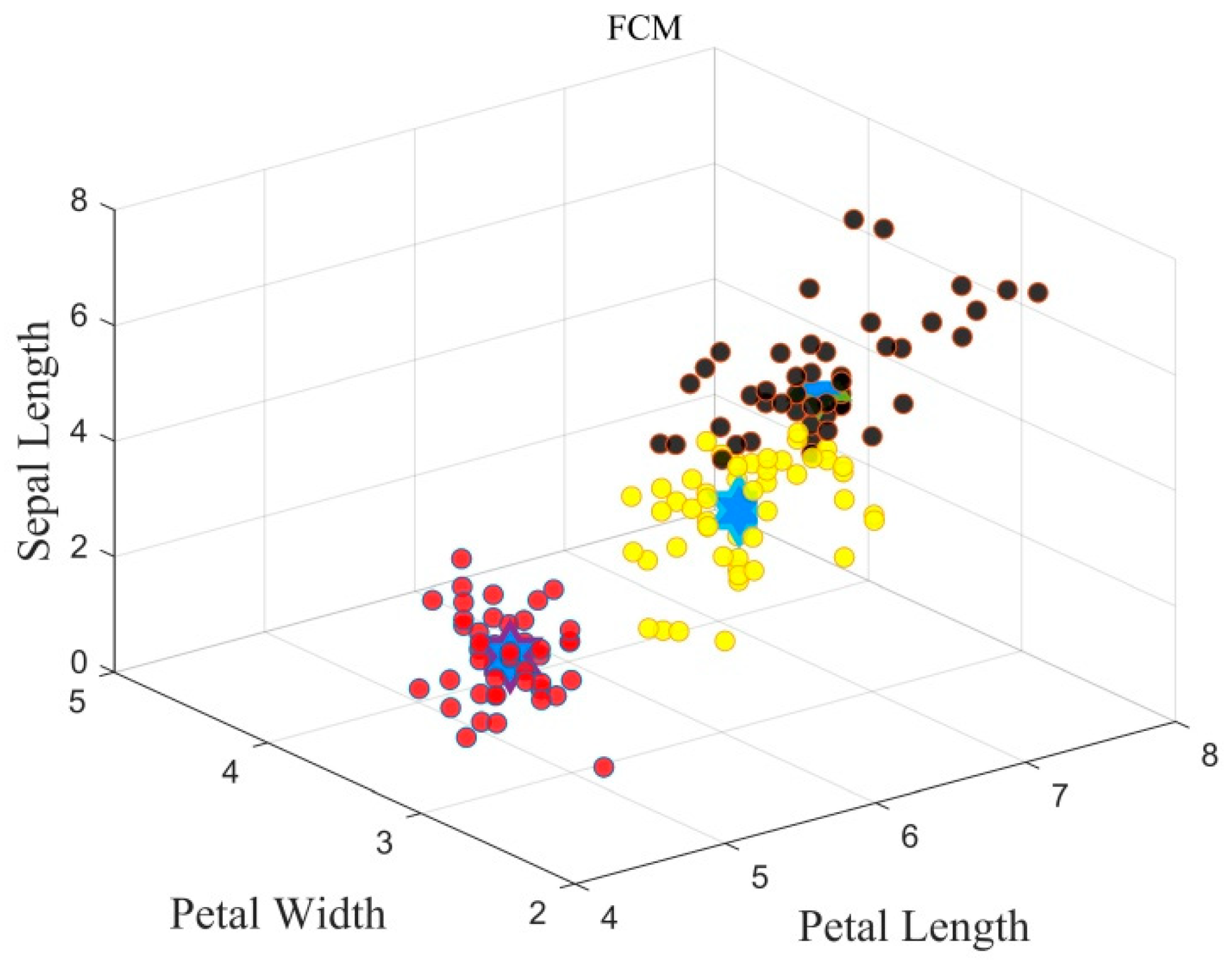
3.1. FCM Theory and Mathematic Basis

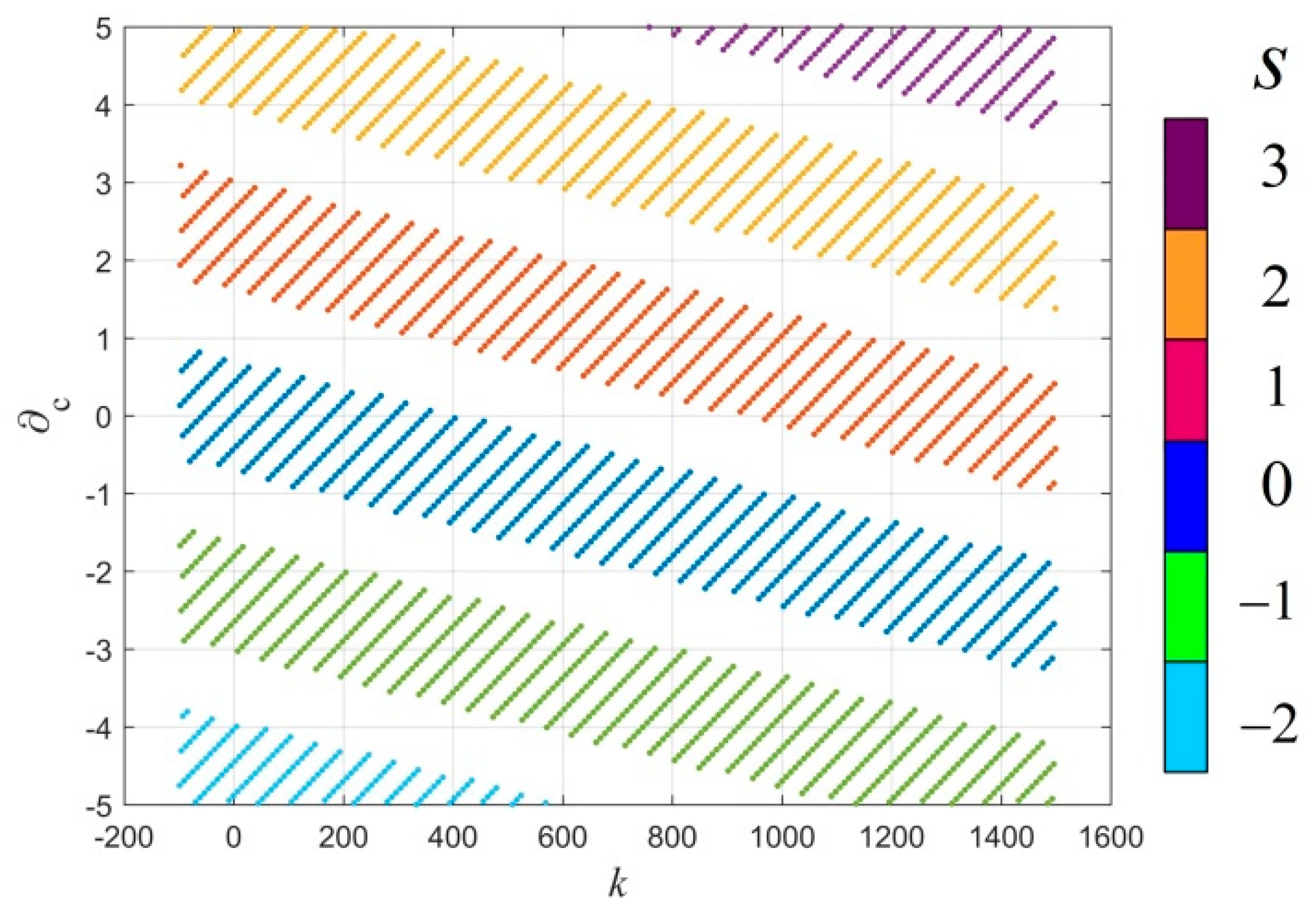
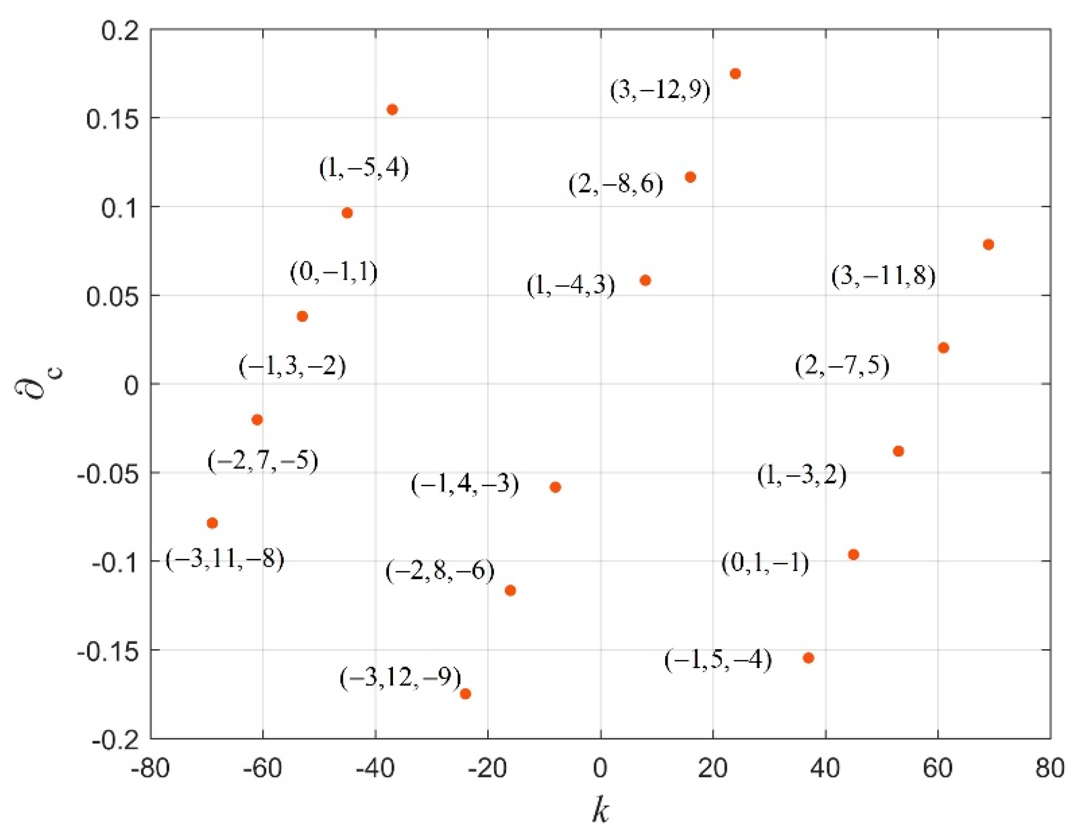
In the present paper, the dataset chosen artificially from triple-frequency combination observations of BDS-3 is defined as $X_n=\{x_1,x_2,\cdots ,x_n\}$ of $n$ objects indexed by $i$ where each object is represented by its corresponding characteristic vector, i.e., $x_i=\{x_{i1},x_{i2},\cdots ,x_{im}\}$. The characteristic vector is composed of $\lambda$, ${\partial }_c$, and $\eta$. In order to eliminate the negative effects of the dimension, the raw dataset is manipulated by a Z-score calculator based on the mean value and standard deviation [24,25].

$c$ is defined as the amount of clusters. And ${\beta }_c$ is defined as the characteristic vector of the corresponding cluster center listed by $j$. Note that the FCM is different from the hard cluster method (HCM) for the underlying idea of the fuzzy partition matrix $U={[u_{ij}]}_{c\times n}$, and $u_{ij}$ is the important index that indicates the proportion of the object with $j^{th}$ cluster center. We define $d_{ij}$ as the Euclidean distance between data $x_i$ and cluster center ${\beta }_j$.

In the FCM, the fuzzy partition matrix is further added as follows

$$J(U,\beta )={\displaystyle \sum _{j=1}^c{\displaystyle \sum _{i=1}^n{(u_{ij})}^m{d}^2(x_i,{\beta }_j)}}$$

(16)

where $m$ is the fuzzy weighting exponent ranging from 1 to 5, and it is regulated as 2 in this paper; $d(x_i,{\beta }_j)$ is the Euclidean distance between data $x_i$ and cluster center ${\beta }_j$, i.e., $d_{ij}=\Vert x_i-{\beta }_j\Vert$. The constraint conditions are as follows

$$u_{ij}\in [0,1],\forall j=1,2,\cdots ,c;\forall i=1,2,\cdots ,n$$

(17)

$${\displaystyle \sum _{j=1}^c{u}_{ij}=1},\forall i=1,2,\cdots ,n$$

(18)

$${\displaystyle 0<\sum _{i=1}^n{u}_{ij}<n},\forall j=1,2,\cdots ,c$$

(19)

The FCM method falls into the category of iterative algorithms. In order to minimize the objective function, the cluster centers and fuzzy partition matrix are updated through the following equations based on the Lagrange method derived by rigorous mathematical proof.

$${\beta }_j=\frac{{\displaystyle \sum _{i=1}^n{(u_{ij})}^m{x}_i}}{{\displaystyle \sum _{i=1}^n{(u_{ij})}^m}}$$

(20)

$$u_{ij}=\frac{1}{{\displaystyle \sum _{k=1}^c{(d_{ij}/d_{kj})}^{(2/(m-1))}}}$$

(21)

During iteration, the cluster centers and fuzzy partition matrix are calculated. The process continues before the new cluster centers change within an error threshold, indicating that the prototypes of cluster centers are stabilized.

Additionally, before implementing the FCM method, the initialization should be finished. The random process is usually used to generate the fuzzy partition matrix and cluster center vectors, causing a severe convergence problem, i.e., falling into the local minimum trap.

3.2. Graph Theory

The clustering method falls into the unsupervised machine-learning algorithm, and there is no prior knowledge about the cluster structure of the dataset, including the number of clusters. Thus, the clustering algorithm executes random initiation conditions, leading to the non-convergence solution or falling into the local optimum.

Taking the selection of triple-frequency combination observations, for example, the first step is to generate a set of cluster centers before implementing the clustering method for almost all algorithms. Additionally, the number of clusters is also unknown, which will be determined by empirical rules or an artificial test. Usually, the maximum number of clusters is less than $\sqrt{n}$.

The present paper proposed a novel approach to calculate the number $c$, called the graph theory model.

Imagine the different data vectors are points in hyper-dimension space. Under specific distance measurement, we determine the distance between any two points. Then, all the data points and the corresponding distance relationship can be treated as undirected weighted graph in graph theory.

A graph $G=(W,E)$ is a pair where $W=(w_1,w_2,\cdots ,w_n)$ is a set of vertices, and $E=\{e_1,e_2,\cdots ,e_s\}$ is a set of edges. The amount of vertices equals the number of data, while the number of edges $s$ is $n(n-1)/2$.

In order to analyze the relationship between every pair of vertices, the Chebyshev distance is the measurement of the different vertices. The definition of the Chebyshev distance is given as follows:

$$\begin{array}{l}D(x_i,x_j)=\max (\left|x_i-x_j\right|)\\ \overline{D}=\frac{{\displaystyle \sum _{i,j=1,i\ne j}^{n}D(x_i,x_j)}}{n(n-1)/2}\end{array}$$

(22)

Further, we define the distance exponent $\lambda =0.6$; edges with distance of more than $\lambda ·\overline{D}$ will be eliminated, where the $\overline{D}$ is the average distance for all the selected edges.

It is impossible and meaningless to incorporate all edges with the graph, especially the ones with too large a distance, which means that they are probably not similar. The underlying idea is to eliminate the extra edges with too large a distance, i.e., more than $\lambda ·\overline{D}$, and to save those edges with limited distance. Then, we can refer to some methods in graph theory, e.g., degree distribution, to analyze the cluster structure.

In graph theory, we can obtain a matrix denoting the relationship between adjacent vertices, called the adjacent matrix, which is given by

$$\begin{array}{l}A=\left[\begin{array}{cccc}{a}_{11}& a_{22}& \cdots & a_{1n}\\ a_{21}& a_{22}& \cdots & a_{2n}\\ ⋮& ⋮& \cdots & ⋮\\ a_{n1}& a_{n2}& \cdots & a_{nn}\end{array}\right],\\ a_{ij}=\{\begin{array}{ll}1,& D\left(x_i,x_j\right)<\lambda \overline{D}\\ 0,& \mathrm{else}\end{array}\end{array}$$

(23)

The degree of $w_i$ is represented as $k_i$, which is actually the number of edges connected with the vertices The degree can be expressed as

$$k_i=a_{ii}^{(2)}$$

(24)

where $a_{ii}^{(2)}$ is the diagonal element of matrix $A^2$.

The vertices with a large degree, and the belonging vertices, will be considered as one cluster. The remaining vertices will update the degree distribution, and then, a similar process will be executed to determine the other cluster centers and their belonging vertices.

Step1: calculate the degree for all vertices.

Step2: reckon the one with the largest degree is the one of the cluster center and eliminate this vertex and its belonging edges.

Step3: calculate the amount of remaining vertices, judge whether the number is less than $0.05n$. If yes, then classify these vertices to the nearest cluster, and if not, return to Step 1.

With the support of the graph theory, we are able to obtain the probable cluster center ${\beta }_0$ and the amount of classes $c$. It is noted that the results are very coarse and merely serve as the initiation of the clustering algorithm. And the initiation results are much better than the random calculation.

3.3. Cluster Indices

3.3.1. CV Based on Granularity Concepts

There are many indices used for cluster validation, among which the DBI, PBM, and DI are the main approaches. The present paper presents a new perspective, called granularity, to examine the clustering validation, which was originally the physical concept being used to depict the measurement of information density. Granularity includes compactness and separation.

Granularity compactness (GC) is similar to the goal function of FCM, which is the average of all the data vectors.

$$GC(c)=\frac{1}{n}{\displaystyle \sum _{j=1}^c{\displaystyle \sum _{i=1}^n{u}_{ij}^m{d}_{ij}^2}},j=1,2,\cdots ,c;i=1,2,\cdots ,n$$

(25)

Granularity separation (GS) depicts the dissimilarity among different classes.

$$GS(c)=\frac{{\displaystyle \sum _{j,k=1;j\ne k}^c{d}_{jk}^2}}{[c(c-1)]/2};j,k=1,2,\cdots ,c;$$

(26)

Hence, the clustering validation function can be expressed as follows:

$$CV(c)=\alpha GC(c)+(1-\alpha )\frac{1}{GS(c)}$$

(27)

The weighting exponent $\alpha$ is used to adjust the compactness index and separation index. The one with the relatively large range will be endowed with small weighting exponent $\alpha$ for better validation results. In general, the weight of GC will be larger than the weight of GS; thus, in the present paper, $\alpha =0.6,1-\alpha =0.4$. Further, we can conclude that smaller $CV(c)$ indicates better clustering results.

3.3.2. PBM Index

Pakhira introduced a new index to evaluate the clustering result, which is defined as [26]

$$V_{\mathrm{PBM}}={(\frac{1}{c}\times \frac{E_1}{J_m}\times D_c)}^2$$

(28)

where $E_1={\displaystyle \sum _{i=1}^n{u}_{ij}\Vert x_i-{\beta }_j\Vert }$; $D_c={\max }_{i,j}^c\Vert {\beta }_i-{\beta }_j\Vert$; $c$ is the number of clusters; $J_m=(U,\beta )={\displaystyle \sum _{i=1}^n{\displaystyle \sum _{j=1}^c{(u_{ij})}^{m_1}\Vert x_i-{\beta }_j\Vert }}$, whereas, $m_1$ here is set to 1.5.

Similar to the GC mentioned in Section 3.3.1, the factor $E_1/J_m$ depicts the overall compactness of the cluster system. What is different is the adoption of $D_c$ depicting the separation distance of the varied cluster center, causing the result that higher PBM indicates better clustering results.

The clustering indices, including CV and PBM, will be used as the evaluation and validation of the proposed clustering method.

3.4. Particle Swarm Optimization (PSO)

The traditional PSO algorithm runs in an intuitive and simple way where each particle utilizes the prior best solution itself and the other particle with global best solution [27]. Ref. [28] claims that the particle swarm technique is more efficient with respect to generic algorithms. Additionally, it was mentioned in ref. [29] that PSO outperforms the differential evolution algorithm.

During the iteration, a certain number of particles are involved to find the best solution. Each particle owns two kinds of properties. One is solution property, referred to as the position matrix p, and the other is mutation property, referred to as the velocity matrix v. Parameters in the optimal control problem constitute the position vector, and every particle can be recognized as a possible solution. The velocity vector includes the information of each particle’s mutation, which helps the particle to find better solution.

Assume $M$ to be the size of the swarm. The position vector and velocity vector can be formulated as p and v. For each particle, the previous best solution property in history will be remarked as $p_{best}$, while the global best solution is $g_{best}$. Obviously, $g_{best}$ is of superiority with respect to $p_{best}$. The PSO follows the equation to search better solutions

$$\begin{array}{l}\{\begin{array}{l}{v}_{i,j}^{t+1}=w{v}_{i,j}^t+c_1{r}_1(p_{best}^t(i,j)-x_{i,j}^t)\\ +c_2{r}_2(g_{best}^t(i,j)-x_{i,j}^t)\\ p_{i,j}^{t+1}=p_{i,j}^t+v_{i,j}^t\end{array},\\ i=1,2,\cdots ,M,j=1,2,\cdots ,m\end{array}$$

(29)

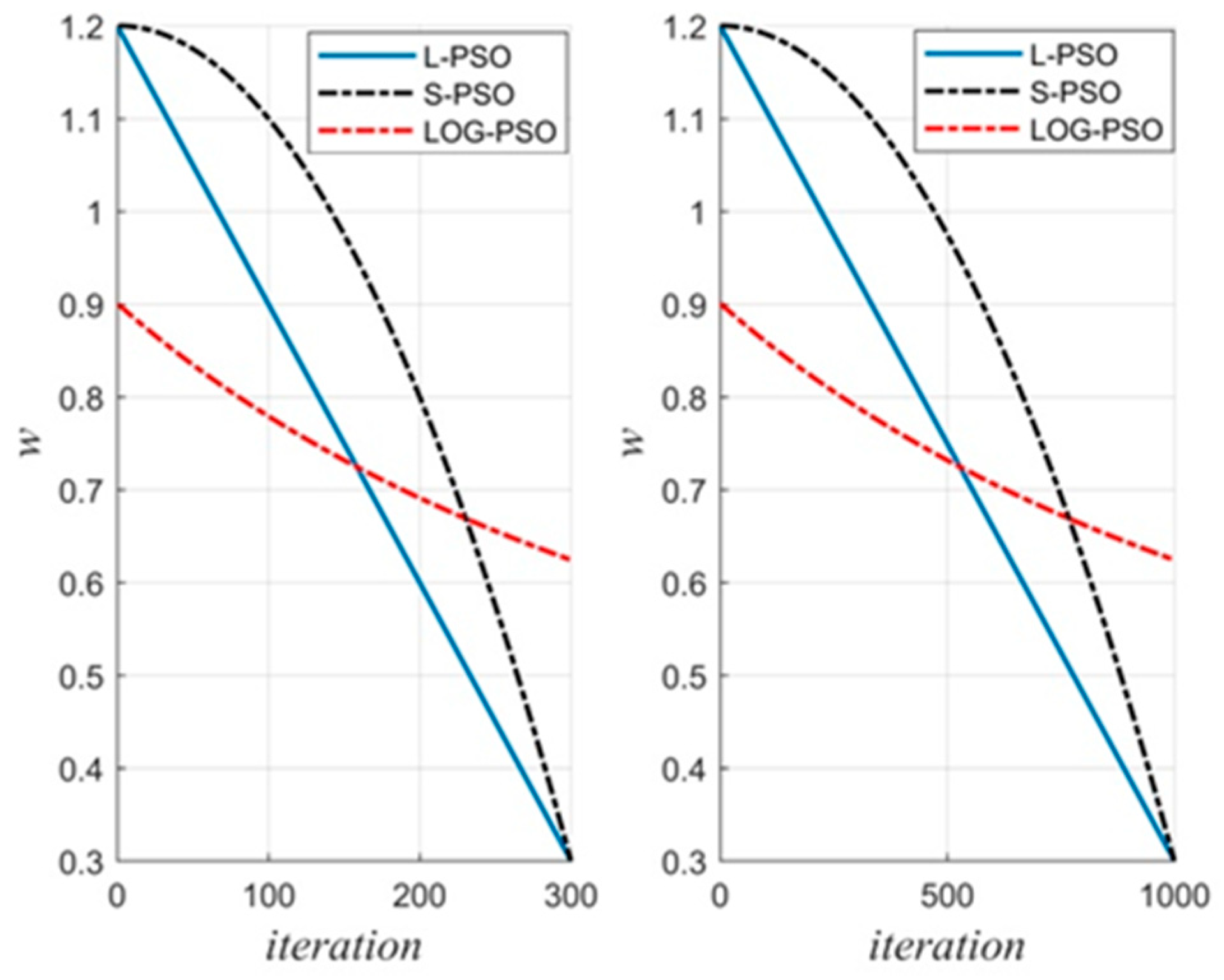
where $v_i^{t+1}$ denotes the $i\mathrm{th}$ particle’s mutation with regard to the parameter in the iteration; $w$ is the inertial weight; $c_1$ and $c_2$ are acceleration coefficients; $r_1,r_2$ are random numbers, which are uniformly distributed in the interval between 0 and 1. More details can be found in ref. [27].

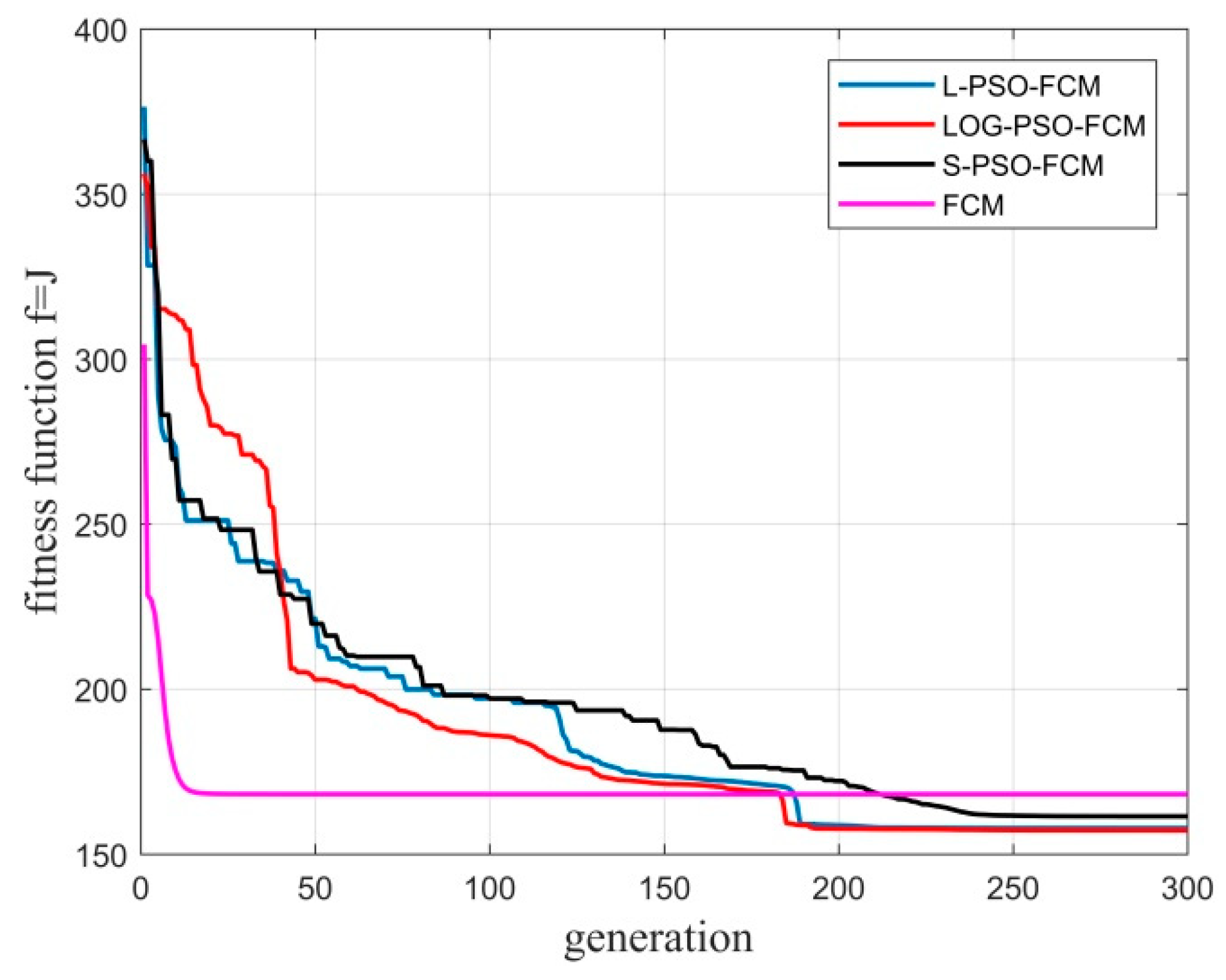
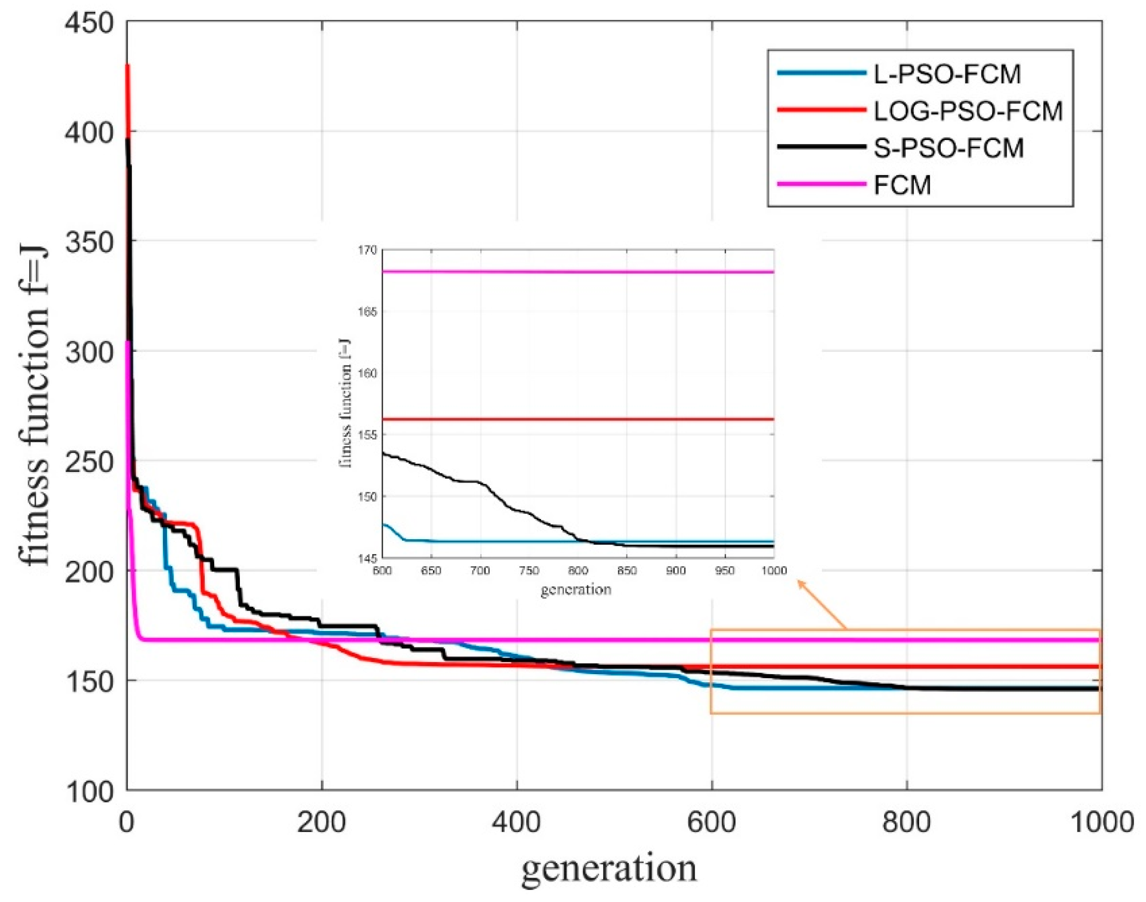
The fitness value is determined by the clustering validation function, according to which the PSO will repeat the application of Equation (29) until the iteration stops. Actually, the fitness function is the parameter that connects the FCM with the PSO method and will be discussed in the remainder of the present paper.

4. Proposed Clustering Algorithms

The present section introduces the hybrid algorithm based on the FCM and improved PSO, combining the merits of these two methods. However, FCM is sensitive to the initial cluster centers and fuzzy partition matrix, tending to fall into the local minimum trap, while the PSO has a strong ability in the global exploration of the optimum.

4.1. Variants of Some Improved PSO

Some variants of PSO were proposed to promote the ability, among which the important one is the variable inertia weight strategy, e.g., Ref. [30]. Inertia weight is a balancing parameter controlling the overall performance of PSO. Large weight indicates better capability in global search, while small weight is of better performance in local exploitation.

Thus, the present paper introduced three kinds of strategies to adjust inertial weight with respect to the iterations.

• Linear inertia weight strategy

The most common improvement is the linear strategy, referred to as L-PSO. It was first introduced by Eberhart to boost the ability of PSO [30]. It has also been mentioned that the performance brought by the linear strategy varied a lot; thus, different kinds of strategies must be experimented for providing an analysis with the specific dataset and background.

Here, one can obtain the linear inertial weight strategy as follows:

$$w(i)=ws-(ws-we)(i/maxgen),i=1,2,\cdots ,maxgen$$

(30)

where $maxgen$ is the max generation; $ws$ and $we$ are set to be constant 1.2 and 0.3.

• Square inertial weight strategy

Similar to the previous section, the square inertial weight strategy, referred to as Square PSO (S-PSO), is expressed as follows:

$$w(i)=ws-(ws-we){(i/maxgen)}^2,i=1,2,\cdots ,maxgen$$

(31)

• Logarithmical inertial weight strategy

Ref. [23] proposed a novel strategy of inertial weight, which has proved to be helpful for balancing the global search and local search capabilities of the particle swarms, referred to as Logarithmical PSO (LOG-PSO) in the present paper. The formulation is as follows:

$$\omega (i)={(\ln (2.98+i/maxgen))}^{-z},i=1,2,\cdots ,maxgen$$

(32)

where $i$ is the current iteration, $z$ is the regulatory factor for fine tuning, e.g., 1.51 by experience.

Set the max generation as 300 and 1000; then, three kinds of inertial weight curves are shown in Figure 1.

Further, the update of three kinds of inertial weight is substituted into Equation (29), as given synthetically by

$$\begin{array}{l}\{\begin{array}{l}{v}_{i,j}^{t+1}=w(k/maxgen)v_{i,j}^t+c_1{r}_1(p_{best}^t(i,j)-x_{i,j}^t)\\ +c_2{r}_2(g_{best}^t(i,j)-x_{i,j}^t)\\ p_{i,j}^{t+1}=p_{i,j}^t+v_{i,j}^t\end{array},\\ i=1,2,\cdots ,M,j=1,2,\cdots ,m,k=1,2,\cdots ,maxgen\end{array}$$

(33)

Let the number of particles be constant $M$, and the position matrix of each particle has a similar format. The size of the position matrix is $c\times m$, where $c$ is the number of clusters obtained by the graph theory model, and $m$ is the dimension of the dataset. Thus, the particle position matrix can be expressed as follows:

$$p(l)=\left[\begin{array}{ccc}{\beta }_{11}& \cdots & {\beta }_{1m}\\ ⋮& \ddots & ⋮\\ {\beta }_{c1}& \cdots & {\beta }_{cm}\end{array}\right],l=1,2,\cdots ,M$$

(34)

Each particle represents a possible solution of cluster centers for the dataset with $m$ dimensions. Once the cluster centers are determined, the fuzzy partition matrix is calculated subsequently according to its membership function mentioned in the FCM method. Every update of particle $p(l)$ means the change of cluster centers followed with Equation (33), where the rule to select the best particle is the fitness function in PSO. Here, the fitness function can be expressed briefly as follows:

$$f(p)=J(U,\beta )$$

(35)

where $J$ is the objective function of the FCM method. Hence, smaller fitness means better clustering results.

4.2. Hybrid Method Based on FCM and PSO

Although FCM is of high efficiency and rigorous mathematic basis, it tends to fall into the local optimum. Thus, an improved PSO algorithm is combined with FCM to utilize the outstanding ability for global searching, whereas in a traditional FCM algorithm and PSO algorithm, the initiation process is usually implemented randomly, causing the initiation sensitivity problem, which is harmful for searching the global optimal solution of the cluster center.

Additionally, the graph theory model provides the cluster number and possible cluster center, which will be used as the initial value.

Specifically, the FCM will be integrated into the framework of the PSO algorithm; thus, the hybrid method, called PSO-FCM, will be strongly integrated together to maintain the merits of both algorithms. The hybrid method provides more advantages over the sensitivity problem occurring in FCM and the local optimum trap by utilizing the optimization framework of the improved PSO.

4.3. Validation of The Proposed Algorithms

Before applying the proposed method to the selection of the optimal triple-frequency combination observation for BDS-3, the proposed clustering method must be verified upon a well-known machine-learning dataset in the present section, called Iris. The running platform is Matlab 2017a, and the CPU is intel i7-11800H 2.3GHz.

The Iris dataset includes 150 samples, which possess four attributes, respectively, i.e., petal length, petal width, sepal length, and sepal width. It contains three classes of the iris plant, which are Iris-setosa, Iris-versicolor, and Iris-virginica, respectively. Since the classes of samples are already known, it is easy to validate the clustering algorithm.

The clustering results derived from the FCM and one of the proposed PSO-FCM methods will be compared with the true clusters provided by the dataset. Without a loss of generality, the S-PSO-FCM is verified in terms of the objective function and cluster centers. The basic clustering results are shown as Figure 2 and Figure 3. The clustering task is easy due to the small number of samples. Additionally, all three kinds of proposed PSO-FCM methods are experimented to search the cluster centers, as shown in

Table 2. Clustering results.

Attributes	True Results	S-PSO-FCM	L-PSO-FCM	LOG-PSO-FCM	FCM
Petal Length	6.58, 5.93, 5.00	6.72, 5.81, 5.00	6.72, 5.81, 5.00	6.72, 5.81, 5.01	6.72, 5.81, 5.01
Petal Width	2.97, 2.77, 3.42	3.07, 2.70, 3.41	3.07, 2.70, 3.41	3.07, 2.70, 3.41	3.07, 2.70, 3.41
Sepal Length	5.55, 4.26, 1.46	5.46, 4.32, 1.50	5.46, 4.32, 1.50	5.46, 4.33, 1.50	5.46, 4.32, 1.50
Sepal Width	2.02, 1.32, 0.24	1.98, 1.38, 0.10	1.98, 1.38, 0.10	1.98, 1.38, 0.26	1.98, 1.38, 0.26

.

It can be concluded that the clustering results obtained from the FCM and S-PSO-FCM are almost the same, except for a little difference in the clustering centers. Hence, the proposed methods are valid and feasible to solve the clustering issue.

5. Results

In this section, firstly, datasets are constructed for BDS-3 B1I, B3I, and B2a, which will be divided into different groups. Secondly, two groups of linearly independent combinations in $S_0$ are selected and analyzed. Thirdly, for group $S_1$, on the basis of proving the clustering advantages of the improved PSO-FCM algorithm based on the public dataset, all combinations are divided into six categories and analyzed. Finally, based on the observation data of short baseline, long baseline, and ultra-long baseline, the success rates of cycle slip detection of the optimal combinations are calculated, and the clustering performance is also studied.

5.1. Datasets Construction

Let $\upsilon =l+m+n$, then, according to the different values of $\upsilon$, $S_{\upsilon }$ represents different groups. Theoretically, $\upsilon$ can be integers, such as 0, ±1, ±2. According to Equations (10) and (13), for given $k$ and ${\partial }_c$, there exists a combination with minimum combined noise based on the principle of minimum noise. In this paper, the traversal search is carried out in the range of $-100\le k\le 1500$ and $-5\le {\partial }_c\le 5$, and they are grouped according to the values of $\upsilon =\pm 2,\pm 1,0,3$. At the same time, the search results are limited in $\eta <100$, as shown in Figure 4.

It can be seen from the above figure that: (a) the searched effective combinations are symmetrically distributed, and the combined ionospheric scale factor gradually decreases with the increase in the number of lanes; (b) for different $\upsilon$, as long as the number of lanes is appropriate, the combined ionospheric delay error can reach zero, that is, there always exists the IF combination; (c) for the same group, the effective data present a banded distribution, that is, there are multiple combinations that meet the same requirements at the same time.

Table 3. The combined wavelength, the combined ionospheric scale factor, and the combined noise amplification factor of typical combinations under different groups.

Group	$\mathit{k}$	Combination	$\mathit{\lambda }$ (m)	${\mathbf{\partial }}_{\mathit{c}}$	$\mathit{\eta }$
$S_{-2}$	−14	(7,−4,−5)	−10.47	−4.55	9.48
	−6	(8,−8,−2)	−24.43	−4.49	11.48
	2	(9,−12,1)	73.31	−4.44	15.03
$S_{-1}$	10	(0,13,−14)	14.66	−2.57	19.10
	410	(5,1,−7)	0.35	−3.05	8.66
	802	(9,−7,−3)	0.18	−3.59	11.78
	1199	(8,6,−15)	0.12	−4.52	18.02
$S_0$	8	(1,−4,3)	18.32	0.058	5.09
	400	(5,−12,7)	0.36	−0.47	14.76
	797	(4,1,−5)	0.18	−1.40	6.48
	1189	(8,−7,−1)	0.12	−1.94	10.67
$S_1$	−10	(0,−13,14)	−14.66	2.57	19.10
	416	(−3,9,−5)	0.35	1.44	10.72
	808	(1,1,−1)	0.18	0.90	1.732
	1208	(6,−11,6)	0.12	0.42	13.89
$S_2$	−2	(−9,12,−1)	−73.31	4.44	15.03
	406	(−3,−4,9)	0.36	4.02	10.29
	806	(2,−16,16)	0.18	3.54	22.71
	1195	(0,1,1)	0.12	2.55	1.41
$S_3$	1203	(−9,26,−14)	0.12	4.41	30.87

shows the combined wavelength, the combined ionospheric scale factor, and the combined noise amplification factor of typical combinations under different groups. It can be seen from the table that the characteristics of typical combinations under different combination coefficients vary greatly, and the long combination wavelength, small combination ionospheric scale factor, and low combination noise amplification factor cannot be uniformly satisfied.

In order to fix the ambiguity under three frequencies, three linearly independent combination coefficients are required. From Figure 4, the appropriate combination is generally selected in the group with small $\upsilon$ and a range close to the $k-{\partial }_c$ plane, such as $S_0$. However, in $S_0$, the sum of combination coefficients is zero, so there are only two linearly independent combinations at most. At this point, the last combination should be selected from $S_{\pm 1}$. Due to the symmetrical distribution, $S_1$ is analyzed in the next section.

According to the previous search results, all data in $S_0$ and $S_1$ are used as the dataset to test the performance of the proposed algorithms.

5.2. Group of BDS-3 Triple-Frequency Combinations

5.2.1. The First Group S₀

As mentioned earlier, there are only two linearly independent combinations in $S_0$. Firstly, the first combination selects the combination when the combined ionospheric scale factor and the number of lanes are close to 0. The origin area is enlarged in Figure 5. Additionally,

Table 4. Information of all combinations in Figure 5.

$\mathit{k}$	Combination	$\mathit{\lambda }$ (m)	${\mathbf{\partial }}_{\mathit{c}}$	$\mathit{\eta }$
−69	(−3,11,−8)	−2.13	−0.08	13.93
−24	(−3,12,−9)	−6.11	−0.17	15.30
−61	(−2,7,−5)	−2.40	−0.02	8.83
−16	(−2,8,−6)	−9.16	−0.12	10.20
−53	(−1,3,−2)	−2.77	0.04	3.74
−8	(−1,4,−3)	−18.33	−0.06	5.10
37	(−1,5,−4)	3.96	−0.15	6.48
−45	(0,−1,1)	−3.26	0.10	1.41
45	(0,1,−1)	3.26	−0.10	1.41
−37	(1,−5,4)	−3.96	0.15	6.48
8	(1,−4,3)	18.33	0.06	5.10
53	(1,−3,2)	2.77	−0.04	3.74
16	(2,−8,6)	9.16	0.12	10.20
61	(2,−7,5)	2.40	0.02	8.83

lists the specific information of all combinations in the figure.

As can be seen from Figure 5 and Table 4, (1,−4,3) and (−1,4,−3) have longer combined wavelengths, smaller combined ionospheric scale factor and lanes. The two combinations are symmetrical to each other. In this paper, (1,−4,3) is selected as the first combination. At the same time, all points on the straight line in Figure 5 are linearly correlated, so the second combination is selected at the adjacent points.

When using the matrix change method to solve the ambiguity, the ionospheric delay error can be ignored in the short baseline scenario, and the influence of observation noise is very important. In the long baseline scenario, the data smoothing method must be adopted, and the influence of the ionospheric delay error and observation noise is very important. Considering the symmetry, in the short baseline scenario, the combination that the number of lanes is close to 0 is preferred. As can be seen from Table 4, the noise amplification factor of (0,1,−1) is small and can be selected as the second combination in the short baseline scene. Similarly, in the long baseline scenario, the combination that the combined ionospheric scale factor is close to 0 is preferred. As can be seen from Table 4, the noise amplification factor of (1,−3,2) is small and can be selected as the second combination in the long baseline scene.

5.2.2. The Second Group S₁

Clustering Research

The present section is divided into two parts: the clustering results of the original FCM and the three proposed variants of the PSO-FCM method with varied inertial weight will be compared, and better clustering results will be employed for selecting the optimal combination of triple frequency.

The dataset includes 688 available samples with three attributes, respectively, i.e., wavelength, ionospheric delay coefficient, and noise amplification factor. The involved algorithms are performed with 300 iterations and 1000 iterations to survey the effect of the iterations.

The populations for the three variants of the PSO-FCM algorithms are set to 100 uniformly, and other parameters are regulated following previous equations.

The iteration curves are shown in Figure 6 and Figure 7.

The Y-axis is the fitness function $J$, while the X-axis is the iterations. In the beginning phase of the four kinds of algorithms, the fitness values are very large, which uniformly indicates the initial cluster centers derived from the graph theory still possess the potential to promote. As mentioned before, the graph theory model is an auxiliary approach to determine the very coarse initial cluster centers, aiming mostly to help the subsequent algorithms to obtain better results than the traditional FCM algorithm where the initial value is calculated randomly.

What is intuitive is that the initial fitness values for the three variants of the PSO-FCM algorithms are the same, which differ from the FCM. Meanwhile, what is non-intuitive is that even though FCM has a relatively lower fitness value, i.e., better clustering results, it is finally defeated by the other three algorithms after about 200 iterations. The present paper concludes that the proposed approach to use the graph theory for initiation is feasible, which plays a more feasible role in the initiation process.

Moreover, the fitness value of FCM descends very quickly within the first 20 iterations, whereas in the later iterations, it holds the same level, indicating there is no improvement change of the cluster centers. It can be concluded that the FCM falls into the local minimum trap after about 20 iterations. The update of the clustering prototype matrix and the fuzzy partition matrix is invalid to eliminate the local optimum and thus unable to search better cluster centers.

While the FCM’s velocity to find a better solution is much faster than the other three algorithms in the early stage, the other three algorithms possess considerable ability to search global optimum solutions.

The other three algorithms begin to exceed FCM after about 180 iterations, and during most iterations, the LOG-PSO-FCM and L-PSO-FCM possess better results than the S-PSO-FCM, while, finally, the S-PSO-FCM achieves the best fitness value after about 850 iterations, as shown in Figure 7.

In order to evaluate the performance of the proposed methods, the clustering results in terms of several indices are listed in

Table 5. Clustering indices of different algorithm results (best results are highlighted in bold).

Algorithm	Iterations	PBM	CV	$\mathit{J}$
S-PSO-FCM	300	186.2225	0.2086	165.2535
	1000	224.5406	0.1944	143.6415
L-PSO-FCM	300	179.3561	0.2156	157.2448
	1000	220.9347	0.1961	145.7575
LOG-PSO-FCM	300	207.1792	0.2049	155.1127
	1000	212.6527	0.2009	150.2784
FCM	300	33.5642	0.3600	168.1527
	1000	33.5644	0.3600	168.1527

. As mentioned before, $J$ is the objective function value, while the PBM and CV are synthesized indices with effective clustering validity ability.

Larger values of PBM indicate better clustering results, while smaller values of CV mean better results. All algorithms are tested over 300 iterations and 1000 iterations, and the involved results are consistent with the fitness curves above. It can be seen that the FCM is defeated by all the proposed methods.

The best scores are marked in bold, namely the S-PSO-FCM, achieving the lowest $J$, smallest CV, and largest PBM. Investigating the results in terms of the indices listed in Table 5 strongly verifies the correctness of the clustering results for the consistency in indices and avoids misjudgments as much as possible.

It can be concluded that the three variants of the proposed algorithms have better performance than the traditional FCM method in terms of comprehensive clustering indices. Not only the PSO strategy but also the initialization method, i.e., the graph theory, are responsible for the good results. Note that the coordination of these two parts contributes to the proposed algorithm. Thus, the two parts are both indispensable and important.

Clustering Results for S₁

In order to ensure the linear independence of the three combinations, the third combination needs to be selected in $S_1$. In this paper, the improved PSO-FCM algorithms are selected to cluster all combinations in the range $-98\le k\le 1499$. The clustering results are shown in Figure 8. For comparison, the clustering results of the FCM algorithm are also given.

Corresponding to the clustering results under different algorithms in the figure, all combinations are classified according to the following characteristics.

(1)

The combined wavelength is long, and the combined noise amplification factor is small, which is suitable for ambiguity resolution under short baseline.

(2)

The combined wavelength and the combined ionospheric scale factor are relatively moderate, and the combined noise amplification factor is small, which belongs to the optional combination in a specific scene.

(3)

The combined wavelength is short, but the combined ionospheric scale factor and the combined noise amplification factor are small, which is suitable for ambiguity resolution under long baseline.

(4)

The combined wavelength is long, but the combined noise amplification factor is too large, which is different from the first kind and belongs to the bad cluster.

(5)

The combined wavelength and the combined ionospheric scale factor are relatively moderate, but the combined noise amplification factor is large, which belongs to the bad cluster.

(6)

The combined ionospheric scale factor is small, but the combined noise amplification factor is large, which is different from the third kind and belongs to the bad cluster.

Among the above six categories, the first category is preferred in the short baseline scenario, and the third category is preferred in the long baseline and ultra-long baseline scenarios. The centers of the six categories are indicated by five pointed stars in Figure 8.

5.3. Algorithm Performance under Different Baselines

In order to study the performance of optimal combinations under different algorithms, the measured data under the short baseline, the long baseline, and the ultra-long baseline scenarios are selected to carry out ambiguity resolution. The data under the short baseline scene are provided by the China University of Mining and Technology (Xuzhou). The data under the long baseline scenario are from the fixed station under the above short baseline scenario and the WUH2 station. The data under the ultra-long baseline scenario are from the SGOC and WUH2 stations. The specific information under the three scenarios is listed in

Table 6. Information under different baseline scenarios.

Baseline Type	Station	Position	Sampling Interval/s	Date	Location
short	——	~40.31°N, ~116.63°E	1	15 July 2021	Beijing, China
long	——	~40.31°N, ~116.63°E	1	15 July 2021	Beijing, China
	WUH2	114.36°N, 30.53°E			Wuhan, China
ultra-long	WUH2	114.36°N, 30.53°E	1	27 August 2021	Wuhan, China
	SGOC	6.89°N, 79.87°E			Sri Lanka

. In order to eliminate the influence of the receiver clock error, satellite clock error, and other errors, the triple-difference data of BDS-3 C27 and C39 at B1I, B3I, and B2a are used in the short baseline and long baseline scenarios, respectively, while the triple-difference data of BDS-3 C37 and C40 are studied in the ultra-long baseline scenario. Cycle slips are eliminated from the measured data in the three scenarios.

5.3.1. The Short Baseline Scenario

As mentioned above, according to the optimal combination under the short baseline scene given by the S-PSO-FCM, L-PSO-FCM, LOG-PSO-FCM, and FCM algorithms, the combined triple-difference ambiguities under different epochs are calculated, as shown in Figure 9. By comparing the proportion of epochs with the differencing values over 0.5 cycles, the success rate of the combined triple-difference ambiguity repair can be obtained.

Table 7. The success rates of the combined triple-difference ambiguity repair calculated by the four algorithms.

Baseline	Algorithm	Combination	$\mathit{\lambda }$ (m)	${\mathbf{\partial }}_{\mathit{c}}$	$\mathit{\eta }$	Success Rate
short	S-PSO-FCM	(−5,9,−3)	3.67	2.09	10.72	99.3%
	L-PSO-FCM	(−5,10,−4)	1.73	2.00	11.87	97.9%
	LOG-PSO-FCM	(−5,11,−5)	1.13	1.90	13.08	94.7%
	FCM	(−5,12,−6)	0.84	1.80	14.32	89.8%
long	S-PSO-FCM	(−2,1,2)	0.60	1.89	3.00	94.9%
	L-PSO-FCM	(−1,1,1)	0.34	1.56	1.73	74.5%
	LOG-PSO-FCM	(−2,2,1)	0.51	1.79	3.00	68.6%
	FCM	(−1,0,2)	0.38	1.65	2.24	66.1%
ultra-long	S-PSO-FCM	(3,−1,−1)	0.13	0.44	3.32	12.8%
	L-PSO-FCM	(3,0,−2)	0.13	0.35	3.61	14.3%
	LOG-PSO-FCM	(3,1,−3)	0.12	0.25	4.36	6.1%
	FCM	(3,2,−4)	0.12	0.15	5.39	2%

lists the success rates of the combined triple-difference ambiguity repair calculated by the four algorithms in the short baseline scenario. It can be seen from the table that the success rate of (−5,9,−3) optimized by the S-PSO-FCM algorithm is the highest, reaching 99.3%, which is better than 97.9% of the L-PSO-FCM algorithm and 94.7% of the LOG-PSO-FCM algorithm. The three improved PSO-FCM algorithms are all better than the FCM algorithm. This proves the superiority of the improved algorithms proposed in this paper under the short baseline scenario.

5.3.2. The Long Baseline Scenario

Figure 10 shows the combined triple-difference ambiguities calculated by the four algorithms under different epochs. The success rates are also listed in Table 7. It can be seen that the success rate of (−2,1,2) optimized by the S-PSO-FCM algorithm is the highest, reaching 94.9%, which is much higher than the other three algorithms. It illustrates that the S-PSO-FCM algorithm can achieve the best effect in the long baseline scenario.

5.3.3. The Ultra-Long Baseline Scenario

Under the ultra-long baseline scenario, due to the long distance between the observation stations, there are few effective epochs that can be observed by the two satellites at the same time. Figure 11 shows the combined triple-difference ambiguity calculated by the four algorithms in different epochs under the ultra-long baseline scenario. The success rates are listed in Table 7 as well. It can be seen from the table that the success rates of the four algorithms are all less than 15%. This indicates that the ultra-long baseline scenario is not suitable for using the linear combination triple-difference method to repair and fix the ambiguity.

6. Discussion

Actually, once the combination is confirmed, it can be directly used without repeated selection. However, it is essential to study the similarity of the many different combinations. Moreover, on the one hand, GNSS is moving in the direction of frequency tunability, and the frequencies can be changed according to the actual requirement. On the other hand, embedding adaptive screening procedures in positioning programs can also help improve program adaptability.

Obviously, a better application of the clustering method will be conducive for selecting better triple-frequency observations. Consistent with the literature, this research found that the improved versions of the cluster method can achieve better clustering indices than the traditional FCM algorithm. We assume several reasons for the better performance of the proposed methods.

The first and most important point is the outstanding global optimization ability of the PSO algorithm, where the improvements underlying the present study expanded this advantage. The good agreements found in Figure 7 and Table 5 will give a strong support for the first point, where the fitness values of FCM remain constant during most iterations, and the corresponding clustering indices are almost identical with respect to 300 and 1000 iterations, indicating that the implementation of the conventional FCM falls into the local optimization at a very early stage and loses gradient to improve performance. A possible explanation for these results may be the lack of sufficient gradient to eliminate the local optimum trap.

In contrast, the three variants of PSO are able to achieve a better global search, thus eliminating the local optimum trap. Observations of the fitness curves in Figure 6 and Figure 7 may reveal a possible explanation for this; the unique global search strategy in PSO gives the FCM the ability to escape from the local optimum trap, so that the fitness values will be better updated compared to the traditional FCM approach.

Among the three variants of PSO, different inertial weights may reflect the ability to adjust global and local search. It is not easy to find a suitable inertial weight value for all generations. The present study provides three appropriate adjustment strategies to investigate the effect of inertia weights. The results demonstrate the S-PSO-FCM method is best in terms of the fitness values and all clustering indices, which suggests that relatively high inertial weights in the early stage and smaller values in the subsequent phase are associated with better results.

The second point is the robust performance. To the best knowledge of the authors, there is no corresponding study that has ever applied the graph theory in the initiation of the clustering algorithm. Note that this study uses the Chebyshev distance to generate the initiation vertices, and some specific details of this method are still worth further research. This is a stride from the previous random initiation process, which uses none of the prior knowledge of the dataset. To some extent, this method guarantees the robust performance of the subsequent realization of the clustering algorithm.

The generalization ability was demonstrated in this study. For the results of the public dataset, it can be seen from Figure 6 and Figure 7 and Table 7 that the fitness of the FCM algorithm in the early stage of the iteration is lower than that of the three improved algorithms, which indicates a better clustering performance. However, with the increase in the number of iterations, the clustering performance of the three improved algorithms is better.

Specifically, the PBM, CV, and $J$ of the S-PSO-FCM algorithm are separately 224.54, 0.19, and 143.64 after iterating 1000 times, which is better than the other three algorithms. Additionally, the PBM, CV, and $J$ of the three improved algorithms are all better than the FCM algorithm.

When the proposed method is applied to the BDS-3 measured data, it can be seen from Table 7 that in the short baseline scenario, the success rates of the combined triple-difference ambiguity repair of the S-PSO-FCM, L-PSO-FCM, and LOG-PSO-FCM algorithms are much higher, which are separately improved by 9.5%, 8.1%, and 4.9% compared with the FCM algorithm. In the long baseline scenario, they are improved by 28.8%, 8.4%, and 2.5%, respectively. In the ultra-long baseline scenario, they are separately improved by 10.8%, 12.3%, and 4.1%, but the overall success rates are all less than 15%.

On the one hand, this shows that the baseline length significantly affects the ambiguity restoration and thus the differential localization accuracy. On the other hand, this illustrates that the algorithm performance of the three improved algorithms and the impact on the optimization of the triple-frequency combination are different. Furthermore, these demonstrate the effectiveness of the three improved algorithms in optimizing the combinations of triple-frequency observations and their superiority compared to the traditional FCM algorithm.

7. Conclusions

This study reports some valuable concepts to boost the ability of the traditional FCM method, i.e., the graph theory with Chebyshev distance and advanced variants of the PSO method, and the improved versions of FCM show better performance in terms of various clustering indices. To the best knowledge of the authors, few of these concepts were found in the literature on the application to clustering methods, or the optimal selection of triple-frequency combinations. So, it is also an advance in the application of intelligent algorithms in satellite navigation.

In conclusion, the performance of the improved PSO-FCM algorithms proposed in this paper is better than the FCM algorithm under the public dataset and the BDS-3 measured data, which proves the superiority of the proposed algorithms. However, there still exist some problems that should be further studied. Three scenarios are roughly selected in this paper. The situation of slightly larger sampling time interval and higher ionospheric activity should be considered in the following research.

References

1. Chang, G.; Xu, T.; Yao, Y.; Wang, Q. Adaptive Kalman filter based on variance component estimation for the prediction of ionospheric delay in aiding the cycle slip repair of GNSS triple-frequency signals. J. Geod. 2018, 92, 1241–1253. [Google Scholar] [CrossRef]
2. Huang, L.; Lu, Z.; Xiao, Z.; Ren, C.; Song, J.; Li, B. Suppression of Jammer Multipath in GNSS Antenna Array Receiver. Remote Sens. 2022, 14, 350. [Google Scholar] [CrossRef]
3. Zhao, J.; Hernández-Pajares, M.; Li, Z.; Wang, L.; Yuan, H. High-rate Doppler-aided cycle slip detection and repair method for low-cost single-frequency receivers. GPS Solut. 2020, 24, 1–13. [Google Scholar] [CrossRef]
4. Dai, P.; Xing, J.; Ge, Y.; Yang, X.; Qin, W.; Dong, Y.; Zhang, Z. The Effect of BDS-3 Time Group Delay and Differential Code Bias Corrections on Positioning. Appl. Sci. 2020, 11, 104. [Google Scholar] [CrossRef]
5. De Lacy, M.C.; Reguzzoni, M.; Sansò, F. Real-time cycle slip detection in triple-frequency GNSS. GPS Solut. 2012, 16, 353–362. [Google Scholar] [CrossRef]
6. Cocard, M.; Bourgon, S.; Kamali, O.; Collins, P. A systematic investigation of optimal carrier-phase combinations for modernized triple-frequency GPS. J. Geod. 2008, 82, 555–564. [Google Scholar] [CrossRef]
7. Shi, C.; Tian, Y.; Zheng, F.; Hu, Y. Accounting for Signal Distortion Biases for Wide-Lane and Narrow-Lane Phase Bias Estimation with Inhomogeneous Networks. Remote Sens. 2022, 14, 191. [Google Scholar] [CrossRef]
8. Tian, R.; Fan, X.; Dai, Y.; Sun, X.; Dong, X. Optimal triple-frequency combination observations for BDS-3 derived from a modified kernel-based fuzzy C-means clustering algorithm. Syst. Eng. Electron. 2020, 42, 686–697. [Google Scholar]
9. Bezdek, J.C.; Ehrlich, R.; Full, W. FCM: The fuzzy c-means clustering algorithm. Comput. Geosci. 1984, 10, 191–203. [Google Scholar] [CrossRef]
10. Kesemen, O.; Tezek, O.; Özkul, E. Fuzzy c-means clustering algorithm for directional data (FCM4DD). Expert Syst. Appl. 2016, 58, 76–82. [Google Scholar] [CrossRef]
11. Verma, H.; Agrawal, R.K.; Sharon, A. An improved intuitionistic fuzzy c-means clustering algorithm incorporating local in-formation for brain image segmentation. Appl. Soft Comput. 2016, 46, 543–557. [Google Scholar] [CrossRef]
12. Meng, F.; Li, S.; Pan, Z.; Sun, Y.; Li, P. Optimization and selection of BDS triple-frequency combination observations based on a weighted fuzzy C-means algorithm. J. Natl. Univ. Def. Technol. 2019, 41, 92–98. [Google Scholar]
13. Xing, Z.; Wang, Z.; Wu, Y. Choice of carrier phase combined observation of GPS using fuzzy cluster. Geomat. Inf. Sci. Wuhan Univ. 2006, 31, 23–26. [Google Scholar]
14. Graves, D.; Pedrycz, W. Fuzzy c-means, gustafson-kessel fcm, and kernel-based fcm: A comparative study. In Analysis and Design of Intelligent Systems Using Soft Computing Techniques; Springer: Berlin/Heidelberg, Germany, 2007; pp. 140–149. [Google Scholar]
15. Huang, L.; Song, L.; Liu, X. Optimization and selection of GPS triple-carries phase combination observations based self-adaptive clustering algorithm. J. Geod. Geodyn. 2011, 31, 99–102. [Google Scholar]
16. He, W.; Tao, T.; Wang, Z. Selection on improved fuzzy C-means algorithm of BeiDou triple-frequency combination observations. Chin. Space Sci. Technol. 2014, 34, 24–30. [Google Scholar]
17. Wu, Z.-D.; Xie, W.-X.; Yu, J.-P. Fuzzy C-means clustering algorithm based on kernel method. J. Xidian Univ. (Nat. Sci.) 2004, 31, 49–54. [Google Scholar] [CrossRef]
18. Kuo, R.; Lin, T.; Zulvia, F.; Tsai, C. A hybrid metaheuristic and kernel intuitionistic fuzzy c-means algorithm for cluster analysis. Appl. Soft Comput. 2018, 67, 299–308. [Google Scholar] [CrossRef]
19. Dardanelli, G.; Maltese, A.; Pipitone, C.; Pisciotta, A.; Brutto, M.L. NRTK, PPP or Static, That Is the Question. Testing Different Positioning Solutions for GNSS Survey. Remote Sens. 2021, 13, 1406. [Google Scholar] [CrossRef]
20. Zhao, D.; Roberts, G.W.; Hancock, C.M.; Lau, L.; Bai, R. A triple-frequency cycle slip detection and correction method based on modified HMW combinations applied on GPS and BDS. GPS Solut. 2019, 23, 22. [Google Scholar] [CrossRef]
21. Li, P.; Jiang, X.; Zhang, X.; Ge, M.; Schuh, H. Kalman-filter-based undifferenced cycle slip estimation in real-time precise point positioning. GPS Solut. 2019, 23, 1–13. [Google Scholar] [CrossRef]
22. Liu, W.; Jin, X.; Wu, M.; Hu, J.; Wu, Y. A New Real-Time Cycle Slip Detection and Repair Method under High Ionospheric Activity for a Triple-Frequency GPS/BDS Receiver. Sensors 2018, 18, 427. [Google Scholar] [CrossRef] [PubMed] [Green Version]
23. Zhang, J.; Ma, Z. Hybrid Fuzzy Clustering Method Based on FCM and Enhanced Logarithmical PSO (ELPSO). Comput. Intell. Neurosci. 2020, 2020, 1–12. [Google Scholar] [CrossRef] [PubMed] [Green Version]
24. Zhang, D.-Q.; Chen, S.-C. Clustering Incomplete Data Using Kernel-Based Fuzzy C-means Algorithm. Neural Process. Lett. 2003, 18, 155–162. [Google Scholar] [CrossRef]
25. Lin, K.-P. A Novel Evolutionary Kernel Intuitionistic Fuzzy $C$ -means Clustering Algorithm. IEEE Trans. Fuzzy Syst. 2014, 22, 1074–1087. [Google Scholar] [CrossRef]
26. Pakhira, M.K.; Bandyopadhyay, S.; Maulik, U. Validity index for crisp and fuzzy clusters. Pattern Recognit. 2004, 37, 487–501. [Google Scholar] [CrossRef]
27. Eberhart, R.; Kennedy, J. A new optimizer using particle swarm theory. In Proceedings of the Sixth International Symposium on Micro Machine and Human Science, Nagoya, Japan, 4–6 October 1995; pp. 39–43. [Google Scholar]
28. Angeline, P.J. Evolutionary optimization versus particle swarm optimization: Philosophy and performance differences. In Proceedings of the International Conference on Evolutionary Programming, San Diego, CA, USA, 25–27 March 1998; pp. 601–610. [Google Scholar] [CrossRef]
29. Eberhart, R.C.; Shi, Y. Comparison between genetic algorithms and particle swarm optimization. In Proceedings of the International Conference on Evolutionary Programming, San Diego, CA, USA, 25–27 March 1998; pp. 611–616. [Google Scholar] [CrossRef]
30. Kennedy, J.; Eberhart, R. Particle swarm optimization. In Proceedings of the ICNN’95-International Conference on Neural Networks, Perth, WA, Australia, 27 November–1 December 1995; Volume 4, pp. 1942–1948. [Google Scholar]
Figure 1. Inertial weight profile with respect to iterations.
Remotesensing 14 03713 g001
Figure 2. Standard dataset results from FCM. (The black solid dot denotes the Iris-verginica. The red solid dot denotes the Iris-setosa, and the yellow solid dot denotes the Iris-versicolor.)
Remotesensing 14 03713 g002
Figure 3. Standard dataset results from S-PSO-FCM. (The black solid dot denotes the Iris-verginica. The red solid dot denotes the Iris-setosa, and the yellow solid dot denotes the Iris-versicolor.)
Remotesensing 14 03713 g003
Figure 4. Triple-frequency combinations obtained by search ( η < 100 ).
Remotesensing 14 03713 g004
Figure 5. Partial enlarged drawing of the origin area in S 0 .
Remotesensing 14 03713 g005
Figure 6. Fitness curves for 300 generations.
Remotesensing 14 03713 g006
Figure 7. Fitness curves for 1000 generations.
Remotesensing 14 03713 g007
Figure 8. Clustering results with respect to different algorithms. (The data samples in different classes and the corresponding cluster centers are shown. The existing differences in Table 4 will be embodied through this figure—not very fiercely though. The overall clustering results are very close).
Remotesensing 14 03713 g008aRemotesensing 14 03713 g008b
Figure 9. Differencing values calculated by four algorithms under the short baseline scenario.
Remotesensing 14 03713 g009
Figure 10. Differencing values calculated by four algorithms under the long baseline scenario.
Remotesensing 14 03713 g010
Figure 11. Differencing values calculated by four algorithms under the ultra-long baseline scenario.
Remotesensing 14 03713 g011