Article

Energy-Efficient Cooperative MIMO Formation for Underwater MI-Assisted Acoustic Wireless Sensor Networks

1
School of Information and Control Engineering, China University of Mining and Technology, Xuzhou 221116, China
2
Xuzhou Engineering Research Center of Intelligent Industry Safety, and Emergency Collaboration, Xuzhou 221116, China
3
School of Electronic Engineering, Jiangsu Ocean University, Lianyungang 222005, China
4
Jiangsu Automation Research Institute, Lianyungang 222061, China
*
Author to whom correspondence should be addressed.
Remote Sens. 2022, 14(15), 3641; https://doi.org/10.3390/rs14153641
Submission received: 23 June 2022 / Revised: 23 July 2022 / Accepted: 27 July 2022 / Published: 29 July 2022
(This article belongs to the Special Issue Underwater Communication and Networking)

Abstract

:
The energy problem has become one of the critical factors limiting the development of underwater wireless sensor networks (UWSNs), and cooperative multiple-input–multiple-output (MIMO) technology has shown advantages in energy saving. However, the design of energy-efficient cooperative MIMO techniques does not consider the actual underwater environment, such as the distribution of nodes. Underwater magnetic induction (MI)-assisted acoustic cooperative MIMO WSNs as a promising scheme in throughput, signal-to-noise ratio (SNR), and connectivity have been demonstrated. In this paper, the potential of the networks to reduce energy consumption is further explored through the joint use of cooperative MIMO and data aggregation, and a cooperative MIMO formation scheme is presented to make the network more energy efficient. For this purpose, we first derive a mathematical model to analyze the energy consumption during data transmission, considering the correlation between data generated by nodes. Based on this model, we proposed a cooperative MIMO size optimization algorithm, which considers the expected transmission distance and transmission power constraints. Moreover, a competitive cooperative MIMO formation algorithm that jointly designs master node (MN) selection and cooperative MIMO size can improve energy efficiency and guarantee the connectivity of underwater nodes and surface base station (BS). Our simulation results confirm that the proposed scheme achieves significant energy savings and prolongs the network lifetime considerably.

1. Introduction

Nowadays, with the skyrocketing demands for underwater and marine exploitation, researchers have set out to explore more possibilities of applying underwater wireless sensor networks (UWSNs) [1,2,3]. This requires not only reliable and real-time communications within underwater sensor nodes, but also long-range, high-throughput, and reliable communication between the underwater sensor nodes and the remote surface base station (BS) [4]. The traditional underwater networks based on acoustic signals cannot meet the above requirements [5,6]. Additionally, since battery-constrained nodes determine the network lifetime, energy conservation and energy efficiency are also critical factors in the design of new UWSNs [7].
In contrast to single-input–single-output (SISO) systems, multiple-input–multiple-output (MIMO) systems employ more than one antenna at both the transmitter and the receiver. Thus, MIMO provides two main advantages for wireless communications: spatial diversity gain and spatial multiplexing gain, which can satisfy the long-range, high-throughput, and reliable requirements of UWSNs [8]. However, the large wavelength makes it challenging to place multiple acoustic transducers on a single underwater device to guarantee spatial independence. Under the premise of the perfect synchronization of nodes, the cooperative MIMO technique can achieve MIMO communication by grouping multiple devices as virtual antenna arrays [9]. Many works have focused on theoretical feasibility analysis of underwater distributed acoustic MIMO communications. However, the work on implementing cooperative MIMO communications in underwater environments is very limited, since it is challenging to synchronize the received signal [10,11].
The synchronization strategies for distributed transmitters can be classified as close-loop synchronization and open-loop synchronization. However, due to the complex and time-delayed acoustic channel between the BS and the transmitting nodes, the close-loop synchronization based on the feedback cannot be applied in the underwater scenario [12]. Synchronizing the transmitters before joint transmission (i.e., open-loop synchronization) can significantly mitigate the problem of multiple carrier frequency offsets and time offsets at the receiver and simplify the receiver design [13]. In addition, magnetic induction (MI) communication has been proposed as a promising technique in extremely unconventional environments such as underwater and underground [14,15,16]. High-speed MI communication between transmitters can decrease the synchronization error caused by a slow acoustic propagation speed between cooperative MIMO nodes. Therefore, by combining the MI and acoustic techniques, the underwater cooperative MIMO system can be truly realized and can provide better overall system performance [17]. The system overview of the UWSNs that adopt the MI-assisted acoustic cooperative MIMO technique is shown in Figure 1. Underwater nodes form multiple cooperative MIMOs to communicate with surface BS. A master node (MN) is responsible for synchronizing the clock and frequency of its slave nodes (SNs) and aggregating the monitoring data of the SNs. MI is adopted for local communication (between underwater sensor nodes), and acoustic is adopted for long-haul communication (between underwater sensor nodes and surface BS) in cooperative MIMO.
The performance of the underwater MI-assisted acoustic cooperative MIMO, including the signal-to-noise ratio (SNR), bit-error rate (BER), effective communication time, and the upper bound of the throughput, are evaluated through numerical analysis [13,17]. Additionally, its feasibility has been proven through real-world experiments based on a software-defined testbed built in-house. A mathematical model is proposed to analyze the connectivity of the underwater MI-assisted acoustic cooperative MIMO networks [18,19]. However, as an emerging technology, the networks still face many challenges from energy efficiency and networking, among others.

1.1. Related Works

One of the most critical issues in UWSNs is the nodes’ energy efficiency, due to the energy supply of the underwater sensor nodes being limited. In traditional wireless sensor networks, many techniques and protocols to solve the energy problem have been investigated, such as reducing the transmission power, condensing the data for transmission, or combining the two approaches. In many applications of WSNs, such as environment monitoring, the sensing data from neighboring nodes may be spatially correlated [20]. Data compression technology minimizes data redundancy to reduce transmission data, resulting in lowered energy consumption [21]. In general, some studies that combine data aggregation with other techniques for saving energy in WSNs, such as cluster-based routing [22], channel assignment [23], and power scheduling [24] protocols, have been reported. In addition, some articles have proven the effectiveness and feasibility of cooperative MIMO in saving energy in wireless sensor networks. Cooperative MIMO can achieve spatial diversity in fading channels, which can dramatically reduce the required transmission power for a fixed throughput or BER requirements. Based on the summary, a mathematical model that can be developed to reduce energy consumption is further explored through the joint use of cooperative MIMO and data aggregation.
In the last decade, a variety of research studies have been conducted on the relationship between cooperative MIMO and energy efficiency. Ref. [25] first proposed that, over certain distances, the total energy consumption can be reduced by joint information transmission and reception in fixed cooperative MIMO systems compared with noncooperative or SISO systems.
However, the energy model ignored the energy spent on training, since the knowledge of channel state information (CSI) is crucial for the proper operation of MIMO techniques. Then, ref. [26] refined the results in [25] by taking into account the training overhead required in any MIMO-based system, and further proved the superiority of cooperative MIMO in energy efficiency when under different channel propagation conditions.
However, for different energy levels, distances, and BERs, different MIMO schemes could maximize the network energy efficiency, and therefore, the network lifetime. Ref. [27] derived that properly balancing the power allocation between local and long-haul transmissions can further reduce the overall energy consumption of the cooperative MIMO. Based on this conclusion, ref. [28] proposed a novel selective single-relay cooperative scheme, which is easy to implement. It combined selective-relay cooperative communication with physical-layer power control. Alternatively, the number of antennas can be chosen dynamically for each node, based on their transmission distance, to minimize the total energy consumption [29], or based on the CSI [30]. However, ref. [31] pointed out that the cooperative MIMO size cannot be huge for long-distance communication. Otherwise, no benefit could be achieved, or even more energy could be consumed. Hence, multi-hop technology is used in long-distance communication, and [32] investigated the tradeoff between hop distance optimization and cooperative MIMO size optimization.
Based on the above conclusions, the two research approaches that the total energy consumption can be further reduced are (1) optimizing the size of cooperative MIMO and (2) properly balancing the power allocation between local and long-haul transmissions. Then, these two approaches are adjusted appropriately for some specific network application requirements. Ref. [33] considered applying the simultaneous wireless information and power transfer (SWIPT) technique to cooperative clustered wireless sensor networks and optimized the power splitting ratio. Ref. [34] proposed a cross-layer protocol (MAC and physical layer) and dynamically adjusted the size of cooperative MIMO to maximize the number of received packets. Reinforcement learning is applied to underwater acoustic cooperative networks for the complex and dynamically varying underwater environment, and [35] designed a reasonable cooperative selection strategy for efficient cooperation with reinforcement learning.
However, all of these works analyze the energy consumption of cooperative MIMO in the ideal homogeneous network. In underwater MI-assisted acoustic cooperative MIMO WSNs, acoustic and MI communication is used for local and long-distance transmission respectively, and the limitation of the maximum transmission power must be considered. Thus, it is not easy to properly balance the power allocation between the two types of transmissions. An integrated algorithm is needed that can judge whether to adopt cooperative transmission according to the expected transmission distance and to obtain the optimal cooperative MIMO size by considering the two types of transmission power limitations.
Furthermore, the existing research on forming cooperative MIMO is mainly based on ideal scenarios without considering the effect of actual node distribution. Because the MN is responsible for the tasks of synchronization and data aggregation, the proper selection of the MN can balance the nodes’ energy consumption and prolong the network life. Then, the nodes within the optimal cooperative MIMO size of the MN constitute cooperative MIMO as SNs. Meanwhile, to ensure the basic detection requirements of UWSNs, the connectivity of underwater sensor nodes and the network’s coverage must be guaranteed. Due to the sensor nodes having been deployed underwater, the formation of multiple cooperative MIMOS also affects each other. In underwater MI-assisted acoustic cooperative MIMO WSNs, the choice of MN and cooperative MIMO size need to be jointly designed to improve the energy efficiency and to guarantee the nodes’ connectivity. The research of an energy-efficient cooperative MIMO formation strategy that can be adaptively adjusted according to the theoretical optimal solution and the node distribution based on actual scenarios is still a blank field.

1.2. Contributions and Characteristics

In this paper, we design an energy-efficient cooperative MIMO formation and explore the potential of underwater MI-assisted acoustic cooperative MIMO networks to reduce the energy consumption per bit via the joint use of cooperative MIMO and data aggregation techniques. Specifically, our main contributions are summarized as follows:
  • A mathematical model is developed to analyze the energy consumption of underwater MI-assisted acoustic cooperative MIMO networks, which considers the heterogeneity of local and long-haul transmissions, and the data aggregation to reduce spatial correlation.
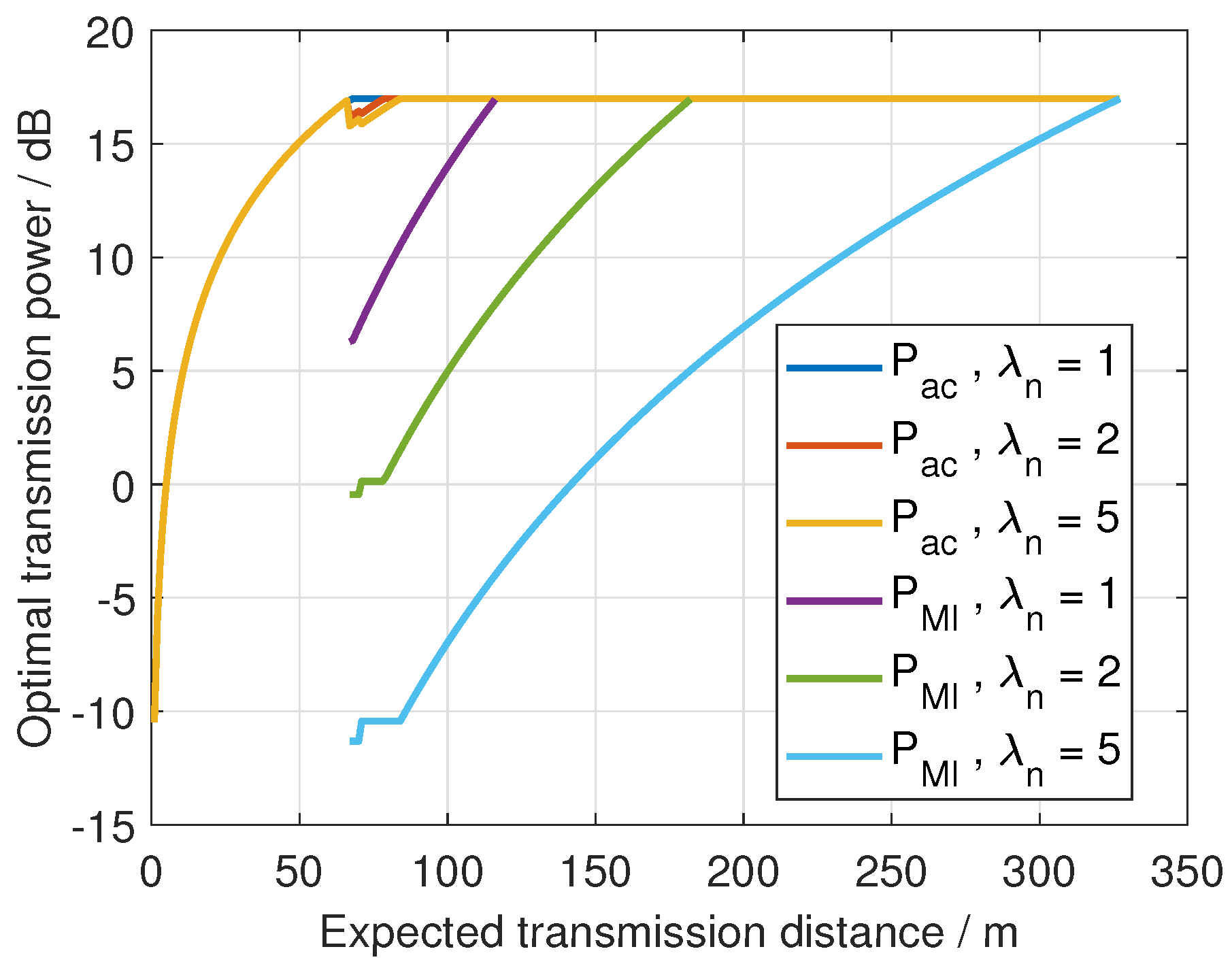
  • A cooperative MIMO size optimization (CMSO) algorithm based on the energy consumption model is proposed, to determine whether to adopt cooperative MIMO and to derive the optimal cooperative MIMO size in theory. It is worth noting that the power allocation for MI and acoustic communication under the maximum transmission power constraint is especially considered.
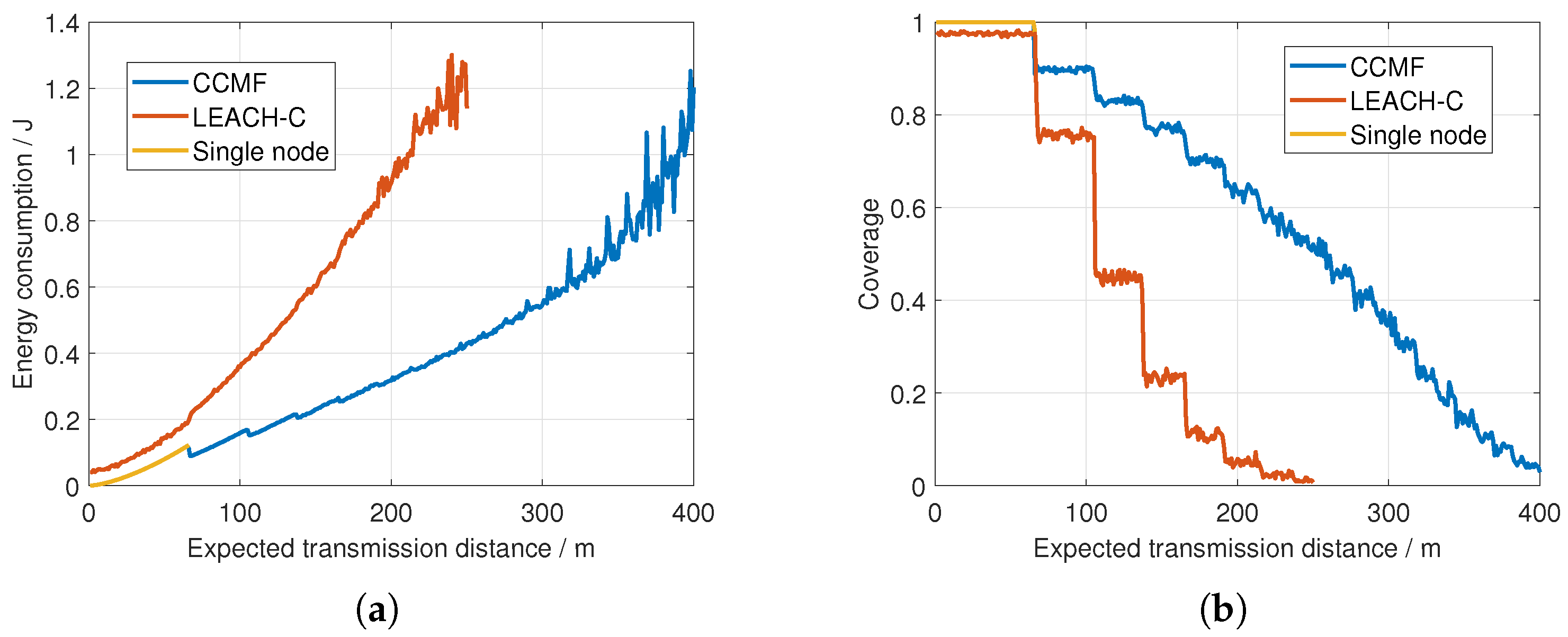
  • In the underwater MI-assisted acoustic cooperative MIMO networks, the expected transmission distance is determined by the distance between the node and the surface BS. Under the requirement of ensuring the network’s connectivity, we propose a competitive cooperative MIMO formation (CCMF) algorithm to select appropriate MN and form cooperative MIMO to prolong network lifetime, in which the optimal cooperative MIMO size determined by the CMSO algorithm is taken as an essential parameter.
The remainder of this article is organized as follows. The scenario is set, and the relevant model is given in Section 2. The optimal cooperative MIMO size can be calculated in Section 3. Section 4 describes our cooperative MIMO formation scheme. The simulation results and performance analysis are discussed in Section 5. Finally, Section 6 concludes the paper.

2. Preliminaries

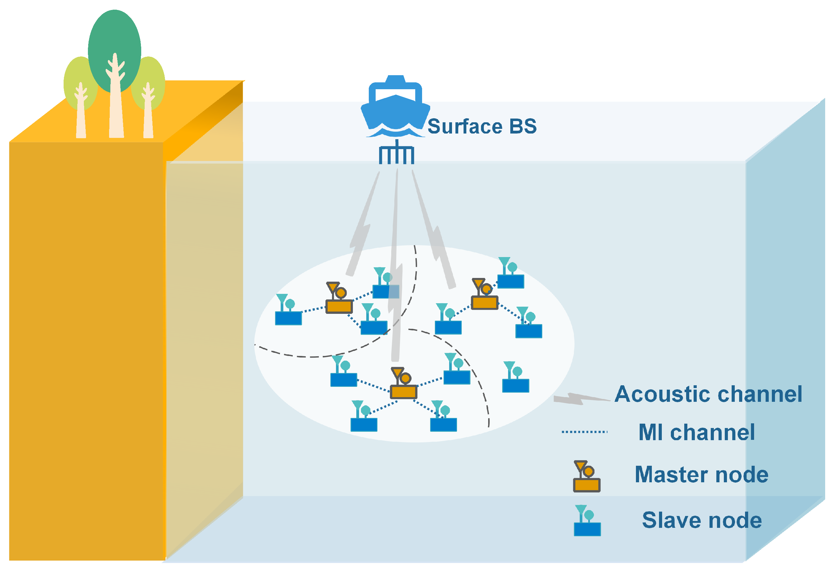
2.1. Scenario and Notation

As shown in Figure 1, we consider one possible underwater sensor network architecture in practical underwater applications. It consists of a surface BS and many underwater sensor nodes. The surface BS is equipped on ships or buoys to aggregate the data from underwater nodes for environment sensing or to release the control information. These sensor nodes are scattered at the bottom of the monitoring waters and are distributed according to a Poisson Point Process with density λ n . Each node is equipped with MI and acoustic modules. They communicate with each other through MI modems, and the underwater nodes cooperatively transmit information to the BS through acoustic modems due to the limited antenna physical size. This paper is based on the following assumptions:
  • The underwater environment is basically stable.
  • Sensors nodes and surface BS are not affected by water flow.
  • Their locations are known with the help of localization techniques.
Because the underwater nodes are closely spaced, the data that the nodes sensed are correlated. Through aggregation, data are compressed due to the exploitation of their spatial correlation, and consequently, much fewer data need to be transmitted from underwater to the remote surface BS [31]. During local communication, underwater nodes need to share the same data and clock to prepare for cooperative transmission in the next step. At the same time, the data need to be compressed and distributed to individual nodes. Therefore, a node is selected as an MN in a cooperative MIMO to coordinate the local synchronization and aggregate data, and other nodes participating in cooperative MIMO act as SNs. The transmission scheme of underwater MI-assisted acoustic cooperative MIMO WSNs is described in detail in Section 2.2.

2.2. Transmission Scheme

To ensure the quality of communication, the operation of the transmission scheme is divided into r o u n d s by the effective communication time [13]. Firstly, a Set-up phase provides the basis for the normal operation of the network, which mainly includes the formation of a cooperative MIMO and synchronization, as seen in Figure 2. It is worth noting that the channel identification is the same as in Figure 1.
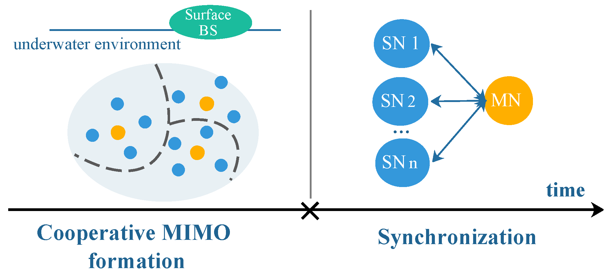
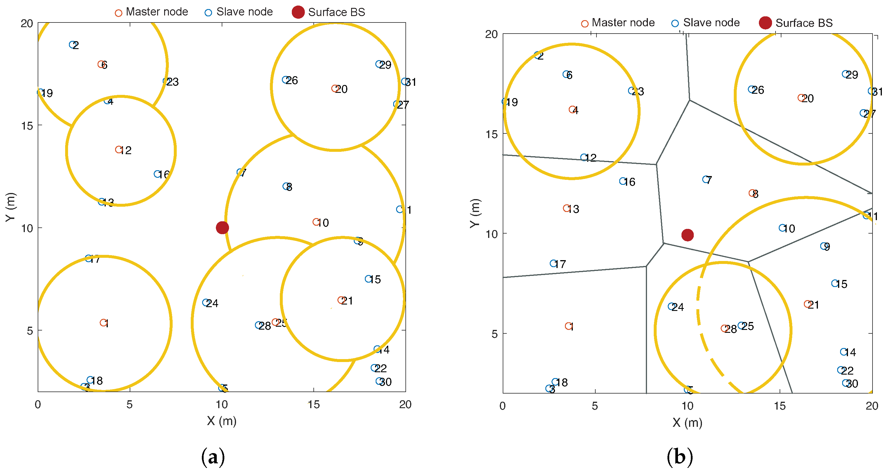
  • Phase 1 (Cooperative MIMO formation) The MN is selected according to the location of the nodes and the number of nodes required to form cooperative MIMO in theory. Then, the remaining nodes are chosen by MN as SN to form a cooperative MIMO. The process is described in detail in Section 4.
  • Phase 2 (Synchronization) The SNs adjust their clocks and frequencies to that of MN by Timing-Sync Protocol for Sensor Networks (TPSN) [36]. For beamforming communications, the CSI of the MN also needs to be delivered to the SNs to compute the beamforming codebook. By considering the optimal phase control, the channel delay can be compensated for by the phase control, and the SNR at the received side can be maximized.
Sequentially, suppose that the node wants to communicate with surface BS in the form of a cooperative MIMO, and this process takes place in the Steady-state phase, as seen in Figure 3.
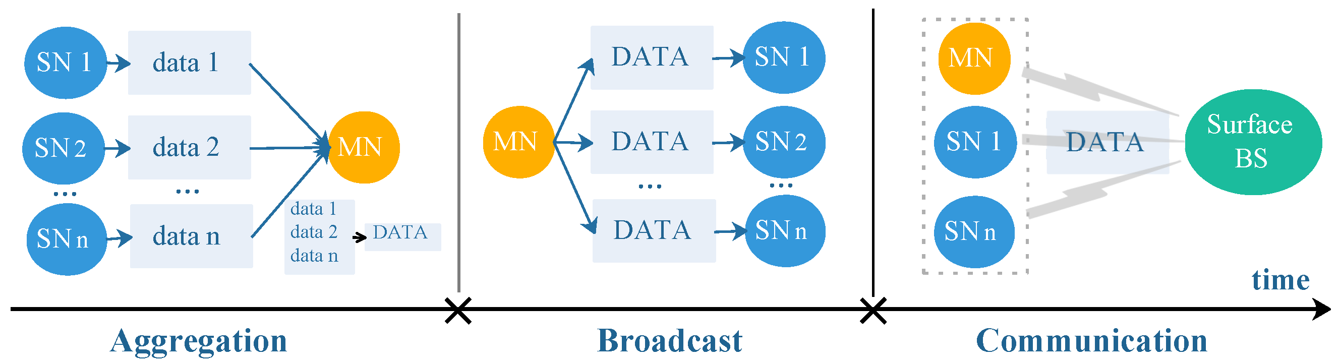
  • Phase 3 (Aggregation). The MN collects the detection information of SNs and compresses the data according to the spatial correlation of the information.
  • Phase 4 (Broadcast). The MN broadcasts the compressed data to their SNs.
  • Phase 5 (Communication). Individual nodes concurrently transmit the compressed data over the acoustic channel to the surface BS using a beamforming scheme.

2.3. Channel Characteristics

There are two types of channels in the underwater MI-assisted acoustic cooperative MIMO WSNs, namely the underwater acoustic channel and MI channel [19].
In underwater MI-assisted acoustic cooperative MIMO WSNs, acoustic communication is adopted for long-haul communication in terms of cooperative MIMO. Attenuation A ( d , f a c ) in an underwater acoustic channel for a signal of frequency f a c over a distance d is given by [37]
A ( d , f a c ) = A 0 d θ a ( f a c ) d ,
where A 0 is the normalizing constant and θ is the spreading factor. The spreading factor θ is between 1 and 2, depending on the depth. The absorption coefficient a ( f a c ) can not be expressed theoretically but is given empirically by Throp’s formula
10 log a ( f a c ) = 0.11 f a c 2 1 + f a c 2 + 44 f a c 2 4100 + f a c 2 + 2.75 × 10 4 f a c 2 + 0.003 ,
where f a c is in kHz and 10 log a ( f a c ) is in dB/km.
Hence, the transmission power model is formulated as
P a c r = P a c t A ( d , f a c ) ,
where P a c r is received power and P a c t is the transmitted power in acoustic communications.
The underwater acoustic ambient noise can be modeled using four sources: turbulence N t , shipping N s , waves N w , and thermal noise N t h . Most of the ambient noise sources can be described by Gaussian statistics and a continuous power spectral density (p.s.d.). The following empirical formulae give the p.s.d. of the four noise components:
10 log N t ( f a c ) = 17 30 log f a c 10 log N s ( f a c ) = 40 + 20 ( s 0.5 ) + 26 log f a c 60 log ( f a c + 0.003 ) 10 log N w ( f a c ) = 50 + 7.5 ω 0.5 + 20 log f a c 40 log ( f a c + 0.4 ) 10 log N t h ( f a c ) = 15 + 20 log f a c .
Turbulence noise influences only the very low frequency region, f a c < 10 Hz. Noise caused by distance shipping is dominant in the frequency region of 10 Hz–100 Hz, and it is modeled through the shipping activity factor s, whose values range between 0 and 1 for low and high activity, respectively. Surface motion, caused by wind-driven waves ( ω is the wind speed in m/s), is the major factor contributing to the noise in the frequency region of 100 Hz–100 kHz (the operating region used by the majority of acoustic systems). Finally, thermal noise becomes dominant for f a c > 100 kHz.
MI is adopted for information aggregation and synchronization between sensor nodes in underwater MI-assisted acoustic cooperative MIMO WSNs. With the mutual inductance M and the optimized load impedance Z L , the transmit power P M I t and the receiving power P M I r can be easily derived based on the basic circuit theory. The path loss of MI communication can be expressed as [38]
P L M I = 10 log P M I r P M I t = 10 log R L 2 ω 2 M 2 R t R L + R r 2 + R t X L + ω L r 2 ,
where ω is the angular frequency of the signal, and R L and X L are the real part and imaginary part of the load impedance Z L , respectively. The mutual inductance M and optimized load impedance Z L can be calculated as:
M = μ π N t N r a t 2 a r 2 2 a t 2 + r 2 3 ,
Z L = R r + ω 2 M 2 R t R t 2 + ω 2 L t 2 + j ω 3 M 2 L t R t 2 + ω 2 L t 2 + ω 2 L t 2 ω L r ,
where μ is permeability, and some related notations about the circuit are summarized in Table 1.
Highly conductive sea water induces a significant eddy current that incurs very high path loss. Therefore, in seawater, the path loss of MI communication also needs to consider the influence of medium loss [39]. The attenuation coefficient α is
α = π f M I μ 0 δ ,
where f M I is the operation frequency, μ 0 is vacuum permeability, and δ represents the medium conductivity that varies with different water types.
Therefore, the path loss caused by the influence of seawater medium P L α (dB) is
P L α = 20 log e α r 8.69 α r .
Finally, the path loss of MI communication in seawater is
P L sea = P L M I + P L α = 10 log P r P t + 8.69 α r .

3. Cooperative MIMO Size Optimization

In this section, we first present an energy model for underwater MI-assisted acoustic cooperative MIMO WSNs in Section 3.1. This model reduces the energy consumption of information transmission by reducing the spatial correlation of monitoring data through data aggregation and considering the power control. We then proposed an optimization framework in Section 3.2. The average energy consumption per node required to send a given number of bits is minimized by optimizing the cooperative MIMO size.

3.1. Energy Model

We now analyze the overall energy consumption of the proposed cooperative scheme. We consider both the transmission energy and the associated circuit energy consumption. According to [31], energy consumption per symbol can be defined as:
E = ( P e l e c + P t ) t + P e l e c · t = ( 2 P e l e c + P t ) t ,
where t is transmission time, P e l e c is the power consumed by the transmitter and receiver circuits, and P t is the transmission power.
Assuming that there are n SNs participating in cooperative MIMO. According to the transmission scheme mentioned in Section 2.2, the average total energy consumption E t o t a l in the Steady-state phase in the network is
E t o t a l = q ( n ) · ( E a + E b ) + E c
where E a , E b and E c are node energy consumption in the Aggregation, Broadcast, and Communication phase, respectively, and q ( n ) is a binary function to determine whether cooperative transmission is carried out.
q ( n ) = 0 n = 0 1 n 1
At the Aggregation phase, MN receives the collected information from SNs in terms of MI communication and compresses the data according to the spatial correlation of the information.
E a = E M N , a + E S N , a + E c o m = n T a ( 2 P e l e c + P M I ) + n L a E c o m p
where, E M N , a and E S N , a are the energy consumption of MN and SN during the Aggregation phase, respectively, and E c o m denotes the energy cost for data compression. T a = L a L a R M I R M I is the time for each SN communication with MN, L a is the data length of each SN, R M I denotes the MI’s data transmission rate, P M I is the MI’s transmission power, and E c o m p denotes the energy cost per bit for data compression.
The MN broadcasts information within a cooperative MIMO by MI communication through the Broadcast phase, and the energy consumed E b is
E b = E M N , b + E S N , b = T b ( P e l e c + P M I + n P e l e c )
where, E M N , b and E S N , b are the energy consumption of MN and SN during the Broadcast phase, respectively. The time of broadcast T b = L b L b R M I R M I ; L b is the total amount of compressed data generated by a set of n SNs after lossless compression and can approximately be calculated by [20]:
L i = L i 1 + 1 1 d i d i c + 1 c + 1 L a , i = 2 , 3 , , n
where L i is the i-th node’s compressed data amount, L 1 = L a , c is a constant and represents the degree of spatial correlation in the data, and d i is the minimum distance between the node i and the other nodes in the cooperative MIMO.
At the Communication phase, the energy consumed of all nodes within the cooperative MIMO when it communicates with surface BS by acoustic can be expressed as
E c = E M N , c + E S N , c = T c ( n + 1 ) ( P e l e c + P a c )
where, E M N , c and E S N , c are the energy consumption of MN and SN during the Communication phase, respectively. The transmission time T c = L b L b R a c R a c related to L b , the acoustic data rate is R a c , and P a c is the acoustic’s transmission power.

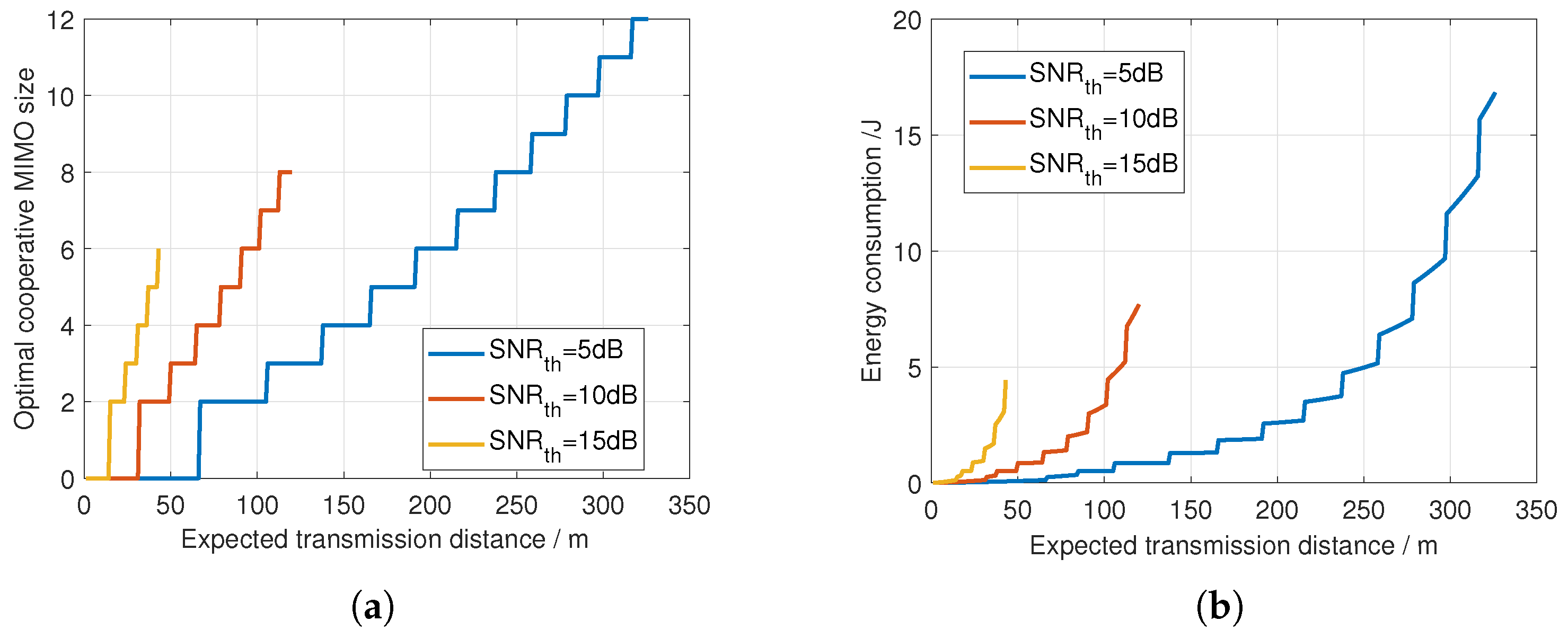
3.2. Cooperative MIMO Size Optimization

To evaluate the connectivity of nodes, we adopt the connectivity definition in [19]. Assume that the distance between two nodes is x, and the maximum transmission distance of the node is R m a x . Then, the connectivity probability of the node is
P c o n n e c t i v i t y = 1 x R max 0 x > R max
where R max is can obtained by
R max = max d : P r P n S N R t h ,
where P r is the received power that is related to the channel state, P n is the power of environment noise, and S N R t h indicates the minimum SNR that the receiving node can receive and recover the transmitted signal sent by the transmitting node. Therefore, two constraints must be satisfied to ensure communication between the underwater node and the surface BS in the underwater MI-assisted acoustic cooperative MIMO WSNs. Firstly, to ensure that MN and SNs within a cooperative MIMO are connected, we have:
P M I r P n S N R t h ,
where P M I r is the power of the received MI signal. To ensure the number of participating nodes n, P M I r is the received power of MN receiving the signal transmitted by the node that is farthest from MN in the cooperative MIMO.
Then the cooperative MIMO connects with the surface BS:
P c M I M O r P n S N R t h ,
where P c M I M O r is the transmitted power of acoustic communication in terms of the cooperative MIMO, and it is related to the number of participating nodes n. Meanwhile, the nodes are distributed according to the homogeneous Poisson point process of intensity λ n ; P c M I M O r can be derived as:
P c M I M O r = k = 0 λ n π r 2 k k ! e λ π r 2 k · P a c t A ( d , f a c ) = λ n π r 2 · P a c t A ( d , f a c ) ,
where r and d are the expected transmission distance of the node and cooperative MIMO, respectively.
Based on the above analysis, the energy consumption of nodes is mainly related to the size of the cooperative MIMO n, and the transmitting power of local P M I t and long-haul communication P a c t . However, in the actual underwater monitoring scenario, the joint optimization of these factors is also affected by the expected transmission distance d and the maximum transmitting power of nodes P m a x .
We now look at the optimization problem for the energy model, which can be expressed as:
min n , P M I t , P a c t E t o t a l s . t . C 1 : n = λ n π r 2 o r 0 C 2 : P M I r σ 2 S N R t h C 3 : λ n π r 2 · P a c t A ( d , f a c ) · σ 2 S N R t h C 4 : P M I t P m a x C 5 : P a c t P m a x ,
where C 1 indicates that the number of cooperative MIMO n is an integer, C 2 makes sure that SNs can connect with the MN, and C 3 makes sure that the cooperative MIMO can achieve the expected transmission distance d. C 4 , and C 5 limit the transmitted power of the node.
We can easily illustrate the tradeoff between the transmission power of acoustic and MI as follows: When the P M I t is large, a large number of nodes can concurrently transmit the data to the surface BS using a beamforming scheme, and a lower transmission power P a c t is needed to satisfy the connection constraint due to the larger cooperative diversity. On the other hand, if P M I t is small, only a few nodes can cooperatively transmit. The limited spatial diversity leads to a larger P a c t . Thus, the MN can control the diversity characteristics of the cooperative scheme via power control [27], and the three variables P M I t , P a c t and n constrain each other in the optimization problem. Moreover, due to the data compression technology that is adopted to minimize data redundancy, the optimization problem (23) contains an iterative function of n, L b [31]. Thus, the minimum E t o t a l can not obtain a closed-form solution. Under the limitation of different expected transmission distances, the CMSO algorithm based on numerical search is proposed, to determine whether to adopt cooperative MIMO and to derive the optimal cooperative MIMO size in theory. It is described in detail in Algorithm 1.
The algorithm starts with the input of the expected transmission distance d, the maximum transmission power of MI, the acoustic communication P m a x , and the SNR threshold S N R t h . Firstly, by substituting P m a x into (20), the maximum transmission distance of MI, r m a x , can be obtained. Due to the MI’s power limit, the SNs can only be selected within r m a x . As the nodes { n j , j = 1 , 2 } are distributed according to the homogeneous Poisson point process of intensity λ n , there is n m a x = λ n π r m a x 2 in theory, and we obtain the interval of cooperative MIMO size [ 1 , n m a x ] (line 1). Then, in each loop, the search range of the cooperative MIMO’s size N ( i ) is determined, and the corresponding acoustic’s transmitting power can be calculated in the interval according to (21). Finally, the search range shown by the Index is determined, and the optimal value is searched in it (line 2–11). When output Index = 1, it can be achieved. Otherwise, it cannot. Due to the number of nodes that form the cooperative MIMO must be an integer, the search step is 1. Meanwhile, the cooperative scheme has no advantage in short transmission-distance scenarios. We compare the energy consumption without cooperative MIMO and E m i n to judge whether to adopt cooperative MIMO (line 12–19). When output Index = 2, the cooperative scheme is cumbersome and rejected.
Algorithm 1 Cooperative MIMO size optimization (CMSO) algorithm.
Input:
d, P m a x , S N R t h .
Output:
n * , P M I * , P a c * , E min , Index.
1: Initialization: Determine the interval N = [ 1 , n m a x ] by P m a x via (20).
2: i = 1.
3: while i n m a x do
4:    With the fixed N ( i ) , obtain the optimal E ( i ) and P MI ( i ) , P ac ( i ) via (23).
5:   if  P ac ( i ) P a c , m a x  then
6:     Index = 1.
7:   else
8:     Index = 0.
9:   end if
10:   i = i + 1.
11: end while
12: if Index = 1 then
13:   Get the optimal E min = m i n ( E ) , and get P M I * , P a c * correspondingly.
14:   Calculate the energy consumption without cooperative MIMO E 0 by n = 0 via (12).
15:   if  E 0 E min , update P M I * , P a c *  then
16:     Index = 2.
17:      E min = E 0 .
18:   end if
19: end if
When the expected transmission distance of a node is determined, Algorithm 1 can determine whether the cooperative transmission is required. This is because when the expected transmission distance is short, the energy consumed by communication between nodes is greater than the energy saved by cooperative MIMO. In addition, when the expected transmission distance is long, due to the limitation of node transmission power, even if cooperative transmission is adopted, long-distance communication cannot be achieved. At this time, other methods, such as relay, need to be considered. Noted that the cooperative MIMO size obtained by Algorithm 1 is a theoretical reference as it is based on the uniform distribution of nodes. In fact, the distribution of nodes could affect the cooperative MIMO’s formation and the setting of the transmitting power. Therefore, the cooperative MIMO is ultimately formed by the CCMF algorithm.

4. Cooperative MIMO Formation Procedure

It can be seen from Section 3 that the expected transmission distance of the different nodes corresponds to different sizes of cooperative MIMOs and the power allocation of balanced local and long-haul communication. Therefore, the underwater nodes forming cooperative MIMOs according to their locations can save node energy consumption and ensure the network’s connectivity. So, in this section, we propose a competitive cooperative MIMO formation algorithm, which considers the MN election to balance the overall energy consumption and apply the theoretical optimal size to the actual network.

4.1. MN Selection

Firstly, the value of node (VoN) has been proposed as a metric to evaluate the potential of nodes as MNs by jointly considering the residual energy of the node and the number of neighbor nodes. A node with higher VoN is more likely to be elected as the MN. Let E n o w , i denote the current energy of node i, and let E 0 be the initial energy of the node; N i denotes the number of the neighbor node, which is defined as within the optimal cooperative MIMO size determined by Algorithm 1, and N is the total number of the nodes. Then, the VoN can be given as:
V i = α E n o w , i E 0 + ( 1 α ) N i N ,
where α is the weighting parameter to measure the tradeoff between the node’s residual energy and the number of neighbor nodes. Due to MN consuming more additional energy at the expense of undertaking tasks such as data aggregation, time synchronization, and so on, it will run out of its energy first and die, resulting in an energy hole in the network, which will significantly reduce the network lifetime. Regarding (24), the node with more residual energy has higher VoN. Similarly, the node with more neighbor nodes can adjust the transmission power of communication according to the distribution of the actual node to reduce energy consumption, so that the VoN value is higher. Such measures will balance the energy consumption between MN and SNs to extend the network’s lifetime.

4.2. Competitive Cooperative MIMO Formation Algorithm

The main idea of the CCMF algorithm is that we first find a list of MN candidates. Then, the nodes run for MN in turn, and the node with enough neighbor nodes can ensure that long-haul communication with surface BS succeeds in the election as MN. The detail of the CCMF algorithm is described in the Algorithm 2. Firstly, the MN candidate list U is derived by sorting VoN according to (24) (line 1 in Algorithm 2). Then, the candidates compete in turn according to U . Based on the above analysis, if the node with a higher VoN is selected as MN, it will balance the energy consumption between MN and SNs to prolong the network’s lifetime. For example, the i-th candidate’s optimal cooperative MIMO range and member number is R i * and n i * , respectively. Within R i * , its available neighbor node set that does not join other cooperative MIMO is C . After that, we judge the competition result (line 4–7 in Algorithm 2). If C = n i * , the candidate i is selected as MN and the cooperative MIMO is determined. Otherwise, the Tire inflation process (Algorithm 3) is adopted to adaptively adjust the cooperative MIMO size. There are two processes in Algorithm 3; the deflation process decreases the size of cooperative MIMO to reduce energy consumption in areas with high node density (line 2–8 in Algorithm 3), and the inflation process increases the size of cooperative MIMO to ensure the connectivity between nodes and surface BS in areas with low node density (line 9–19 in Algorithm 3). It is worth noting that when the number of available neighbor nodes within the maximum communication range of MN candidate U i is less than n i * , that means it can not become an MN, but it still has the potential to be SN. We delete U i from the list U (line 16 in Algorithm 3). When the candidate U i is selected as MN, delete it, and its SNs from the list U and the next round of competition begins (line 8–12 in Algorithm 2).
The CCMS algorithm not only keeps the nodes with high remaining energy to have a priority to be elected as the MN, but also guarantees that the MN is located in the area with high node density and in the center of the cooperative MIMO, which leads to the smaller transmission power. Thus, it balances the total energy consumption and thus prolongs the network lifetime.
Algorithm 2 Competitive cooperative MIMO formation (CCMF) algorithm.
Input:
 Sensor nodes’ location { n j , j = 1 , 2 N } and residue energy
Output:
MN , SN
1: Initialization: Each node runs Algorithm 1 to get its own optimal size n i * , then calculates and sorts its VoN in the descending order as U .
2:  i = 1 .
3: while U do
4:    Set U i as the MN of the cooperative MIMO i, and the nodes within the optimal range of U i are C
5:    if  C n i *  then
6:      Tire inflation process
7:    end if
8:    if  n j C and n j U  then
9:      Delete n j from the list U
10:    end if
11:     M N U i , SN ( i , : ) C
12:     i = i + 1
13: end while
14:  M N , SN
Algorithm 3 Tire inflation process.
Input:
{ n j , j = 1 , 2 N } , C , n i * , R * , ε , R m a x , U
Output:
C , U
1:  R i = R *
2: Deflation process:
3: if C > n i * then
4:    while  C > n i *  do
5:       R i = R i ε
6:      Update the neighbor nodes C using R i
7:    end while
8: end if
9: Inflation process:
10: if C < n i * then
11:    while  C < n i *  do
12:      if  R i < R m a x  then
13:          R i = R i + ε
14:         Update the neighbor nodes C using R i
15:      else
16:         Delete U i from the list U
17:      end if
18:    end while
19: end if

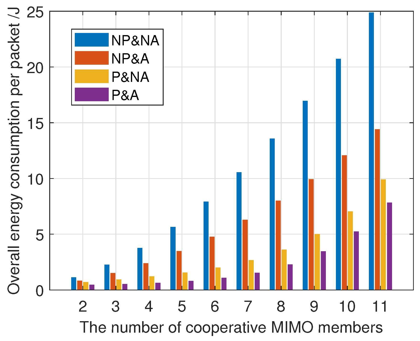
5. Results and Analysis

This part provides simulation results to evaluate the performance of the proposed scheme and algorithms. We first introduce the scenario setup for simulations. Similar to [40], we consider a 3D underwater network with sensors that are initially deployed in a two-dimensional plane at a fixed depth. The distribution of nodes on this plane conforms to a homogeneous Poisson point process with density λ n . The surface BS is placed on the center of the surface. Other detailed parameters are summarized in Table 2 based on several underwater communication channel models and energy consumption models [13,41]. Besides, to equally inspect the influences of all factors, we set the weight parameters to be 0.5, but they can be adjusted in practice.
To show how much energy consumption we have saved in a long-haul communication by combining cooperative MIMO and data aggregation from the previous work, Figure 4 illustrates the overall energy consumption per packet with the different number of cooperative MIMO members under four scenarios: (1) No power control and no data aggregation (NP&NA), (2) No power control but with data aggregation (NP&A), (3) Power control but with no data aggregation (P&NA), and (4) Power control and data aggregation (P&A). The fixed transmission power is 50 W. Note that at the expected transmission distance of 100 m, a single node cannot realize long-haul communication under the constraint of the acoustic’s maximum expected transmission power of 50 W. At the same time, the transmission range of MI communication limits the number of cooperative MIMO nodes under this network setting. In all four scenarios, P&A showed a significant advantage in overall energy consumption per packet for different numbers of cooperative MIMO nodes. In addition, the influence of the cooperative MIMO nodes’ number on energy consumption is also shown. Hence, it is desirable to find an energy-efficient way by choosing the appropriate size, and the CMSO algorithm is proposed.
Figure 5 shows the results of the CMSO algorithm. When the long-haul transmission distance is fixed, the optimal cooperative MIMO size can be derived, which can effectively deal with the energy-efficient problems by combining data aggregation with cooperative communication. The CMSO algorithm determines whether nodes need a cooperative transmission. Take Figure 5a as an example; when the SNR threshold is 5 dB, and the expected transmission distance exceeds 66 m, the advantage of cooperative communication is revealed. A single node can not complete direct communication with BS when the expected transmission distance is more than 66 m. In addition, with the increase in the expected transmission distance, the energy consumption of nodes increases exponentially. Therefore, when the expected transmission distance is too large, the energy problem could be solved through an appropriate routing design, which is our follow-up research direction. At the same time, we compared the influence of different SNR thresholds on the CMSO algorithm. The larger the SNR threshold, the smaller the expected transmission distance that the same node can achieve. In the actual application of USWN, specific requirements can be considered, and the results provide the guideline for the design of underwater MI-assisted acoustic cooperative MIMO WSNs.
The optimal transmission power of MI and the acoustic under different system parameter settings are depicted in Figure 6. The SNR threshold is 5 dB. To clearly show the variation of optimal transmission power with the expected transmission distance, we express it in dB. It can be seen from the figure that when the expected transmission distance has not reached 66 m, the energy consumed by direct communication between a single node and surface BS is less. In this case, the expected transmission distance is increased by continuously increasing the transmission power of the acoustic. The cooperative MIMO can save more energy when the expected transmission distance exceeds 66 m. There is a trade-off between the increased optimal transmission power of MI and the acoustic until the limitation of maximum transmission power is reached. Thus, the growth trend is ladder-shaped. Once the acoustic’s transmission power increases to 50 W, it is necessary to increase the size of the cooperative MIMO to increase the expected transmission distance. Therefore, the transmission power of MI increases rapidly until the threshold is reached, and the maximum transmission power limits the maximum transmission distance of the cooperative MIMO. The calculation shows that number of nodes is same to achieve the minimum energy consumption, despite the different densities. The number of optimal cooperative MIMO nodes is determined when the expected transmission distance is determined. Therefore, the greater the node density, the smaller the optimal transmit power.
The evaluation mechanism is key to measuring the performance of cooperative MIMO formation. This paper evaluates the performance of CCMS formation by using nodes’ energy consumption and network coverage. Meanwhile, the connectivity of nodes is an essential requirement that must be met. The energy consumption can be calculated by (12). Then, the coverage of the network can be formulated as
P c o v e r a g e = i = 1 N P i , c o n n e c t i v i t y N ,
where N is the number of nodes.
Figure 7 shows the average energy consumption and the coverage under 500 Monte Carlo tests attained by the CCMF algorithm, LEACH-C algorithm [22], and single node. Since there is no related cooperative MIMO formation algorithm, the low energy adaptive clustering hierarchy centralized (LEACH-C) algorithm with a similar principle is adopted for comparison. In the clustering algorithm, a cluster is regarded as a cooperative MIMO, and all nodes in the cluster participate in cooperative communication. Compared with Figure 5a, Figure 7 shows that the transmission distance of a single node can only reach 66 m, and the coverage is 0 after that. Meanwhile, the CCMF algorithm proposed by us considers whether cooperative communication is adopted. So that when the transmission distance is short (0∼66 m), the coverage can be guaranteed by the CCMF algorithm while with the same energy consumption as that of a single node. When the expected transmission distance exceeds the maximum transmission distance of a single node, the CCMF algorithm can grow at the expense of the smaller average node energy consumption in exchange for more long-distance communication. With the decrease in network coverage, the energy consumption of nodes fluctuates wildly. It indicates that few nodes can communicate with the surface BS, which has already failed to meet the requirements for the monitoring purposes of UWSNs. Since the LEACH-C algorithm does not consider the constraint of node connectivity in the design process, it is only designed from the perspective of balancing the overall energy consumption of the network. Depending on the cluster’s size setting, the cluster nodes may not connect with the cluster head, due to the limitation of the MI’s transmission distance. So, the network coverage is not 1 in the interval of (0∼66 m). The size of the cooperative MIMO related to the transmission distance affects the network’s coverage, and so the curve of network coverage in Figure 7 appears as ladder-shaped, corresponding to Figure 5a. In a word, Figure 7 shows that the CCMF algorithm has advantages over the LEACH-C algorithm in energy consumption and coverage.
We randomly generated a network in which the nodes are located at a depth of 150 m from the surface. Figure 8 shows the top view of this network with 31 nodes that are uniformly distributed. The surface BS is placed in the center of the surface. Each node competes for MN in turn, according to its residual energy and the distribution of other nodes around it. The nodes are denser, a smaller MI transmit power of the node as MN is needed, and less energy is consumed. However, when the nodes around itself join other cooperative MIMOs, the MN candidate has to increase the radius of the cooperative MIMO to meet the requirement of the number of cooperative MIMO members, so as to realize the communication with surface BS. If the radius exceeds the transmit power limit of MI, the node cannot be selected as MN, but it still has the opportunity to participate in other cooperative MIMOs as SN. Otherwise, the node could be left without a MIMO and be unable to communicate with the surface BS, such as nodes 22, 30, and 31 in Figure 8. Other cluster algorithms do not consider the influence of the number of nodes on clustering. The LEACH-C algorithm takes into account the position of nodes. However, due to the distribution of nodes, the cluster with fewer nodes cannot communicate with surface BS, such as the cluster with nodes 1, 8, and 13 as MN in Figure 8b. Additionally, the network coverage is very low. At the same time, the energy consumption of nodes in some dense regions is very high.
Moreover, in Figure 7a, there are drops in energy consumption with the increase in expected transmission distance. This is because Figure 7 shows the Monte Carlo simulation results of the CCMF algorithm in the actual network scenario. The energy consumption of nodes is affected by node distribution. For example, considering the influence of other cooperative MIMOs, node 10 in Figure 8a must increase the MI transmitting power to ensure the connection with surface BS. Therefore, its energy consumption may exceed the theoretical optimal value. Switching to a larger MIMO will completely change the composition of the network, and the energy consumption of nodes may be reduced, but the corresponding network coverage could be significantly reduced. Figure 7 shows the energy consumption and network coverage versus the expected transmission distance. In network design, a tradeoff between the two parameters needs to be considered according to the actual requirements.
Figure 9 shows the relationship between the number of live nodes and the lifetime. We randomly generated a network in which 18 nodes are located at a distance of 100 m from the surface BS. The initial energy of each node is 40 J. When the remaining energy of the node is less than 20 J, the node is judged to be dead. We adopt the setting because it can intuitively show the influence of different system parameters on the scheme. Figure 5a shows that when the SNR thresholds are 5 dB and 10 dB, the optimal cooperative MIMO numbers are 2 and 6, respectively. Additionally, the expected transmission distance can not reach 100 m with S N R t h = 15 dB . When the requirement for communication quality is relaxed, the SNR threshold is small, and the energy consumed by nodes to transmit the same distance is small, so that the network lifetime is extended. Meanwhile, Figure 9 shows that the nodes almost died at the same time, which indicates that all nodes in the whole network consume very evenly, and this helps to reduce the probability of energy holes and extend the network lifetime. It is worth noting that we tried to compare the CCMS and LEACH-C algorithms, but since the LEACH-C algorithm does not consider the constraints of the expected transmission distance of nodes when forming cooperative MIMOs, the coverage of this network cannot be guaranteed, and there is no comparability. Moreover, the network lifetime can be extended according to the design needs by appropriately setting the SNR threshold, initial node energy, and node death criteria.

6. Conclusions

In this paper, an energy-efficient cooperative MIMO formation mechanism based on data aggregation is proposed for underwater MI-assisted acoustic cooperative MIMO networks. For this purpose, we firstly derive a mathematical energy consumption model. Compared with a traditional MIMO without data aggregation or physical-layer power control, the proposed strategy has demonstrated its performance superiority. It explores the potential of underwater MI-assisted acoustic cooperative MIMO networks in energy saving in long-haul communication. The optimal cooperative MIMO size is obtained based on the derived energy model, which ensures the expected transmission distance. Then, the CCMS algorithm is proposed to form a cooperative MIMO according to the nodes’ geographical location and distribution, so that the nodes’ energy consumption can be reduced under the condition of satisfying the connectivity with the surface BS. The simulation results show that the proposed scheme achieves significant energy savings and prolongs the network lifetime considerably in long-haul communication.
Our proposed scheme can provide a guideline for the design of underwater MI-assisted acoustic cooperative MIMO WSNs. The performance of the network has been evaluated, including energy-efficient, long-range, and high-throughput communication, and other aspects. Therefore, it is suitable for some underwater applications with large ranges, difficult node replacement, and high requirements for underwater communication, such as real-time pollution monitoring, deep sea mining, tsunami early warning, tracking underwater animals, dam structure health monitoring, and mapping the sea bottom. Deploying the nodes at the target area, the underwater MI-assisted acoustic cooperative MIMO network will work according to the transmission mechanism mentioned in Section 2.2, including the Set-up and Steady-state phases. For future work, we plan to research the following two aspects further: (1) It is observed that, as the expected transmission distance increases, simply increasing the size of cooperative MIMO cannot solve the energy problem and guarantee network coverage. The routing strategy should be designed appropriately. (2) Due to the complex underwater environment, if there are damaged underwater sensor nodes, the cooperative MIMO formed by the proposed method cannot connect with surface BS. Therefore, another future work involves designing a cooperative MIMO formation mechanism that can provide fault tolerance without violating the full coverage and connectivity requirements.

Author Contributions

Conceptualization, Q.R. and Y.S.; methodology, Q.R.; validation, Q.R.; investigation, T.W.; resources, B.Z.; writing—original draft preparation, Q.R.; writing—review and editing, T.W. and B.Z.; supervision, Y.S.; project administration, B.Z.; funding acquisition, Y.S. All authors have read and agreed to the published version of the manuscript.

Funding

This research was funded by the Fundamental Research Funds for the Central Universities (2020ZDPY0304).

Data Availability Statement

Not applicable.

Conflicts of Interest

The authors declare no conflict of interest.

References

  1. Darehshoorzadeh, A.; Boukerche, A. Underwater sensor networks: A new challenge for opportunistic routing protocols. IEEE Commun. Mag. 2015, 53, 98–107. [Google Scholar] [CrossRef]
  2. Villa, J.; Aaltonen, J.; Virta, S.; Koskinen, K.T. A Co-Operative Autonomous Offshore System for Target Detection Using Multi-Sensor Technology. Remote Sens. 2020, 12, 4106. [Google Scholar] [CrossRef]
  3. Mezni, H.; Driss, M.; Boulila, W.; Ben Atitallah, S.; Sellami, M.; Alharbi, N. SmartWater: A Service-Oriented and Sensor Cloud-Based Framework for Smart Monitoring of Water Environments. Remote Sens. 2022, 14, 922. [Google Scholar] [CrossRef]
  4. Guo, H.; Sun, Z.; Wang, P. Joint Design of Communication, Wireless Energy Transfer, and Control for Swarm Autonomous Underwater Vehicles. IEEE Trans. Veh. Technol. 2021, 70, 1821–1835. [Google Scholar] [CrossRef]
  5. Stojanovic, M.; Preisig, J. Underwater acoustic communication channels: Propagation models and statistical characterization. IEEE Commun. Mag. 2009, 47, 84–89. [Google Scholar] [CrossRef]
  6. Singer, A.C.; Nelson, J.K.; Kozat, S.S. Signal Processing for Underwater Acoustic Communications. IEEE Commun. Mag. 2009, 47, 90–96. [Google Scholar] [CrossRef]
  7. Coutinho, R.; Boukerche, A.; Vieira, L.; Loureiro, A. On the design of green protocols for underwater sensor networks. IEEE Commun. Mag. 2016, 54, 67–73. [Google Scholar] [CrossRef]
  8. Zhang, J.; Zheng, Y.R. Frequency-Domain Turbo Equalization with Soft Successive Interference Cancellation for Single Carrier MIMO Underwater Acoustic Communications. IEEE Trans. Wirel. Commun. 2011, 10, 2872–2882. [Google Scholar] [CrossRef]
  9. Pailhas, Y.; Petillot, Y.; Brown, K.; Mulgrew, B. Spatially Distributed MIMO Sonar Systems: Principles and Capabilities. IEEE J. Ocean. Eng. 2017, 42, 738–751. [Google Scholar] [CrossRef] [Green Version]
  10. Sklivanitis, G.; Cao, Y.; Batalama, S.N.; Su, W. Distributed MIMO Underwater Systems: Receiver Design and Software-defined Testbed Implementation. In Proceedings of the 2016 IEEE Global Communications Conference (GLOBECOM), Washington, DC, USA, 4–8 December 2016. [Google Scholar]
  11. Kai, T.; Duman, T.M.; Proakis, J.G.; Stojanovic, M. Cooperative MIMO-OFDM communications: Receiver design for Doppler-distorted underwater acoustic channels. In Proceedings of the Signals, Systems & Computers, Pacific Grove, CA, USA, 7–10 November 2010. [Google Scholar]
  12. Brown, D.R.; Poor, H.V. Time-Slotted Round-Trip Carrier Synchronization for Distributed Beamforming. IEEE Trans. Signal Process. 2008, 56, 5630–5643. [Google Scholar] [CrossRef] [Green Version]
  13. Li, Z.; Desai, S.; Soham, S.D.; Wang, P.; Han, J.; Sun, Z. Underwater Cooperative MIMO Communications using Hybrid Acoustic and Magnetic Induction Technique. Comput. Netw. 2020, 173, 487–502. [Google Scholar] [CrossRef] [Green Version]
  14. Guo, H.; Sun, Z.; Wang, P. Multiple Frequency Band Channel Modeling and Analysis for Magnetic Induction Communication in Practical Underwater Environments. IEEE Trans. Veh. Technol. 2017, 66, 6619–6632. [Google Scholar] [CrossRef]
  15. Kisseleff, S.; Akyildiz, I.F.; Gerstacker, W.H. Survey on Advances in Magnetic Induction-Based Wireless Underground Sensor Networks. IEEE Internet Things J. 2017, 5, 4843–4856. [Google Scholar] [CrossRef]
  16. Akyildiz, I.F.; Wang, P.; Sun, Z. Realizing Underwater Communication through Magnetic Induction. IEEE Commun. Mag. 2015, 53, 42–48. [Google Scholar] [CrossRef]
  17. Desai, S.; Sudev, V.D.; Tan, X.; Wang, P.; Sun, Z. Enabling Underwater Acoustic Cooperative MIMO Systems by Metamaterial-Enhanced Magnetic Induction. In Proceedings of the 2019 IEEE Wireless Communications and Networking Conference, Marrakesh, Morocco, 15–18 April 2019. [Google Scholar]
  18. Ren, Q.; Sun, Y.; Li, S.; Zhang, L.; Sun, Z. On Connectivity of Wireless Underwater Sensor Networks Using MI-assisted Acoustic Distributed Beamforming. In Proceedings of the 2019 14th International Conference on Underwater Networks Systems (WUWNET’19), Atlanta, GA, USA, 23–25 October 2019; pp. 370–378. [Google Scholar]
  19. Ren, Q.; Sun, Y.; Huo, Y.; Zhang, L.; Li, S. Connectivity on Underwater MI-Assisted Acoustic Cooperative MIMO Networks. Sensors 2020, 20, 3317. [Google Scholar] [CrossRef]
  20. Pattem, S.; Krishnamachari, B.; Govindan, R. The impact of spatial correlation on routing with compression in wireless sensor networks. In Proceedings of the International Symposium on Information Processing in Sensor Networks, Berkeley, CA, USA, 27 April 2004. [Google Scholar]
  21. Krishnamachari, L.; Estrin, D.; Wicker, S. The Impact of Data Aggregation in Wireless Sensor Networks. In Proceedings of the International Conference on Distributed Computing Systems Workshops, Vienna, Austria, 2–5 July 2002. [Google Scholar]
  22. Heinzelman, W.; Chandrakasan, A.; Balakrishnan, H. An Application-Specific Protocol Architecture for Wireless Microsensor Networks. IEEE Trans. Wirel. Commun. 2002, 1, 660–670. [Google Scholar] [CrossRef] [Green Version]
  23. Yen, H.H.; Lin, C.L. Integrated channel assignment and data aggregation routing problem in wireless sensor networks. IET Commun. 2009, 3, 784–793. [Google Scholar] [CrossRef]
  24. Moh, M.; Kim, E.J.; Moh, T.S. Design and analysis of distributed power scheduling for data aggregation in wireless sensor networks. Int. J. Sens. Netw. 2006, 1, 143–155. [Google Scholar] [CrossRef]
  25. Cui, S.; Goldsmith, A.; Bahai, A. Energy-efficiency of MIMO and Cooperative MIMO Techniques in Sensor Networks. IEEE J. Sel. Areas Commun. 2004, 22, 1089–1098. [Google Scholar] [CrossRef]
  26. Jayaweera, S.K. Virtual MIMO-based Cooperative Communication for Energy-constrained Wireless Sensor Networks. IEEE Trans. Wirel. Commun. 2006, 5, 984–989. [Google Scholar] [CrossRef]
  27. Aminzadeh, R.; Kashefi, F. Energy-Efficient Cooperative Communication in a Clustered Wireless Sensor Network. IEEE Trans. Veh. Technol. 2008, 57, 3618–3628. [Google Scholar]
  28. Zhou, Z.; Zhou, S.; Cui, J.H.; Cui, S. Energy-Efficient Cooperative Communication Based on Power Control and Selective Single-Relay in Wireless Sensor Networks. IEEE Trans. Wirel. Commun. 2008, 7, 3066–3078. [Google Scholar] [CrossRef]
  29. Siam, M.Z.; Krunz, M.; Cui, S.; Muqattash, A. Energy-efficient protocols for wireless networks with adaptive MIMO capabilities. Wirel. Netw. 2010, 16, 199–212. [Google Scholar] [CrossRef] [Green Version]
  30. Rosas, F.; Oberli, C. Effect of the CSI on the energy consumption of MIMO communications. IEEE Trans. Wirel. Commun. 2015, 14, 4156–4169. [Google Scholar] [CrossRef]
  31. Gao, Q.; Zuo, Y.; Zhang, J.; Peng, X. Improving Energy Efficiency in a Wireless Sensor Network by Combining Cooperative MIMO with Data Aggregation. IEEE Trans. Veh. Technol. 2010, 59, 3956–3965. [Google Scholar] [CrossRef] [Green Version]
  32. Zhang, J.; Fei, L.; Gao, Q.; Peng, X.H. Energy-Efficient Multihop Cooperative MISO Transmission with Optimal Hop Distance in Wireless Ad Hoc Networks. IEEE Trans. Wirel. Commun. 2011, 10, 3426–3435. [Google Scholar] [CrossRef] [Green Version]
  33. Guo, S.; Wang, F.; Yang, Y.; Xiao, B. Energy-Efficient Cooperative for Simultaneous Wireless Information and Power Transfer in Clustered Wireless Sensor Networks. IEEE Trans. Commun. 2015, 63, 4405–4417. [Google Scholar] [CrossRef]
  34. Ayatollahi, H.; Tapparello, C.; Heinzelman, W. MAC-LEAP: Multi-antenna, Cross layer, Energy Adaptive Protocol—ScienceDirect. Ad Hoc Netw. 2019, 83, 91–110. [Google Scholar] [CrossRef]
  35. Zhang, Y.; Su, Y.; Shen, X.; Wang, A.; Wang, B.; Liu, Y.; Bai, W. Reinforcement Learning Based Relay Selection for Underwater Acoustic Cooperative Networks. Remote Sens. 2022, 14, 1417. [Google Scholar] [CrossRef]
  36. Ganeriwal, S.; Kumar, R.; Srivastava, M.B. Timing-sync Protocol for Sensor Networks. In Proceedings of the 2003 International Conference on Embedded Networked Sensor Systems, Los Angeles, CA, USA, 5–7 November 2003. [Google Scholar]
  37. Brechovskich, L.M.; Lysanov, J.P. Fundamentals of Ocean Acoustics; Springer: Berlin/Heidelberg, Germany, 1991. [Google Scholar]
  38. Domingo, M.C. Magnetic Induction for Underwater Wireless Communication Networks. IEEE Trans. Antennas Propag. 2012, 60, 2929–2939. [Google Scholar] [CrossRef]
  39. Li, Y.; Wang, S.; Jin, C.; Zhang, Y.; Jiang, T. A Survey of Underwater Magnetic Induction Communications: Fundamental Issues, Recent Advances, and Challenges. IEEE Commun. Surv. Tutor. 2019, 21, 2466–2487. [Google Scholar] [CrossRef]
  40. Ghoreyshi, S.M.; Shahrabi, A.; Boutaleb, T.; Khalily, M. Mobile Data Gathering with Hop-Constrained Clustering in Underwater Sensor Networks. IEEE Access 2019, 7, 21118–21132. [Google Scholar] [CrossRef]
  41. Yu, W.; Chen, Y.; Wan, L.; Zhang, X.; Xu, X. An Energy Optimization Clustering Scheme for Multi-Hop Underwater Acoustic Cooperative Sensor Networks. IEEE Access 2020, 8, 89171–89184. [Google Scholar] [CrossRef]
Figure 1. The system overview of the underwater MI-assisted acoustic cooperative MIMO WSNs.
Remotesensing 14 03641 g001
Figure 2. The process diagram of the Set-up phase.
Remotesensing 14 03641 g002
Figure 3. The process diagram of the Steady-state phase.
Remotesensing 14 03641 g003
Figure 4. The overall energy consumption per packet with different numbers of cooperative MIMO members.
Remotesensing 14 03641 g004
Figure 5. The results of the CMSO algorithm. (a) The optimal number of cooperative MIMO members at different expected transmission distances. (b) The energy consumption per node at different expected transmission distances.
Remotesensing 14 03641 g005
Figure 6. Transmission power of MI and acoustics under different system parameter settings.
Remotesensing 14 03641 g006
Figure 7. Perfomance comparison between CCMF algorithm, LEACH-C algorithm, and other benchmarks. (a) Average energy consumption per node versus expected transmission distance. (b) The coverage versus expected transmission distance.
Remotesensing 14 03641 g007
Figure 8. The examples of the two algorithms. (a) An example of CCMF algorithm. (b) An example of LEACH-C algorithm.
Remotesensing 14 03641 g008
Figure 9. Lifetime versus number of nodes alive.
Remotesensing 14 03641 g009
Table 1. Circuit parameters.
ParameterNotation
a t The radius of the transmitting coil
a r The radius of the receiving coil
N t The number of turns of the transmitting coil
N r The number of turns of the receiving coil
L t The self inductance of the transmitting coil
L r The self inductance of the receiving coil
R t The resistance of the transmitting coil
R r The resistance of the receiving coil
Z t The impedance of the transmitting coil
Z r The impedance of the receiving coil
Z r t The reflected impedance of the receiver on the transmitter
Z t r The reflected impedance of the transmitter on the receiver
Z L The load impedance
Table 2. Simulation parameters.
ParameterValue
Maximal transmission power of MI P M I , m a x [41]50 W
Maximal transmission power of acoustic P a c , m a x [41]50 W
Circuits’ power consumed P e l e c [41]0.158 W
Frequency of MI f M I [13]1 MHz
Data transmission rate of MI R M I [13,31]40 kbit/s
Data transmission rate of acoustic R a c [13,31]20 kbit/s
Frequency of ac f a c [13]10 kHz
Circuits’ size r c [13]0.1 m
Total noise for MI [13] 9.81 × 10 3 mW
Shipping activity factor s [35]0.5
Wind speed ω [35]0 m/s
Packet lengths D50 bits
Publisher’s Note: MDPI stays neutral with regard to jurisdictional claims in published maps and institutional affiliations.

