
Evolutionary Computational Intelligence-Based Multi-Objective Sensor Management for Multi-Target Tracking

Abstract
:
1. Introduction
2. Background
2.1. Labeled RFS
2.2. Labeled Multi-Bernoulli Filter
3. Method
3.1. Objective Functions Proposal
3.2. Evolutionary Multi-Objective Optimization
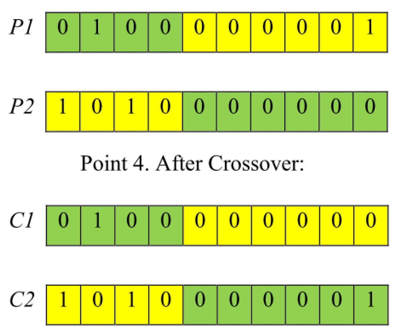
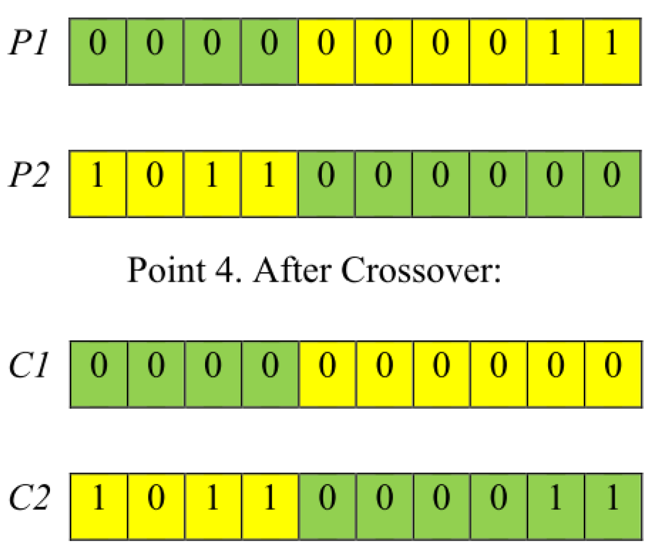
| Algorithm 1 Binary constrained crossover. |
|
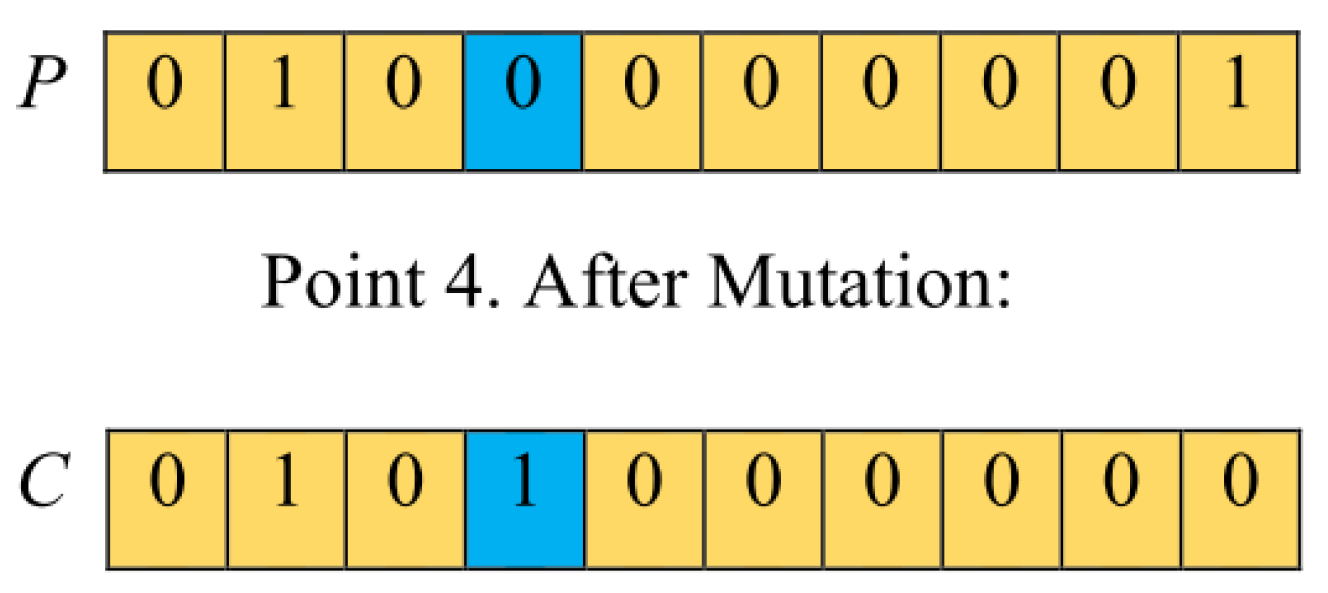
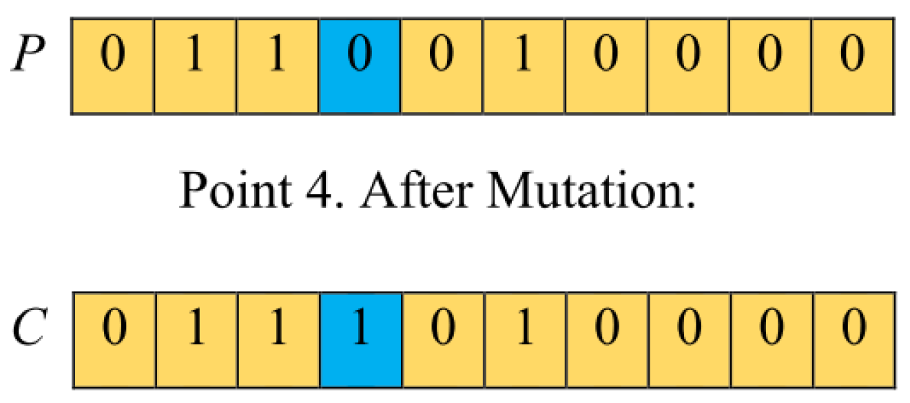
| Algorithm 2 Binary constrained mutation. |
|
- i:
- Normalizethe objective function values of Pareto solutions, as follows
- ii:
- Find the reference network points
- iii:
- Estimate the difference between and
- iv:
- Find the value of GRC for each optimal solution:where and .
- v:
- Find the largest , and the corresponding solution is recommended.
3.3. Multi-Sensor Fusion
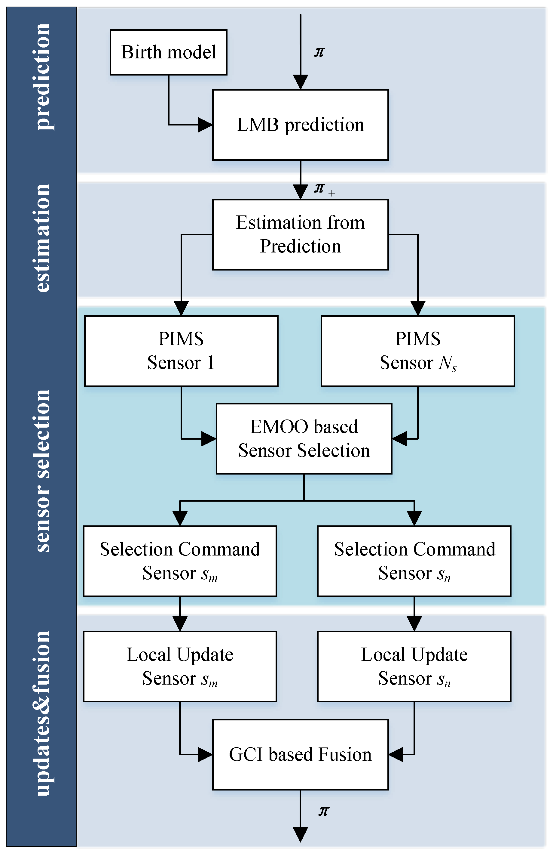
3.4. Step-by-Step Implementation
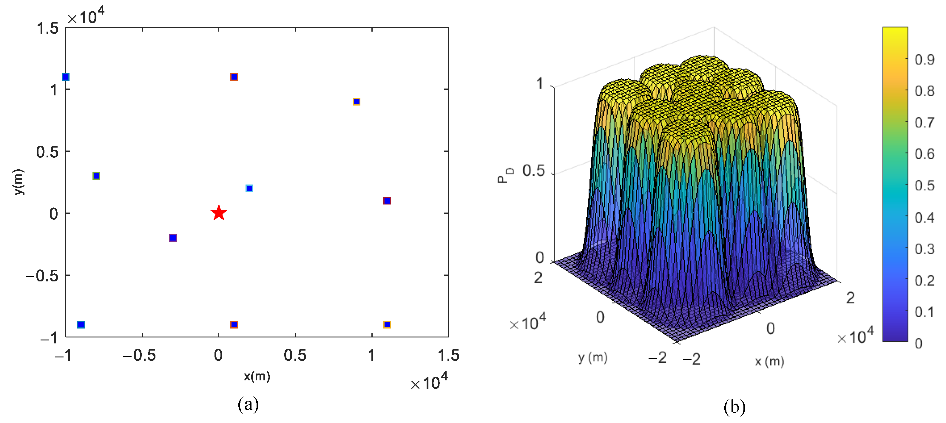
- Sensor model parameters: the number of candidate sensors and their positions , detection probabilities , and clutter intensities with ;
- Birth model parameters: ;
- Likelihood and transition density ;
- Survival probability function: ;
- Constraints on the number of selected sensors: and .
| Algorithm 3 Step-by-step pseudocode for the proposed approach with LMB filtering, sensor selection, and fusion. |
| INPUTS: → LMB distribution from previous time step OUTPUTS: → The posterior parameters to be propagated to the next time step → Estimated multi-target states at the current time
|
| Algorithm 4 Step-by-step pseudocode for the EMOO-based sensor selection. |
| INPUTS: → The predicted LMB distribution → PIMS from each sensor → The population size → The maximum number G of generations OUTPUTS: → The sensors selected at current time
|
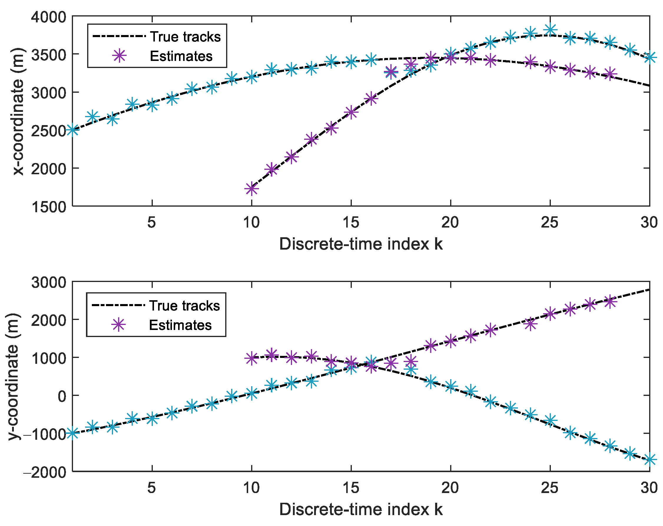
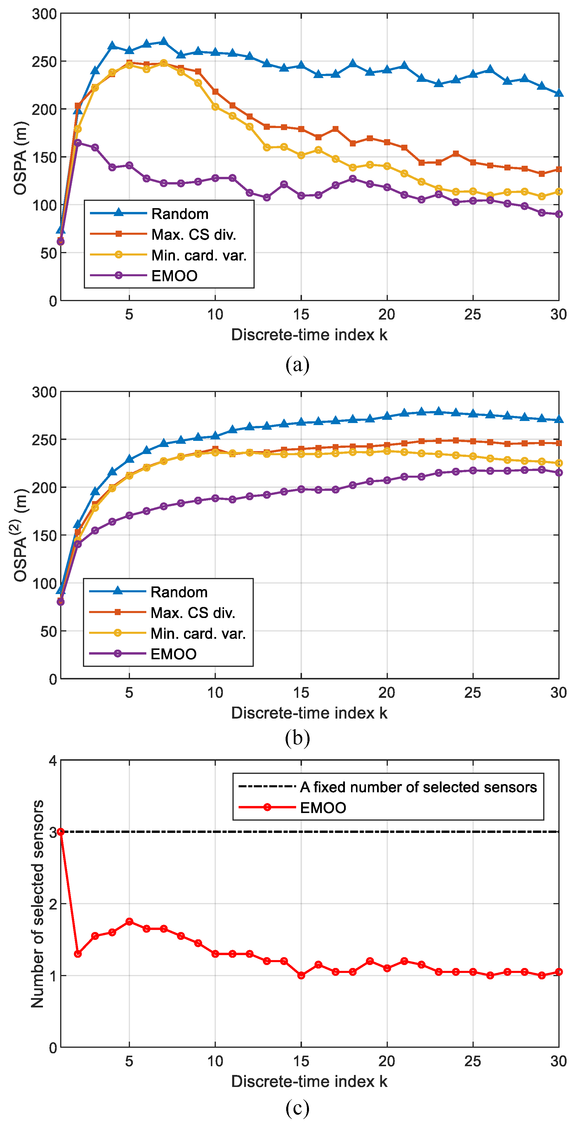
4. Experiments
4.1. Scenario 1
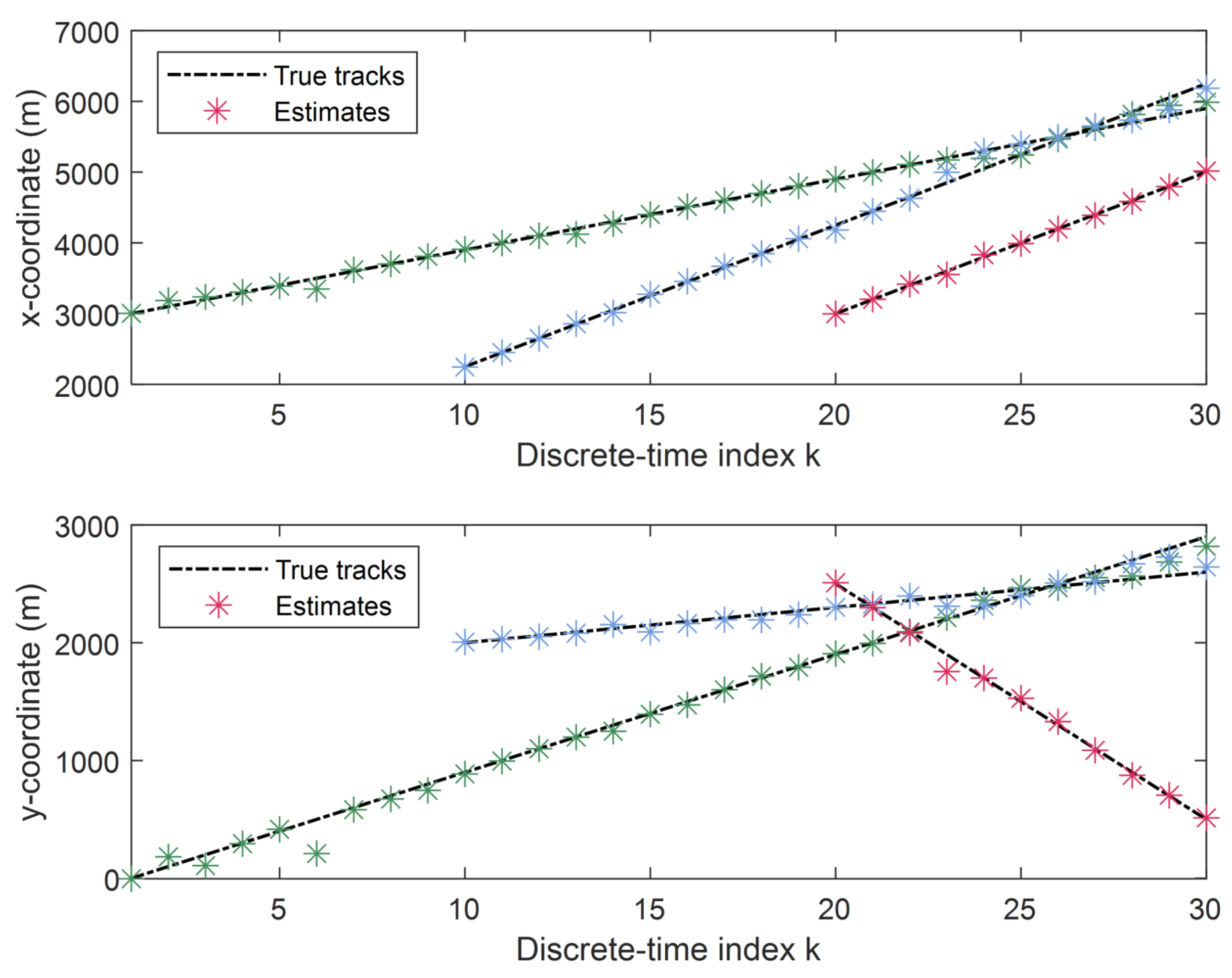
4.2. Scenario 2
5. Discussion
6. Conclusions
Author Contributions
Funding
Data Availability Statement
Conflicts of Interest
References
- Gao, J.; Zhang, Q.; Sun, H.; Wang, W. A Multi-Sensor Interacted Vehicle-Tracking Algorithm with Time-Varying Observation Error. Remote Sens. 2022, 14, 2176. [Google Scholar] [CrossRef]
- Memon, S.A.; Ullah, I.; Khan, U.; Song, T.L. Smoothing Linear Multi-Target Tracking Using Integrated Track Splitting Filter. Remote Sens. 2022, 14, 1289. [Google Scholar] [CrossRef]
- Mallick, M.; Krishnamurthy, V.; Vo, B.N. Integrated Tracking, Classification, and Sensor Management: Theory and Applications; Wiley Press: Hoboken, NJ, USA, 2012. [Google Scholar]
- Bar-Shalom, Y.; Willett, P.; Tian, X. Tracking and Data Fusion: A Handbook of Algorithms; YBS Publishing: Storrs, CT, USA, 2011. [Google Scholar]
- Mahler, R. Global Posterior Densities for Sensor Management. In Acquisition, Tracking, and Pointing XII; SPIE: Bellingham, WA, USA, 1998; pp. 252–263. [Google Scholar]
- Reid, D. An Algorithm for Tracking Multiple Targets. IEEE Trans. Autom. Control 1979, 24, 843–854. [Google Scholar] [CrossRef]
- Kurien, T. Issues in The Design of Practical Multitarget Tracking Algorithms. In Multitarget-Multisensor Tracking: Advanced Applications; Bar-Shalom, Y., Ed.; Artech House: Norwood, MA, USA, 1990; pp. 43–83. [Google Scholar]
- Fortmann, T.; Bar-Shalom, Y.; Scheffe, M. Sonar Tracking of Multiple Targets Using Joint Probabilistic Data Association. IEEE J. Ocean. Eng. 2003, 8, 173–184. [Google Scholar] [CrossRef] [Green Version]
- Mahler, R. Statistical Multisource-Multitarget Information Fusion; Artech House: Norwood, MA, USA, 2007. [Google Scholar]
- Mahler, R. Advances in Statistical Multisource-Multitarget Information Fusion; Artech House: Norwood, MA, USA, 2014. [Google Scholar]
- Mahler, R. Multitarget Bayes Filtering via First-order Multitarget Moments. IEEE Trans. Aerosp. Electron. Syst. 2003, 39, 1152–1178. [Google Scholar] [CrossRef]
- Mahler, R. PHD Filters of Higher Order in Target Number. IEEE Trans. Aerosp. Electron. Syst. 2007, 43, 1523–1543. [Google Scholar] [CrossRef]
- Vo, B.T.; Vo, B.N.; Cantoni, A. The Cardinality Balanced Multi-Target Multi-Bernoulli Filter and Its Implementations. IEEE Trans. Signal Process. 2009, 57, 409–423. [Google Scholar]
- Vo, B.T.; Vo, B.N. Labeled Random Finite Sets and Multi-Object Conjugate Priors. IEEE Trans. Signal Process. 2013, 61, 3460–3475. [Google Scholar] [CrossRef]
- Vo, B.T.; Vo, B.N. A Random Finite Set Conjugate Prior and Application to Multi-target Tracking. In Proceedings of the 2011 7th International Conference on Intelligent Sensors, Sensor Networks and Information Processing, Adelaide, SA, Australia, 6–9 December 2011; pp. 431–436. [Google Scholar]
- Vo, B.N.; Vo, B.T.; Phung, D. Labeled Random Finite Sets and the Bayes Multi-Target Tracking Filter. IEEE Trans. Signal Process. 2014, 62, 6554–6567. [Google Scholar] [CrossRef] [Green Version]
- Reuter, S.; Vo, B.T.; Vo, B.N.; Dietmayer, K. The Labeled Multi-Bernoulli Filter. IEEE Trans. Signal Process. 2014, 62, 3246–3260. [Google Scholar]
- Hero, A.O.; Kreucher, C.M.; Blatt, D. Information Theoretic Approaches to Sensor Management. In Foundations and Applications of Sensor Management; Hero, A.O., Castanon, D., Cochran, D., Kastella, K., Eds.; Springer: Berlin/Heidelberg, Germany, 2008; Chapter 3; pp. 33–57. [Google Scholar]
- Ristic, B.; Vo, B. Sensor Control for Multi-object State-space Estimation Using Random Finite Sets. Automatica 2010, 46, 1812–1818. [Google Scholar] [CrossRef]
- Cai, H.; Gehly, S.; Yang, Y.; Hoseinnezhad, R.; Norman, R.; Zhang, K. Multisensor Tasking Using Analytical Renyi Divergence in Labeled Multi-Bernoulli Filtering. J. Guid. Control Dyn. 2019, 42, 2078–2085. [Google Scholar] [CrossRef]
- Hoang, H.G.; Vo, B.N.; Vo, B.T.; Mahler, R. The Cauchy-Schwarz Divergence for Poisson Point Processes. IEEE Trans. Inf. Theory 2015, 61, 4475–4485. [Google Scholar] [CrossRef] [Green Version]
- Beard, M.; Vo, B.T.; Vo, B.N.; Arulampalam, S. Void Probabilities and Cauchy-Schwarz Divergence for Generalized Labeled Multi-Bernoulli Models. IEEE Trans. Signal Process. 2017, 65, 5047–5061. [Google Scholar] [CrossRef] [Green Version]
- Gostar, A.K.; Hoseinnezhad, R.; Bab-Hadiashar, A.; Liu, W. Sensor-Management for Multitarget Filters via Minimization of Posterior Dispersion. IEEE Trans. Aerosp. Electron. Syst. 2017, 53, 2877–2884. [Google Scholar] [CrossRef]
- Nguyen, H.V.; Rezatofighi, H.; Vo, B.N.; Ranasinghe, D.C. Online UAV Path Planning for Joint Detection and Tracking of Multiple Radio-Tagged Objects. IEEE Trans. Signal Process. 2019, 67, 5365–5379. [Google Scholar] [CrossRef] [Green Version]
- Jiang, M.; Yi, W.; Kong, L. Multi-sensor Control for Multi-target Tracking Using Cauchy-Schwarz Divergence. In Proceedings of the 2016 19th International Conference on Information Fusion (FUSION), Heidelberg, Germany, 5–8 July 2016; pp. 2059–2066. [Google Scholar]
- Hoang, H.G.; Vo, B.T. Sensor Management for Multi-target Tracking via Multi-Bernoulli Filtering. Automatica 2014, 50, 1135–1142. [Google Scholar] [CrossRef] [Green Version]
- Gostar, A.K.; Hoseinnezhad, R.; Bab-Hadiashar, A. Multi-Bernoulli Sensor Control via Minimization of Expected Estimation Errors. IEEE Trans. Aerosp. Electron. Syst. 2015, 51, 1762–1773. [Google Scholar] [CrossRef] [Green Version]
- Panicker, S.; Gostar, A.K.; Bab-Haidashar, A.; Hoseinnezhad, R. Sensor Control for Selective Object Tracking Using Labeled Multi-Bernoulli Filter. In Proceedings of the 2018 21st International Conference on Information Fusion (FUSION), Cambridge, UK, 10–13 July 2018; pp. 2218–2224. [Google Scholar]
- Panicker, S.; Gostar, A.K.; Bab-Hadiashar, A.; Hoseinnezhad, R. Tracking of Targets of Interest Using Labeled Multi-Bernoulli Filter with Multi-Sensor Control. Signal Process. 2020, 171, 107451. [Google Scholar] [CrossRef]
- Nguyen, H.V.; Rezatofighi, H.; Vo, B.N.; Ranasinghe, D. Multi-Objective Multi-Agent Planning for Jointly Discovering and Tracking Mobile Object. In Proceedings of the AAAI Conference on Artificial Intelligence, New York, NY, USA, 7–12 February 2020; pp. 7227–7235. [Google Scholar]
- Zhu, Y.; Wang, J.; Liang, S. Multi-Objective Optimization Based Multi-Bernoulli Sensor Selection for Multi-Target Tracking. Sensors 2019, 19, 980. [Google Scholar] [CrossRef] [Green Version]
- Ma, L.; Xue, K.; Wang, P. Multitarget Tracking with Spatial Nonmaximum Suppressed Sensor Selection. Math. Probl. Eng. 2015, 2015, 148081. [Google Scholar] [CrossRef]
- Ma, L.; Xue, K.; Wang, P. Distributed Multiagent Control Approach for Multitarget Tracking. Math. Probl. Eng. 2015, 2015, 903682. [Google Scholar] [CrossRef] [Green Version]
- Wang, X.; Hoseinnezhad, R.; Gostar, A.K.; Rathnayake, T.; Xu, B.; Bab-Hadiashar, A. Multi-sensor Control for Multi-object Bayes Filters. Signal Process. 2018, 142, 260–270. [Google Scholar] [CrossRef] [Green Version]
- Cao, N.; Choi, S.; Masazade, E.; Varshney, P.K. Sensor Selection for Target Tracking in Wireless Sensor Networks with Uncertainty. IEEE Trans. Signal Process. 2016, 64, 5191–5204. [Google Scholar] [CrossRef] [Green Version]
- Fantacci, C.; Vo, B.N.; Vo, B.T.; Battistelli, G.; Chisci, L. Consensus Labeled Random Finite Set Filtering for Distributed Multi-Object Tracking. arXiv 2015, arXiv:1501.01579. [Google Scholar]
- Mahler, R. Multitarget Sensor Management of Dispersed Mobile Sensors. In Theory and Algorithms for Cooperative Systems; Grundel, D., Murphey, R., Pardalos, P.M., Eds.; World Scientific: Singapore, 2004; pp. 239–310. [Google Scholar]
- Li, H.; Gong, M.; Wang, C.; Miao, Q. Pareto Self-Paced Learning Based on Differential Evolution. IEEE Trans. Cybern. 2021, 51, 4187–4200. [Google Scholar] [CrossRef]
- Gong, M.; Li, H.; Luo, E.; Liu, J.; Liu, J. A Multiobjective Cooperative Coevolutionary Algorithm for Hyperspectral Sparse Unmixing. IEEE Trans. Evol. Comput. 2017, 21, 234–248. [Google Scholar] [CrossRef]
- Gong, M.; Li, H.; Meng, D.; Miao, Q.; Liu, J. Decomposition-Based Evolutionary Multiobjective Optimization to Self-Paced Learning. IEEE Trans. Evol. Comput. 2019, 23, 288–302. [Google Scholar] [CrossRef]
- Ma, L.; Gong, M.; Yan, J.; Yuan, F. A Decomposition-based Multiobjective Evolutionary Algorithm for Analyzing Network Structural Balance. Inf. Sci. 2017, 378, 144–160. [Google Scholar] [CrossRef]
- Ngatchou, P.; Zarei, A.; El-Sharkawi, A. Pareto Multi-Objective Optimization. In Proceedings of the 2005 13th International Conference on, Intelligent Systems Application to Power Systems, Arlington, VA, USA, 6–10 November 2005; pp. 84–91. [Google Scholar]
- Deng, J.L. Control Problems of Grey Systems. Syst. Control Lett. 1982, 1, 288–294. [Google Scholar]
- Ristic, B.; Arulampalam, S.; Gordon, N. Beyond the Kalman Filter-Particle Filters for Tracking Applications; Artech House: Norwood, MA, USA, 2004. [Google Scholar]
- Willis, N.J.; Griffiths, H.D. Advances in Bistatic Radar; SciTech Publishing Inc.: Raleigh, NC, USA, 2007. [Google Scholar]
- Ristic, B.; Farina, A. Target Tracking via Multi-static Doppler Shifts. IET Radar Sonar Navig. 2013, 7, 508–516. [Google Scholar]
- Mahafza, B. Radar Systems Analysis and Design Using MATLAB, 3rd ed.; Chapman and Hall/CRC Press: Boca Raton, FL, USA, 2013. [Google Scholar]
- Schuhmacher, D.; Vo, B.T.; Vo, B.N. A Consistent Metric for Performance Evaluation of Multi-Object Filters. IEEE Trans. Signal Process. 2008, 56, 3447–3457. [Google Scholar] [CrossRef] [Green Version]
- Beard, M.; Vo, B.T.; Vo, B.N. A Solution for Large-Scale Multi-Object Tracking. IEEE Trans. Signal Process. 2020, 68, 2754–2769. [Google Scholar] [CrossRef] [Green Version]
- Beard, M.; Vo, B.T.; Vo, B.N. Performance Evaluation for Large-Scale Multi-Target Tracking Algorithms. In Proceedings of the 2018 21st International Conference on Information Fusion (FUSION), Cambridge, UK, 10–13 July 2018; pp. 1–5. [Google Scholar]


Publisher’s Note: MDPI stays neutral with regard to jurisdictional claims in published maps and institutional affiliations. |
© 2022 by the authors. Licensee MDPI, Basel, Switzerland. This article is an open access article distributed under the terms and conditions of the Creative Commons Attribution (CC BY) license (https://creativecommons.org/licenses/by/4.0/).
Share and Cite
Liang, S.; Zhu, Y.; Li, H.; Yan, J. Evolutionary Computational Intelligence-Based Multi-Objective Sensor Management for Multi-Target Tracking. Remote Sens. 2022, 14, 3624. https://doi.org/10.3390/rs14153624
Liang S, Zhu Y, Li H, Yan J. Evolutionary Computational Intelligence-Based Multi-Objective Sensor Management for Multi-Target Tracking. Remote Sensing. 2022; 14(15):3624. https://doi.org/10.3390/rs14153624
Chicago/Turabian StyleLiang, Shuang, Yun Zhu, Hao Li, and Junkun Yan. 2022. "Evolutionary Computational Intelligence-Based Multi-Objective Sensor Management for Multi-Target Tracking" Remote Sensing 14, no. 15: 3624. https://doi.org/10.3390/rs14153624