Technical Note

Machine Learning to Identify Three Types of Oceanic Fronts Associated with the Changjiang Diluted Water in the East China Sea between 1997 and 2021

1
Department of Oceanography, Pusan National University, Busan 46241, Korea
2
BK21 School of Earth Environmental System, Pusan National University, Busan 46241, Korea
*
Author to whom correspondence should be addressed.
Remote Sens. 2022, 14(15), 3574; https://doi.org/10.3390/rs14153574
Submission received: 26 May 2022 / Revised: 22 July 2022 / Accepted: 22 July 2022 / Published: 25 July 2022
(This article belongs to the Topic Advances in Environmental Remote Sensing)

Abstract

:
Long-term sea surface salinity (SSS) in the East China Sea (ECS) was estimated based on Ocean Color Climate Change Initiative (OC-CCI) data using machine learning during the summer season (June to September) from 1997 to 2021. Changjiang diluted water (CDW) in the ECS propagates northeastward and forms longitudinally-oriented ocean fronts. To determine the CDW’s distribution, three fronts were investigated: (1) a CDW front based on chlorophyll-a concentration (Chl), SSS, and sea surface temperature (SST); (2) a CDW front based on sea surface density (SSD); and (3) a CDW front for nutrient distribution. The Chl fronts matched well with the SSS fronts, suggesting that Chl variation in the ECS is highly correlated with the CDW. Furthermore, the SSD fronts spatially matched well with nitrogen concentration. Sea level anomaly (SLA) variation with SSD was also detected, indicating that CDW had sufficiently large effects on SLA so that they may be detectable by altimeter measurements. This result suggests that the influence of steric height changes and the inflow from rivers are significant in the ECS. Additionally, the continuous long-term SSD developed in this study enables researchers to detect the CDW front and its influence on the ECS marine environment.

1. Introduction

Because Changjiang diluted water (CDW) includes freshwater, nutrients, and sediments, understanding the variations in CDW systems is crucial for analyzing material transport and biogeochemical processes in the East China Sea (ECS) [1,2,3]. CDW detection has been attemptI confirmed using satellite measurements of sea surface salinity (SSS), chlorophyll-a concentration (Chl), and turbidity; however, studies on long-term SSS distribution patterns are scarce, possibly because of limitations in continuous measurements [2,4].
Several recent studies have demonstrated the potential of ocean color satellite remote sensing for estimating the SSS in the ECS [2,5,6]. This is because CDW contains colored dissolved solids or pollutant matter that reflects light at specific wavelengths, such as colored dissolved organic matter (CDOM) and terrestrial particles; the optical feature of CDW is indirectly related to SSS. Based on this principle, Kim et al. [6] estimated the SSS using Geostationary Ocean Color Imager (GOCI, 500 m resolution) data from 2015 to 2020. The application of the same approach also detected SSS variation due to river discharge near the estuaries of the mid-Atlantic [7] and Gulf of Mexico [8], suggesting that SSS variation may be monitored globally using ocean color satellite sensors.
Kim et al. [4] defined CDW based on statistical analysis with the K-means clustering technique using Sea-viewing Wide Field-of-view Sensor (SeaWiFS) Chl in the summer in the ECS from 1998 to 2007. The study results revealed the interannual variation in the CDW indicated by the high satellite Chl and correlated it with the interannual variation in the Changjiang summer freshwater discharge. Bai et al. [2] analyzed summertime CDW variations from 1998 to 2010 using the remote sensing reflectance (Rrs) of SeaWiFS. This study identified three types of plume shapes: (1) the commonly known northeastward transportation, (2) a case in which most of the CDW is to the north of Jeju Island, and (3) a rare case in which the CDW front is transported southeastward. The plume shapes were related to discharge, wind speed in the 45° and 60° directions, and typhoons. Although these studies analyzed the CDW distribution over 10 years, they mainly focused on the variation in CDW distribution and did not investigate the impact of CDW fronts on the biogeochemical environment in the ECS.
Because the Changjiang River is one of the primary ECS nutrient sources, plume water is rich in nutrients compared with that of ambient seawater [9,10,11]. In particular, dissolved inorganic nitrogen (DIN) and phosphate (DIP) fluxes have increased owing to the widespread use of chemical fertilizers in the Changjiang River basin [12]. Kwon et al. [13] analyzed DIN and DIP concentrations from the Changjiang River Estuary to the Korean Strait. The concentrations of DIN and DIP decreased sharply from the river mouth and were depleted within 200 km, and subsequently maintained approximately 0.28 μM L−1 and 0.07 μ M L−1, respectively, until 800 km. However, the analysis of DIN and DIP concentrations depending on CDW extension was conducted in previous studies because of the limitation of the spatiotemporal coverage of shipboard surveys. Therefore, satellite-based CDW monitoring and analysis with in situ chemical measurements are required.
Therefore, the objective of this study was to estimate the long-term SSS distribution using 25 years of satellite observations and to determine the biogeochemical influence of CDW. Because oceanic fronts offer habitats for marine biology, detecting the principal front is an important task. This study presents the differences in the location of the SSS, Chl, sea surface temperature (SST), and sea surface density (SSD) fronts. In addition, the nitrogen and phosphate distributions were compared to the CDW front locations.

2. Materials and Methods

2.1. Materials

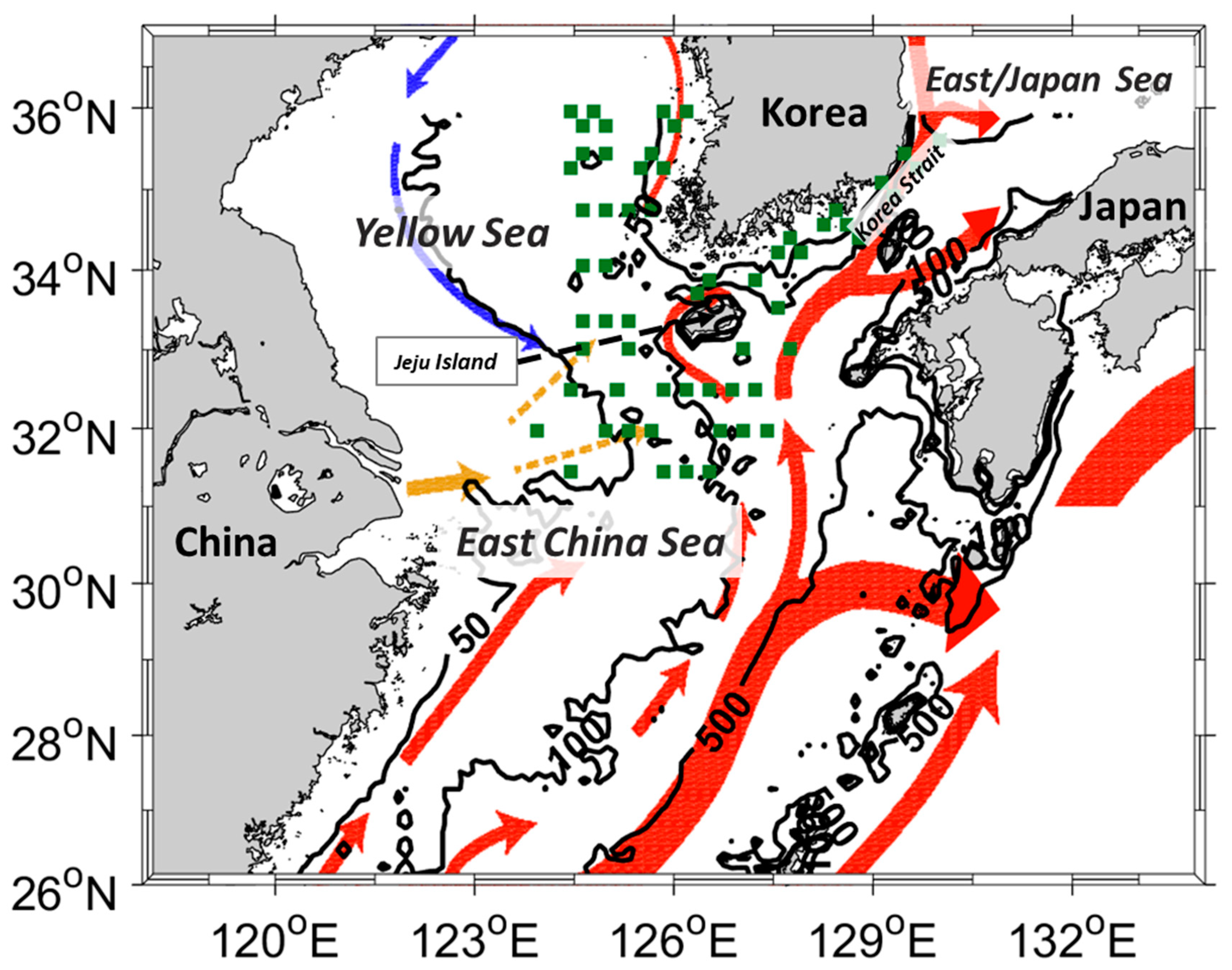
2.1.1. Satellite Data

To estimate the long-term SSS in the ECS, Rrs measurements derived from the Ocean Color Climate Change Initiative (OC-CCI) version 5.0 were used [14]. The OC-CCI products were developed by merging observations from the SeaWiFS, moderate resolution imaging spectroradiometer onboard the Aqua Earth Observing System (MODIS-Aqua), and Medium Resolution Imaging Spectrometer (MERIS). The products were constructed based on SeaWiFS datasets, and the atmospherically corrected Rrs values of MODIS and MERIS data were shifted to the nearest SeaWiFS bands (412, 443, 490, 510, 560, and 665 nm) based on a bio-optical model [15]. This process generates a set of Rrs values in six bands, which increases the inter-sensor consistency and reduces the bias values. In addition, the OC-CCI Chl dataset was used. OC-CCI uses the OC4V6 algorithm to retrieve Chl. The spatial and temporal resolutions of the OC-CCI used in this study are 4 km and daily, respectively.
MODIS-Aqua global level 3 mapped SST version 2019.0 data from 2002 to 2021 were obtained from the Physical Oceanography Distributed Active Archive Center (PO.DAAC) of National Aeronautics and Space Administration (NASA). Because SST data were available from 2002 to 2021 (20 years), SST front detection and SSD calculations were conducted for 20 years. In addition, altimeter satellite-gridded SLA data from 1997 to 2020 were computed with respect to a twenty-year (1993–2012) mean. These data were estimated by optimal interpolation by merging the measurements from the different available altimeter missions: Jason-3, Sentinel-3A, Haiyang-2A (HY-2A), Saral/AltiKa, Cryosat-2, Jason-2, Jason-1, Topex/Poseidon, Environmental Satellite (ENVISAT), Geostat follow-on radar altimeter (GFO), European Remote Sensing Satellite (ERS) 1 and 2. The spatial and temporal resolutions were 0.25 × 0.25° and monthly mean, respectively.

2.1.2. Observation Data

Repeated shipboard measurements conducted by the National Institute of Fisheries Science (NIFS) from 1997 to 2021 were used to develop and evaluate the SSS model. Observations were conducted near the Korean Peninsula, including the Yellow (YS) and East/Japan Sea (EJS), South Sea of Korea (SSK), and ECS. This shipboard observation investigates SST, SSS, dissolved oxygen, phosphate, nitrite, nitrate, and silica bi-monthly in the YS, EJS, and SSK, and at three-month intervals in the ECS. Because the model was designed to detect CDW, the southern part of the YS and EJS and the total SSK and ECS station datasets were collected (Figure 1). The data for these observations in various regions are presented in Table 1. All datasets, including satellite measurements, were obtained during the summer season (June to September) when the CDW is a major factor in SSS variation in the ECS.

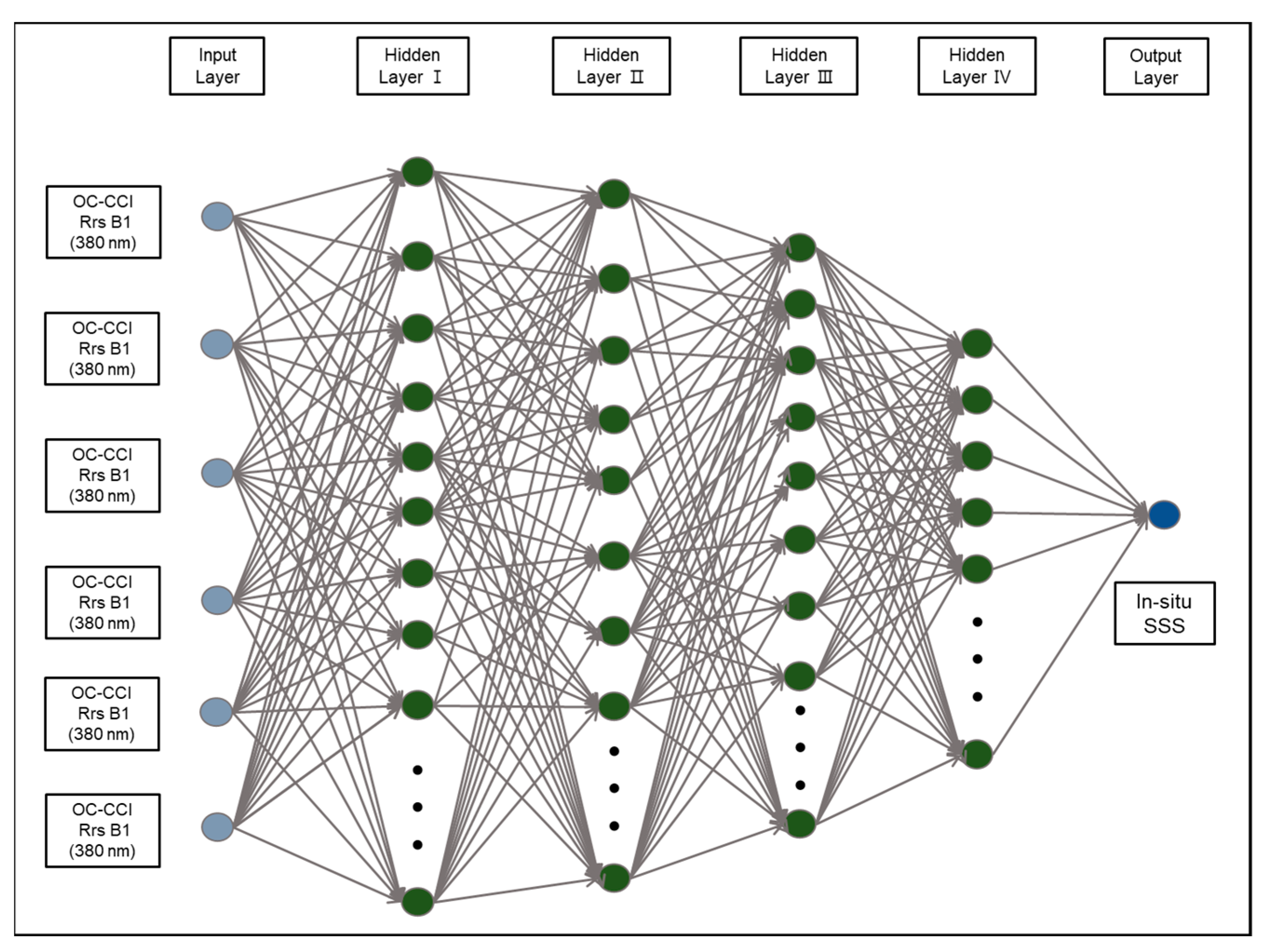
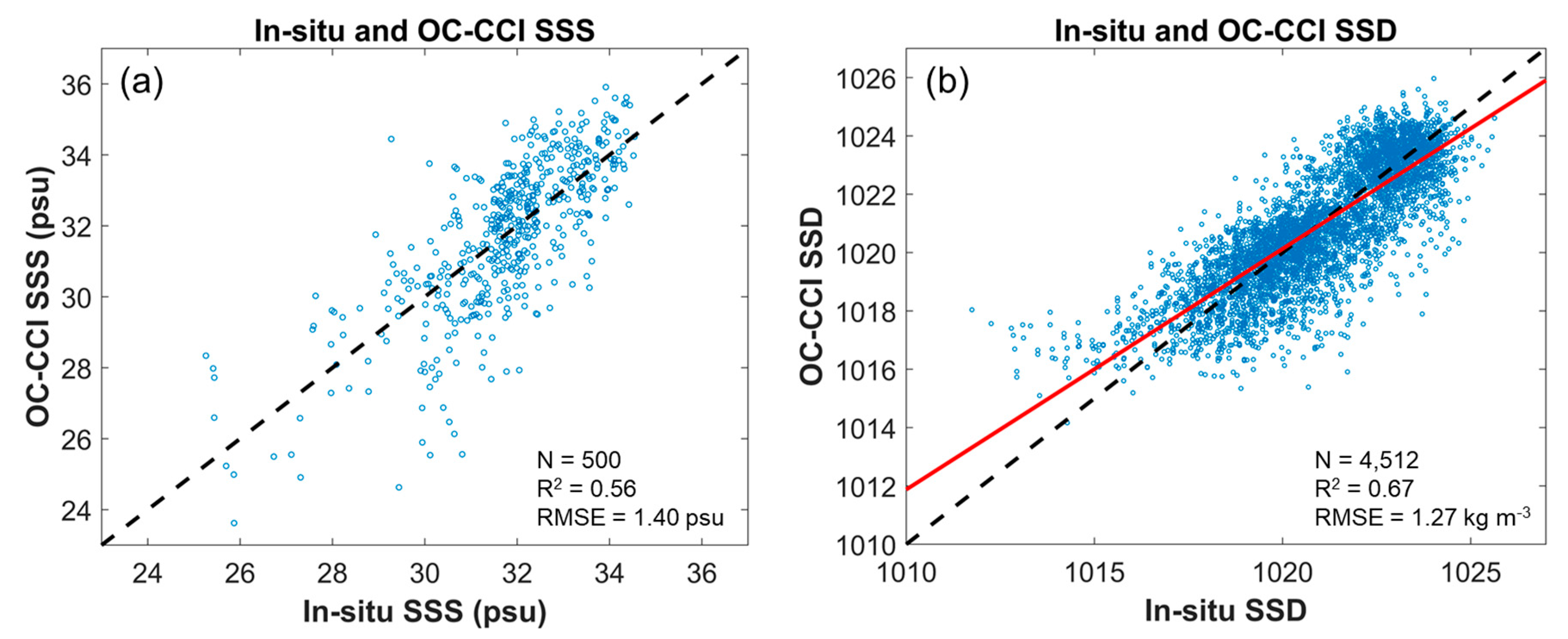
2.2. MPNN Model for SSS Estimation

Because the multi-layer perceptron neural network (MPNN) has been used to estimate SSS based on ocean color measurements in various regions [5,6,7,8], this method was adopted to develop an SSS estimation model for the OC-CCI. Because the shipboard survey stations are far from the Changjiang River mouth, the SSS range of in situ data lacking in the low-salinity conditions (under 25 psu). Thus, the model overestimates the Changjiang River mouth region, where the SSS is extremely low (<20 psu). Figure 2 shows an MPNN schematic diagram including six OC-CCI Rrs bands in the input layer and in situ SSS data in the output layer. To assemble two different datasets, the temporal resolution of in situ measurements was regarded as daily, and OC-CCI data were selected at the nearest location of the in situ survey stations. Thereafter, the datasets were randomly divided into training (80%) and validation (20%) datasets during the training period. The training was repeated 1000 times for each step while changing the number of hidden layers and neurons.
Figure 3a shows the performance of the MPNN model based on the validation dataset independent of the training dataset. The scatters were concentrated from 30 to 33 psu and R2 and root mean square error (RMSE) were 0.56 and 1.06 psu, respectively. Although the RMSE was acceptable, the SSS was corrected by the slope and bias owing to overestimation in the low SSS range (under 30 psu). After linear fitting, the overestimation and underestimation in the low and high SSS ranges were reduced despite the RMSE increasing to 0.34 psu. As the KNIFS serial shipboard survey stations are far from the Changjiang River mouth, an SSS under 25 psu was not obtained. Therefore, the accuracy decreased for low SSS values (under 30 psu). Given that the isohaline of the CDW in previous studies was 30 to 32 over the middle ECS [2,4,16,17], detection of the CDW fronts using our model near Jeju Island and the Korean Peninsula was possible. Moreover, the OC-CCI SSD was validated with KNIFS in situ measurements from 1997 to 2021 (Figure 3b). The R2 and RMSE between in situ and OC-CCI-based SSD were 0.67 and 1.27 kg m−3, respectively.

3. Results

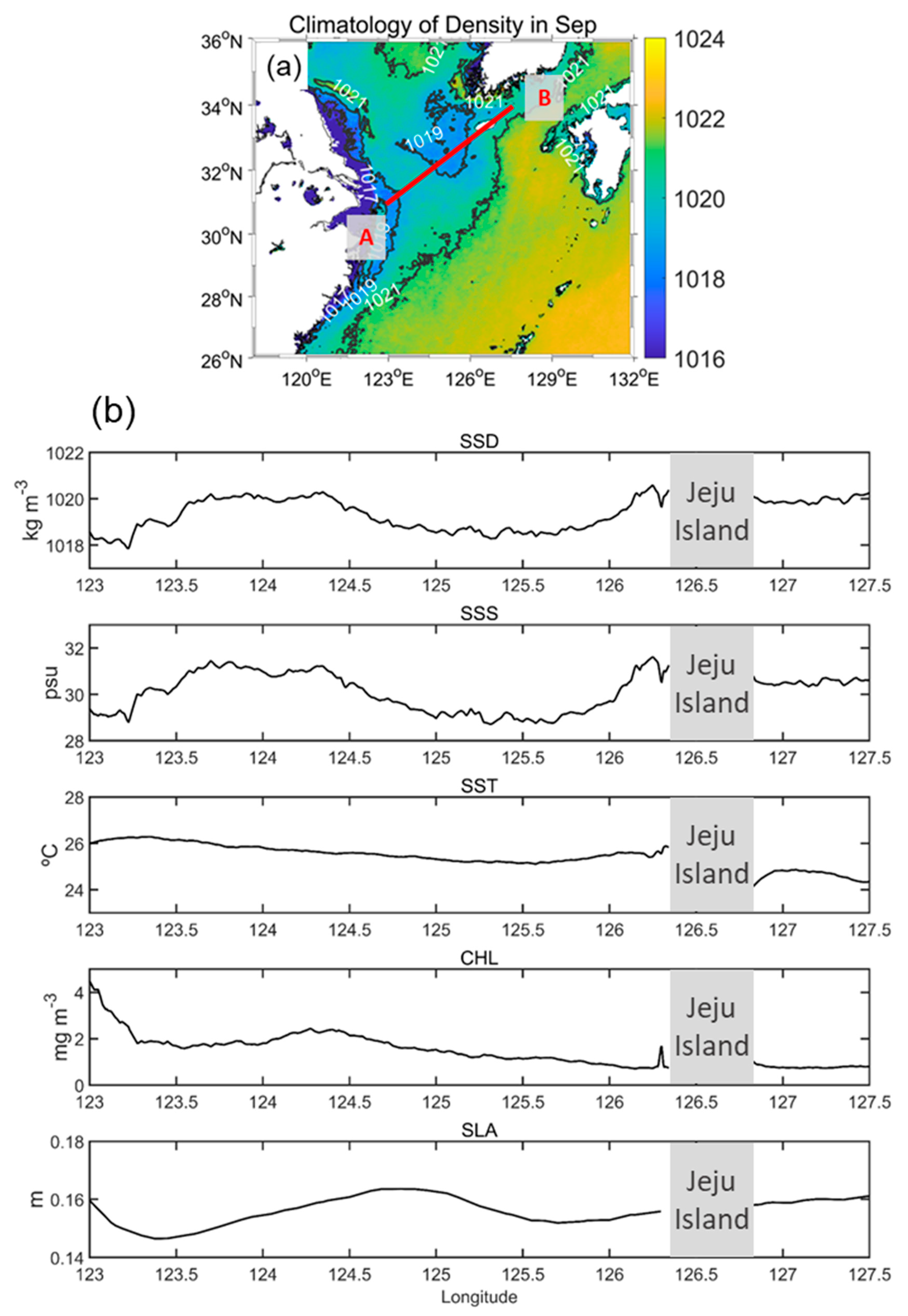
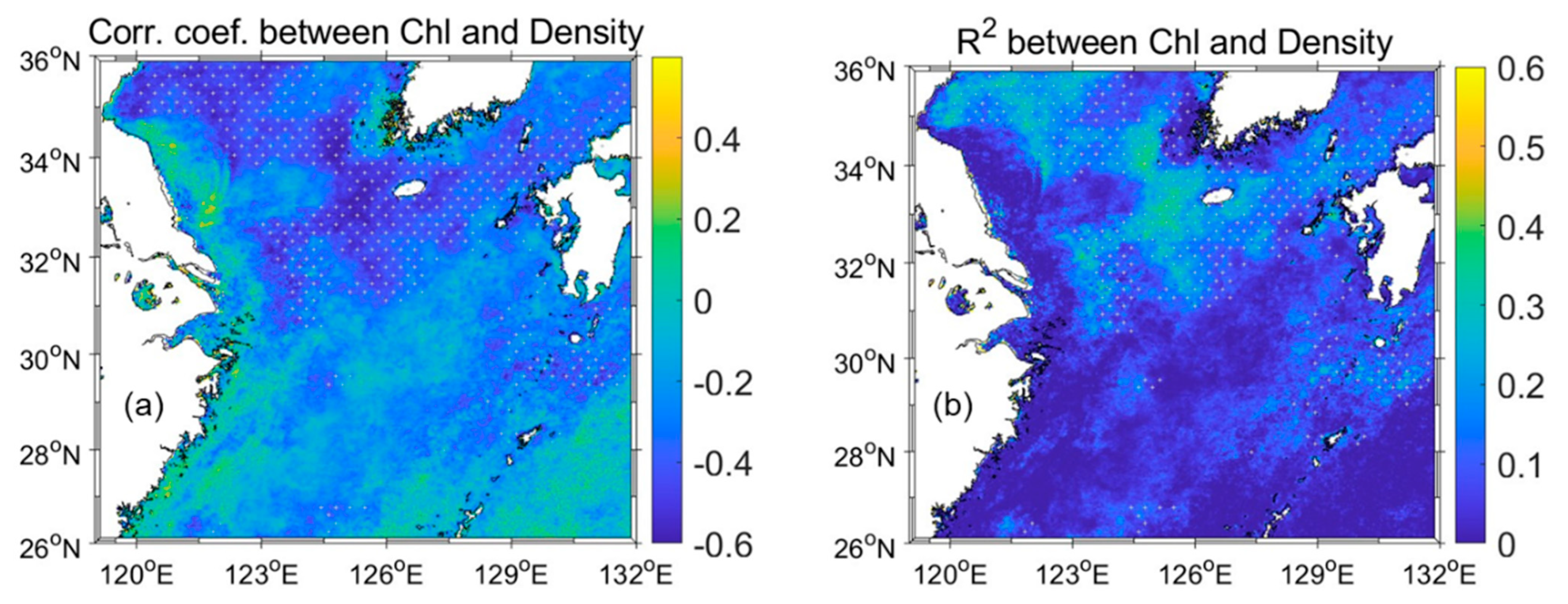
3.1. CDW Front Based on SSS, Chl, and SST

Because CDW rapidly evolves, factors such as gaps from frequent cloud cover, sun glint, and thick aerosols make it difficult to produce a monthly SSS distribution. However, it is possible to combine daily isohaline locations to produce cumulative isohaline footprints. Figure 4 shows the monthly cumulative isohaline footprints and monthly mean Chl concentrations from the June to September 2016 case as an example. The same figures from 1997 to 2021 are provided in the Supplementary Figures. The background color displays Chl; black dotted and solid lines and gray solid lines indicate 30, 31, and 32 isohaline footprints, respectively. The plume was generally directed northeastward, reaching Jeju Island, the Korean Peninsula, and sometimes the EJS through the Tsushima–Korea Strait. The isohalines are nearly parallel to the isobaths, especially the 50 m isobaths in June and the 100 m isobaths in the other three months (Figure 1). The plume shapes were in good agreement with the results of Bai et al. [2]. They presented the SSS distribution in July and August from 1998 to 2010 and identified three major types of extending shapes of the CDW based on the 31 isohalines. In August (Figure 4b and Supplementary Figures), the most apparent shape appeared as a type 2 plume in Bai et al. [2], which extends entirely northeastward, with the majority of the plume water traveling northward to the southern YS and then advected eastward through the Jeju Strait, with less low-salinity water remaining on the middle shelf of the southern ECS. However, the classification of the three types was not conducted owing to the ambiguous criteria. For example, mixed features appeared in August 2016 and the plume extended northeastward and southward.
The Chl distribution corresponded well with the isohaline footprints, despite not accumulating Chl. A probable reason for this is that the interaction between Chl and CDW had a time lag. Chl directly changes near the river mouth from the river origin Chl, but the rich nutrients in the CDW influence Chl within offshore regions [1,4,18]. This indicates that CDW could affect Chl for approximately one month. In addition, Chl rapidly decreased with increasing distance from the river mouth, unlike the isohalines pattern. This is because of complex situations, such as nutrient consumption, subsurface mixing, and the phytoplankton life cycle, which are difficult to demonstrate quantitatively in this study.
Figure 5 shows the climatology of SSS, Chl, and SST from June to September. The SSS and Chl were averaged from 1997 to 2021 (25 years), and SST was averaged from 2002 to 2021 (20 years) because the available data periods were different. Similar to CDW, the SSS and Chl fronts were distributed longitudinally. Chl and SSS showed river plume fronts, whereas SST did not. Near the Changjiang River mouth, SST formed ocean fronts longitudinally but was maintained up to 123°E. Except for this area, SST generated fronts latitudinally because of an insolation gradient. In addition, the CDW water mass, distinguished by 30 isohalines, was detached from the river mouth and transported to the Jeju Island. This detachment can be generated by the interaction between tide-induced vertical mixing and horizontal wind-driven movement of the CDW [19]. They determined the mechanism for the offshore detachment of the CDW using a three-dimensional numerical model. The detached patches in this study showed a pattern similar to the results of Moon et al. [19].

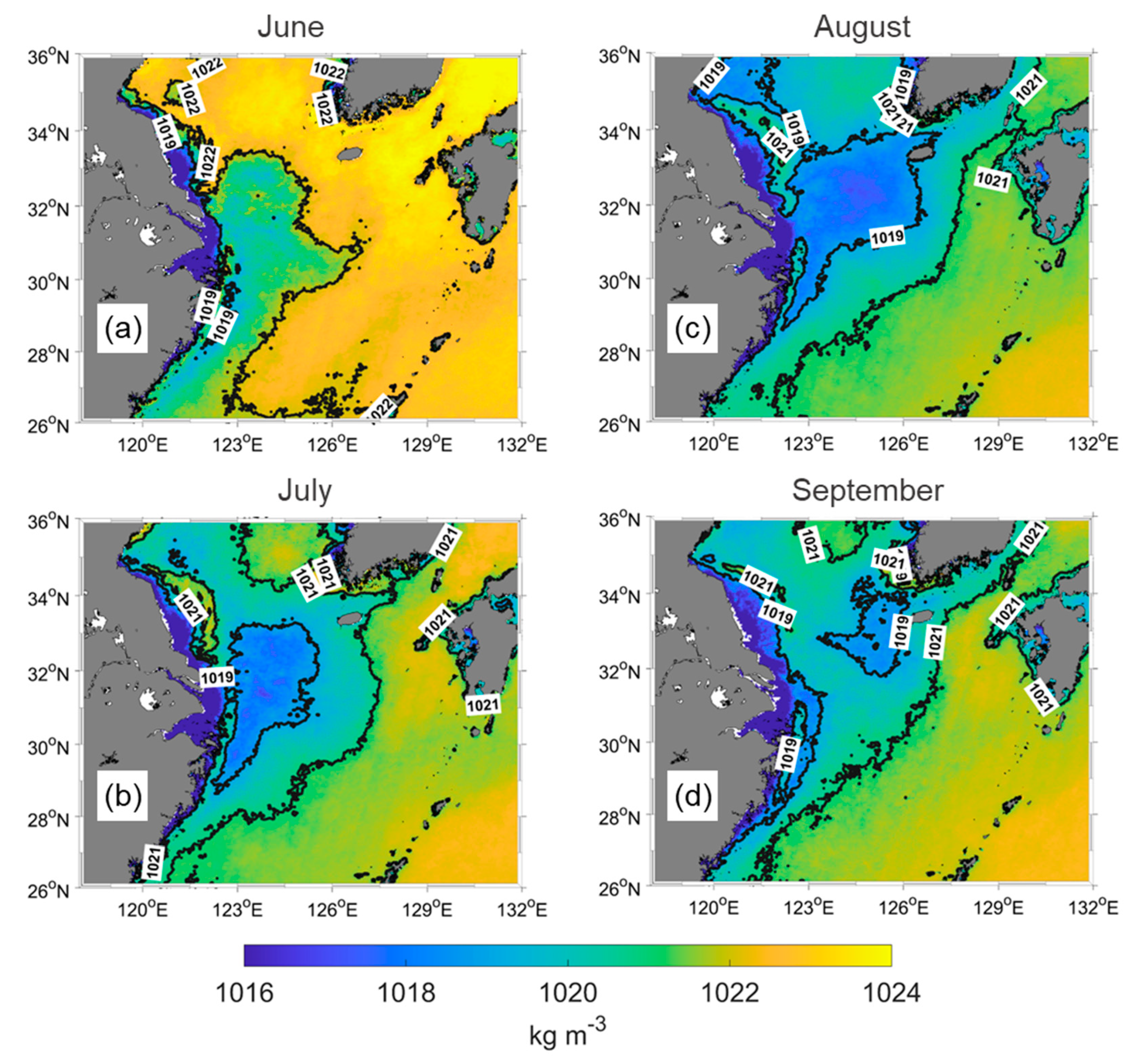
3.2. CDW Front Based on Surface Density

The different patterns of the various fronts suggest a complicated environment in the study area. Therefore, SSD was calculated using SST and SSS to distinguish CDW. Figure 6 shows the climatology of SSD from 2002 to 2021. The overall pattern seems similar to SSS (Figure 5a–d), but over the southeast of the CDW, it is different. This region is known as the high SST and SSS region because the Kuroshio Current is strong in summer. Because SSS is almost sustained in this area, SST increases from June to September, decreasing SSD by approximately 2 kg m−3. However, in the northern area, isopycnic lines follow isohalines, although the isothermal lines are obviously different. In September, the area of the 1019 isopycnic line (Figure 6a) was smaller than the area of 30 isohalines (Figure 5d) west of Jeju Island. However, detached patches were still clearly identified in the SSD distribution. During the summer, SSD decreased with increasing SST in the entire study region, but a noticeable reduction was observed in the CDW-dominated area.
Figure 7 shows the climatology of SSD in September for 20 years (2002 to 2021) and the SSD, SSS, SST, Chl, and SLA values along with a line originating from the Changjiang River mouth to the northeastern offshore region of the Jeju Island (AB line, presented in Figure 7a). The SSD shows a similar pattern to the SSS rather than the SST, indicating that SSS is a major factor driving SSD during September at this region. The detached SSD patch is also observed in Figure 7. The detached patch (high SSD and high SSS) was formed by tidal mixing with the subsurface, and ambient seawater covering due to the wind [19]. The Chl is at maximum at the river mouth and decreases toward B. However, the second peak of Chl appears around 124.3°E, where the SSD phase changes from high to low. This signifies that the Chl increased near the CDW front. Moreover, the SLA showed patterns similar to SSD. From the steric height variation perspective, the SLA evolved not only as water was added but also as SST or SSS evolved. In this case, the SSS variation could change the SLA since the SST is almost constant at 26 °C. When the SSD is high (low), SLA is low (high) because the water volume has a negative relationship with water density. However, the exact locations of the SSD and SLA peaks were slightly different. There are three possible causes: (1) the observed values were diminished by the 20-year averaging, (2) the spatial resolution of the SSD and SLA observations varied, and (3) the time lag between the SSD evolutions and the resulting SLA reaction. However, these assumptions are not clear. Consequently, additional studies are required to understand the relationship between SSD and SLA.
In addition, the correlation coefficient map and R2 map showed the regions where Chl was affected by SSD (Figure 8). A relatively high R2 (negative relationship) between Chl and SSD was observed near Jeju Island, the Yellow Sea, and the Tsushima–Korea Strait (p < 0.05). However, the other regions (particularly further south than 30°N) showed a low R2 at insignificant levels. Therefore, the SSD variation caused by SST changes did not influence Chl; however, the SSS changes contributed to regional Chl variation.

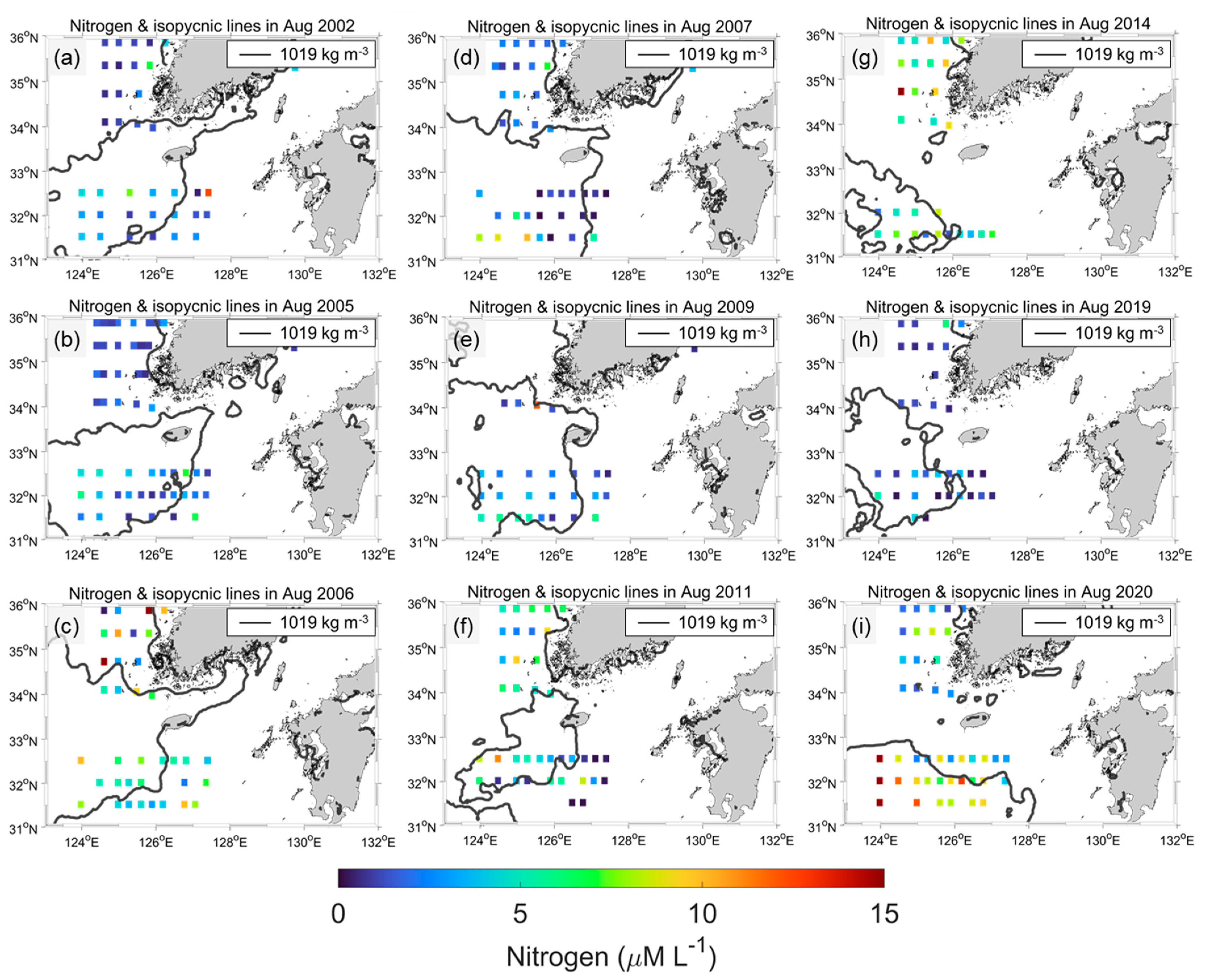
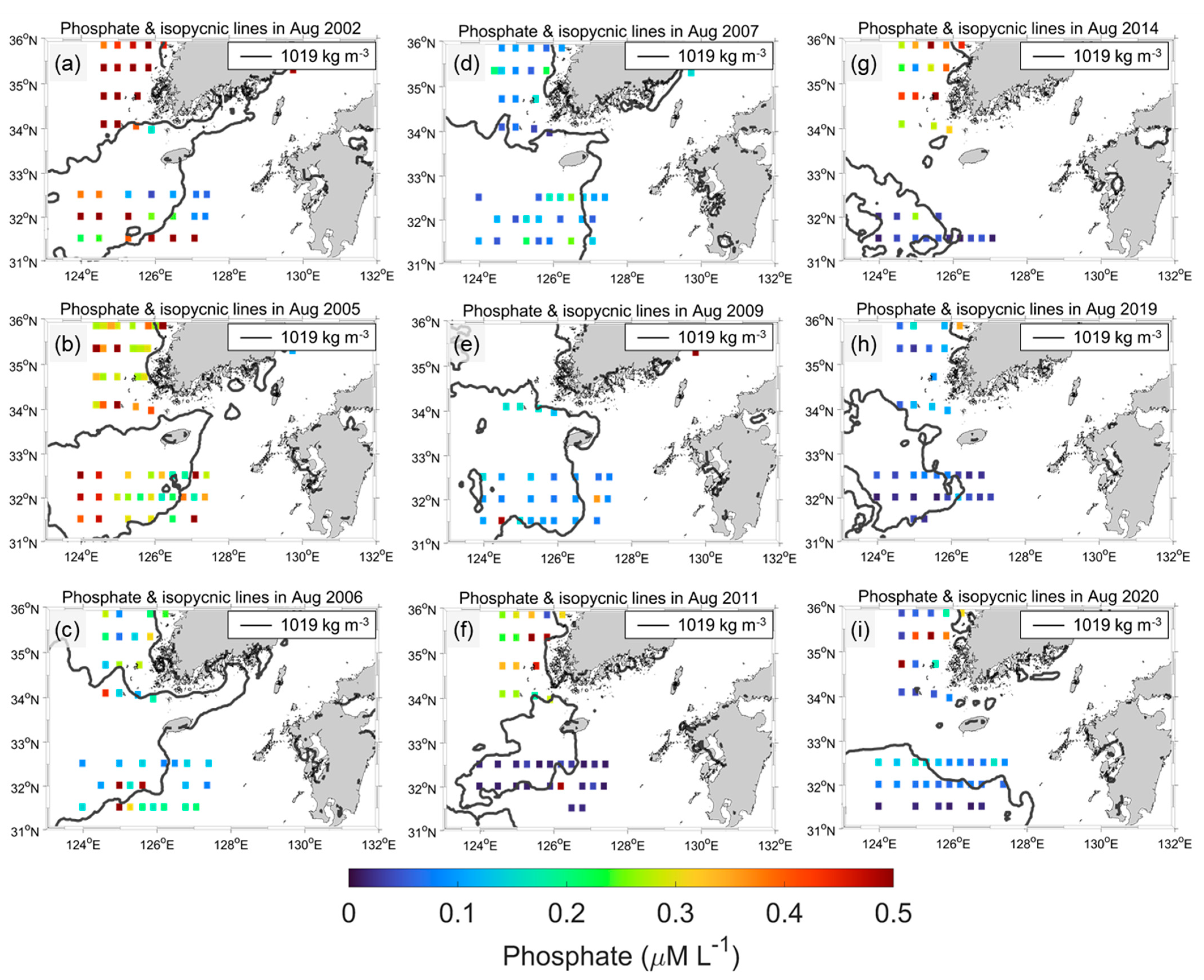
3.3. CDW Front for Nutrients’ Distribution

Because the CDW is rich in nutrients, the CDW extension transports nutrients over the ECS. Therefore, the nutrient conditions differed across the CDW front. In this study, the shipboard observed nitrogen (N) and phosphorus (P) concentrations, and the SSD fronts from satellite data were compared. Figure 9 and Figure 10 show the N and P levels with isopycnic lines in August for nine years (2002, 2005, 2006, 2007, 2009, 2011, 2014, 2019, and 2020) because the shipboard observations were conducted only in August at the ECS stations. In general, N was relatively high (4 to >10 μM L−1) at a low SSD, close to the Changjiang River mouth. N showed a different pattern across the 1019 isopycnic lines, indicating that the CDW had more N than ambient seawater. Because N was obtained only once at each station, in contrast with SSD, which was a monthly average, the comparison of the spatial distribution had some limitations. Nevertheless, clear differences were revealed in August 2005, 2007, 2011, 2014, and 2020, except for a few stations that showed relatively high (low) N inside (outside) of each 1019 isopycnic line. This indicates that the CDW is relatively rich in N from the river plume, and that the satellite-driven SSD can distinguish the front of N.
However, P did not follow the N and SSD spatial distributions over the nine year period. A high P inside the CDW cases was observed in 2002, 2006, and 2007 (Figure 10). In particular, P was relatively lower in the CDW interior than in the exterior during 2020, which was the opposite phenomenon in the case of N. Li et al. [20] determined the increasing N trend during the past 50 years in the ECS due to the Changjiang River plume; however, P has been nearly stable since 2000. Therefore, the N/P ratio increased, which contributed to changes in the phytoplankton community’s composition. Jiang et al. [21] obtained the same results in August 2009. They determined the factors that control the summer phytoplankton community in the ECS. This study examined phytoplankton blooms that caused enhanced eastward and southward CDW extension in August 2009. The diatoms and dinoflagellates bloomed under high N and low P conditions off the Changjiang Estuary. In addition, Zhou et al. [22] suggested that CDW plays an important role in diatom blooms by enhancing the pycnocline and P stress. Moreover, the coastal area adjacent to the Changjiang River Estuary is a high-risk region for harmful algal blooms [20,23,24]. Although the analysis of the phytoplankton community’s composition depending on the CDW front was not conducted in this study, satellite-driven SSD can be useful for the prediction of N and P distributions or major phytoplankton species before shipboard surveys.

4. Discussion

The SSS estimation model based on the OC-CCI ocean color measurements was developed using NIFS serial shipboard observation data. Although the in situ observation stations cover large regions, including the SSK and central ECS, the lowest SSS in these data was higher than 25 psu (see Figure 3a) because the stations were far from the Changjiang River mouth. Therefore, the model seldom estimated low SSS conditions (<20 psu) (Figure 5) despite being revealed near the Changjiang River mouth. Hence, the SSD in this area is underestimated. Bai et al. [2] also revealed this limitation. They used a simple analytical algorithm to estimate the SSS using the absorption of CDOM. The range of the in situ SSS was 26–36, and a low SSS (<28 psu) was not observed. However, such handling was not excessive owing to their interest in the variation in the CDW extension between 28, 29, 30, and 31 isohalines. Similarly, in this study, the middle range of SSS (29–32 psu) was used to analyze CDW identification and its impact; thus, the overestimation of low SSS was not significant. The training dataset contained abundant data in the middle SSS range, for which the model performance was relatively accurate (Figure 5). As shown in Figure 4, the monthly cumulative 31 isohalines were in good agreement with Chl fronts. As the cumulative SSS footprint was not influenced by low SSS (<20 psu), the results were reliable. However, the detached patches in July and August may have impacted the SSS (SSD) overestimation (underestimation) (Figure 5 and Figure 6). Thirty isohalines and 1019 isopycnic lines were separated from the Changjiang River mouth at 122.5°E, where the uncertainty was high. The overestimation (underestimation) of the SSS (SSD) produced a westward extension of the detached patches. Therefore, offshore CDW detachment occurred on the east side, and the area of the patch might have been much smaller than indicated.
To overcome these model limitations, more training datasets near the Changjiang River mouth region are required. Rarely obtained shipboard measurements are valuable for validating satellite-driven SSS products; however, they are insufficient for developing an SSS estimation model. Microwave satellite sensor-based SSS data can solve this problem. Kim et al. [5] and Kim et al. [6] avoided such limitations by using soil moisture active passive (SMAP) SSS data. Their model could estimate an extremely low SSS (<20 psu) near the Changjiang River mouth. However, it was difficult to develop the SSS estimation model for 25 years because SMAP data are available from 2015. Although the Soil Moisture and Ocean Salinity (SMOS) satellite has observed SSS since 2009, the low spatiotemporal resolutions and imprecision in coastal regions (a result of land interference) result in difficulties for its utilization in the ECS. Improving microwave SSS data quality in the ECS and assimilation with in situ measurements are recommended for further research.
In general, oceanic fronts are detected using specific algorithms, such as the histogram-based Cayula–Cornillon algorithm (CCA) and gradient-based Belkin–O’Reilly algorithm (BOA) [25]. However, these algorithms are unsuitable for investigating continuous front detection because they are highly sensitive to different parameter ranges. Therefore, the gradient-based fronts were inconsistent at different times. Therefore, the CDW fronts based on SSS and SSD were identified using thresholds (31 psu for SSS and 1019 kg m−1 for SSD). Although the thresholds were simply determined, previous research [2] supports the value of the threshold (31 psu), and effectively produced CDW fronts for 25 years.
This study was mainly conducted based on qualitative analysis because we focused on the spatial variation in marine environments caused by CDW. The spatial distribution of the CDW fronts explains the influence of CDW on Chl and DIN. However, to understand the mechanism and major factors of CDW behavior, more quantitative analyses are required in further studies. To conduct a quantitative analysis, more accurate SSS estimation and small-scale analyses are required. GOCI and GOCI-II measurements are valuable for small-scale analysis. Using high spatial (<500 m) and temporal (hourly) resolutions, more detailed analyses are possible, such as tides, small-scale eddies, wind, and typhoons.

5. Conclusions

In this study, an MPNN model for summertime SSS estimation in the ECS was developed based on satellite and in situ data from 1997 to 2021. Using time-series satellite-derived data, the monthly SSS, Chl, SST, and SSD fronts were presented and examined. The concurrence of SSS and Chl fronts indicated that CDW contributed significantly to Chl distribution in the ECS. In contrast, the SST fronts formed different patterns with Chl, indicating that the nutrients in the CDW were a major factor for Chl compared to the SST conditions during the summer months. CDW was identified in 31 isohaline and 1019 isopycnic lines. Detached patches were clearly revealed in the SSS and SSD distributions. In addition, N differences across the SSD fronts were observed. Although such an N distribution is possibly a consequence of CDW extension, more studies are required to explain the interaction between CDW extension and N.

Supplementary Materials

The following supporting information can be downloaded at: https://www.mdpi.com/article/10.3390/rs14153574/s1.

Author Contributions

Conceptualization, D.-W.K., S.-H.K. and Y.-H.J.; methodology, D.-W.K. and S.-H.K.; data curation, D.-W.K. and S.-H.K.; writing—original draft preparation, D.-W.K.; writing—review and editing, D.-W.K. and Y.-H.J.; visualization, D.-W.K.; supervision, Y.-H.J.; funding acquisition, Y.-H.J. All authors have read and agreed to the published version of the manuscript.

Funding

This research was supported by the Korea Institute of Marine Science & Technology Promotion (KIMST) funded by the Ministry of Oceans and Fisheries (20220546) and “Technology development for Practical Applications of Multi-Satellite data to maritime issues” funded by the Ministry of Ocean and Fisheries, Korea.

Data Availability Statement

Data sharing is not applicable to this article.

Acknowledgments

The authors acknowledge the Ocean Color Climate Change Initiative dataset, Version 5.0, European Space Agency, available online at http://www.esa-oceancolour-cci.org/ (accessed on 25 May 2022), for providing access to remote sensing reflectance products. We also thank the National Institute of Fisheries Science (NIFS) for providing in situ measurements, the Copernicus Marine Environment Monitoring Service for providing SLA data, and the Physical Oceanography Distributed Active Archive Center (PO.DAAC) of the National Aeronautics and Space Administration for providing SST data.

Conflicts of Interest

The authors declare no conflict of interest.

References

  1. He, X.; Bai, Y.; Pan, D.; Chen, C.T.; Cheng, Q.; Wang, D.; Gong, F. Satellite views of the seasonal and interannual variability of phytoplankton blooms in the eastern China seas over the past 14 yr (1998–2011). Biogeosciences 2013, 10, 4721–4739. [Google Scholar] [CrossRef] [Green Version]
  2. Bai, Y.; He, X.; Pan, D.; Chen, C.T.A.; Kang, Y.; Chen, X.; Cai, W.J. Summertime Changjiang River plume variation during 1998–2010. J. Geophys. Res. Ocean. 2014, 119, 6238–6257. [Google Scholar] [CrossRef]
  3. Chen, Y.; Hu, C.; Yang, G.P.; Gao, X.C.; Zhou, L.M. Variation and reactivity of organic matter in the surface sediments of the Changjiang Estuary and its adjacent East China Sea. J. Geophys. Res. Biogeosci. 2021, 126, e2020JG005765. [Google Scholar] [CrossRef]
  4. Kim, H.C.; Yamaguchi, H.; Yoo, S.; Zhu, J.; Okamura, K.; Kiyomoto, Y.; Tanaka, K.; Kim, S.W.; Park, T.; Ishizaka, J. Distribution of Changjiang diluted water detected by satellite chlorophyll-a and its interannual variation during 1998–2007. J. Oceanogr. 2009, 65, 129–135. [Google Scholar] [CrossRef]
  5. Kim, D.W.; Park, Y.J.; Jeong, J.Y.; Jo, Y.H. Estimation of Hourly Sea Surface Salinity in the East China Sea Using Geostationary Ocean Color Imager Measurements. Remote Sens. 2020, 12, 755. [Google Scholar] [CrossRef] [Green Version]
  6. Kim, D.W.; Kim, S.H.; Jo, Y.H. A Development for Sea Surface Salinity Algorithm Using GOCI in the East China Sea. Korean J. Remote Sens. 2021, 37, 1307–1315. (In Korean) [Google Scholar]
  7. Geiger, E.F.; Grossi, M.D.; Trembanis, A.C.; Kohut, J.T.; Oliver, M.J. Satellite-derived coastal ocean and estuarine salinity in the Mid-Atlantic. Cont. Shelf Res. 2013, 63, S235–S242. [Google Scholar] [CrossRef] [Green Version]
  8. Chen, S.; Hu, C. Estimating Sea surface salinity in the northern Gulf of Mexico from satellite ocean color measurements. Remote Sens. Environ. 2017, 201, 115–132. [Google Scholar] [CrossRef]
  9. Yan, W.; Zhang, S. The composition and bioavailability of phosphorus transport through the Changjiang (Yangtze) River during the 1998 food. Biogeochemistry 2003, 65, 179–194. [Google Scholar] [CrossRef]
  10. Zhang, J.; Liu, S.M.; Ren, J.L.; Wu, Y.; Zhang, G.L. Nutrient gradients from the eutrophic Changjiang (Yangtze River) Estuary to the oligotrophic Kuroshio waters and re-evaluation of budgets for the East China Sea Shelf. Prog. Oceanogr. 2007, 74, 449–478. [Google Scholar] [CrossRef]
  11. Gao, L.; Li, D.; Ishizaka, J.; Zhang, Y.; Zong, H.; Guo, L. Nutrient dynamics across the river-sea interface in the Changjiang (Yangtze River) estuary—East China Sea region. Limnol. Oceanogr. 2015, 60, 2207–2221. [Google Scholar] [CrossRef] [Green Version]
  12. Dai, Z.; Du, J.; Zhang, X.; Su, N.; Li, J. Variation of riverine material loads and environmental consequences on the Changjiang (Yangtze) Estuary in recent decades (1955−2008). Environ. Sci. Technol. 2011, 45, 223–227. [Google Scholar] [CrossRef] [PubMed]
  13. Kwon, H.K.; Kim, G.; Hwang, J.; Lim, W.; Park, J.W.; Kim, T.H. Significant and conservative long-range transport of dissolved organic nutrients in the Changjiang diluted water. Sci Rep 2018, 8, 12768. [Google Scholar] [CrossRef]
  14. Sathyendranath, S.; Grant, M.; Brewin, R.J.W.; Brockmann, C.; Brotas, V.; Chuprin, A. ESA Ocean Colour Climate Change Initiative (Ocean_Colour_cci): Version 3.1 Data; Centre for Environmental Data Analysis: Oxfordshire, UK, 2018. [Google Scholar]
  15. Mélin, F.; Sclep, G. Band shifting for ocean color multi-spectral reflectance data. Opt. Express 2015, 23, 2262–2279. [Google Scholar] [CrossRef]
  16. Su, Y.-s.; Weng, X.-c. Water masses in China seas. In Oceanology of China Seas; Springer: Dordrecht, The Netherlands, 1994; pp. 3–16. [Google Scholar]
  17. Chang, P.H.; Isobe, A. A numerical study on the Changjiang diluted water in the Yellow and East China Seas. J. Geophys. Res. Ocean. 2003, 108, 3299. [Google Scholar] [CrossRef]
  18. Chen, C.T.A.; Wang, S.L. Carbon, alkalinity, and nutrient budgets on the East China Sea. J. Geophys. Res. 1999, 104, 20675–20686. [Google Scholar] [CrossRef]
  19. Moon, J.H.; Hirose, N.; Yoon, J.H.; Pang, I.C. Offshore detachment process of the low-salinity water around Changjiang Bank in the East China Sea. J. Phys. Oceanogr. 2010, 40, 1035–1053. [Google Scholar] [CrossRef]
  20. Li, H.M.; Tang, H.J.; Shi, X.Y.; Zhang, C.S.; Wang, X.L. Increased nutrient loads from the Changjiang (Yangtze) River have led to increased harmful algal blooms. Harmful Algae 2014, 39, 92–101. [Google Scholar] [CrossRef]
  21. Jiang, Z.; Chen, J.; Zhou, F.; Shou, L.; Chen, Q.; Tao, B.; Wang, K. Controlling factors of summer phytoplankton community in the Changjiang (Yangtze River) Estuary and adjacent East China Sea shelf. Cont. Shelf Res. 2015, 101, 71–84. [Google Scholar] [CrossRef]
  22. Zhou, Z.X.; Yu, R.C.; Sun, C.; Feng, M.; Zhou, M.J. Impacts of Changjiang River discharge and Kuroshio intrusion on the diatom and dinoflagellate blooms in the East China Sea. J. Geophys. Res. Ocean. 2019, 124, 5244–5257. [Google Scholar] [CrossRef]
  23. Zhou, Z.X.; Yu, R.C.; Zhou, M.J. Resolving the complex relationship between harmful algal blooms and environmental factors in the coastal waters adjacent to the Changjiang River estuary. Harmful Algae 2017, 62, 60–72. [Google Scholar] [CrossRef] [PubMed]
  24. Qi, L.; Hu, C.; Liu, J.; Ma, R.; Zhang, Y.; Zhang, S. Noctiluca blooms in the East China Sea bounded by ocean fronts. Harmful Algae 2022, 112, 102172. [Google Scholar] [CrossRef] [PubMed]
  25. Belkin, I.M. Remote sensing of ocean fronts in marine ecology and fisheries. Remote Sens. 2021, 13, 883. [Google Scholar] [CrossRef]
Figure 1. Research region and matching stations for the in situ and OC-CCI data from 1997 to 2021. The serial shipboard observation stations were marked in green squares. The red, blue, and yellow arrows indicate warm, cold, and Changjiang outflow ocean currents, respectively, during summer season from 2002 to 2005 in this region (provided by Korea Hydrographic and Oceanographic Agency). Three bathymetric isobaths (50, 100, and 500 m) are also overlaid.
Remotesensing 14 03574 g001
Figure 2. The MPNN model architecture based on the OC-CCI Rrs six bands data and KNIFS serial shipboard measurements. Among the 2421 datasets, 80% were used to train, and 20% were used to validate model. The input datasets were fixed, and the number of hidden layers and neurons in hidden layers were varied to derive the best performance.
Remotesensing 14 03574 g002
Figure 3. (a) Linear fitting by slope and bias scatter diagrams between NIFS serial shipboard measurements and OC-CCI SSS. (b) Scatter plot between in situ and OC-CCI SSD. Red line indicates a linear regression line.
Remotesensing 14 03574 g003
Figure 4. Monthly Chl (shown with color map) and cumulative SSS footprint (shown with contours) from (ad) June to September 2016. The dotted and solid black and gray lines indicate 30, 31, and 32 isohalines, respectively.
Remotesensing 14 03574 g004
Figure 5. Climatology of OC-CCI (ad) SSS and (eh) Chl from June to September between 1997 and 2021. (il) Climatology of MODIS SST from June to September between 2002 and 2021.
Remotesensing 14 03574 g005
Figure 6. SSD climatology from June to September (ad) between 2002 and 2021. The CDW identified by 1019 isopycnic lines in the central ECS.
Remotesensing 14 03574 g006
Figure 7. (a) SSD climatology during September for 20 years (from 2002 to 2021). (b) Climatology for SSD, SSS, SST, Chl, and SLA along the A–B line (red line in (a)) during September.
Remotesensing 14 03574 g007
Figure 8. (a) Correlation coefficient and (b) R2 between Chl and SSD from 2002 to 2021. The gray cross symbols mark a p-value < 0.05.
Remotesensing 14 03574 g008
Figure 9. (ai) In situ nitrogen concentration (colored square) and 1019 isopycnic line during August 2002, 2005, 2006, 2007, 2009, 2011, 2014, 2019, and 2020. Nitrogen resulted from NIFS serial shipboard observations.
Remotesensing 14 03574 g009
Figure 10. (ai) Same as Figure 9 but phosphate during August 2002, 2005, 2006, 2007, 2009, 2011, 2014, 2019, and 2020.
Remotesensing 14 03574 g010
Table 1. The number of serial shipboard observations by Korean National Institute of Fisheries Science at the four regions from summertime (June to September) of 1998 to 2021. Among total 5488 data, about half (2421) data were matched with OC-CCI.
YearECS aSSK bYC cES d
1998261227734
1999221086819
2000321056820
2001331026820
200232986718
2003611086820
2004321086820
2005321086920
2006331086820
2007321106820
2008321106820
2009321086820
2010321084820
2011321086820
2012321086820
2013321086820
2014321086820
2015341086820
2016321086820
2017321086820
2018321086820
2019321086820
2020321086820
2021321086820
a East China Sea. b Southern Sea of Korea. c Yellow Sea. d East Sea.
Publisher’s Note: MDPI stays neutral with regard to jurisdictional claims in published maps and institutional affiliations.

