Article

Framework to Extract Extreme Phytoplankton Bloom Events with Remote Sensing Datasets: A Case Study

1
School of Marine Sciences, Sun Yat-sen University, Southern Marine Science and Engineering Guangdong Laboratory (Zhuhai), Zhuhai 519000, China
2
Key Laboratory of Spatial Data Mining and Information Sharing of Ministry of Education, National Engineering Research Centre of Geospatial Information Technology, Fuzhou University, Fuzhou 350108, China
3
Center for Remote Sensing, College of Earth, Ocean and Environment, University of Delaware, Newark, DE 19716, USA
4
State Key Laboratory of Marine Environmental Science, Xiamen University, Xiamen 361005, China
*
Author to whom correspondence should be addressed.
Remote Sens. 2022, 14(15), 3557; https://doi.org/10.3390/rs14153557
Submission received: 24 May 2022 / Revised: 10 July 2022 / Accepted: 21 July 2022 / Published: 25 July 2022

Abstract

:
The chlorophyll-a concentration (CHL) is an essential climate variable. Extremes of CHL events directly reflect the condition of marine ecosystems. Here, we applied the statistical framework for defining marine heatwaves to study the extremes of winter CHL blooms off the Luzon Strait (termed as LZB), northeastern South China Sea (SCS), from a set of remote sensing data. The application was enabled by a recent gap-free CHL dataset, the SCSDCT data. We present the basic properties and the long-term trends of these LZB events, which had become fewer but stronger in recent years. We further statistically analyze the LZB events’ controlling factors, including the submesoscale activity quantified by a heterogeneous index or surface temperature gradients. It was revealed that the submesoscale activity was also a vital modulating factor of the bloom events in addition to the well-understood wind and upwelling controls. This modulation can be explained by the stratification introduced by submesoscale mixed-layer instabilities. In the winter, the intensified winter monsoon provides a background front and well-mixed upper layer with replenished nutrients. During the wind relaxation, submesoscale baroclinic instabilities developed, leading to rapid stratification and scattered submesoscale fronts. Such a scenario is favorable for the winter blooms. For the first time, this study identifies the bloom events in a typical marginal sea and highlights the linkage between these events and submesoscale activity. Furthermore, the method used to identify extreme blooms opens up the possibility for understanding trends of multiple marine extreme events under climate change.

Graphical Abstract

1. Introduction

The South China Sea (SCS) is a subtropical large marginal sea with oligotrophic conditions. The ecosystem therein is characterized by nutrient limitations, strong seasonal variability, and complex physical and biological controls [1,2]. Off the northwestern Luzon Strait, winter blooms (hereafter, LZB) are a dominant feature of the ecosystem [3,4,5,6] and are featured with a high surface chlorophyll-a (CHL) concentration. The high winter CHL was contributed by both the photoacclimation process and the vertical mixing of subsurface CHL maxima [7]; nevertheless, the occurrence of LZB is a dominating ecosystem feature in the winter Luzon Strait. From the analysis of a large database of observed phytoplankton community structures, Liu, et al. [8] found a dominating role of nanoplankton for the LZB, accounting for >40% of the total CHL. For the more oligotrophic condition in the summer, picoplankton became dominant. In recent years, growing interest has been devoted to the LZB, mostly because of its complex controls and modulations by various dynamic factors such as the Kuroshio [9] and nonlinear subsurface upwelling [10]. These studies have reached a consensus that the primary driving force of LZB is the (seasonal) monsoon-induced winter mixed-layer deepening [5,6], while local circulations (including rotational mesoscale circulations, i.e., eddies) or the Ekman dynamics [11] provide the additional vertical nutrient inputs from the subsurface layers below the nutricline [12]. To summarize, previous studies have extensively investigated the link between LZB and multiple controlling factors, such as the wind, SST, mixed-layer entrainment, and Ekman dynamics, at the seasonal [6] or interannual [11] scales. Most of the existing studies focus on some particular events of LZB, explaining their controlling dynamics with process-oriented approaches [3]. There are, however, very limited studies that analyzed the LZB from the perspective of averaged properties across multiple bloom events. Little attention has been devoted to systematically investigating the generalized properties and controlling factors of multiple LZB events.
Submesoscale processes are a wide category of processes [13,14] at the scale of 0.1–10 km [15,16], which are often associated with the intense vertical movement or mixing of water. In many other oceans, submesoscale processes have been shown to intensively perturb the ocean ecosystem, leading to extraordinary phytoplankton blooms [17] or the export of organic carbon [14]. In the SCS, the physical aspects of submesoscales have been increasingly investigated [18,19,20,21], but their role in the ecosystem has seldom been investigated. Due to the limitation of the resolution of remote sensing and the difficulty of in situ sampling, numerical models are primary tools for studying the ecosystem response to submesoscale activity [22,23,24,25,26,27]. Nevertheless, a variety of studies utilized remote sensing data to study submesoscale activity, mostly with the temperature or CHL product that has sufficient resolutions [28,29,30,31,32,33]. Liu and Levine [31] developed a statistic tool, the heterogeneity index (HI), to quantify the intensity of submesoscale activity from high-resolution remote sensing and found that submesoscale frontal dynamics can enhance CHL as compensation for surface temperature warming. Ni, et al. [32] extracted “cat’s eye” shaped submesoscale eddies in the SCS with ocean color images and found a wide distribution of such structures in the marginal SCS. Guo et al. [9] have statistically linked LZB to submesoscale fronts, especially at the interannual scales. However, how the submesoscale activity contributes to CHL blooms in the SCS remains unclear.
Recently, a statistic framework has been proposed by Hobday, et al. [34] to study marine heatwaves (MHWs) from long-term daily products (hereafter, the H16 framework). As an emerging research area, this framework has been increasingly applied to understand the spatio-temporal distribution, long-term trends, and climatic links of MHWs [35,36]. Despite its extensive applications [37], this framework has rarely been applied to understand the extremes of biogeochemical essential climate variables [38] such as chlorophyll-a concentration (CHL). The understanding of ocean extreme events and associated impacts on the ecosystem remains limited [39]. The extremes of CHL directly reflect the health of marine ecosystems and their capability to provide goods and services. This is particularly important given the background of climate change impacting marine ecosystems [40].
One essential factor hindering such studies is the fact that only ocean color remote sensing data could provide the required daily resolution long-term dataset for the H16 framework, but these data are susceptible to cloud contaminations and often have a high missing rate. This is particularly true for marginal seas such as the SCS, which is masked by clouds all year round [41]. To overcome this issue, our previous study proposed a Discrete Cosine Transform (DCT) reconstruction method, yielding a full daily 4 km CHL product named SCSDCT [42]. The details of SCSDCT will be presented in Section 2.1.
To summarize, in order to bridge these knowledge gaps, we ought to apply the H16 framework with the SCSDCT dataset to extract and understand the interannual variabilities and long-term trends of the LZB events. This paper is organized as follows. In Section 2, we present the datasets applied in this study, as well as the details of the H16 framework. In Section 3, descriptions of these bloom events are presented, particularly focusing on the strongest 2014 event. In Section 4, we discuss the long-term trends and controlling factors of the bloom events. In Section 5, the main findings of this study will be summarized, with a discussion on the future direction of related studies.

2. Data and Methods

2.1. Datasets

2.1.1. Remote Sensing Reconstruction: SCSDCT

The core dataset utilized in this study is the SCSDCT CHL product detailed in Wang et al. [42], which will be briefly introduced here. It was originally developed for the adjacent Luzon Strait. We validated SCSDCT particularly for the northern SCS region; we will focus on the adjacent LZB region. The SCSDCT applied the gap-filling method DCT to reconstruct the Ocean Color Climate Change Initiative version 4.2 daily 4 km surface CHL concentrations product (OCCCI, http://www.esa-oceancolour-cci.org, accessed on 1 May 2022), which is a merge of multiple optic sensors. For the northern SCS, the OCCCI data have an overall missing rate of 81.5%. In our previous study, the reconstructed SCSDCT was especially validated with in situ CHL data from northern SCS and was shown to perform better than other reconstruction methods in representing the intraseasonal (30- to 60-day) variabilities of winter CHL in the adjacent LZB regions. The reconstruction has shown its capability to more robustly reflect the intraseasonal variabilities of CHL from intraseasonal Madden-Julian Oscillation by avoiding biased sampling in the original gapped data [42]. Compared with the observation from [43], SCSDCT has a root-mean-squared error of 0.148 mg m−3 and an R2 of 0.60. By comparing the in situ data with the original OCCCI (i.e., those not masked by clouds), the root-mean-squared error is 0.104 mg m−3 and the R2 is 0.76, which is the upper limit of the reconstruction. The dataset is publicly distributed on the Science Data Bank (https://doi.org/10.11922/sciencedb.01066, accessed on 1 May 2022). The original OCCCI data are also applied to assist in the analysis. The CHL averaged over the offshore box (the small box in Figure 1a) is used to quantify LZB, which was considered representative of previous studies [3,4]. Unless otherwise indicated, the bloom event in the text refers to the area-averaged LZB event, and winter means the months of November through February, while the time span for the climatology is 2005–2019.

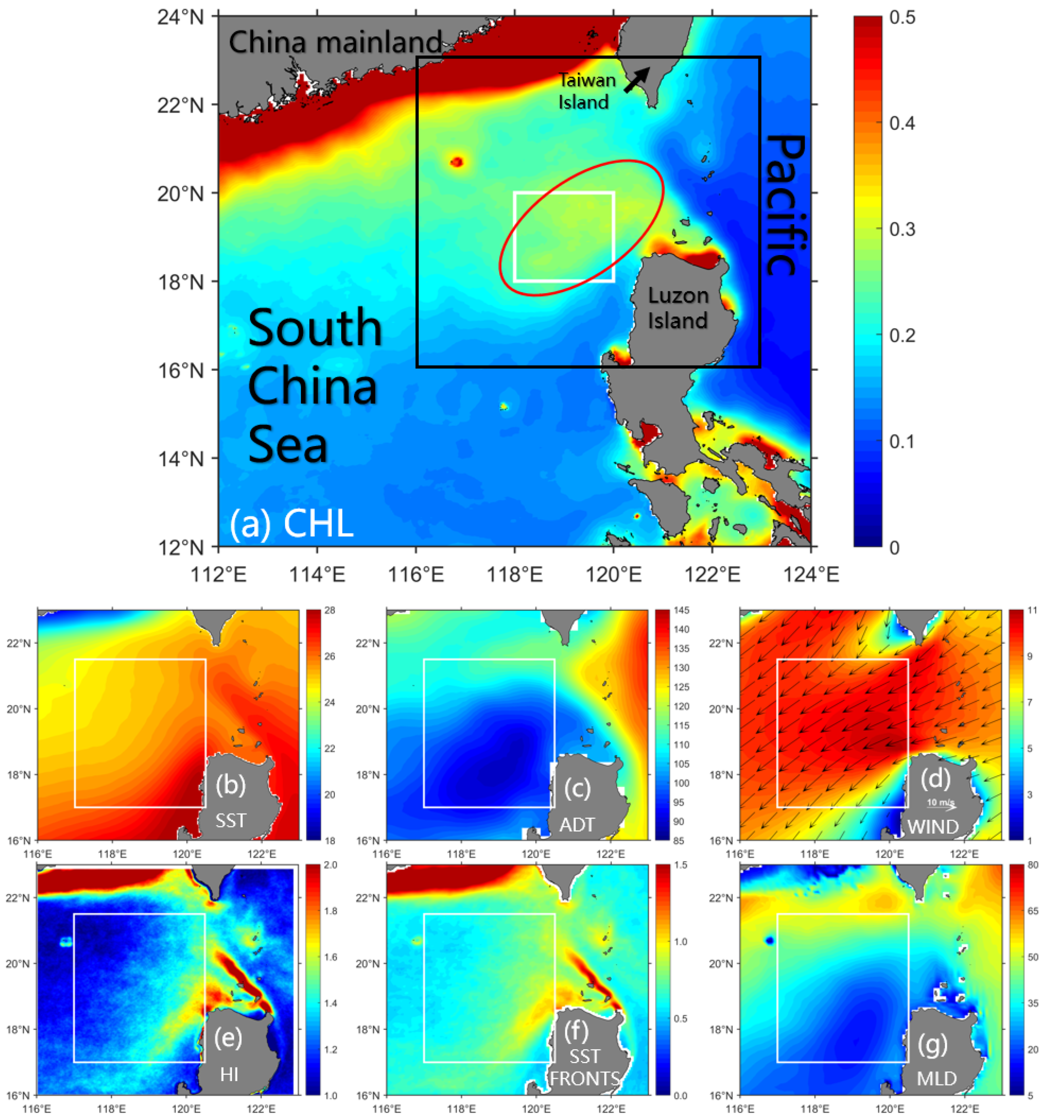
2.1.2. Other Products: Controlling Factors

To facilitate the discussion of controlling factors of bloom events, we use datasets including remote sensing sea-surface temperature (SST), sea surface height (SSH), 10 m winds from atmospheric reanalysis, and mixed-layer depth (MLD) from ocean reanalysis. These data sets are summarized in Table 1. SST is from the Multi-scale Ultra-high Resolution (MUR) Sea Surface Temperature dataset derived by JPL at https://podaac.jpl.nasa.gov/MEaSUREs-MUR?sections=data (accessed on 1 May 2022). The SSH is derived from satellite altimeters from the Absolute Dynamic Topography products of the Archiving, Validation, and Interpretation of Satellite Oceanographic (AVISO) data project (https://resources.marine.copernicus.eu, with a data label of SEALEVEL_GLO_PHY_L4_REP_OBSERVATIONS_008_047, accessed on 1 May 2022). The 10 m winds, including the meridional and zonal components, are from the state-of-the-art ERA5 (fifth generation of the European Center for Medium-Range Weather Forecasts atmospheric reanalyses of the global climate) reanalysis from Copernicus Climate Change Service (https://cds.climate.copernicus.eu/, accessed on 1 May 2022). The MLD is from the 1/12-degree global reanalysis product from the Copernicus Marine Service.
Using the method proposed by Liu and Levine [31], we derive the HI (Heterogeneity Index) from MURSST to reflect the contribution from submesoscale processes, which were shown to modulate the LZB by previous modeling work [9]. The HI can be expressed as:
H I = a ( b | γ | + c σ n + d P )
P = m i n ( x ) m a x ( x ) | p ( x ) g ( μ , σ ) | g ( μ , σ ) d x
In the equations, γ is the skewness of the SST distribution and σ is the standard deviation, both representing that of SST in a 10 by 10 spatial box with n = 100. p(x) is a five-order polynomial function fitted from SST, while g(μ, σ) is the best-fit Gaussian function with the sample mean of μ and the standard deviation of σ. The difference between the two fitting functions represents the deviation of SST distribution from the normal distribution, which is considered to be perturbated by small-scale processes such as submesoscale activity. The factors b, c, and d adjust the relative contribution of each term so that they contribute approximately equally over the whole domain, while the factor a normalizes HI to [0, 1] so that HI = 0 represents the homogeneous regime and HI = 1 for the greatest heterogeneity.
The SST frontal intensity was also calculated from MUR SST, with a gradient detection method developed by Belkin and O’Reilly [44]. Specifically, a median filter was applied first, which is to smooth the edges and leave the sharp extrema at the same time. The Sobel operator, which consists of two 3 × 3 convolution windows, WX and WY (Equation (3)), was used to detect the gradient vector. The result of the convolution operation in the x and y axes was represented by G x and G y , respectively. The frontal intensity equals: (Equation (4)).
W X = [ 1 0 1 2 0 2 1 0 1 ] ,   W Y = [ 1 2 1 0 0 0 1 2 1 ]
F r o n t a l   I n t e n s i t y = ( G x 2 + G y 2 )
To analyze the bloom events, all these datasets in Table 1 had a daily resolution from 2005 to 2019. A spatial average of CHL was used to characterize the LZB (Figure 1a), while those controlling factors are averaged in a larger box (Figure 1b–f). Since spatial average or composite maps will be applied, the difference in spatial resolution is not a concern.

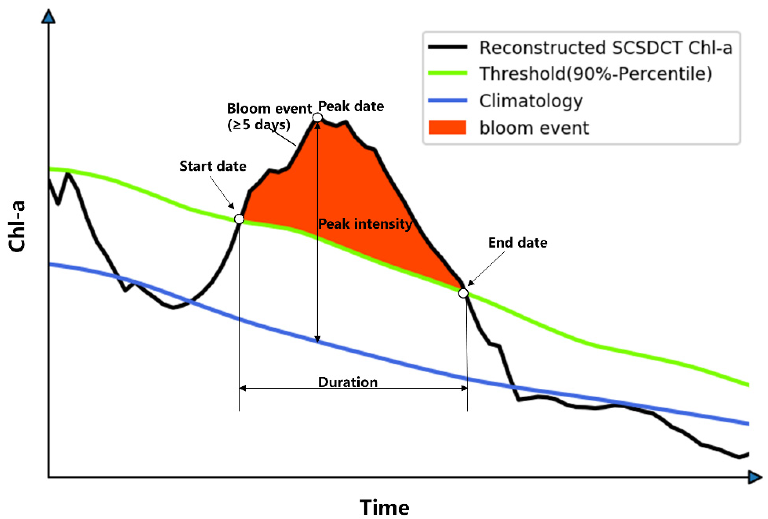
2.2. Method: H16 Framework for Marine Heat Waves

We adopted the framework of analyzing MHWs by Hobday, et al. [34] (hereafter, H16). The H16 framework defines MHWs as a discrete period of prolonged, anomalously warm water at a particular location [37]. Statistically, an MHW event is defined if the temperature is higher than a seasonal-varying daily threshold at a particular location [34]. Similarly, bloom events can also be defined. In this study, we identified LZB events from the 15-year records of DCT-SCS reconstruction. For each day of the year, CHL data from the adjacent 11-day window for all 15 years were accumulated to a probability distribution, from which a threshold value was defined as the 90th percentile. This annual cycle of thresholds was further smoothed with a 31-day moving window. If the CHL was higher than the threshold for more than 5 days, a bloom event is identified as occurring. Figure 2 illustrates one example of a bloom event. In this study, we adopted the H16 codes from GitHub at https://github.com/ecjoliver/marineHeatWaves (accessed on 1 May 2022). The statistical matrix of the events includes the duration (in days), maximum intensity (in mg m−3), mean intensity (in mg m−3), and accumulated intensity (in mg m−3 days). As a first step, the analysis will focus on the spatial averaged LZB events and corresponding composite, except for the pixelwise trends in Section 3.3 (see below).

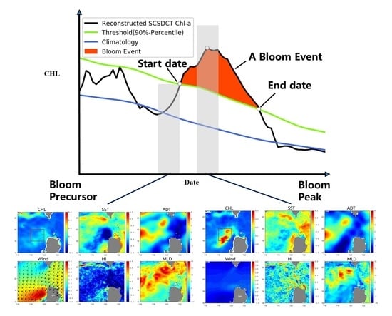
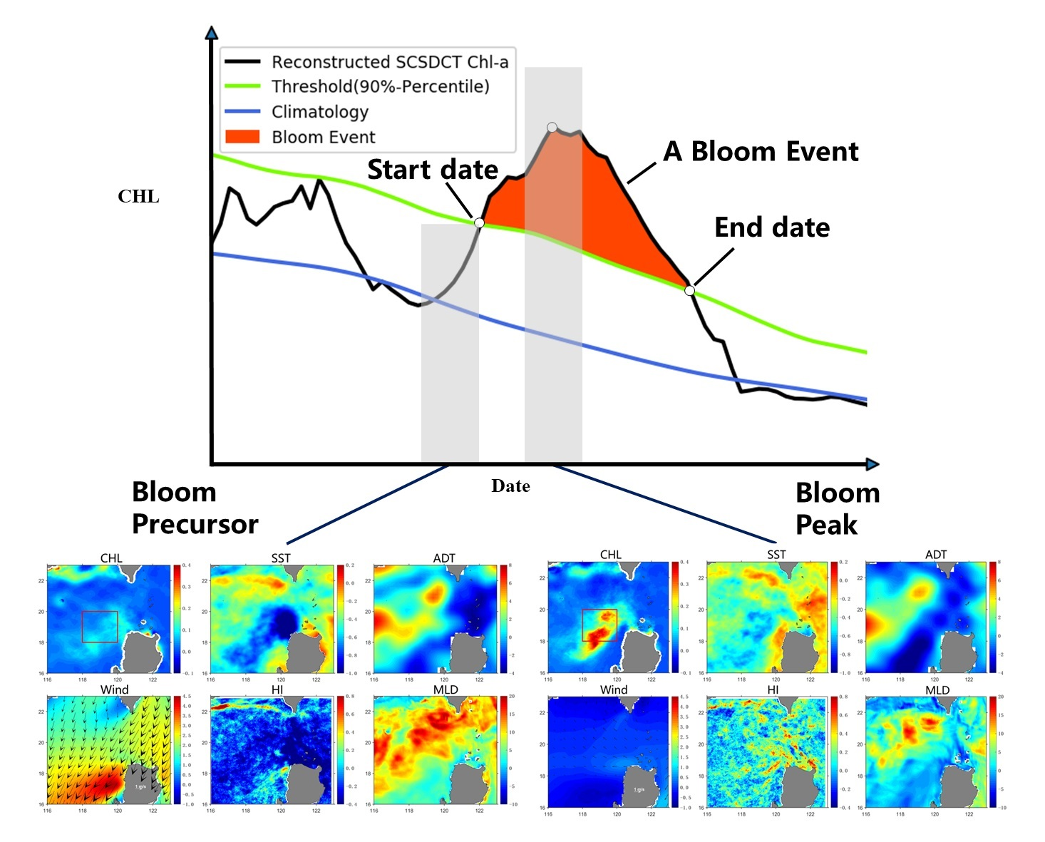
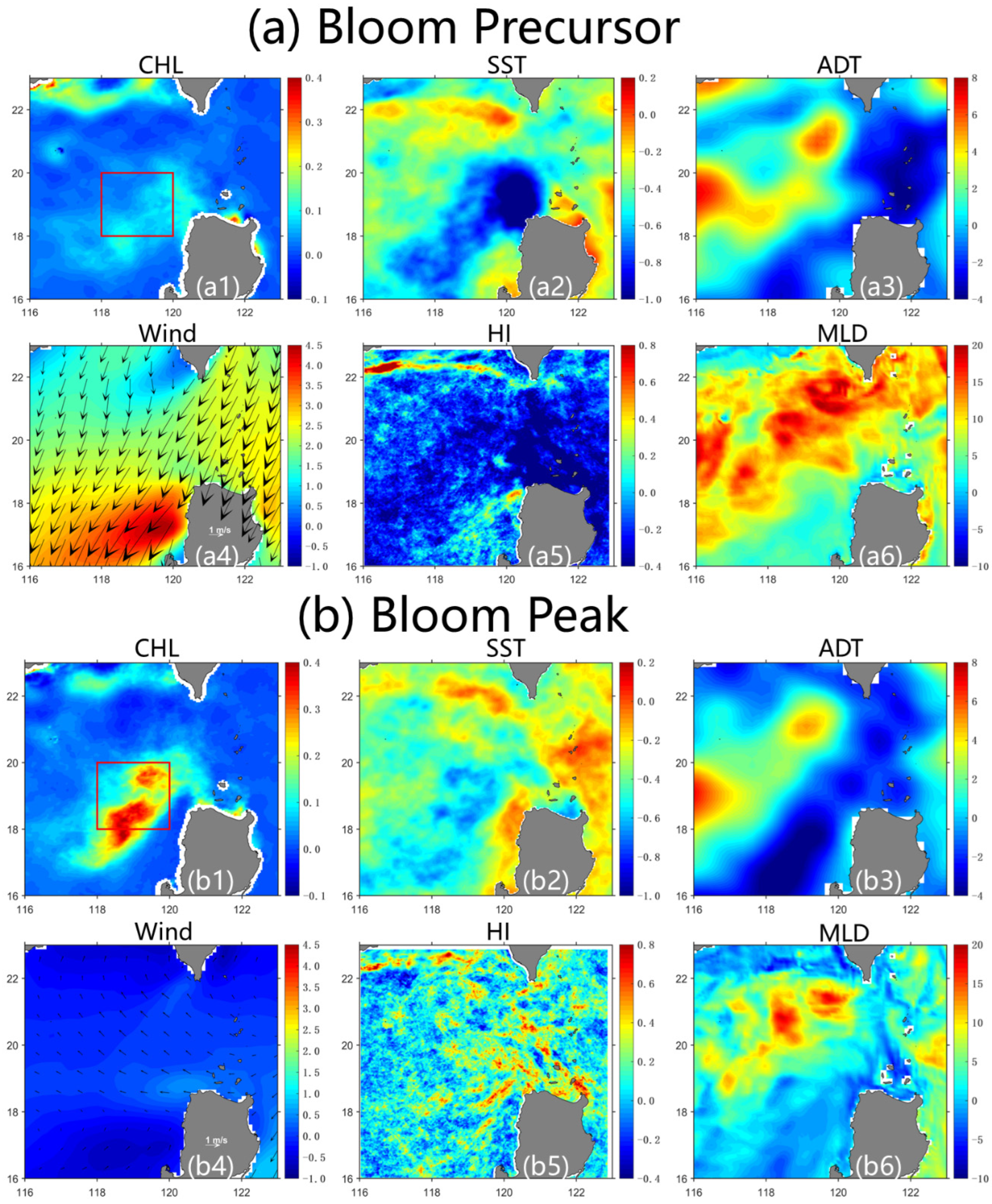
2.3. Method: Bloom Composite

To summarize many LZB events in a clear way, and to link the occurrence of events to the environmental factors, we use a composite method. After extracting LZB events (especially the day of occurrence) with the H16 framework, a normalized event could be derived by matching all events according to their starting, peaking, or ending days. Then, the average can be taken across all events to yield a normalized event. Since general interests are in the genesis of blooms, we choose the initial days to match all bloom events. In other words, we temporally matched all blooms according to the onset (initial) day so that day 1 refers to the first day of each bloom. The CHL and corresponding controlling factors were then averaged to derive a normalized bloom event (one single CHL anomaly time series with corresponding controlling factors’ time series). For this normalized event, a lag correlation can be then applied to understand the controlling effects, with a maximum lag of 7 days (controlling factors lead the CHL). An optimal lag of maximum correlation can be identified for each factor.

3. Results

3.1. Bloom Events Defined via H16

We first present the LZB events extracted via the H16 framework. Noting that these events are from the area average of the small box in Figure 1a. From Figure 3, a general seasonal cycle is lower in the summer and higher in the winter (as high as 0.5 mg m−3). As a result, the threshold for LZB is also much larger (~0.1 mg m−3 CHL anomaly) than that in the summer. From 2005 to 2019, a total of 12 LZB events were identified. Among the 12 events, most (9 events) occurred in December, one occurred in November, and two occurred in January. Except for 2007, 2011, and 2014, only one or zero LZB events took place each winter. Some of these events were previously reported, such as the December 2007 or January 2010 events [5,9], but some have seldom been investigated.
Figure 4 summarizes all the LZB events in the period of 2005–2019, including the duration (Figure 4a), maximum intensity (Figure 4b), cumulative intensity (Figure 4c), and mean intensity (Figure 4d). The maximum bloom intensity (mean bloom intensity) for these 12 bloom events has a mean value of 0.27 (0.16) mg m−3. The duration days of all bloom events range from 5 to 14 days, with an average duration of 9.8 days. The long LZB events occurred in the years 2008, 2010, 2012, and 2014. Among these years, 2008 and 2010 are both La Niña years. During the La Niña years, the winter-averaged CHL concentration off the Luzon Strait was higher [9], but the La Niña year is not a sufficient condition for the occurrence of extreme LZB events. In fact, a correlation analysis of all four LZB matrices (those in Figure 4, N = 12) versus the monthly Multivariate El Niño-Southern Oscillation Index (MEI) did not find any significant correlation, regardless of there being a lag (from 0–12 months) or not. This implies the complexity of marine blooms, which are driven by multiple factors.
Moreover, this duration implies that the practical sampling interval for LZB events, on average, is 2.45 days (twice the Nyquist’s Theorem of the sampling requirement, [47]), which is shorter than the available Level-3 optic datasets such as the original OCCCI product (considering the data missing due to cloud masking). Therefore, using reconstructed data is the only feasible way to monitor marine bloom events for marginal seas such as the SCS. In 2014, all indexes suggested that the event is the strongest in 15 years, with a maximum bloom intensity of 0.84 mg m−3.

3.2. Event of 2014 Winter
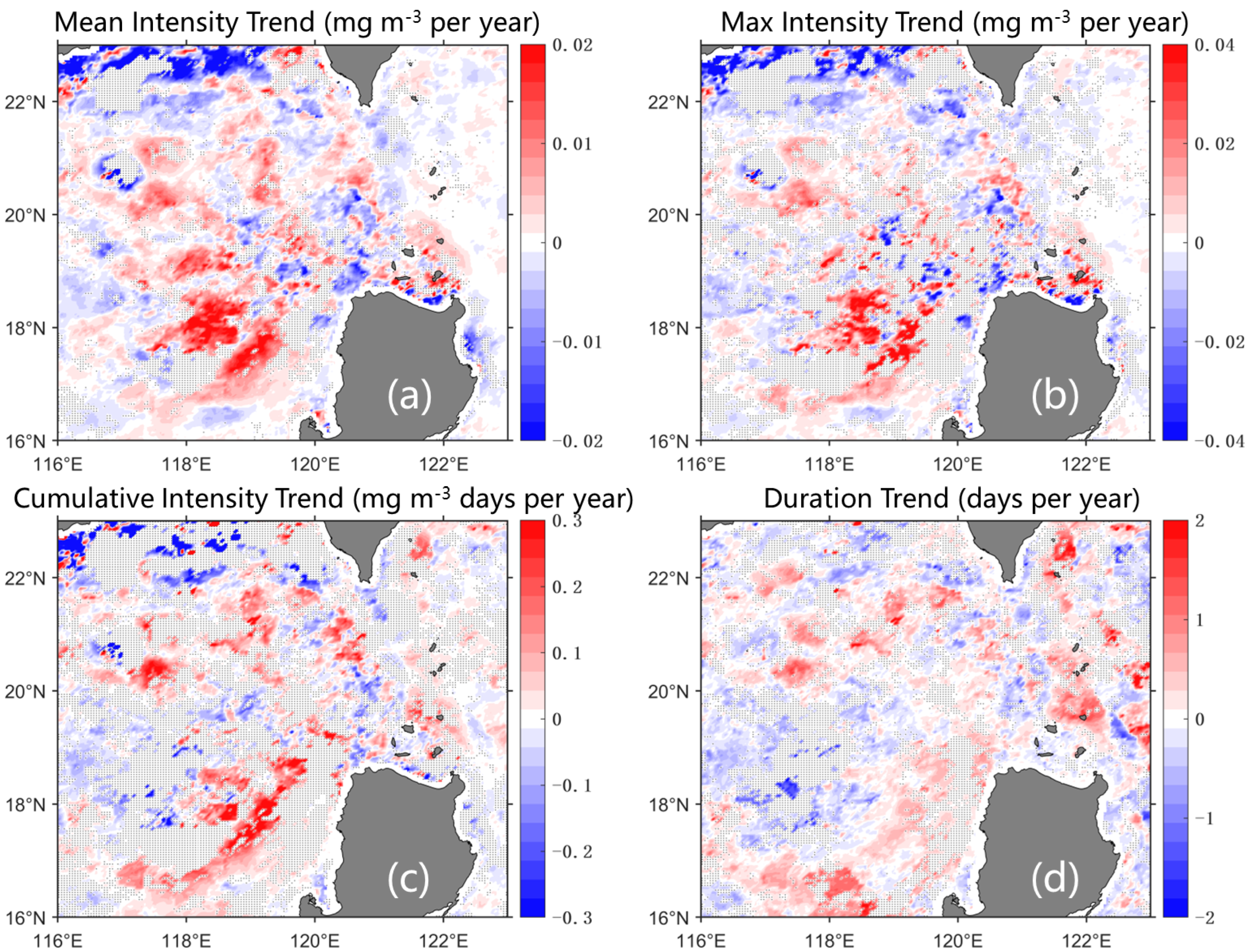
From the 20th of January to the 2nd of February, 2014, an extremely strong LZB event occurred, as defined by the area-averaged time series of CHL. From corresponding spatial maps (Figure 5), it was clear that the bloom initiated from a small offshore bump clinging to the northwestern tip of Luzon Island. Later, the bloom evolved and started to flourish in the shape of an inversed-V structure [4]. During these phases, the SST and SSH generally showed cold and upwelled water, but the cooling center mismatched the bloom center (Figure 6). This was also the case for, for example, the Jan 2010 case we previously investigated [5]. We proposed the occurrence of subsurface upwelling, which could not be directly detected from surface signals. For the 2014 case here, the pixelwise CHL concentration peaked at a maximum concentration > 6 mg m−3 (for original OCCCI data that are not shown in figures but can be easily accessed from https://www.oceancolour.org/portal/, accessed on 1 May 2022). For the SCSDCT, the CHL was weaker, but there was a CHL anomaly above the 90th threshold for >0.8 mg m−3 on the 28th of January, which then deformed and dissipated in the following five days.
Note that we use the CHL anomaly, which is with respect to the daily climatology of CHL. In terms of the original CHL concentration, the signals can be as high as 4.0 mg m−3 for the 2014 event. Given the root-mean-squared error of 0.148 mg m−3 (mentioned above) as the measure of data noise and a signal-to-noise ratio of 2, a meaningful CHL signal must be larger than 0.296 mg m−3. Most of the LZB regions had CHL concentration larger than this value (red circle in Figure 1a). This means that the anomaly chosen here naturally filtered the self-system-noise in the SCSDCT dataset.

3.3. Trends

In this section, we analyze the linear trends of the pixelwise bloom, such as those in [36]. The pixel-wise maps of the linear trends of bloom statistics in the adjacent Luzon Strait are presented in Figure 7. The trends were calculated in a least-squared manner. All indicators suggest a similar pattern, which is increasing in the offshore wing of LZB and the broader regions while decreasing for the Chinese coastal regions and some offshore spots. For the 15-year data, the mean intensity (maximum intensity) of the bloom increased by ~0.3 mg m−3 (~0.6 mg m−3), which is very significant compared with the winter high CHL of ~0.4 (Figure 3). In other words, the LZB were getting stronger in the past 15 years in the offshore wing (red circle in Figure 1a).
It is noticeable that the trends of the annual bloom numbers were very insignificant trends for most of the study regions (not shown in the figures). This is because only 0, 1, or 2 bloom cases occurred each year, so no robust trend signals in the bloom numbers can be found. We also tested the more robust Theil-Sen trend [48], which was proposed to be a better matrix for the trend of such a jumpy time series as MHW [36]. However, the trends were still not significant. Therefore, we ask the question of whether a trend in the LZB number exists. To answer this question, we concatenated all the CHL anomalies in the LZB region and compared the histograms for two periods (2005–2010 and 2014–2019) to analyze the change in the number of extreme CHL numbers (Figure 8). Apparently, as can be seen in Figure 8, the distribution of the 2005–2010 CHL was flatter. Accompanied by the CHL decline in 2014–2019, with the mean value of CHL reduced from −0.2 to −0.4 mg m−3, the changes in the CHL anomaly distribution led to a reduced portion that exceeded the 90th percentile thresholds. Overall, the percentage exceeding the 90th percentile threshold was reduced by 2.8% in the latter period. This suggests that the CHL extremes have become fewer but stronger in the recent five-year period, in which the strongest event occurred in the 2014 winter.

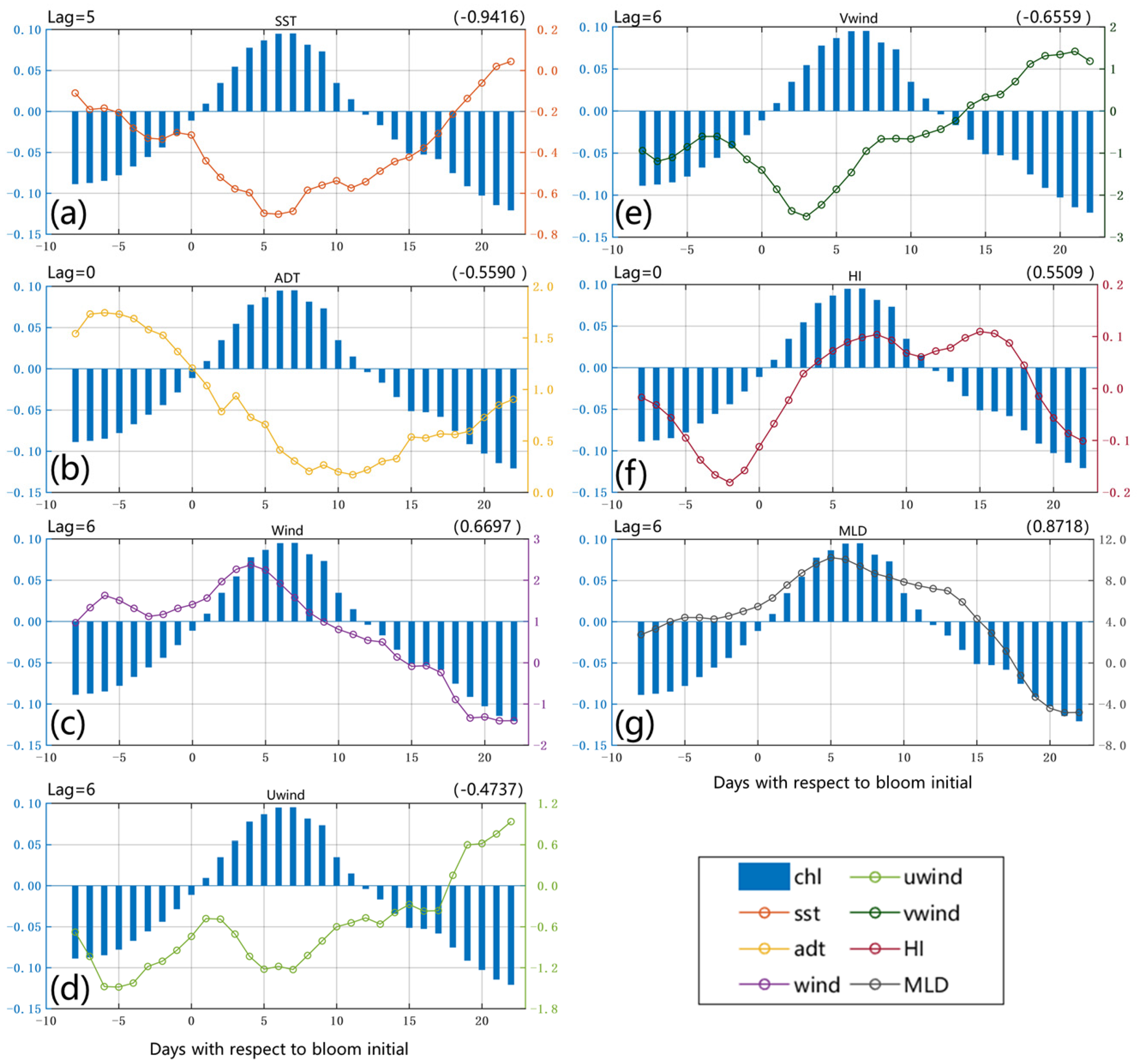
4. Controlling Factors

In this section, we focus on the analysis of the linkage between the occurrence of LZB events and the controlling factors, including SST, ADT, winds, HI, and MLD. Using the method detailed in Section 2.3, the composite of all the LZB events was achieved by temporally matching the onset (initial) day of each bloom as the first day of the x-axis (e.g., day 10 refers to 9 days after the initial day of a bloom event; Figure 9). For the normalized LZB event, a lag correlation was then applied from day −8 through day 22 (31-day). In Figure 9, the optimal lags for the controlling factors are different, which are six days for the wind and MLD, five days for ADT, and zero days for HI. There are unsurprisingly negative correlations for SST and ADT, in accordance with the textbook scenario of the upwelling of cold and nutrient-replete water. The wind speed (Figure 9c) and MLD (Figure 9g) led to the bloom for six days with a correlation coefficient of ~0.67 and ~0.87. The lag was likely due to the response time of phytoplankton to the wind-induced mixing and the associated MLD deepening. For the HI, as previously revealed by Guo et al. [9] the CHL high had a high correlation with the intensity of SST fronts.
We further analyze the bloom precursor composite (Figure 10a) and bloom peak composite (Figure 10b) to compare the environmental condition for the blooms. The bloom precursor is defined as the five-day average before the bloom, while the bloom peak is defined as the five-day window central at the peak day. For the offshore core of LZB (red circle in Figure 1a), a discernable co-location of CHL high and SST low is apparent, suggesting a direct link between LZB and the upwelling. Consistent with the lagged response of CHL to SST (Figure 9), the SST is coolest before the bloom, which is the responding time of the phytoplankton growth to the upwelling nutrients. The SSH presents a southwest-northeast-direction ADT high. The mismatch of a low-ADT and low-SST core implies that the eddy pumping [49] might not be the controlling mechanism for the bloom.
The most striking feature appears in the contrast between the two phases in the winds and the HI. The wind intensified before the bloom, with a maxima wind jet (>4.0 m s−1 anomaly) south of the bloom. Compared with the mean winter monsoon of 10 m s−1 (Figure 1c), this ~40% intensification is rather strong and can induce MLD deepening (Figure 10(a6)) and nutrient entrainments [5,6]. During the bloom peak, however, the wind shows very weak anomaly signals (i.e., wind relaxation). This suggests that the cycle of wind intensification and follow-on relaxation is important for the LZB. As we previously showed with a process-oriented modeling investigation [5], during the intensification, the mixed-layer entrainments contributed to the nutrient repletion to the euphotic zone, while the follow-on relaxation provided a stable water column for the phytoplankton to flourish [50]. On the other hand, HI showed hotspots of submesoscale frontal activity to the south of LZB during the bloom precursor days. For other offshore regions, the HI presents extremely low values outside of the Luzon Strait. In contrast, for the bloom peaking period, the HI presents systematic higher values in the whole domain. The distribution of the SST fronts is very similar to that of HI. In summary, the higher values for HI are scattered with shorter-scale filaments, implying the occurrence of submesoscale processes.
Dynamically, these features can be explained by the mixed-layer instability (MLI). MLI is a category of baroclinic instabilities that occur in the mixed-layer at submesoscales [51]. MLI can spontaneously happen from the mixed-layer with the lateral density gradient [52], such as the case for the bloom precursor period. The occurrence of MLI then drives the re-stratification of the mixed layer, providing a stable water column for the phytoplankton growth. The expression of MLI is much quicker than the mesoscale baroclinic instabilities [51]; thus, the phytoplankton can flourish earlier [17,53]. In numerical experiments comparing cases with and without MLI, blooms in the case with MLI can occur ~4 days earlier with a more intensive peak (~36%). The MLI is then expressed as small-scale eddies and filaments like those in the bloom peak (Figure 10(b5)). In summary, the winter monsoon intensification is vital for the nutrient supply of winter LZB, but both the relaxation and submesoscale processes are also essential conditions for the abnormally strong blooms.

5. Conclusions

In this study, we applied a new statistical framework [37]—the framework that has been widely utilized to study marine heatwaves—to define bloom events that frequently occur in the winter in the adjacent Luzon Strait (LZB) in the northeastern South China Sea (SCS). Especially, we make full use of a previously reconstructed remote sensing CHL dataset, the SCSDCT data, to study the LZB events from 2005 to 2019. With the framework, a total of 12 LZB events were defined. Each event was quantified with a series of statistical matrices, i.e., duration days, maximum intensity, mean intensity, and cumulated intensity. The LZB events persisted for 9.8 days on average, with a mean peak intensity of 0.27 mg m−3. The strongest event in the winter of 2014 was presented as an extreme case. Interestingly, the LZB presented a long-term trend towards fewer but stronger events, which can probably be linked to SST warming and other climate changes. We also analyzed the link of LZB events to controlling factors, i.e., SST, sea-surface height, winds, and two indexes derived from SST to quantify submesoscale activity. The lagged correlation suggested that submesoscale activity was also a statistically significant factor linked to the LZB. During the relaxation of the intensified winter monsoon, submesoscale baroclinic instabilities developed, leading to rapid stratification (and, hence, earlier and stronger blooms) and scattered submesoscale fronts. For the first time, this study systematically extracted the LZB events with remote sensing data by the novel use of a statistic framework. As well, this study highlighted the linkage of these bloom events to submesoscale activity. This linkage has been proposed in other oceans but has seldom been investigated for the SCS.
This application of this framework can provide a new perspective to studying the marine ecosystem. Indeed, compared with marine heatwaves, which are better understood and to which more attention is paid, the extreme events of phytoplankton bloom in the global ocean [54,55,56] were seldom, or even never, analyzed with this framework, partly because of the gapping nature of optic remote sensing. A lot of issues need to be addressed, such as (1) the contribution of bloom events to the ecosystem functions such as carbon pumping; (2) the response of bloom events to climate change. At the current point, using reconstructed data (as in this study) or reanalyzed ecosystem models (such as the NEMO-PISCES product [57]) can be a feasible solution to this issue. Numerical models should also be applied to fully understand the genesis and environmental effects of the bloom [58,59,60]. Moreover, CHL is an essential climate variable but is not the only variable that can be analyzed with this framework. After all, CHL, as a bio-optical variable, only reflects one single aspect of the marine ecosystem. Applications on, for instance, oxygen or carbonate system variables can be exploited in the future. The compound effects from multiple types of marine extremes (such as the MHW) are also an important topic that should be considered [39].

Author Contributions

Conceptualization, W.L. and X.G.; methodology, W.L. and X.G.; software, X.G.; validation, X.G. and S.L.; formal analysis, X.G., S.L., W.L. and Z.W.; investigation, S.L., W.L. and Z.W.; resources, X.G.; data curation, X.G. and T.W.; writing—original draft preparation, X.G.; writing—review and editing, W.L.; visualization, X.G.; supervision, Z.L.; project administration, C.X. and Z.L.; funding acquisition, W.L. All authors have read and agreed to the published version of the manuscript.

Funding

This research was funded by the National Natural Science Foundation of China (grant number 41906019).

Data Availability Statement

The SCSDCT CHL data presented in this study are openly available in Science Data Bank at https://doi.org/10.11922/sciencedb.01066, accessed on 1 May 2022.

Conflicts of Interest

The authors declare no conflict of interest.

References

  1. Wong, G.T.F.; Ku, T.L.; Mulholland, M.; Tseng, C.M.; Wang, D.P. The SouthEast Asian time-series study (SEATS) and the biogeochemistry of the South China Sea—An overview. Deep Sea Res. Part II Top. Stud. Oceanogr. 2007, 54, 1434–1447. [Google Scholar] [CrossRef]
  2. Lu, W.; Yan, X.-H.; Han, L.; Jiang, Y. One-dimensional ocean model with three types of vertical velocities: A case study in the South China Sea. Ocean. Dyn. 2017, 67, 253–262. [Google Scholar] [CrossRef]
  3. Tang, D.; Ni, I.-H.; Kester, D.R.; Muller-Karger, F.E. Remote sensing observations of winter phytoplankton blooms southwest of the Luzon Strait in the South China Sea. Mar. Ecol. Prog. Ser. 1999, 191, 43–51. [Google Scholar] [CrossRef] [Green Version]
  4. Shang, S.; Li, L.; Li, J.; Li, Y.; Lin, G.; Sun, J. Phytoplankton bloom during the northeast monsoon in the Luzon Strait bordering the Kuroshio. Remote Sens. Environ. 2012, 124, 38–48. [Google Scholar] [CrossRef]
  5. Lu, W.; Yan, X.-H.; Jiang, Y. Winter bloom and associated upwelling northwest of the Luzon Island: A coupled physical-biological modeling approach. J. Geophys. Res. Ocean. 2015, 120, 533–546. [Google Scholar] [CrossRef]
  6. Wang, J.; Tang, D.; Sui, Y. Winter phytoplankton bloom induced by subsurface upwelling and mixed layer entrainment southwest of Luzon Strait. J. Mar. Syst. 2010, 83, 141–149. [Google Scholar] [CrossRef]
  7. Xing, X.; Qiu, G.; Boss, E.; Wang, H. Temporal and Vertical Variations of Particulate and Dissolved Optical Properties in the South China Sea. J. Geophys. Res. Ocean. 2019, 124, 3779–3795. [Google Scholar] [CrossRef] [Green Version]
  8. Liu, H.; Liu, X.; Xiao, W.; Laws, E.A.; Huang, B. Spatial and temporal variations of satellite-derived phytoplankton size classes using a three-component model bridged with temperature in Marginal Seas of the Western Pacific Ocean. Prog. Oceanogr. 2021, 191, 102511. [Google Scholar] [CrossRef]
  9. Guo, L.; Xiu, P.; Chai, F.; Xue, H.; Wang, D.; Sun, J. Enhanced chlorophyll concentrations induced by Kuroshio intrusion fronts in the northern South China Sea. Geophys. Res. Lett. 2017, 44, 11565–11572. [Google Scholar] [CrossRef] [Green Version]
  10. Shuai, Y.; Li, Q.P.; Wu, Z. Biogeochemical Responses to Nutrient Fluxes in the Open South China Sea: A 3-D Modeling Study. J. Geophys. Res. Ocean. 2021, 126, e2020JC016895. [Google Scholar] [CrossRef]
  11. Gao, H.; Zhao, H.; Han, G.; Dong, C. Spatio-Temporal Variations of Winter Phytoplankton Blooms Northwest of the Luzon Island in the South China Sea. Front. Mar. Sci. 2021, 8, 637499. [Google Scholar] [CrossRef]
  12. Du, C.; Liu, Z.; Kao, S.J.; Dai, M. Diapycnal Fluxes of Nutrients in an Oligotrophic Oceanic Regime: The South China Sea. Geophys. Res. Lett. 2017, 44, 11510–11518. [Google Scholar] [CrossRef]
  13. Mahadevan, A. The Impact of Submesoscale Physics on Primary Productivity of Plankton. Ann. Rev. Mar. Sci. 2016, 8, 161–184. [Google Scholar] [CrossRef] [Green Version]
  14. Omand, M.M.; D’Asaro, E.A.; Lee, C.M.; Perry, M.J.; Briggs, N.; Cetinić, I.; Mahadevan, A. Eddy-driven subduction exports particulate organic carbon from the spring bloom. Science 2015, 348, 222–225. [Google Scholar] [CrossRef] [Green Version]
  15. McWilliams, J.C. Submesoscale, coherent vortices in the ocean. Rev. Geophys. 1985, 23, 165–182. [Google Scholar] [CrossRef]
  16. Molemaker, M.J.; McWilliams, J.C.; Yavneh, I. Baroclinic instability and loss of balance. J. Phys. Oceanogr. 2005, 35, 1505–1517. [Google Scholar] [CrossRef] [Green Version]
  17. Mahadevan, A.; D’Asaro, E.; Lee, C.; Perry, M.J. Eddy-driven stratification initiates North Atlantic spring phytoplankton blooms. Science 2012, 337, 54–58. [Google Scholar] [CrossRef]
  18. Dong, J.; Zhong, Y. The spatiotemporal features of submesoscale processes in the northeastern South China Sea. Acta Oceanol. Sin. 2018, 37, 8–18. [Google Scholar] [CrossRef]
  19. Lin, H.; Liu, Z.; Hu, J.; Menemenlis, D.; Huang, Y. Characterizing meso-to submesoscale features in the South China Sea. Prog. Oceanogr. 2020, 188, 102420. [Google Scholar] [CrossRef]
  20. Zhang, Z.; Zhang, X.; Qiu, B.; Zhao, W.; Zhou, C.; Huang, X.; Tian, J. Submesoscale Currents in the Subtropical Upper Ocean Observed by Long-Term High-Resolution Mooring Arrays. J. Phys. Oceanogr. 2021, 51, 187–206. [Google Scholar] [CrossRef]
  21. Zhong, Y.; Bracco, A.; Tian, J.; Dong, J.; Zhao, W.; Zhang, Z. Observed and simulated submesoscale vertical pump of an anticyclonic eddy in the South China Sea. Sci. Rep. 2017, 7, 44011. [Google Scholar] [CrossRef] [PubMed]
  22. Bagniewski, W.; Fennel, K.; Perry, M.J.; D’Asaro, E.A. Optimizing models of the North Atlantic spring bloom using physical, chemical and bio-optical observations from a Lagrangian float. Biogeosciences 2011, 8, 1291–1307. [Google Scholar] [CrossRef] [Green Version]
  23. Kuroda, H.; Takasuka, A.; Hirota, Y.; Kodama, T.; Ichikawa, T.; Takahashi, D.; Aoki, K.; Setou, T. Numerical experiments based on a coupled physical–biochemical ocean model to study the Kuroshio-induced nutrient supply on the shelf-slope region off the southwestern coast of Japan. J. Mar. Syst. 2018, 179, 38–54. [Google Scholar] [CrossRef]
  24. Lévy, M.; Iovino, D.; Resplandy, L.; Klein, P.; Madec, G.; Tréguier, A.M.; Masson, S.; Takahashi, K. Large-scale impacts of submesoscale dynamics on phytoplankton: Local and remote effects. Ocean. Model. 2012, 43, 77–93. [Google Scholar] [CrossRef]
  25. Lévy, M.; Klein, P.; Treguier, A.-M. Impact of sub-mesoscale physics on production and subduction of phytoplankton in an oligotrophic regime. J. Mar. Res. 2001, 59, 535–565. [Google Scholar] [CrossRef] [Green Version]
  26. Lévy, M.; Resplandy, L.; Lengaigne, M. Oceanic mesoscale turbulence drives large biogeochemical interannual variability at middle and high latitudes. Geophys. Res. Lett. 2014, 41, 2467–2474. [Google Scholar] [CrossRef]
  27. Mahadevan, A.; Archer, D. Modeling the impact of fronts and mesoscale circulation on the nutrient supply and biogeochemistry of the upper ocean. J. Geophys. Res. Ocean. 2000, 105, 1209–1225. [Google Scholar] [CrossRef] [Green Version]
  28. Castro, S.L.; Emery, W.J.; Wick, G.A.; Tandy, W. Submesoscale Sea Surface Temperature Variability from UAV and Satellite Measurements. Remote Sens. 2017, 9, 1089. [Google Scholar] [CrossRef] [Green Version]
  29. Gaube, P.; Chickadel, C.C.; Branch, R.; Jessup, A. Satellite Observations of SST-Induced Wind Speed Perturbation at the Oceanic Submesoscale. Geophys. Res. Lett. 2019, 46, 2690–2695. [Google Scholar] [CrossRef]
  30. Hosegood, P.J.; Nightingale, P.D.; Rees, A.P.; Widdicombe, C.E.; Woodward, E.M.S.; Clark, D.R.; Torres, R.J. Nutrient pumping by submesoscale circulations in the mauritanian upwelling system. Prog. Oceanogr. 2017, 159, 223–236. [Google Scholar] [CrossRef] [Green Version]
  31. Liu, X.; Levine, N.M. Enhancement of phytoplankton chlorophyll by submesoscale frontal dynamics in the North Pacific Subtropical Gyre. Geophys. Res. Lett. 2016, 43, 1651–1659. [Google Scholar] [CrossRef] [PubMed]
  32. Ni, Q.; Zhai, X.; Wilson, C.; Chen, C.; Chen, D. Submesoscale Eddies in the South China Sea. Geophys. Res. Lett. 2021, 48, e2020GL091555. [Google Scholar] [CrossRef]
  33. Xu, G.; Yang, J.; Dong, C.; Chen, D.; Wang, J. Statistical study of submesoscale eddies identified from synthetic aperture radar images in the Luzon Strait and adjacent seas. Int. J. Remote Sens. 2015, 36, 4621–4631. [Google Scholar] [CrossRef]
  34. Hobday, A.J.; Alexander, L.V.; Perkins, S.E.; Smale, D.A.; Straub, S.C.; Oliver, E.C.J.; Benthuysen, J.A.; Burrows, M.T.; Donat, M.G.; Feng, M.; et al. A hierarchical approach to defining marine heatwaves. Prog. Oceanogr. 2016, 141, 227–238. [Google Scholar] [CrossRef] [Green Version]
  35. Oliver, E.C.J. Mean warming not variability drives marine heatwave trends. Clim. Dyn. 2019, 53, 1653–1659. [Google Scholar] [CrossRef]
  36. Oliver, E.C.J.; Donat, M.G.; Burrows, M.T.; Moore, P.J.; Smale, D.A.; Alexander, L.V.; Benthuysen, J.A.; Feng, M.; Sen Gupta, A.; Hobday, A.J.; et al. Longer and more frequent marine heatwaves over the past century. Nat. Commun. 2018, 9, 1324. [Google Scholar] [CrossRef]
  37. Oliver, E.C.J.; Benthuysen, J.A.; Darmaraki, S.; Donat, M.G.; Hobday, A.J.; Holbrook, N.J.; Schlegel, R.W.; Sen Gupta, A. Marine Heatwaves. Ann. Rev. Mar. Sci. 2021, 13, 313–342. [Google Scholar] [CrossRef]
  38. Lindstrom, E.; Gunn, J.; Fischer, A.; McCurdy, A.; Glover, L.K. A Framework for Ocean Observing. By the Task Team for an Integrated Framework for Sustained Ocean Observing; Unesco: Paris, France, 2012. [Google Scholar]
  39. Gruber, N.; Boyd, P.W.; Frolicher, T.L.; Vogt, M. Biogeochemical extremes and compound events in the ocean. Nature 2021, 600, 395–407. [Google Scholar] [CrossRef]
  40. Boyce, D.G.; Lewis, M.R.; Worm, B. Global phytoplankton decline over the past century. Nature 2010, 466, 591–596. [Google Scholar] [CrossRef]
  41. Oey, L.Y.; Chang, M.C.; Huang, S.M.; Lin, Y.C.; Lee, M.A. The influence of shelf-sea fronts on winter monsoon over East China Sea. Clim. Dyn. 2015, 45, 2047–2068. [Google Scholar] [CrossRef]
  42. Wang, T.; Yu, P.; Wu, Z.; Lu, W.; Liu, X.; Li, Q.P.; Huang, B. Revisiting the Intraseasonal Variability of Chlorophyll-a in the Adjacent Luzon Strait With a New Gap-Filled Remote Sensing Data Set. IEEE Trans. Geosci. Remote Sens. 2021, 60, 1–11. [Google Scholar] [CrossRef]
  43. Xiao, W.; Wang, L.; Laws, E.; Xie, Y.; Chen, J.; Liu, X.; Chen, B.; Huang, B. Realized niches explain spatial gradients in seasonal abundance of phytoplankton groups in the South China Sea. Prog. Oceanogr. 2018, 162, 223–239. [Google Scholar] [CrossRef]
  44. Belkin, I.M.; O’Reilly, J.E. An algorithm for oceanic front detection in chlorophyll and SST satellite imagery. J. Mar. Syst. 2009, 78, 319–326. [Google Scholar] [CrossRef]
  45. Chin, T.M.; Vazquez-Cuervo, J.; Armstrong, E.M. A multi-scale high-resolution analysis of global sea surface temperature. Remote Sens. Environ. 2017, 200, 154–169. [Google Scholar] [CrossRef]
  46. Hersbach, H.; Bell, B.; Berrisford, P.; Hirahara, S.; Horányi, A.; Muñoz-Sabater, J.; Nicolas, J.; Peubey, C.; Radu, R.; Schepers, D.; et al. The ERA5 global reanalysis. Q. J. R. Meteorol. Soc. 2020, 146, 1999–2049. [Google Scholar] [CrossRef]
  47. Thomson, R.E.; Emery, W.J. Data Analysis Methods in Physical Oceanography; Newnes: Oxford, UK, 2014. [Google Scholar]
  48. Sen, P.K. Estimates of the regression coefficient based on Kendall’s tau. J. Am. Stat. Assoc. 1968, 63, 1379–1389. [Google Scholar] [CrossRef]
  49. Chen, Y.-L.L.; Chen, H.-Y.; Lin, I.-I.; Lee, M.-A.; Chang, J. Effects of cold eddy on phytoplankton production and assemblages in Luzon Strait bordering the South China Sea. J. Oceanogr. 2007, 63, 671–683. [Google Scholar] [CrossRef]
  50. Sverdrup, H.U. On conditions for the vernal blooming of phytoplankton. ICES J. Mar. Sci. 1953, 18, 287–295. [Google Scholar] [CrossRef]
  51. Boccaletti, G.; Ferrari, R.; Fox-Kemper, B. Mixed Layer Instabilities and Restratification. J. Phys. Oceanogr. 2007, 37, 2228–2250. [Google Scholar] [CrossRef]
  52. Fox-Kemper, B.; Ferrari, R.; Hallberg, R. Parameterization of Mixed Layer Eddies. Part I: Theory and Diagnosis. J. Phys. Oceanogr. 2008, 38, 1145–1165. [Google Scholar] [CrossRef]
  53. Taylor, J.R.; Ferrari, R. Ocean fronts trigger high latitude phytoplankton blooms. Geophys. Res. Lett. 2011, 38, L23601. [Google Scholar] [CrossRef]
  54. Bondur, V.G.; Zamshin, V.V.; Chvertkova, O.I. Space Study of a Red Tide-Related Environmental Disaster near Kamchatka Peninsula in September–October 2020. Dokl. Earth Sci. 2021, 497, 255–260. [Google Scholar] [CrossRef]
  55. Yagci, A.L.; Colkesen, I.; Kavzoglu, T.; Sefercik, U.G. Daily monitoring of marine mucilage using the MODIS products: A case study of 2021 mucilage bloom in the Sea of Marmara, Turkey. Environ. Monit. Assess. 2022, 194, 170. [Google Scholar] [CrossRef] [PubMed]
  56. Wei, G.; Tang, D.; Wang, S. Distribution of chlorophyll and harmful algal blooms (HABs): A review on space based studies in the coastal environments of Chinese marginal seas. Adv. Space Res. 2008, 41, 12–19. [Google Scholar] [CrossRef]
  57. Aumont, O.; Éthé, C.; Tagliabue, A.; Bopp, L.; Gehlen, M. PISCES-v2: An ocean biogeochemical model for carbon and ecosystem studies. Geosci. Model Dev. 2015, 8, 2465–2513. [Google Scholar] [CrossRef] [Green Version]
  58. Lu, W.; Wang, J.; Jiang, Y.; Chen, Z.; Wu, W.; Yang, L.; Liu, Y. Data-Driven Method with Numerical Model: A Combining Framework for Predicting Subtropical River Plumes. J. Geophys. Res. Ocean. 2022, 127, e2021JC017925. [Google Scholar] [CrossRef]
  59. Lu, W.; Oey, L.-Y.; Liao, E.; Zhuang, W.; Yan, X.-H.; Jiang, Y. Physical modulation to the biological productivity in the summer Vietnam upwelling system. Ocean. Sci. 2018, 14, 1303–1320. [Google Scholar] [CrossRef] [Green Version]
  60. Lu, W.; Luo, Y.; Yan, X.; Jiang, Y. Modeling the Contribution of the Microbial Carbon Pump to Carbon Sequestration in the South China Sea. Sci. China Earth Sci. 2018, 61, 1594–1604. [Google Scholar] [CrossRef]
Figure 1. Winter-average (a) CHL (mg m−3), (b) sea surface temperature (degree Celsius), (c) absolute dynamic topography (cm), (d) winds (color for speed in m s−1 corresponding wind vectors), (e) heterogeneity index, (f) sea surface temperature fronts (°C km−1), and (g) mixed-layer depth (m). In (a), the black box indicates the zoom-in region, while the white box indicates the regions of the winter Luzon Bloom. The red circle outlines the rough position of the offshore wing of the Luzon Bloom (see text). In (bg), the white boxes indicate the region of average taken for the driving factors for the following analysis. Winter here is defined as November through February, while the timespan for the average is 2005–2019.
Remotesensing 14 03557 g001
Figure 2. Illustration of the marine bloom event definition (H16 framework). The black line indicates the time series of CHL, while the blue line is the daily climatology of CHL. The defined threshold (green line, 90th percentile in this case) is changing with the day of the year. When the CHL concentration exceeds this threshold for more than 5 days, a bloom event is defined with a corresponding start date, end date, peak date, duration, and peak intensity. See the text for a detailed explanation.
Remotesensing 14 03557 g002
Figure 3. Time series of Box-A averaged SCSDCT CHL concentration (black), the threshold of the 90th percentile (green), and the climatological mean (blue). Red shading indicates the winter periods (November through February). Arrows indicate the 12 identified LZB events.
Remotesensing 14 03557 g003
Figure 4. The indicators of extracted LZB events (in CHL anomalies with respect to 365-day climatology), showing the (a) duration in days, (b) maximum intensity in mg m−3, (c) cumulative intensity in mg m−3 d, and (d) mean intensity in mg m−3. The definition of these indicators is shown in Section 2.2. Each bar corresponds to a bloom event, while red bars highlight the strongest event of the 2014 winter. The x-axis position of each bar indicates the time of occurrence.
Remotesensing 14 03557 g004
Figure 5. Daily CHL anomaly (relative to the daily climatology, unit: mg m−3) for the Jan 2014 bloom event. (af) are for different date.
Remotesensing 14 03557 g005
Figure 6. Daily anomalies of SST (color shading) and SSH (contours) relative to the corresponding climatology for the Jan 2014 bloom event. (af) are for different date.
Remotesensing 14 03557 g006
Figure 7. The 15-year trends of (a) mean bloom intensity (mg m−3 per year), (b) maximum intensity (mg m−3 per year), (c) annual cumulative intensity (mg m−3 days per year), and (d) mean duration (days per year). The trends with p > 0.1 were masked with gray stipples.
Remotesensing 14 03557 g007
Figure 8. Histogram of the pixelwise CHL anomaly at all points of the small box in Figure 1a in 2005–2010 (green) and 2014–2019 (pink). The CHL anomaly is with respect to the 365-day climatology. The red line shows the thresholds of 90th percentile averaged from all thresholds in the domain.
Remotesensing 14 03557 g008
Figure 9. The composite anomaly of LZB events and the corresponding controlling factor, including (a) SST, (b) ADT, (c) wind speed, (d) the u-component of wind, (e) the v-component of wind, (f) HI, and (g) MLD. The anomaly means removing the climatology of each factor. The x-axis is in days with respect to the bloom initials (e.g., −5 refers to five days before each bloom event). All factors and CHL were the averages of all 12 bloom events, with the maximum-correlated lag and correlation coefficients listed above each panel. For the winds and HI, a five-day moving average window was applied to the data to filter high-frequency fluctuations. All the correlations are significant at the 99% level.
Remotesensing 14 03557 g009
Figure 10. Composite of the five-day average of the (a) precursor and (b) peak of LZB bloom events according to LZB area-averaged CHL, including CHL (a1,b1), SST (a2,b2), ADT (a3,b3), wind speed with wind vectors (a4,b4), HI (a5,b5), and MLD (a6,b6). The distribution of SST fronts is similar to that of HI, which is not shown here.
Remotesensing 14 03557 g010
Table 1. Summary of the remote sensing datasets in this study.
Data AbbreviationVariableFull NameSource *ReferencesResolution
SCSDCTCHLSouth China Sea Full-coverage Daily 4 km Surface Chlorophyll-a Remote Sensing Reconstruction Dataset from Discrete Cosine Transform 2005–2019https://www.scidb.cn/detail?dataSetId=1387ffe83af54f0fb574d60e97b206b2[42]4 km × 4 km
MURSST and HI and frontal intensity derived from SSTMulti-scale Ultra-high Resolution (MUR) Sea Surface Temperaturehttps://podaac.jpl.nasa.gov/MEaSUREs-MUR?sections=data[31,44,45]0.01° × 0.01°
ERA5Meridional and zonal windFifth generation of the European Center
for Medium-Range Weather Forecasts atmospheric reanalyses of the global climate
https://cds.climate.copernicus.eu/cdsapp#!/dataset/reanalysis-era5-single-levels?tab=overview[46]0.1° × 0.1°
AVISOSSH and Absolute Dynamic Topography (ADT)Archiving, Validation, and Interpretation of Satellite Oceanographichttps://resources.marine.copernicus.eu/?option=com_csw&view=details&product_id=SEALEVELGLO_PHY_L4_REP_OBSERVATIONS_008_047/0.25° × 0.25°
GLORYSMixed-Layer Depth (MLD) Mixed-layer depth from the GLORYSV12 reanalysis product from the Copernicus Marine Servicehttps://resources.marine.copernicus.eu/product-detail/GLOBAL_MULTIYEAR_PHY_001_030/INFORMATION/0.083° × 0.083°
* All links were last accessed on 1 May 2022.
Publisher’s Note: MDPI stays neutral with regard to jurisdictional claims in published maps and institutional affiliations.

