A Superpixel Spatial Intuitionistic Fuzzy C-Means Clustering Algorithm for Unsupervised Classification of High Spatial Resolution Remote Sensing Images

Abstract

This paper proposes a superpixel spatial intuitionistic fuzzy C-means (SSIFCM) clustering algorithm to address the problems of misclassification, salt and pepper noise, and classification uncertainty arising in the pixel-level unsupervised classification of high spatial resolution remote sensing (HSRRS) images. To reduce information redundancy and ensure noise immunity and image detail preservation, we first use a superpixel segmentation to obtain the local spatial information of the HSRRS image. Secondly, based on the bias-corrected fuzzy C-means (BCFCM) clustering algorithm, the superpixel spatial intuitionistic fuzzy membership matrix is constructed by counting an intuitionistic fuzzy set and spatial function. Finally, to minimize the classification uncertainty, the local relation between adjacent superpixels is used to obtain the classification results according to the spectral features of superpixels. Four HSRRS images of different scenes in the aerial image dataset (AID) are selected to analyze the classification performance, and fifteen main existing unsupervised classification algorithms are used to make inter-comparisons with the proposed SSIFCM algorithm. The results show that the overall accuracy and Kappa coefficients obtained by the proposed SSIFCM algorithm are the best within the inter-comparison of fifteen algorithms, which indicates that the SSIFCM algorithm can effectively improve the classification accuracy of HSRRS image.

1. Introduction

With the vigorous development of earth observation technology, high spatial resolution remote sensing (HSRRS) images are widely used in many fields, such as disaster monitoring, agricultural management, urban and rural planning, as well as national defense construction [1]. Image classification is the basis of computer interpretation, a key step to complete information extraction, data mining, and resource integration. Whether the classification results are accurate plays a vital role in the qualitative and quantitative analysis of images, and the same function in the effective extraction and utilization of thematic information [2]. However, the problems of “same objects with different spectra” and “different objects with the same spectrum” are widespread and bring significant challenges to the accurate classification of HSRRS images.

The essence of classification is to classify each pixel or object in the image into different categories according to certain rules based on its spectral characteristics, spatial structure characteristics, or other information in different spectral bands. Generally, HSRRS image classification can be divided into supervised and unsupervised classification. Generally speaking, supervised classification results are greatly affected by human subjectivity, and poor recognition of undefined or too few categories, in practical applications. In contrast, unsupervised classification does not require prior category knowledge to build a discriminant function; based on specific algorithms and the concept of similarity, pixels with similar features are clustered. Thus, it is more popular and widely applied [3]. However, traditional unsupervised classification algorithms, such as K-means and the iterative self-organizing data analysis technique algorithm (ISODATA), are both ‘hard’ clustering algorithms with a single classification basis. Hence the resulting categories are so difficult to control that the algorithms can easily fall into local optima and have classification uncertainties. The proposed classification method, based on fuzzy mathematics theory, has good results in solving the problem of HSRRS image classification uncertainty. For example, the fuzzy C-means clustering (FCM) algorithm considers the fuzzy characteristics between samples and classes in the membership degree, and completes the automatic classification by optimizing the objective function to obtain the membership degree [4]. FCM is better than hard clustering because it has higher tolerance for fuzziness and can retain more original image information. However, FCM is sensitive to noise and the function convergence is slow. Furthermore, a classification based on a single membership degree is not sufficient to describe the fuzzy information of the image, which cannot completely solve the problem of classification uncertainty.

To overcome the shortcomings of the FCM algorithm, scholars around the world carried out a large number of studies, mainly forming three improved methods: (1) Spatial neighborhood information is introduced into the objective function to suppress the influence of abnormal data on clustering results [5,6]. However, introducing local spatial information is similar to pre-image filtering [7], which often increases computational complexity. (2) Replacing Euclidean distance with kernel distance to solve the initial clustering sensitivity problem of objective function [8,9], but the applicability of kernel distance for complex images clustering needs to be improved. (3) Modify the membership function and add specific parameters to balance the limitations of single membership clustering classification [10,11]. Although the classification effect is improved, the uncertainty is not entirely solved. To solve this problem, Xu et al. [12] proposed an intuitionistic FCM (IFCM) clustering algorithm based on FCM and intuitionistic fuzzy set (IFS). Relevant researches [13,14] applied IFS into HSRRS image change detection and image segmentation and uncertainty problem in the clustering process is well resolved. However, IFCM with pixels as the basic unit only considers the spectral information of pixels and ignores the spatial characteristics of images, so it cannot denoise the salt and pepper noises.

Ren et al. [15] first proposed the concept of superpixels and applied it to image segmentation in 2003. Preprocessing by using superpixel segmentation can effectively extract local features and express image structure information, reducing the salt and pepper noise of classification, and effectively, the computational complexity of unsupervised classification [16]. In recent years, numerous scholars turned their attention to the study of unsupervised classification methods that combine superpixels and FCM algorithms. The performance of the FCM algorithm is improved by introducing local spatial information with superpixels. The superpixel-based fast FCM (SFFCM) clustering algorithm [17] and the fast and robust FCM (FRFCM) clustering algorithm [18] change the traditional unsupervised classification from the pixel level to the object level, which improves robustness while reducing the complexity of the algorithm. However, both algorithms only consider membership degree as the basis for classification, which is prone to misclassification in practical applications due to the influence of classification uncertainty. The researchers improved the FCM by combining superpixels, but the discriminability of images with spectral heterogeneity was lower [19,20]. Other scholars paid attention to HSRRS image superpixel segmentation [21,22] and realized adaptive determination of the segmentation scale and provided good support for subsequent classification. The object-level unsupervised classification method, combined with the superpixel and FCM algorithm, has better classification performance, which provides conditions for the homogeneous region clustering of images by comprehensive utilization of spectral and spatial information.

In summary, a superpixel spatial intuitionistic fuzzy C-means (SSIFCM) clustering algorithm for the object-level unsupervised classification of HSRRS images is proposed in this paper. IFS theory is introduced to add a degree of uncertainty and non-membership into the FCM algorithm in order to solve the problem of classification uncertainty. Considering spatial neighborhood information and spatial function, the problem that adjacent pixels with similar feature intensity are easily classified into the same category can be solved. By introducing superpixels, the unsupervised classification of HSRRS images changes from the pixel level to the object level, the feature information of the object increases, the phenomenon of salt and pepper is solved, and finally, the accurate classification of HSRRS images is realized.

The contributions of this research consist of the following three aspects:

• We design an unsupervised classification algorithm of HSRRS images with superpixel spatial intuitionistic fuzzy C-means clustering, namely SSIFCM. By combining superpixel segmentation with a modified affiliation function to resolve classification uncertainty, it minimizes computing complexity and overcomes salt and pepper noise.
• Before applying the FCM algorithm, SSIFCM calculates an image’s local spatial information by superpixel segmentation, which decreases the computational complexity associated with introducing local spatial information to overcome noise. SSIFCM captures object-level features of a superpixel image, allowing full utilization of the image’s content while ensuring noise immunity.
• Based on the obtained superpixel image, a superpixel spatial intuitive fuzzy membership is constructed, this maximizes the robust decision-making interval, which enhances the accuracy of fuzzy clustering. Therefore, for information-rich HSRRS images, our proposed SSIFCM is more robust than the comparison algorithm.

The rest of this paper is organized as follows. Section 2 details the proposed algorithm. Followed by the description of the dataset, experiments and results in Section 3. The discussion is presented in Section 4. Finally, conclusions are drawn in Section 5.

2. Materials and Methods

To solve the problems of misclassification, salt and pepper noises, and classification uncertainty of pixel-level HSRRS image unsupervised classification, we propose the SSIFCM algorithm, which is divided into three steps: (1) The simple linear iterative clustering (SLIC) [23] algorithm is used to segment the preprocessed HSRRS image into superpixels. (2) Setting an appropriate threshold, we use the SSIFCM algorithm to unsupervised classify superpixel images according to their spectral features and local relationships. (3) Color space is used to assign values to categories, and the figure of the final classification result is obtained.

2.1. Superpixel Segmentation

Before fuzzy clustering, SSIFCM obtains local spatial information of HSRRS images by SLIC algorithm. The SLIC algorithm clusters based on the similarity of pixels in the image plane space, and the generated superpixels are compact, uniform, regular in shape, and easy to express neighborhood features. Compared with other algorithms, the SLIC algorithm is a simple idea: super-pixel segmentation based on the color and distance measurements of pixels can integrate the spectral and spatial characteristics of images, which is more suitable for the classification of HSRRS images of ground objects with complex details.

The main steps of calculating the local spatial information of HSRRS images are as follows:

(1)

Converting HSRRS images with N pixels from the RGB color space to the CIELab color space [24];

(2)

Define two features $C_j={\left[l_j,a_j,b_j\right]}^T$ and $S_j={\left[x_j,y_j\right]}^T$ in the CIELab color space of the image. $C_j$ and $S_j$ represent the color value and the planimetric position of the jth pixel, respectively. Where, $l_j$ represents the brightness in the Lab color model, $a_j$ and $b_j$ represent the channels from green to red and blue to yellow, respectively,$x_j$ and $y_j$ are the two-dimensional plane coordinates of the pixel j. First, the clustering center is initialized, then the k seed points are randomly and uniformly sampled in the image containing N pixels. The sampling interval is S:

$$S=\sqrt{\frac{N}{k}}$$

(1)

(3)

To avoid superpixels concentrating on image edges or noise pixels, the clustering center is moved to the corresponding position of the lowest gradient amplitude in the $3\times 3$ neighborhood. Finally, in the neighborhood around each seed point, the clustering center is marked for each pixel point according to the distance D:

$$D\left(j,g\right)=\sqrt{{\left(\frac{d_c}{N_C}\right)}^2+{\left(\frac{d_s}{N_S}\right)}^2}=\sqrt{{\left(\frac{\Vert C_j-C_g\Vert }{N_C}\right)}^2+{\left(\frac{\Vert S_j-S_g\Vert }{S}\right)}^2}$$

(2)

The distance D represents the tightness between the pixel and cluster center and is used to determine the segmentation area of the pixel. $d_c$ represents the color distance, $d_s$ represents the spatial distance, and g is the cluster center’s (superpixels) label. $N_c$ is the color normalization constant and denotes the maximum color distance. $N_c$ varies with different images and clusters and is generally replaced by a fixed value range from 1 to 40 (20 in this paper). $N_s$ is a space distance normalization constant that represents the maximum space distance within the class ($N_s=S$).

(4)

After iteration, the clustering center (superpixels) will be updated as the vector average, and the pixel values of the clustering center is:

$${\phi }_g=\frac{1}{{\gamma }_g}{\displaystyle \sum _{j\in G_g}\left[\begin{array}{l}{C}_j\\ S_j\end{array}\right]}$$

(3)

where $G_g$ represents the clustering of the center ${\phi }_g$(the g-th superpixel), ${\phi }_g$ is the average vector of $G_g$, ${\gamma }_g$ is the number of pixels in $G_g$. The iterative update is repeated until the preset number of iterations is reached (generally 10).

2.2. SSIFCM Clustering Algorithm

The traditional FCM does not consider the spatial neighborhood information of pixels in image classification and only uses the gray information of the image to calculate the membership degree. As a result, the noise pixels are easily misclassified due to abnormal feature information, which is only suitable for images with less noise. In order to classify HSRRS images using FCM, it is necessary to consider spatial neighborhood information in the clustering process. To compensate for the nonuniformity of traditional FCM, Ahmed et al. introduced a parameter α that allows pixels to be affected by their adjacent labels in the FCM objective function. He obtained the bias-corrected fuzzy C-means (BCFCM) algorithm [25] based on deviation correction. The objective function is as follows:

$$J_{BC}={\displaystyle \sum _{i=1}^C{\displaystyle \sum _{j=1}^N{u}_{ij}^m{\Vert z_j-v_i\Vert }^2}}+\frac{\alpha }{N_R}{\displaystyle \sum _{i=1}^C{\displaystyle \sum _{j=1}^N{u}_{ij}^m\left({\displaystyle \sum _{z_r\in N_j}{\Vert z_r-v_i\Vert }^2}\right)}}$$

(4)

where $z_j$ is the grayscale value the j-th pixel in the image, C represents the expected number of categories, N is the number of pixels in the given image,$u_{ij}^m$ is the membership of the j-th pixel belonging to the i-th category in the image, $v_i$ is the i-th clustering center, parameter m is a weighting exponent on each fuzzy membership and determines the amount of fuzziness of the resulting classification, parameter $\alpha$ controls the effects of the neighbor item, $N_j$ stands for the domain pixel in the surrounding window of $z_j$ and $N_R$ is the cardinality of $N_j$, $z_r$ is the neighborhood pixels in the window around pixel j, and $\Vert \Vert$ is a norm metric, which represents the Euclidean distance between the pixel and the clustering center denoting Euclidean distance between pixels and clustering centuries. $J_{BC}$ represents the sum of Euclidean distances from all pixels to each cluster center. FCM clustering is essentially finding the corresponding membership matrix and clustering center when the objective function J takes the minimum value.

BCFCM mainly calculates the membership degree of the sample points to the clustering center by optimizing the objective function, so as to judge the classification of the sample points. The pixels in the HSRRS image are the sample points of the data set in the BCFCM algorithm, and their characteristics (such as spectral characteristics) are sample characteristics. The algorithm is not sensitive to noise, but the introduction of spatial neighborhood information makes the distance between the pixels in the local neighborhood window and the clustering center repeat, which increases the computational complexity.

The introduction of superpixels achieves the preservation of spatial neighborhood information while effectively reducing the amount of computation. To reduce the number of pixels in the image, increase the feature information of the object, and improve the effectiveness of image classification and calculation efficiency, the SLIC algorithm is used to realize the pre-segmentation of the image, and the pixel value in the original image region is replaced by the spectral mean of the superpixel region.

In this paper, the input image is segmented by superpixel, and the superpixel region is regarded as the basic unit of subsequent classification. The statistical method of the regional CIELab color histogram is used to extract the spectral features of superpixels. Q superpixels are obtained in the HSRRS image, and the spectral mean ${\xi }_g\left(g=1,2,\dots ,Q\right)$ of each superpixel region is calculated to extract spectral features and encode the superpixel regions in the image. Finally, the Euclidean distance between the superpixels and each clustering center is calculated to complete clustering.

$${\xi }_g=\frac{1}{{\gamma }_g}{\displaystyle \sum _{j\in G_g}{C}_j}$$

(5)

where $G_g$ represents the clustering of the center ${\xi }_g$ (the g-th superpixel). After the completion of superpixel segmentation and spectral feature extraction, the uncertainty and spatial function are added to merge the superpixel segmentation regions based on BCFCM. The algorithm merges adjacent superpixels with similar attributes or features into a region according to the merging criterion. The objective function of the SSIFCM algorithm is:

$$J={\displaystyle \sum _{i=1}^C{\displaystyle \sum _{g=1}^Q{\gamma }_g{u}_{ig}^m{\Vert {\xi }_g-v_i\Vert }^2}}+\frac{\alpha }{N_R}{\displaystyle \sum _{i=1}^C{\displaystyle \sum _{g=1}^Q{u}_{ig}^m\left({\displaystyle \sum _{G_r\in N_g}{\gamma }_r{\Vert {\xi }_r-v_i\Vert }^2}\right)}}+{\pi }^{IFE}$$

(6)

$${\displaystyle \sum _{i=1}^C{u}_{ig}}=1$$

(7)

where ${\xi }_r$ represents the spectral mean of adjacent superpixels around superpixel $G_g$, $N_g$ stands for the set of neighboring superpixels that exist in a window around $G_g$ and $G_r$ is the neighborhood superpixels in the window around $G_g$, ${\gamma }_r$ is the number of pixels in superpixel $G_g$. ${\pi }^{IFE}$ represents intuitionistic fuzzy entropy (IFE) [26], which is considered to express the degree of fuzziness in the clusters. The IFE was introduced to maximise the valid data points in the clustering and minimise the entropy of the data matrix. When the uncertainty of the elements in each cluster is known, the corresponding IFE can be calculated. IFE is defined as:

$${\pi }^{IFE}={\displaystyle \sum _{i=1}^C{\pi }_i^{*}{e}^{\left(1-{\pi }_i^{*}\right)}}$$

(8)

$${\pi }_i^{*}=\frac{1}{Q}{\displaystyle \sum _{g=1}^Q{\pi }_{ig}}$$

(9)

where ${\pi }_{ig}$ is the uncertainty and represents the degree of hesitancy of superpixel $G_g$ to the ith cluster. The objective functions of the SSIFCM algorithm are as follows:

$$J={\displaystyle \sum _{i=1}^C{\displaystyle \sum _{g=1}^Q{\gamma }_g{u}_{ig}^m{\Vert {\xi }_g-v_i\Vert }^2}}+\frac{\alpha }{N_R}{\displaystyle \sum _{i=1}^C{\displaystyle \sum _{g=1}^Q{u}_{ig}^m\left({\displaystyle \sum _{G_r\in N_g}{\gamma }_r{\Vert {\xi }_r-v_i\Vert }^2}\right)}}+{\displaystyle \sum _{i=1}^C{\pi }_{ig}{e}^{\left(1-{\pi }_{ig}\right)}}$$

(10)

In this paper, the same method as traditional FCM is used to find the minimum value of the objective function, and iterative optimization is used to optimize the objective function. According to the Lagrange multiplier method, the following equation is constructed:

$$F={\displaystyle \sum _{i=1}^C{\displaystyle \sum _{g=1}^Q{\gamma }_g{u}_{ig}^m{\Vert {\xi }_g-v_i\Vert }^2}}+\frac{\alpha }{N_R}{\displaystyle \sum _{i=1}^C{\displaystyle \sum _{g=1}^N{u}_{ig}^m\left({\displaystyle \sum _{G_r\in N_g}{\gamma }_r{\Vert {\xi }_r-v_i\Vert }^2}\right)}}+{\displaystyle \sum _{i=1}^C{\pi }_i^{*}{e}^{\left(1-{\pi }_i^{*}\right)}}+{\displaystyle \sum _{g=1}^Q{\lambda }_g\left(1-{\displaystyle \sum _{i=1}^C{u}_{ig}}\right)}$$

(11)

Taking the derivatives of $u_{ig}$ and $v_i$, the equation is set to 0 to obtain the calculation formula of the superpixel fuzzy membership $u_{ig}$ and initial cluster center $v_i$ of the SSIFCM:

$$u_{ig}={\left[{\displaystyle \sum _{k=1}^C{\left[\frac{{\gamma }_g{\Vert {\xi }_g-v_i\Vert }^2+\frac{\alpha }{N_{ R}}{\displaystyle \sum _{G_r\in N_g}{\gamma }_r{\Vert {\xi }_r-v_i\Vert }^2}}{{\gamma }_g{\Vert {\xi }_g-v_k\Vert }^2+\frac{\alpha }{N_{ R}}{\displaystyle \sum _{G_r\in N_g}{\gamma }_r{\Vert {\xi }_r-v_k\Vert }^2}}\right]}^{\frac{1}{\left(m-1\right)}}}\right]}^{-1}$$

(12)

$$v_i=\left[{\displaystyle \sum _{g=1}^Q{u}_{ig}^m\left({\gamma }_g{\xi }_g+\frac{\alpha }{N_R}{\displaystyle \sum _{G_r\in N_g}{\gamma }_r{\xi }_r}\right)}\right]{\left[{\displaystyle \sum _{g=1}^Q{u}_{ig}^m\left({\gamma }_g+\frac{\alpha }{N_R}{\displaystyle \sum _{G_r\in N_g}{\gamma }_r}\right)}\right]}^{-1}$$

(13)

On the basis of BCFCM, the objective function is modified to cluster the superpixels. At the same time, the spectral characteristics of each superpixel and its neighborhood superpixels are considered, which effectively inhibits the salt and pepper phenomenon caused by BCFCM that only uses image pixels for clustering. However, the BCFCM, after the introduction of superpixels, only achieves clustering by calculating membership degree, which still fails to solve the problems of unsupervised classification of HSRRS images, such as categories that are difficult to control, lack of a clear definition of classification approaches, and classification uncertainty caused by human factors. In contrast, intuitionistic fuzzy clustering takes into account the functions of uncertainty (hesitation), membership, and non-membership, which can describe the fuzzy characteristics in the real world in detail and better solve the uncertainty problems in unsupervised classification [27,28]. Uncertainty ${\pi }_{ig}$ is expressed as:

$${\pi }_{ig}=1-u_{ig}-{\tau }_{ig},0\le {\pi }_{ig}\le 1$$

(14)

where ${\tau }_{ig}$ represents the non-membership degree, indicating the degree that superpixel $G_g$ does not belong to the i-th cluster. According to Sugeno’s intuitive fuzzy supplement [29], the non-membership degree can be expressed as:

$${\tau }_{ig}=\frac{\left(1-u_{ig}^{}\right)}{\left(1+\lambda u_{ig}\right)}$$

(15)

$$0\le u_{ig}+{\tau }_{ig}\le 1$$

(16)

where λ is the empirical value (5 in this paper). The increase in λ will reduce the value of the non-membership degree, which makes the algorithm close to the traditional FCM. After the initial clustering center is obtained, IFS is introduced to calculate the membership degree $u_{ig}^{\pi }$ of the intuitive fuzzy superpixel:

$$u_{ig}^{\pi }=u_{ig}+{\pi }_{ig}$$

(17)

Spatial features are essential features of remote sensing images. By measuring the location of the superpixel in the image and the spatial relationship between the neighboring superpixels, the purpose of distinguishing different ground objects can be achieved. In addition, it has an excellent auxiliary role in solving the problem of “same object with different spectrums” and “different objects with the same spectrum” in HSRRS image classification. For the fact that adjacent superpixels have similar feature intensity and can be easily classified into the same category, a spatial function $h_{ig}$ is introduced to express the possibility that the superpixel $G_g$ belongs to the i-th cluster center. When the spatial function value is high, most of the superpixels surrounding the $G_g$ neighborhood belong to the same cluster center. While the spatial function strengthens the original membership degree of the homogeneous region, the weight of the noise pixels is also reduced through the labels of adjacent pixels. For this purpose, a $5\times 5$ equal-weight mask centered on superpixel $G_g$ is used. The spatial function is expressed as:

$$h_{ig}={\displaystyle \sum _{l\in N_g}{u}_{il}}$$

(18)

where $u_{il}$ represents the fuzzy membership degree of neighborhood superpixels in the i-th cluster.

The superpixel spatial intuitionistic fuzzy membership is calculated as:

$$u_{ig}^{*}=\frac{u_{ig}^{\pi }{}^p{h}_{ig}^{}{}^q}{{\displaystyle \sum _{k=1}^C{u}_{kg}^{\pi }{}^p{h}_{kg}^{}{}^q}}$$

(19)

where $u_{ig}^{*}$ represents the intuitive unclear membership degree of superpixel $G_g$ to the i-th cluster, where p and q are parameters representing relative weights used to determine the initial fuzzy membership degree $u_{ig}$ and spatial function $h_{ig}$.

The cluster center updating formula is:

$$v_i^{*}=\frac{{\displaystyle \sum _{j=1}^Q{u}_{ig}^{*}{}^m{\xi }_g}}{{\displaystyle \sum _{g=1}^Q{u}_{ig}^{*}{}^m}}$$

(20)

where $v_i^{*}$ is a cluster center after updating and represents the i-th cluster center after iteration. The value of the superpixel spatial intuitionistic fuzzy membership matrix is updated during each iteration, and the clustering center is updated repeatedly synchronously. When the difference values of the membership matrix reach the set threshold range in the two adjacent updates or the set maximum number of iterations is completed, it indicates that the clustering center has reached the optimal value, and the iteration ends at this time. The difference of superpixel spatial intuitionistic fuzzy membership is:

$${\max }_{ig}\left|u_{ig}^{*new}-u_{ig}^{*old}\right|<\epsilon$$

(21)

where $u_{ig}^{*new}$ represents the membership matrix of the intuitionistic fuzzy of the superpixel space updated last time. $u_{ig}^{*old}$ represents the renewed superpixel spatial intuitive fuzzy membership matrix. $\epsilon$ is the threshold.

Z is the set of superpixel feature vectors. $N_g$ denotes a set of superpixel neighbors. C represents the number of clusters. Parameter $\alpha$ controls the neighborhood’s affect as a predefined limit. The fuzziness of the cluster is controlled by m. $\epsilon$ is the termination error. The max_iter is the maximum number of iterations. p is the relative weight of initial membership. q is the relative weights of spatial functions. $\lambda$ is the intuitionistic parameter. $v_i$ denotes the cluster center. In this research, the values of $\alpha$, m, $\epsilon$, max_iter, p, q, and $\lambda$ are set to 0.2, 2, 0.05, 100, 1, 3, and 5, respectively.

Based on the above process, the proposed algorithm can be summarized as follows:

Step 1: input HSRRS image;

Step 2: convert RGB to CIELab;

Step 3: superpixel computing by SLIC by Equations (1)–(3). The maximum color distance is set as $N_c=20$, the number of segmentations k is the empirical value obtained from a large number of experiments;

Step 4: extract the spectral features of superpixels using CIELab color histogram;

Step 5: the unsupervised classification uses SSIFCM as in Algorithm 1.

Algorithm 1 The proposed superpixel spatial intuitionistic fuzzy C-means (SSIFCM).

Input:$Z=\{{\xi }_1,{\xi }_2,\dots \dots \dots ,{\xi }_Q\}$, $N_g$, C, α, m, ε, max iter, p, q, and λ

Output:$u_{*}^{ig}$ and $v_{*}^i$

1. Initialize randomly the cluster center $v_i$, $i=1,2,\dots ,C$

2. for r D 0, 1, …, to max iter do

3.     Calculate the superpixel fuzzy membership $u_{ig}$ by Equation (12)

4.     Calculate uncertainty ${\pi }_{ig}$ by Equation (14)

5.     Update the superpixel intuitive fuzzy membership $u_{\pi }^{ig}$ by Equation (17)

6.     Calculate the space function $h_{ig}$ by Equation (18)

7.     Update the superpixel spatial intuitive fuzzy membership $u_{*}^{ig}$ by Equation (19)

8.     Update the cluster center $v_{*}^i$ by Equation (20)

9.     if ${\mathrm{Max}}_{\mathrm{ig}}|u_{\pi \mathrm{new}}^{ig}-u_{\pi \mathrm{old}}^{ig}|<\epsilon$ then

10.       break

11.    End if

12. End for

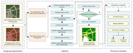
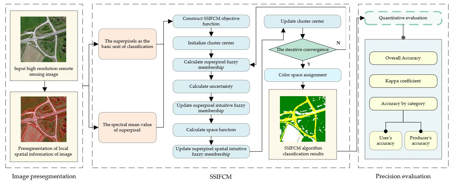
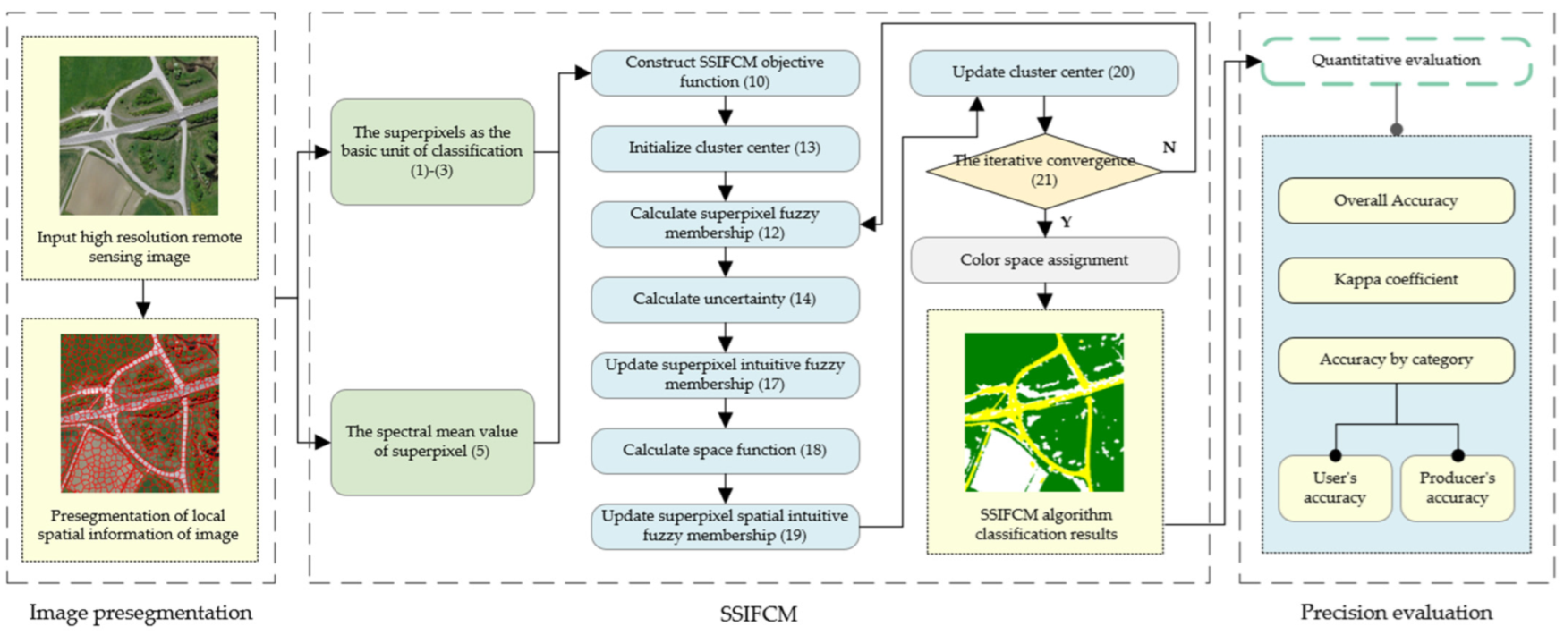
The overall technical flow of the proposed algorithm is shown in Figure 1.

3. Results

3.1. Experimental Data

Four scenes of HSRRS images from the aerial image dataset (AID) [30], published by Wuhan University and Huazhong University of Science and Technology in 2017, are used in this work. The dataset was created by collecting sample images from Google Earth imagery; the Google Earth images were post-processed using RGB renderings from the original optical aerial images. The dataset contains 10,000 images, including 30 scene types, such as airports, bare land, and forests; with approximately 220–420 images in each category, all the images are labelled by experts in remote sensing image interpretation. The images in this dataset are multi-sourced and come from different remote imaging sensors. Therefore, the images of AID have multi-resolutions, varying from 0.5 to 8 m, with a unified 600 × 600 pixels image size to cover a scene with various resolutions.

To verify the effectiveness and generalization ability of the proposed algorithm, four HSRRS images were selected from the AID (Figure 2). All the images contain three bands of red, green, and blue. The four HSRRS images mainly include buildings, roads, water, vegetation, and bare ground. The S1 image contains a large building with its own structure rules; the shape of vegetation and roads in the image is irregular, which can be used to verify the classification integrity of the classification algorithm in images with irregular regional shape. The S2 image includes roads, bare land, and vegetation. The proportion of the pixels in the image is unbalanced, which can be used to verify the stability of the classification algorithm for images with unbalanced samples. Images S3 and S4 contain rivers and lakes, and their boundaries with vegetation and bare ground are unclear, which can be used to verify the discriminability of the classification algorithm for staggered objects.

3.2. Accuracy Evaluation

In this paper, two groups of comparative experiments were designed. The first group is used to verify the influence of both pixels and objects as basic units on the spatial intuitionistic fuzzy clustering algorithm. The second group is used to verify the robustness of the proposed algorithm. Qualitative and quantitative methods were used to evaluate the accuracy of the classification results.

The quantitative evaluation of classification results is based on the confusion matrix method, and the rows of the matrix represent the predicted category. The leading indicators are as follows [31]: producer’s accuracy (PA), user’s accuracy (UA), overall accuracy (OA), and Kappa coefficient. The higher the above index value is, the better the classification effect.

The experimental platform is an Intel(R) Core (TM) six Core, 16 GB memory, Win10 operating system, and the software used includes MATLAB R2018b, Python 3.7, and PIE.

3.3. Experimental Results and Analysis

3.3.1. Experimental Comparison and Analysis of Pixel-Level and Object-Level Spatial Intuitive Fuzzy Clustering Algorithms

In this group of experiments, the pixel-level spatial intuitive FCM (PSIFCM) clustering algorithm [32] was used for comparison with the algorithm in this paper. Figure 3 shows the classification results of the pixel-level and object-level spatial intuitive fuzzy clustering algorithms. To facilitate visual analysis and comparison, red rectangular boxes are marked in the experimental results. Figure 3a,d,g,j are the reference images of the S1, S2, S3, and S4 images, respectively, which were obtained by manual visual interpretation.

As seen from the classification results, the PSIFCM in Figure 3b,c shows that the red rectangular labeled area produces a large amount of salt and pepper noise. The SSIFCM solves this problem effectively. In the S2 image, it is shown that PSIFCM misclassified vegetation and raw ground and produced ‘noise points’, resulting in a poor classification effect. In our algorithm, the noise was effectively removed, and the specific ability of ground objects was improved. In the S3 image, the water contour is irregular, the edge information is fuzzy, and both algorithms produce misclassification. However, in the red rectangular box in Figure 3h,i, the proposed algorithm improves the classification effect to a certain extent. The S4 image contains a large area of water, and ground objects have various categories but unknown boundaries, with significant differences within the categories. The denoising impact of the proposed algorithm is better than that of PSIFCM, and the visual effect of classification is the best.

Regarding classification accuracy, the building classification accuracy of PSIFCM in

Table 1. Evaluation of S1 image pixel-level and object-level spatial intuitive fuzzy clustering algorithms classification results.

S1	OA	Kappa	Vegetation		Load		Building
			PA	UA	PA	UA	PA	UA
PSIFCM	89.88%	84.71%	83.94%	87.49%	88.25%	85.86%	97.42%	96.98%
SSIFCM	92.89%	89.21%	90.71%	89.10%	89.89%	92.51%	98.72%	96.74%

is good, but the classification accuracy of vegetation and road is lower than 89.00%. In

Table 2. Evaluation of S2 image pixel-level and object-level spatial intuitive fuzzy clustering algorithms classification results.

S2	OA	Kappa	Vegetation		Load		Bare Land
			PA	UA	PA	UA	PA	UA
PSIFCM	82.27%	66.28%	98.91%	83.05%	96.23%	67.57%	42.75%	97.20%
SSIFCM	88.87%	77.50%	98.34%	89.89%	95.21%	78.83%	56.74%	96.39%

, PA values of PSIFCM vegetation and roads and UA values of raw ground are optimal, but other items are lower than the SSIFCM by 6–14%. In

Table 3. Evaluation of S3 image pixel-level and object-level spatial intuitive fuzzy clustering algorithms classification results.

S3	OA	Kappa	Vegetation		Bare Land		River
			PA	UA	PA	UA	PA	UA
PSIFCM	85.06%	77.63%	95.31%	70.14%	90.75%	96.01%	71.06%	98.29%
SSIFCM	89.78%	84.50%	95.61%	80.85%	93.91%	96.39%	79.25%	97.65%

, although the UA value of the PSIFCM algorithm is high, its PA value is only 71.06%, and our algorithm is superior to PSIFCM in other terms. In

Table 4. Evaluation of S4 image pixel-level and object-level spatial intuitive fuzzy clustering algorithms classification results.

S4	OA	Kappa	Vegetation		Lake
			PA	UA	PA	UA
PSIFCM	95.02%	90.00%	96.24%	93.19%	93.97%	96.68%
SSIFCM	96.44%	92.88%	95.30%	97.34%	97.53%	95.62%

, it is shown that the vegetation PA value and lake UA value of the proposed algorithm are slightly lower than those of the PSIFCM algorithm, and the other items are optimal. The overall accuracy and Kappa coefficients of the proposed algorithm are both higher than those of the PSIFCM algorithm, and 23 of the 30 evaluation indices are superior to those of PSIFCM.

Thus, the experiments verify that the SSIFCM is superior to PSIFCM in classification accuracy and visual effect.

3.3.2. Comparative Analysis with Main Unsupervised Classification Algorithms

In this group of experiments, results from the algorithm proposed in this paper were compared with fourteen unsupervised classification algorithms, including K-means [33], ISODATA [34], FCM [35], IFCM [36], fuzzy local information FCM (FLICM) clustering algorithm [37], the hidden Markov random field models-FCM (HMRF-FCM) clustering algorithm [38], the FCM clustering algorithm with spatial constraints (FCM_S) [39], the FCM clustering algorithm with spatial and intensity constraint and membership (FCM-SICM) [40], SFFCM [17], FRFCM [18], the superpixel-based FCM (SPFCM) clustering algorithm [41], the SLIC-back propagation neural network (SBPNN) [42], felzenszwalb-BPNN (FBPNN) [43], and the self-organization neural network (SOM) [44]. Among them, K-means, ISODATA, FCM, IFCM, FLICM, HMRF-FCM, FCM_S, FCM-SICM, and SOM are pixel-level classification algorithms, while SFFCM, FRFCM, SPFCM, SBPNN, FBPNN, and SSIFCM are object-level classification algorithms, SBPNN and FBPNN are deep-learning-based approaches.

(1)

S1 image experiment results

Figure 4 shows the experimental results for S1 image classification. As can be seen from the figure, vegetation and roads are easily misclassified. Six algorithms, including K-means, ISODATA, FLICM, HMRF-FCM, FBPNN, and SOM failed to distinguish between roads and vegetation. Four algorithms, including IFCM, FCM_S, FCM-SICM, and SFFCM misclassified some shadowed streets as vegetation. The IFCM, FCM_S, and FCM-SICM algorithms are greatly affected by salt and pepper noises. Three other algorithms, FCM, FRFCM, and SPFCM, have misclassification in the mixed region demarcated by the red rectangular box. Only SBPNN and the proposed algorithm solve the above problems and obtain the best classification effect. Compared with the classification results in

Table 5. Evaluation of S1 image classification results.

S1	OA	Kappa	Vegetation		Road		Building
			PA	UA	PA	UA	PA	UA
K-means	66.33%	46.81%	4.27%	0.70%	55.74%	93.01%	99.76%	92.25%
ISODATA	66.31%	46.78%	4.73%	0.79%	55.70%	92.69%	99.75%	92.48%
FCM	89.77%	84.50%	84.54%	85.32%	86.43%	87.93%	98.96%	96.02%
IFCM	80.45%	71.04%	62.47%	92.93%	87.99%	58.55%	98.68%	96.28%
FLICM	66.36%	46.89%	4.76%	0.81%	55.68%	92.27%	99.80%	93.16%
HMRF-FCM	54.22%	29.45%	12.38%	9.43%	49.56%	65.45%	98.45%	80.51%
FCM-S	80.34%	70.72%	63.19%	87.32%	83.70%	62.26%	98.98%	96.37%
FCM-SICM	84.29%	76.52%	69.09%	89.75%	87.93%	70.06%	98.66%	96.93%
SFFCM	70.42%	55.73%	49.15%	62.46%	66.37%	54.94%	99.66%	96.64%
FRFCM	91.04%	86.42%	86.82%	86.55%	87.89%	89.67%	98.96%	96.76%
SPFCM	90.53%	85.70%	82.89%	89.69%	89.47%	86.32%	99.47%	96.48%
SBPNN	91.95%	87.79%	95.12%	86.30%	90.34%	91.58%	91.42%	97.47%
FBPNN	68.12%	49.52%	4.24%	0.37%	55.86%	94.62%	99.90%	96.16%
SOM	66.29%	46.73%	3.57%	0.57%	55.73%	93.29%	99.76%	91.89%
SSIFCM	92.89%	89.21%	90.71%	89.10%	89.89%	92.51%	98.72%	96.74%

, we found that: the UA value of the IFCM algorithm is the best, but the PA value is only 62.47%, while the proposed algorithm reaches 90.71%. The UA value of the K-means algorithm is 0.50% higher than that of the proposed algorithm, but the PA value is 34.15% lower than that of the proposed algorithm. The SBPNN algorithm has three optimal indicators, which are equivalent to the proposed algorithm, but the latter obtains the best overall accuracy and Kappa coefficient. In general, the classification effect of the proposed algorithm is better than those of the comparison algorithms.

(2)

S2 image experiment results

As can be seen from Figure 5, vegetation near roads in the S2 image is characterized by strong spectral heterogeneity. Seven algorithms of IFCM, FCM-S, FCM-SICM, SFFCM, FRFCM, FBPNN, and SOM failed to distinguish the road from raw ground correctly. Six algorithms, including K-means, ISODATA, FCM, FLICM, HMRF-FCM, SPFCM, and SOM misclassified some vegetation as raw ground and produced many noise points. The SBPNN algorithm performed poorly in this set of experiments, and the classification was not robust. However, the proposed algorithm can distinguish all ground objects correctly and has a good suppression effect on the salt and pepper noises generated by the pixel-level classification algorithm. Quantitative analysis shows that the proposed algorithm is superior to the comparison algorithms in four aspects (

Table 6. Evaluation of S2 image classification results.

S2	OA	Kappa	Vegetation		Road		Bare Land
			PA	UA	PA	UA	PA	UA
K-means	80.30%	63.68%	98.95%	78.94%	95.92%	73.49%	39.93%	96.70%
ISODATA	74.89%	56.48%	99.19%	70.68%	94.98%	76.15%	33.91%	96.47%
FCM	80.42%	63.55%	98.75%	80.10%	95.98%	69.42%	40.17%	96.57%
IFCM	62.94%	36.92%	99.13%	66.59%	52.92%	91.07%	3.23%	6.03%
FLICM	83.13%	67.45%	98.89%	84.90%	97.73%	64.66%	43.87%	97.51%
HMRF-FCM	69.49%	47.00%	98.28%	70.43%	76.65%	56.33%	28.01%	81.52%
FCM-S	61.92%	37.21%	99.35%	62.58%	54.82%	77.56%	15.13%	37.83%
FCM-SICM	59.94%	34.42%	99.87%	61.15%	51.53%	94.38%	4.01%	8.22%
SFFCM	66.97%	36.32%	95.58%	62.25%	52.10%	92.45%	0.04%	0.07%
FRFCM	53.87%	28.71%	99.76%	52.49%	55.73%	93.03%	3.77%	10.33%
SPFCM	68.48%	46.95%	99.10%	65.78%	72.02%	85.88%	23.30%	60.65%
SBPNN	71.99%	52.04%	95.13%	63.54%	37.96%	93.67%	98.77%	90.29%
FBPNN	55.56%	27.62%	99.03%	59.97%	4.72%	8.43%	43.23%	92.86%
SOM	61.89%	35.71%	99.38%	65.57%	53.61%	87.88%	3.72%	7.60%
SSIFCM	88.87%	77.50%	98.34%	89.89%	95.21%	78.83%	56.74%	96.39%

). The overall accuracy, the Kappa coefficient and the UA value of vegetation improved by 5.65–35.00%, 10.01–49.88%, and 4.99–37.4%, respectively. The SBPNN algorithm achieved a bare ground PA value of 98.77% but had poor accuracy in other categories.

(3)

S3 image experiment results

Compared with the first two scenes, S3 is characterized by a fuzzy water boundary and an irregular shape (Figure 6). For the water and vegetation areas, all algorithms have a certain degree of misclassification and a large number of noise points generated, except the SFFCM algorithm. In summary, the FBPNN and the proposed algorithm have high integrity in distinguishing ground objects, and have a good smoothing effect on the salt and pepper noises. However, the FBPNN algorithm is not robust enough for classification in other images. As shown in

Table 7. Evaluation of S3 image classification.

S3	OA	Kappa	Vegetation		Bare Land		River
			PA	UA	PA	UA	PA	UA
K-means	83.92%	75.97%	94.75%	68.02%	86.92%	96.31%	71.56%	97.24%
ISODATA	84.60%	76.93%	94.67%	69.69%	86.92%	96.31%	73.03%	97.00%
FCM	84.40%	76.66%	94.58%	69.29%	87.47%	95.97%	72.30%	97.31%
IFCM	82.17%	73.52%	95.45%	63.39%	84.10%	97.04%	69.77%	97.65%
FLICM	85.63%	78.43%	95.01%	71.68%	88.57%	96.44%	73.89%	97.38%
HMRF-FCM	58.24%	38.83%	57.14%	33.45%	77.91%	59.17%	50.47%	99.16%
FCM-S	83.27%	74.91%	91.88%	68.69%	86.30%	93.54%	72.40%	96.66%
FCM-SICM	85.10%	77.69%	94.99%	70.38%	91.90%	95.58%	70.65%	98.53%
SFFCM	83.96%	75.79%	89.38%	72.89%	92.16%	88.07%	72.17%	98.20%
FRFCM	86.05%	79.07%	95.35%	72.34%	93.43%	95.88%	71.38%	98.47%
SPFCM	86.61%	79.88%	95.48%	73.56%	91.05%	96.78%	73.94%	97.56%
SBPNN	81.40%	72.35%	92.38%	63.79%	99.13%	92.15%	62.10%	99.40%
FBPNN	89.71%	84.37%	94.66%	81.61%	93.94%	95.12%	79.95%	97.50%
SOM	84.98%	77.48%	94.21%	70.86%	92.56%	95.55%	70.29%	97.28%
SSIFCM	89.78%	84.50%	95.61%	80.85%	93.91%	96.39%	79.25%	97.65%

, both the FBPNN and the proposed algorithm have three optimal indicators, but the overall classification accuracy and Kappa coefficient of the proposed algorithm are the best, with better performance in the other two indicators than the FBPNN algorithm. Although the UA values of bare ground and river of the proposed algorithm are slightly lower than those of the IFCM and HMRF-FCM algorithms, the PA values of bare ground and river are improved by 9.81% and 28.78%, respectively.

(4)

Experimental results of S4 image

Due to the uncertainty of the homogeneity area, some algorithms showed poor classification performance for the S4 image (Figure 7). K-means, ISODATA, and FCM are seriously affected by salt and pepper noises. Although the IFCM, FLICM, FCM-S, and FCM-SICM algorithms integrate other parameters on the basis of traditional algorithm, FBPNN and SOM algorithms use neural networks to gradually merge each region and cluster each pixel in the iteration, so salt and pepper noise still exists. HMRF-FCM produces considerable noise, as well as serious misclassification. By introducing superpixels in SFFCM, FRFCM, SPFCM, SBPNN, and the proposed algorithm, the salt and pepper noises can be effectively suppressed, but the SBPNN algorithm cannot suppress an excessive combination of small areas by the neural network in the iterative process, resulting in a loss of image detail. The overall accuracy and Kappa coefficient of the proposed algorithm are better than those of the comparison algorithm (

Table 8. Evaluation of S4 image classification results.

S4	OA	Kappa	Vegetation		Lake
			PA	UA	PA	UA
K-means	92.97%	85.86%	95.88%	89.09%	90.66%	96.51%
ISODATA	79.74%	58.64%	98.84%	58.20%	72.29%	99.38%
FCM	94.09%	88.14%	95.22%	92.24%	93.12%	95.78%
IFCM	94.02%	88.00%	95.46%	91.83%	92.80%	96.02%
FLICM	94.97%	89.92%	95.34%	94.05%	94.64%	95.81%
HMRF-FCM	79.19%	57.52%	97.74%	57.69%	71.92%	98.78%
FCM-S	94.24%	88.48%	92.77%	95.36%	95.66%	93.23%
FCM-SICM	95.48%	90.94%	95.14%	95.39%	95.79%	95.56%
SFFCM	95.23%	90.48%	91.94%	98.65%	98.68%	92.12%
FRFCM	96.23%	92.46%	93.81%	98.59%	98.66%	94.07%
SPFCM	95.98%	91.96%	94.11%	97.69%	97.82%	94.42%
SBPNN	92.02%	84.12%	85.67%	99.98%	99.98%	84.76%
FBPNN	94.24%	88.48%	91.68%	96.70%	96.83%	92.00%
SOM	91.91%	83.73%	94.35%	88.31%	89.94%	95.18%
SSIFCM	96.44%	92.88%	95.30%	97.34%	97.53%	95.62%

). The vegetation PA value and lake UA value of the ISODATA algorithm are the best, but the vegetation UA value and lake PA value are only 58.20% and 72.29%, respectively. The vegetation UA value and lake PA value of the SBPNN algorithm is higher than those of the proposed algorithm. Nevertheless, the vegetation PA value and lake UA value are much lower than those of the proposed algorithm by 9.63% and 10.86%, respectively. Overall, the proposed algorithm obtains the optimal classification accuracy. This collection of trials demonstrates the object-level classification algorithm’s ability in “suppressing” salt and pepper noise.

4. Discussion

The proposed algorithm achieved better performance in four HSRRS image experiments compared to the other fifteen algorithms, which demonstrates that SSIFCM is effective and feasible for HSRRS image classification with rich details. It can be seen from the experimental results that there are many factors affecting the accuracy of image classification, including but not limited to the complex backgrounds in images and uneven pixel ratios for each category.

The overall accuracy and Kappa coefficient in the S2 image experiment is lower than those of the S1 image, mainly because the S2 image has a wide variety of ground objects, different ground objects have spectral overlap, and the fuzzy boundary of contour information is not clear, so the classification is more difficult. The overall accuracy and Kappa coefficient of the S4 image are significantly improved, mainly because the content of the S4 image is singular compared with other images, meaning less ground objects need to be considered and the classification basis is easy to grasp.

Traditional pixel-level classification algorithms, such as K-means, ISODATA, and FCM, have relatively singular feature information, which means they cannot accurately express ground object information and are susceptible to salt and pepper noise, resulting in poor classification results. IFCM, FLICM, HMRF-FCM, FCM-S, and FCM-SICM reduced the disadvantages of the traditional algorithm and basically preserved the details of the ground features, but the performance remains to be improved. Superpixels introduced in the SFFCM, FRFCM, SPFCM, SBPNN, and FBPNN algorithms can suppress salt and pepper noise, but misclassification still exists.

SOM is a shallow neural network model, but SOM has no obvious advantages over other methods. SBPNN and FBPNN combine deep learning with autoencoder structures to classify the input images. SBPNN and FBPNN pre-segment the images by using the SLIC and Felzenszwalb algorithms, respectively, and then complete feature extraction of the input images using a full convolutional network. A convolution network can better perceive the difference in texture, not just rely on color to classify. However, SBPNN and FBPNN are not robust enough, the algorithms are greatly affected by parameters, and the results of the algorithms can vary with multiple random restarts. Besides, SBPNN and FBPNN cannot achieve instance segmentation in practical application, assigning the same label to pixels with similar semantics through iteration, is not fully applicable to HSRRS images with rich information. FBPNN is an improvement from SBPNN, which reduces the number of iterations, but leads to a decrease in accuracy. As can be seen in Figure 7l, the SBPNN algorithm does not suppress excessive merging of small regions by the neural network, which leads to a certain degree of detail loss.

Superpixel segmentation can reduce information redundancy and comprehensively utilize spectral and spatial information of images, but the classification uncertainty of some ground objects in HSRRS images still exists after superpixel segmentation. The introduction of intuitionistic fuzzy sets can better solve the classification uncertainty, and the control of spatial function on adjacent pixel weight can also effectively reduce the influence of noise on classification results, so as to improve the classification accuracy. In this paper, the algorithm can take into account the uncertainty of the characteristics of homogeneous regions, so that the uncertainty expression of pixel classes is enhanced, which optimizes the classification effect. The algorithm effectively solves the problem that some regions in the experiment are easily misclassified due to strong spectral heterogeneity and blurred boundaries, while effectively retaining boundary details, thus verifying the distinguishability of SSIFCM for boundary-crossing areas. Such as the vegetation and bare ground area in the S1 image red rectangle, it is also noted that the vegetation area marked by a red rectangle box in the S2 image is prone to misclassification.

The computational complexity of SSIFCM is well discussed and studied, and compared with SPFCM, SFFCM, and FRFCM, which has an overall better effect.

Table 9. The running time of SSIFCM for remote sensing images of different sizes and resolutions.

Spatial Resolution	Size of Image	Number of Clusters	Riming Time
0.1 m	200 × 200 pixels	4	1.6 s
0.1 m	400 × 400 pixels	4	5.7 s
0.1 m	600 × 600 pixels	4	9.1 s
0.1 m	800 × 800 pixels	4	14.3 s
0.1 m	1000 × 1000 pixels	4	28.4 s
0.1 m	1200 × 1200 pixels	4	40.4 s
0.1 m	1400 × 1400 pixels	4	79.5 s
0.1 m	200 × 200 pixels	4	1.8 s
0.2 m	200 × 200 pixels	4	2.4 s
0.3 m	200 × 200 pixels	4	1.2 s
0.4 m	200 × 200 pixels	4	2.0 s
0.5 m	200 × 200 pixels	4	2.6 s
0.6 m	200 × 200 pixels	4	2.1 s
0.7 m	200 × 200 pixels	4	1.4 s

shows a comparison of the computational complexity of the proposed algorithm when changing HSRRS size and spatial resolution. The experiments were conducted using raw UAV images of a local area in Anning City, Yunnan Province, with a spatial resolution of 0.1 m and an image size of 1706 × 1546 pixels, containing three bands of red, green, and blue. By clipping and resampling, seven images with the same spatial resolution and different image sizes, and seven images with the same image sizes and different spatial resolution were obtained, respectively, and used to explore the relationship between the computational complexity of the proposed algorithm and the spatial resolution and image size of remote sensing images. As can be seen in Table 9, image size is positively correlated with algorithm running time when the spatial resolution is the same. The larger the image, the more content it contains, and the more iterations the algorithm needs before reaching the threshold. When the image size is the same, the change in spatial resolution has no obvious correlation with the running time of the algorithm. The reason for this result may be that the proposed algorithm completes the pre-segmentation through superpixels before fuzzy clustering. We will conduct in-depth research on this issue in the future.

Table 10. Comparison of the running time of SSIFCM with SPFCM, SFFCM, and FRFCM.

S2	Riming Time	OA	Kappa
SPFCM	3.7 s	68.48%	46.95%
SFFCM	2.9 s	66.97%	36.32%
FRFCM	5.1 s	53.87%	28.71%
SSIFCM	9.4 s	88.87%	77.50%

compares the running time of the algorithm with SPFCM, SFFCM, and FRFCM using the S2 image. In terms of the running time, there is still a slight gap between the proposed algorithm and the comparison algorithm. The reason for this result may be that the proposed algorithm improved on the basis of BCFCM, which is insensitive to noise. Overall, the proposed algorithm is superior to SPFCM, SFFCM, and FRFCM in accuracy evaluation. Similarly, we will continue to optimize the algorithm for the problem of running time in the future.

5. Conclusions

In this paper, an unsupervised classification algorithm (SSIFCM) for HSRRS images was proposed to cope with the problems pixel-level HSRRS image unsupervised classification, such as the ease of producing salt and pepper noises, serious misclassification, and classification uncertainty. By introducing IFS and spatial functions, the membership function was modified to a superpixel spatial intuitionistic fuzzy membership matrix that considered the classification of uncertainty, membership degree, and non-membership degree simultaneously. The limitation of single membership clustering is balanced in this work to solve the problems of uncertain classification and the similar feature intensity of adjacent pixels that are easily classified into the same category, which ensures the classification accuracy.

Four HSRRS images in the AID were selected for verification. The overall accuracy and Kappa coefficients of the proposed algorithm were better than those of the comparison algorithm. The overall accuracy improved by 0.21~38.67% and the Kappa coefficient was improved by 0.42~59.76%. Compared with the sound SFFCM and FRFCM, the proposed algorithm outperformed the FRFCM in 22 and the SFFCM in 23 out of 30 indices in 4 groups of experiments.

Further research will be conducted considering edge features and graph cutting to improve the classification performance and adaptively determine the initial parameters of superpixels and the number of classification categories.

References

1. Cheng, G.; Xie, X.X.; Han, J.; Guo, L.; Xia, G.S. Remote Sensing Image Scene Classification Meets Deep Learning: Challenges, Methods, Benchmarks, and Opportunities. IEEE J. Sel. Top. Appl. Earth Obs. Remote Sens. 2020, 13, 3735–3756. [Google Scholar] [CrossRef]
2. Li, D.R.; Ding, L.; Shao, Z.F. Application-Oriented Real-Time Remote Sensing Service Technology. Natl. Remote Sens. Bull. 2021, 25, 15–24. [Google Scholar]
3. Chen, T.; Zhao, Y.; Guo, Y.R. Sparsity-Regularized Feature Selection for Multi-class Remote Sensing Image Classification. Neural Comput. Appl. 2019, 32, 6513–6521. [Google Scholar] [CrossRef]
4. Zadeh, L.A. Fuzzy Sets as a Basis for a Theory of Possibility. Fuzzy Sets Syst. 1999, 100, 9–34. [Google Scholar] [CrossRef]
5. Zhang, H.; Wang, Q.M.; Shi, W.Z.; Hao, M. A Novel Adaptive Fuzzy Local Information C-Means Clustering Algorithm for Remotely Sensed Imagery Classification. IEEE Trans. Geosci. Remote Sens. 2017, 55, 5057–5068. [Google Scholar] [CrossRef]
6. Wang, C.; Pedrycz, W.; Li, Z.W.; Zhou, M.C. Residual-Driven Fuzzy C-Means Clustering for Image Segmentation. IEEE CAA J. Autom. Sin. 2021, 8, 876–889. [Google Scholar] [CrossRef]
7. Cohen, A.; Dahmen, W.; DeVore, R. Adaptive wavelet methods II—Beyond the elliptic case. Found. Comput. Math. 2002, 2, 203–245. [Google Scholar] [CrossRef]
8. Cherfa, I.; Mokraoui, A.; Mekhmoukh, A. Adaptively Regularized Kernel-Based Fuzzy C-Means Clustering Algorithm Using Particle Swarm Optimization for Medical Image Segmentation. In Proceedings of the 24th IEEE Conference on Signal Processing: Algorithms, Architectures, Arrangements, and Applications (IEEE SPA), Electr Network, 23–25 September 2020; pp. 24–29. [Google Scholar]
9. Miao, J.Q.; Zhou, X.B.; Huang, T.Z. Local Segmentation of Images Using an Improved Fuzzy C-Means Clustering Algorithm Based on Self-adaptive Dictionary Learning. Appl. Soft Comput. J. 2020, 91, 106200. [Google Scholar] [CrossRef]
10. Askari, S. Fuzzy C-Means Clustering Algorithm for Data with Unequal Cluster Sizes and Contaminated with Noise and Outliers: Review and Development. Expert Sys. Appl. 2020, 165, 113856. [Google Scholar] [CrossRef]
11. Mai, D.S.; Long, T.N.; Le, H.T.; Hagras, H. A Hybrid Interval Type-2 Semi-Supervised Possibilistic Fuzzy C-Means Clustering and Particle Swarm Optimization for Satellite Image Analysis. Inf. Sci. 2021, 548, 398–422. [Google Scholar] [CrossRef]
12. Xu, Z.; Wu, J. Intuitionistic Fuzzy C-Means Clustering Algorithms. J. Syst. Eng. Electron. 2010, 4, 580–590. [Google Scholar] [CrossRef]
13. Huang, L.; Peng, Q.Z.; Yu, X.Q. Change Detection in Multitemporal High Spatial Resolution Remote-Sensing Images Based on Saliency Detection and Spatial Intuitionistic Fuzzy C-Means Clustering. J. Spectrosc. 2020, 2020, 2725186. [Google Scholar] [CrossRef]
14. Jin, D.R.; Bai, X.Z. Distribution Information Based Intuitionistic Fuzzy Clustering for Infrared Ship Segmentation. IEEE Trans. Fuzzy Syst. 2020, 28, 1557–1571. [Google Scholar] [CrossRef]
15. Ren, X.F.; Malik, J. Learning a Classification Model for Segmentation. In Proceedings of the IEEE International Conference on Computer Vision, Nice, France, 13–16 October 2003; pp. 10–17. [Google Scholar]
16. Wang, M.R.; Liu, X.B.; Gao, Y.X.; Ma, X.; Soomro, N.Q. Superpixel Segmentation: A Benchmark. Signal Process Image Commun. 2017, 56, 28–39. [Google Scholar] [CrossRef]
17. Lei, T.; Jia, X.H.; Zhang, Y.N.; Liu, S.G.; Meng, H.Y.; Nandi, A.K. Superpixel-Based Fast Fuzzy C-Means Clustering for Color Image Segmentation. IEEE Trans. Fuzzy Syst. 2018, 27, 1753–1766. [Google Scholar] [CrossRef] [Green Version]
18. Lei, T.; Jia, X.H.; Zhang, Y.N.; He, L.F.; Meng, H.Y.; Nandi, A.K. Significantly Fast and Robust Fuzzy C-Means Clustering Algorithm Based on Morphological Reconstruction and Membership Filtering. IEEE Trans. Fuzzy Syst. 2018, 26, 3027–3041. [Google Scholar] [CrossRef] [Green Version]
19. Singh, N.K.; Singh, N.J.; Kumar, W.K. Image Classification Using SLIC Superpixel and FAAGKFCM Image Segmentation. IET Image Proc. 2020, 14, 487–494. [Google Scholar] [CrossRef]
20. Ji, S.F.; Zhu, H.Q.; Wang, P.Y.; Ling, X.F. Image Clustering Algorithm Using Superpixel Segmentation and Non-Symmetric Gaussian–Cauchy Mixture Model. IET Image Proc. 2020, 14, 4132–4143. [Google Scholar] [CrossRef]
21. Huang, L.; Yao, B.X.; Chen, P.D.; Yang, X.; Fu, B.H. Superpixel Segmentation Method of High-Resolution Remote Sensing Image Based on Fuzzy Clustering. Cehui Xuebao 2020, 49, 589–597. [Google Scholar]
22. Huang, L.; Yao, B.X.; Chen, P.D.; Ren, A.P.; Xia, Y. Superpixel Segmentation Method of High Resolution Remote Sensing Images Based on Hierarchical Clustering. Hongwai Yu Haomibo Xuebao 2020, 39, 263–272. [Google Scholar]
23. Achanta, R.; Shaji, A.; Smith, K.; Lucchi, A.; Fua, P.; Susstrunk, S. SLIC Superpixels Compared to State-of-the-Art Superpixel Methods. IEEE Trans. Pattern Anal. Mach. Intell. 2012, 34, 2274–2282. [Google Scholar] [CrossRef] [Green Version]
24. Hu, F.; Xia, G.S.; Hu, J.W.; Zhang, L.P. Transferring Deep Convolutional Neural Networks for the Scene Classification of High-Resolution Remote Sensing Imagery. Remote Sens. 2015, 7, 14680–14707. [Google Scholar] [CrossRef] [Green Version]
25. Ahmed, M.N.; Yamany, S.M.; Mohamed, N.; Farag, A.A.; Moriarty, T. A Modified Fuzzy C-Means Algorithm for Bias Field Estimation and Segmentation of MRI Data. IEEE Trans. Med. Imaging 2002, 21, 193–199. [Google Scholar] [CrossRef]
26. Atanassov, K.T. Intuitionistic Fuzzy Sets. Fuzzy Sets Syst. 1986, 20, 87–96. [Google Scholar] [CrossRef]
27. Xu, Z.S. Intuitionistic Fuzzy Aggregation Operators. IEEE Trans. Fuzzy Syst. 2007, 15, 1179–1187. [Google Scholar]
28. Yager, R.R. On the Measures of Fuzziness and Negation Part II Lattices. Inf. Control 1980, 44, 236–260. [Google Scholar] [CrossRef] [Green Version]
29. Sugeno, M. Fuzzy Measures and Fuzzy Integrals—A Survey. In Readings in Fuzzy Sets for Intelligent Systems; Elsevier: Amsterdam, The Netherlands, 1993; pp. 251–257. [Google Scholar]
30. Xia, G.S.; Hu, J.W.; Hu, F.; Shi, B.G.; Bai, X.; Zhong, Y.F.; Zhang, L.P.; Lu, X.Q. AID: A Benchmark Data Set for Performance Evaluation of Aerial Scene Classification. IEEE Trans. Geosci. Remote Sens. 2017, 55, 3965–3981. [Google Scholar] [CrossRef] [Green Version]
31. Silvan-Cardenas, J.L.; Wang, L. Sub-Pixel Confusion-Uncertainty Matrix for Assessing Soft Classifications. Remote Sens. Environ. 2008, 112, 1081–1095. [Google Scholar] [CrossRef]
32. Tripathy, B.K.; Basan, A.; Govel, S. Image segmentation using spatial intuitionistic fuzzy C means clustering. In Proceedings of the 5th IEEE International Conference on Computational Intelligence and Computing Research (IEEE ICCIC), Park Coll Engn & Tekhnol, Coimbatore, India, 18–20 December 2014; pp. 878–882. [Google Scholar]
33. Kanungo, T.; Mount, D.M.; Netanyahu, N.S.; Piatko, C.D.; Silverman, R.; Wu, A.Y. An Efficient K-Means Clustering Algorithm: Analysis and Implementation. IEEE Trans. Pattern Anal. Mach. Intell. 2002, 24, 881–892. [Google Scholar] [CrossRef]
34. Irvin, B.J.; Ventura, S.J.; Slater, B.K. Fuzzy and Isodata Classification of Landform Elements from Digital Terrain Data in Pleasant Valley, Wisconsin. Geoderma 1997, 77, 137–154. [Google Scholar] [CrossRef]
35. Dembele, D.; Kastner, P. Fuzzy C-means method for clustering microarray data. Bioinformatics 2003, 19, 973–980. [Google Scholar] [CrossRef] [Green Version]
36. Kim, T.H.; Park, D.C.; Woo, D.M.; Han, S.S.; Lee, Y. MRI Image Segmentation Using Intuitive Fuzzy C-Means Algorithm. In Proceedings of the 2011 International Conference on Computer, Electrical, and Systems Sciences, and Engineering (CESSE 2011), Wuhan, China, 10–11 April 2011; pp. 306–309. [Google Scholar]
37. Krinidis, S.; Chatzis, V. A Robust Fuzzy Local Information C-Means Clustering Algorithm. IEEE Trans. Image Process. 2010, 19, 1328–1337. [Google Scholar] [CrossRef] [PubMed]
38. Chatzis, S.P.; Varvarigou, T.A. A Fuzzy Clustering Approach toward Hidden Markov Random Field Models for Enhanced Spatially Constrained Image Segmentation. IEEE Trans. Fuzzy Syst. 2008, 16, 1351–1361. [Google Scholar] [CrossRef]
39. Chen, S.C.; Zhang, D.Q. Robust Image Segmentation Using FCM with Spatial Constraints Based on New Kernel-Induced Distance Measure. IEEE Trans. Syst. Man Cybern. Part B Cybern. 2004, 34, 1907–1916. [Google Scholar] [CrossRef] [Green Version]
40. Wang, Q.S.; Wang, X.P.; Fang, C.; Yang, W.T. Robust Fuzzy C-means Clustering Algorithm with Adaptive Spatial & Intensity Constraint and Membership Linking for Noise Image Segmentation. Appl. Soft Comput. J. 2020, 92, 106318. [Google Scholar]
41. Wu, C.; Zheng, J.B.; Feng, Z.N.; Zhang, H.W.; Zhang, L.; Cao, J.W.; Yan, H. Fuzzy SLIC: Fuzzy Simple Linear Iterative Clustering. IEEE Trans. Circuits Syst. Video Technol. 2021, 31, 2114–2124. [Google Scholar] [CrossRef]
42. Kanezaki, A. Unsupervised Image Segmentation by Backpropagation. In Proceedings of the IEEE International Conference on Acoustics, Speech and Signal Processing (ICASSP), Calgary, Canada, 15–20 April 2018; pp. 1543–1547. [Google Scholar]
43. Unsupervised-Segmentation. Available online: https://github.com/Yonv1943/Unsupervised-Segmentation/tree/master (accessed on 19 June 2019).
44. Guo, Y.P. Unsupervised Classification of High Spectral Resolution Images Using the Kohonen Self-Organization Neural Network. Hongwai Yu Haomibo Xuebao 1994, 13, 409–417. [Google Scholar]
Figure 1. Flow chart of the proposed SSIFCM HSRRS image unsupervised classification algorithm.
Remotesensing 14 03490 g001
Figure 2. Remote sensing images. (a) S1 image, (b) S2 image, (c) S3 image, and (d) S4 image.
Remotesensing 14 03490 g002
Figure 3. Experimental results. The red rectangle boxes are selected as the comparison areas. (a) S1 reference images, (b) S1 sIFCM, (c) S1 SSIFCM, (d) S2 reference images, (e) S2 sIFCM, (f) S2 SSIFCM, (g) S3 reference images, (h) S3 sIFCM, (i) S3 SSIFCM, (j) S4 reference images, (k) S4 sIFCM, and (l) S4 SSIFCM.
Remotesensing 14 03490 g003
Figure 4. Experiment results of S1 images. The red rectangle boxes are selected as the comparison areas. (a) S1 K-means, (b) S1 ISODATA, (c) S1 FCM, (d) S1 IFCM, (e) S1 FLICM, (f) S1 HMRF-FCM, (g) S1 FCM_S, (h) S1 FCM-SICM, (i) S1 SFFCM, (j) S1 FRFCM, (k) S1 SPFCM, (l) S1 SBPNN, (m) S1 FBPNN, (n) S1 SOM, and (o) S1 SSIFCM.
Remotesensing 14 03490 g004
Figure 5. Experiment results of S2 images. The red rectangle boxes are selected as the comparison areas. (a) S2 K-means, (b) S2 ISODATA, (c) S2 FCM, (d) S2 IFCM, (e) S2 FLICM, (f) S2 HMRF-FCM, (g) S2 FCM_S, (h) S2 FCM-SICM, (i) S2 SFFCM, (j) S2 FRFCM, (k) S2 SPFCM, (l) S2 SBPNN, (m) S2 FBPNN, (n) S2 SOM, and (o) S2 SSIFCM.
Remotesensing 14 03490 g005aRemotesensing 14 03490 g005b
Figure 6. Experiment results of S3 images. The red rectangle boxes are selected as the comparison areas. (a) S3 K-means, (b) S3 ISODATA, (c) S3 FCM, (d) S3 IFCM, (e) S3 FLICM, (f) S3 HMRF-FCM, (g) S3 FCM_S, (h) S3 FCM-SICM, (i) S3 SFFCM, (j) S3 FRFCM, (k) S3 SPFCM, (l) S3 SBPNN, (m) S3 FBPNN, (n) S3 SOM, and (o) S3 SSIFCM.
Remotesensing 14 03490 g006aRemotesensing 14 03490 g006b
Figure 7. Experiment results of S4 images. The red rectangle boxes are selected as the comparison areas. (a) S4 K-means, (b) S4 ISODATA, (c) S4 FCM, (d) S4 IFCM, (e) S4 FLICM, (f) S4 HMRF-FCM, (g) S4 FCM_S, (h) S4 FCM-SICM, (i) S4 SFFCM, (j) S4 FRFCM, (k) S4 SPFCM, (l) S4 SBPNN, (m) S4 FBPNN, (n) S4 SOM, and (o) S4 SSIFCM.
Remotesensing 14 03490 g007