Article

The West Kunlun Glacier Anomaly and Its Response to Climate Forcing during 2002–2020

1
Jiangsu Provincial Key Laboratory of Geographic Information Science and Technology, Key Laboratory for Land Satellite Remote Sensing Applications of Ministry of Natural Resources, School of Geography and Ocean Science, Nanjing University, Nanjing 210023, China
2
Jiangsu Center for Collaborative Innovation in Novel Software Technology and Industrialization, Nanjing 210023, China
3
Collaborative Innovation Center of South China Sea Studies, Nanjing 210023, China
4
Institute of Geography, Friedrich-Alexander-Universität Erlangen-Nürnberg, 91054 Erlangen, Germany
*
Author to whom correspondence should be addressed.
Remote Sens. 2022, 14(14), 3465; https://doi.org/10.3390/rs14143465
Submission received: 23 April 2022 / Revised: 28 June 2022 / Accepted: 15 July 2022 / Published: 19 July 2022
(This article belongs to the Topic Cryosphere: Changes, Impacts and Adaptation)

Abstract

:
Research into glacial mass change in West Kunlun (WK) has been sufficient, but most of the existing studies were based on geodetic methods, which are not suitable for specific health state analyses of each glacier. In this paper, we utilize Advanced Spaceborne Thermal Emission and Reflection Radiometer (ASTER) imagery, applying the continuity equation to obtain altitudinal specific mass balance (SMB) for 615 glaciers (>2 km 2 ) during 2002–2011, 2011–2020, and 2002–2020 to research glacial health and its response to climatic forcing. The results show dissimilar glacier SMB patterns between 2002–2011 (0.10 ± 0.14 m w.e. a 1 ), 2011–2020 (–0.12 ± 0.14 m w.e. a 1 ) and 2002–2020 (−0.01 ± 0.07 m w.e. a 1 ). Additionally, the glacier equilibrium line altitude (ELA) in WK was 5788 m, 5744 m, and 5786 m, respectively, and the corresponding accumulation area ratios (AARs) were 0.59, 0.62, and 0.58, during 2002–2011, 2011–2020, and 2002–2020, respectively. Regarding glacier response, compared with the ordinary-least-square (OLS) model, the artificial neural network (ANN) model revealed a respectively less and more sensitive glacier SMB response to extreme negative and positive summer skin temperatures. In addition, the ANN model indicated that the glacier ELA was less sensitive when the integrated water vapor transport (IVT) change exceeded 0.7 kg m 1 s 1 . Moreover, compared with IVT (−121.57 m/ kg   m 1 s 1 ), glacier ELA shifts were chiefly dominated by summer skin temperature (+154.66 m/ ) in the last two decades. From 2002–2011 and 2011–2020, glacier SMB was more susceptible to summer skin temperature (−0.38 m w.e./ and −0.16 m w.e./ , respectively), while during 2002–2020, it was more influenced by IVT (0.45 m w.e./ kg   m 1 s 1 ). In contrast with eastern WK, glaciers in western WK were healthier, although mitigation measures are still needed to safeguard glacier health and prevent possible natural hazards in this region. Finally, we believe that the inconsistent change between glacier SMB and ELAs from 2002–2020 was connected with ice rheology and that the combined effects of skin temperature and IVT can explain the WK glacier anomaly.

1. Introduction

In the past two decades, glaciers worldwide have experienced accelerated ice mass loss due to global warming [1,2], which will result in more than one billion people facing water shortages and food insecurity in the upcoming three decades [3,4]. High Mountain Asia (HMA), regarded as “The Third Pole” [5], contains approximately 7.0 ± 1.8 ×   10 3   km 3 ice [6] and includes 95,536 glaciers with a total area of approximately 97,605 ± 7935 km 2 , based on the Randolph Glacier Inventory version 6.0 (RGI v6.0) [7,8]. Accordingly, it is crucial for glaciologists to research glacier change in HMA [9]. Previous studies have concluded that in Karakoram, West Kunlun (WK), Eastern Hindu Kush, and Eastern Pamir, glacier mass balance has been neutral or slightly positive in the last two decades [10,11,12,13,14,15]. Although numerous studies of glacier elevation or mass change in eastern WK have been undertaken [16,17,18], research into comprehensively and spatiotemporal glacier specific mass balance (SMB) change in WK is still lacking.
Additionally, via laser altimeters, optical stereo images, or interferometric synthetic aperture radar (InSAR) previous studies have estimated that glaciers in WK have been in a state of mass gain for the last two decades [15,19,20,21]. However, these glacier mass balance results were estimated from surface elevation change datasets and typically used a fixed area-averaged glacier surface density [22]. In contrast, glacier SMB should be determined by solving the continuity equation, considering depth-integrated ice flow, and applying varied ice density on the glacier surface, which is more robust and accurate, and more suitable for evaluating glacier health [23].
Moreover, glacier equilibrium line altitude (ELA) has been estimated by many glaciologists in high-mountain environments [24,25,26]. ELA is defined as the altitude line where over a period of one year, the accumulation of snow is exactly balanced by ablation [27,28]. There have been many studies about how to retrieve ELA based on the relationship between glacier mass balance and altitude profile [29,30,31]. However, these methods require prior knowledge of the glacier mass balance altitude curve, and in most cases, computation of ELA acquisition is time-consuming; thus, application of this ELA-retrieving approach has been limited. Other studies have acquired ELA by measuring the end-of-summer snow line altitude via optical imagery [32,33] or solely retrieving ELA from >7% or >10 km 2 of debris-covered areas for each glacier [34]. The latter technique assumes that previously existing debris cover (>1 year) is located within the ablation zone, and newly exposed debris on the glacier surface (<1 year), which remains more than one year after its exposure and survives in the accumulation zone. However, due to cloud cover effects on optical images and limited debris-covered glaciers worldwide, this method has restricted applications. In the current study, we acquired the ELA for each glacier by applying the Dice coefficient approach based on glacier SMB outcomes across WK during 2002–2020, which is less restricted and more robust than previous methods [23].
Previous studies have concluded that glacier mass balance is linearly sensitive to climatic factors (i.e., temperature, precipitation, radiation, humidity, and wind speed) [35,36,37,38,39,40,41], and bare-ice albedo [42]. Conversely, Bolibar et al. [43] confirmed that glacier mass balance response to meteorological factors is nonlinear. Furthermore, some studies have also concluded that glacier ELA shifts are correlated with climatic factors [27,44,45]. However, we discovered that previous studies primarily estimated glacier mass balance and ELAs through energy and mass balance models, based on meteorological reanalysis datasets or gauge station measurements. Owing to the scarcity of climatological stations in high-mountain regions, and the inaccuracy of climatic reanalysis datasets, the extent of glacier sensitivity to climatic factors remains uncertain. Compared with the energy and mass balance model, estimating glacier mass balance via continuity is more feasible and reliable because it relies on proven techniques (geodetic method, glacier velocity generation, and ice thickness estimation). Hence, in this study, we applied a continuity equation to obtain glacier SMB in WK, and to investigate nonlinear glacier SMB and ELA sensitivity to climatic elements in this area during 2002–2020, via the artificial neural network (ANN) technique [46].
In this study, we calculated spatially distributed SMB via the continuity equation during 2002–2020 and its two subperiods (2002–2011, 2011–2020), for each glacier across the whole WK and its two subregions, Western WK and Eastern WK. Glacier dynamics dataset were sourced from the ITS_LIVE project [47], and glacier thickness data were supplied by Farinotti et al. [6]. Additionally, we estimated ELAs and accumulation area ratios (AARs) for each glacier to research glacier health during 2002–2020. Finally, we utilized the ERA5.1 reanalysis dataset [48] to yield the mean annual skin temperature and integrated water vapor transport (IVT) trends during 2002–2020, and estimate the nonlinear response to these of glacier SMB and ELA in WK in the last two decades. Overall, the contribution of this work can be summarized into three points: (A) obtaining via continuity equation the multi-temporal glacier SMB in WK and its two subregions during 2002–2011, 2011–2020, and 2002–2020; (B) estimating via Dice coefficient the multi-temporal glacier ELA and AAR variation in WK in the past two decades; (C) researching nonlinear glacier SMB and ELA response to climate change in WK during 2002–2020.

2. Materials and Methods
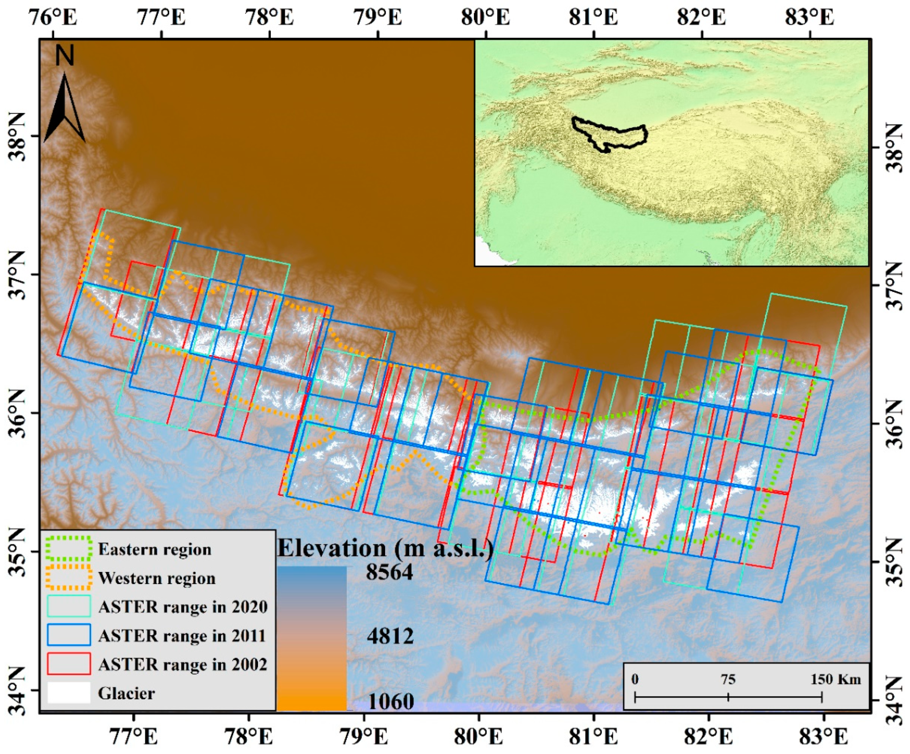
2.1. Study Area

WK ( 35 37 N, 76 83 E) is widely covered by glaciers (see Figure 1). We divided WK into two subregions, western WK and eastern WK. Based on RGI v6.0, WK includes 4819 glaciers, and the total area of glaciers (>0.01 km 2 ) is 7855 km 2 , making it one of the most extensively glaciated areas in China. In western WK and eastern WK, there are 2958 glaciers (2899 km 2 ) and 1861 glaciers (4956 km 2 ), respectively. These glaciers are characterized as cirque, valley, and ice-cap types. Herreid and Pellicciotti [34] found that the area of debris-covered glaciers in WK was 245 km 2 . The Guliya Ice Cap is the largest ice cap in mainland Asia (~370 km 2 ) [49], and the Duofeng glacier, the largest mountain glacier in the WK, has an area of ~240 km 2 . The main ridge of WK separates the steep northern slope, descending to the Tarim Basin, and the southern slope, which has a lower gradient towards the Tibetan Plateau [50,51]. The local climate is frigid and dry and is primarily controlled by midlatitude westerlies. The annual precipitation and mean temperature near the ELA (~5930 m a.s.l.) are approximately 300 mm (mainly concentrated in May–September) and −13.9 , respectively [52]. Summer accumulation is dominant for glaciers in WK [53].

2.2. Data

This study calculated glacier SMB by the continuity equation, leveraging Advanced Spaceborne Thermal Emission and Reflection Radiometer (ASTER) DEMs, ITS_LIVE ice velocity, and ice thickness during 2002–2011, 2011–2020, and 2002–2020 (Supplementary Information Tables). In addition, we used the ERA 5.1 reanalysis dataset to obtain the annual mean skin temperature and IVT trends in WK from 2002–2020 (see Table 1).

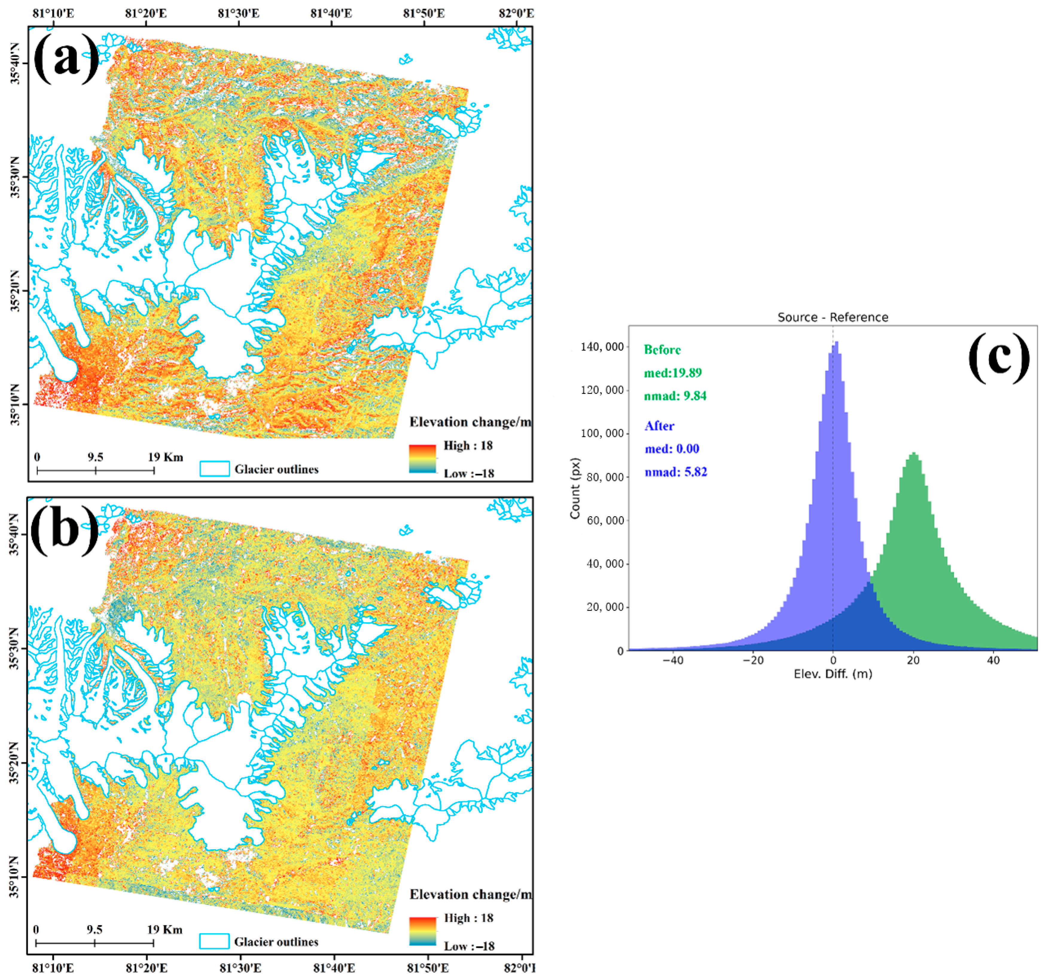
2.3. Glacial Elevation Change Generation

To provide full coverage of glaciers in WK in 2002, we used ASTER DEMs from 2001, 2003, 2004, and 2005 to compensate for the dearth of ASTER image coverage in 2002. This situation also occurred in 2011 and 2020. We chose 2002, 2011, and 2020 as representatives because the greatest quantities of ASTER imagery were available for these three time points. We calculated the elevation change for each glacier within its own specific time offset (Supplementary Information Discussion). In addition, we chose predominantly winter and spring ASTER images because they could minimize seasonal offset when acquiring glacier elevation change (hereafter referred to as “seasonal bias”) [54]. To account for the seasonal bias, we used a winter accumulation rate of +0.15 m per month [55,56].
We used MicMac ASTER software to obtain ASTER DEMs. We chose this software because it could provide higher-accuracy DEMs with sensor motion (“jitter”) correction, compared with silcAst software [57]. Next, we applied the methods proposed by Nuth and Kääb [58] to coregister DEMs for 2002, 2011, and 2020 (excluding glacier area using RGI v6.0), to obtain glacier elevation change results for the three different periods. Here, we used ASTER DEMs from 2020 as a primary map to coregister ASTER DEMs from 2002 and 2011. In addition, during the coregistration procedure, we applied fifth-order polynomial correction for curvature bias, which has been described and applied previously [11,59]. One example of the coregistration results can be seen in Figure 2. Here, we used Median and Normalized Median Absolute Deviation (NMAD) as statistical tools to evaluate the effects of DEM coregistration [60].
Furthermore, after we obtained glacier elevation change in WK, we used ASTER DEMs for the three different periods to acquire the corresponding slope map, and then excluded from the slope map glacier elevation change pixels >   45 ° to eliminate erroneous pixels in the glacier elevation change maps [61].

2.4. SMB Obtainment

2.4.1. Continuity Equation

In this study, we used the continuity Equation (1) to calculate SMB for each glacier in WK [62,63,64]:
H t = b q
where H t is the annual rate of elevation change on the glacier surface and b is the annual SMB, including the surface, internal, and basal mass balance combined; here, however, we refer to b as the surface mass change, assuming that frontal ablation englacial and subglacial components are negligible [65,66]. q is the annual ice flux divergence. All these equation elements are in the unit of meters of ice equivalent per year (m, i.e., a 1 ). To transfer each unit into meters of water equivalent per year (m w.e. a 1 ), we can modify and reorganize Equation (1) into Equation (2):
b w = H t ρ H ρ H 2 O + q ρ q ρ H 2 O
where b w refers to SMB in meters of water equivalent per year [23]. ρ H and ρ q are ice densities on the glacier surface, ρ H 2 O is the water density (999.972 kg m 3 ).

2.4.2. Ice Flux and Flux Divergence

To acquire glacier SMB, it was necessary to obtain ice flux divergence. We calculated the ice flux vector at each pixel according to Equation (3), with the ITS_LIVE multiyear mean ice velocity dataset for three periods (2002–2011, 2011–2020, and 2002–2020) and the modelled glacier thickness dataset. Surging glaciers were not excluded, because Yasuda and Furuya [51] concluded that there were only three surging glaciers in the West Kunlun Shan from 2000 to 2014, while Dehecq et al. [47] reported that there were only seven glaciers in a surging state.
q = H γ V s
where q represents the ice flux vector, H is the ice thickness in meters, γ V s is the column-averaged glacier velocity, and the constant γ represents the relative importance of basal motion and vertical ice shear deformation. To determine γ for each glacier, we applied a Monte Carlo analysis to estimate the depth-integrated velocity per pixel [23].
The ice flux divergence represents the vertical component of glacier surface velocities, resulting in submergence in divergent flow zones and emergence in convergent flow zones. Based on this, we calculated ice flux divergence q using Equation (4) [23]:
q = q x x + q y y
where q x x and q y y represent ice flux divergence values in the x and y directions, respectively.

2.4.3. Density Correction

In this study, we used transformed Equation (2) to obtain SMB as the unit of meters of water equivalent per year (m w.e. a 1 ). Thus, it was necessary to consider glacier surface density variations. We did not consider temporal mean ice density variation, because this led to an uncertainty of only 2% [67]. Nevertheless, we had to consider the ice density variation between the accumulation and ablation zones of each glacier, and the dissimilarity of snow and ice densities. In general, snow and firn usually have a lower density than clean ice [68].
We took three steps to correct glacier density. First, we assumed that clean ice was the dominant type spreading over the glacier surface; thus, we gave each glacier an ice density of 900 kg   m 3 . After that, we combined the elevation change signal and flux divergence to classify the accumulation and ablation zones for each glacier. If elevation change and flux divergence were both positive, we regarded this area as an accumulation zone and assigned a density of 600 kg   m 3 . If they both represented negative values, we assumed this corresponded to the glacier ablation zone, and a density of 900 kg   m 3 was assigned. Finally, for the rest of the glacier area, we assumed a density of 850 kg   m 3 . We assumed that glacier density uncertainty was 60 kg   m 3 [23].

2.5. Uncertainty Estimations

2.5.1. Uncertainty of Glacial Elevation Change

We suggest that elevation change uncertainty involves three factors: residual bias related to DEM coregistration, glacier area change, and voids in the DEM difference map. Here, we calculated the glacier elevation change uncertainty by Equation (5):
E Δ h = E c o r e g 2 + E a r e a 2 + E v o i d s 2
where E Δ h represents the glacier elevation change uncertainty and E c o r e g is the uncertainty associated with the residual error in the stable area of the DEM difference maps after DEM coregistration. E a r e a represents the uncertainty caused by glacier area changes in the last 20 years. E v o i d s refers to the void-filling method [69], leading to offsetting of glacier elevation change.
We assert that in the same slope range, the elevation changes in the stable area and glaciated area have the same elevation change offset patterns, which has been described previously [70,71]. To acquire stable regions, we excluded lakes according to the HydroLAKES v1.0 dataset [72]. We also tried to remove glacial lake impacts [73] from the DEM difference maps, but we found very few glacial lakes in WK (11 glacial lakes with a total area of ~5.28 km 2 ). Hence, we ignored glacial lake influences when estimating E c o r e g .
In this study, we generated a slope map for each glacier and stable area. Then, we classified slope with a bin interval of 1 ° . We took the DEM difference of each slope bin in the stable region as a reference to estimate E c o r e g , which can be expressed by Equation (6):
E c o r e g = i = 1 n d h i n
where E c o r e g represents the uncertainty of each slope band for each glacier, n is the number of slope bin, d h i is the mean elevation difference at each slope bin.
Furthermore, we assumed that the uncertainty associated with glacier area change during 2002–2020 was mainly focused on glacier termini; thus, we chose a 250 m altitude band above each glacier terminus as the ablation area. We assumed that 250 m was enough for glacier recession, since previous studies found that glaciers in WK mainly show advance [74]. Afterwards, we extended this ablation area (250 m above glacier termini) with an outward buffer distance of 500 m to compensate for the glacier mass outside RGI v6.0, and the RGI v6.0 boundary uncertainty. This determined the maps of two regions: the ablation zone and the buffered zone. To account for the contribution of ice mass loss to ice velocity, which flows into the buffered region and the uncertain RGI v6.0 boundary, we assumed that approximately 5% of buffered regions are covered by ice mass. Therefore, we used this ratio (5%) to multiply the mean difference of buffered region for each glacier to estimate E a r e a , which can be expressed by Equation (7):
E a r e a = i = 1 n d h i n × A r a t i o
where d h i represents the elevation difference per pixel in the 500 m-buffered region of each glacier, n is the number of pixels in the 500-m buffered region, A r a t i o is 5%.
Unavoidably, we needed to exclude some outliers after differencing DEM maps for different periods, which led to some gaps in glaciated areas. For the period 2002–2020, we excluded pixel values outside the range of −17 to +14 m. For 2002–2011 and 2011–2020, we judged that the reasonable glacier elevation change rates were −13 ~ 33 m and −50 ~ 10 m, respectively. To estimate the uncertainty caused by gaps in glaciated areas, we divided each glacier into 50 m interval elevation bands and then excluded outliers at each elevation band (>3 σ ). Then, we used the mean glacier elevation change for each bin to fill the gaps [75]. Although we filled the gaps, glacier elevation change offsets could still occur; thus, we needed to account for the uncertainty E v o i d s caused by the void-filling approach, which can be calculated by Equation (8):
E v o i d s = d h ¯ + C × σ d h N
C = { 2 × d c o r , i f   N d c o r 2 2 × N , i f   N d c o r 2
where N is the pixel count in the glacier voided area. C is a factor that is determined by Equation (9). Here, we selected d h ¯ = −0.0440 m and σ d h = 6.1212 m [75].

2.5.2. Uncertainty of SMB Results

Van et al. [64] assumed that the main source of SMB uncertainty E Δ M can be primarily attributed to the inaccuracy of surface elevation change and ice flux divergence. Therefore, in this study, we calculated E Δ M by Equation (10):
E Δ M = ( E Δ h × ρ Δ h ) 2 + ( E ρ Δ h × Δ h ) 2 + ( E q × ρ q ) 2 + ( E ρ q × | q | ) 2
where E Δ h is the glacier elevation change uncertainty, E q is the ice flux divergence uncertainty, ρ Δ h and ρ q represent glacier surface density variations (see Section 2.4.3, E ρ Δ h and E ρ q represent glacier surface density uncertainty, Δ h is the annual glacier elevation change, | q | is the magnitude of ice flux divergence.
To calculate E q , Miles et al. [23] assumed that we can use the 68th centile value of reported error in glacier surface velocity magnitude, and normalized ice thickness standard errors for each glacier, which can be expressed by Equation (11)
E q = | σ v V s | 2 + ( σ H H ) 2
where V s is the mean glacier surface velocity, σ v is the standard inaccuracy of the glacier surface velocity magnitude, H is the mean ice thickness for each glacier, σ H is the standard error of ice thickness for each glacier.

2.6. Glacial Health Estimation

2.6.1. ELAs and AARs Calculation

ELA is the altitude where the mean glacier mass balance is zero. Hence, it divides glaciers into ablation and accumulation zones, which is significant for glaciologists’ investigations of glacier health [76]. AAR represents the accumulation area ratio of each glacier and is determined by the ELA. Here, we used three stages to retrieve ELAs across the whole WK. First, on the basis of glacier SMB results and ASTER DEM, we used possible ELA to classify pixels within each glacier into ablation and accumulation zones. The resultant possible ELA divided each glacier into predicated accumulation and ablation regions. Then, we moved the possible ELA across the whole elevation range of each glacier, at a 25 m altitudinal distance with each movement, and determined the optimal classification outcomes by using the best-performing Dice coefficient results [77] according to Equation (12):
D C = 2 × ( N c + N a ) N S M B + N D E M
where D C represents the Dice coefficient, N S M B is the total pixel count of the SMB map, N D E M is the number of total pixels in the DEM map, N c is the true prediction of number of pixels in the glacier accumulation zone, which can be calculated by the number of pixels that represent positive values in both the DEM and SMB maps. N a is the true prediction of the number of pixels in the glacier ablation zone, which can be described as the negative value pixel count in both the DEM and SMB maps.
Finally, for those glaciers with optimal ELAs at either end of the glacier elevation range (glaciers in a complete ablation or accumulation state), we fitted a linear trend between the SMB area ratio and each altitude bin (25 m), to determine the theoretical climatic ELA. Here, for each glacier, the SMB area ratio was defined as the mean SMB at each elevation band multiplied by its area ratio. We applied the SMB area ratio technique for all glacier ELA generation, because of the unpredictable impacts of high ice flow and glacier terminal thickening during glacier ELA acquisition. After all the ELA-retrieving procedures were completed, AARs could be straightforwardly calculated for each glacier.

2.6.2. Glacial Health Index (GH Index)

In this study, we estimated the GH index for 2002–2020 for each glacier in WK, using Equation (13). We divided glacier health status into two groups and four subgroups. For the two groups, we classified glaciers in a healthy or unhealthy state as those with GH index > 0 or GH index < 0, respectively. With respect to the four subgroups, we first selected 0 < GH index < 10 or −10 < GH index < 0, and labelled these glaciers as low-quality healthy or sub-healthy. For those glaciers with GH index < −100 or GH index > 100, we called these superiorly healthy and unhealthy glaciers, respectively.
G H   i n d e x = { | Δ h Δ t ( A A R l a t t e r A A R f o r m e r ) | , i f   Δ h > 0 | Δ h Δ t ( A A R l a t t e r A A R f o r m e r ) | , i f   Δ h < 0
where Δ h represents glacier surface elevation change, Δ t is the time shift, A A R l a t t e r is the AAR of each glacier in the later time span (2011–2020), A A R f o r m e r is the AAR of each glacier in the earlier time span (2002–2011).

2.7. Glacier Response Model

2.7.1. Ordinary-Least-Square (OLS) Model

OLS modelling is a common machine learning technique for estimating linear regressions equations with minimum squares error. In this work, we applied this method to investigate linear glacier SMB and ELA shift response to climatic forcing (summer skin temperature and IVT), as in previous studies [46,78]. Using the OLS model, calculation of glacier SMB response to climate change was carried out with Equation (14), and glacier ELA shift sensitivity to meteorological factors was calculated using Equation (15):
Δ b Δ t = d b d T Δ T + d b d P Δ P
where Δ b Δ t is glacier SMB (m w.e. a 1 ), Δ T is June-July-August (JJA) skin temperature annual trend (   a 1 ), Δ P is IVT annual trend (kg m 1 s 1   a 1 ), d b d T is glacier SMB sensitivity to JJA skin temperature (m w.e./ ), d b d P is glacier SMB sensitivity to IVT (m w.e./kg m 1 s 1 ).
Δ E L A = d E L A d T Δ T + d E L A d P Δ P
where Δ E L A is glacier ELA shift (m), Δ T is mean JJA skin temperature change ( ), Δ P is mean IVT change (kg m 1 s 1 ). d E L A d T is glacier ELA sensitivity to JJA skin temperature (m/ ), d E L A d P is glacier ELA sensitivity to IVT (m/kg m 1 s 1 ).

2.7.2. ANN Model

The ANN model utilizes deep learning techniques to research nonlinear glacier SMB and ELA response to climatic forcing (summer skin temperature and IVT), chiefly to observe how glacier SMB and ELA respond to extremely positive and negative climate change, and further to assist projecting glacier response to multiple future climate forcings [43].
Unlike Bolibar et al. [46], we applied only four layers (two hidden layers) since we did not consider glacial topography impact on SMB and ELA changes. For the two hidden layers, we assigned 20 neurons to each. For cross-validation, we utilized the LeavePOut method (p = 10) to validate the training results. For the training and test datasets, we use mean squared error as loss function and determination coefficient R 2 as metrics.

3. Results

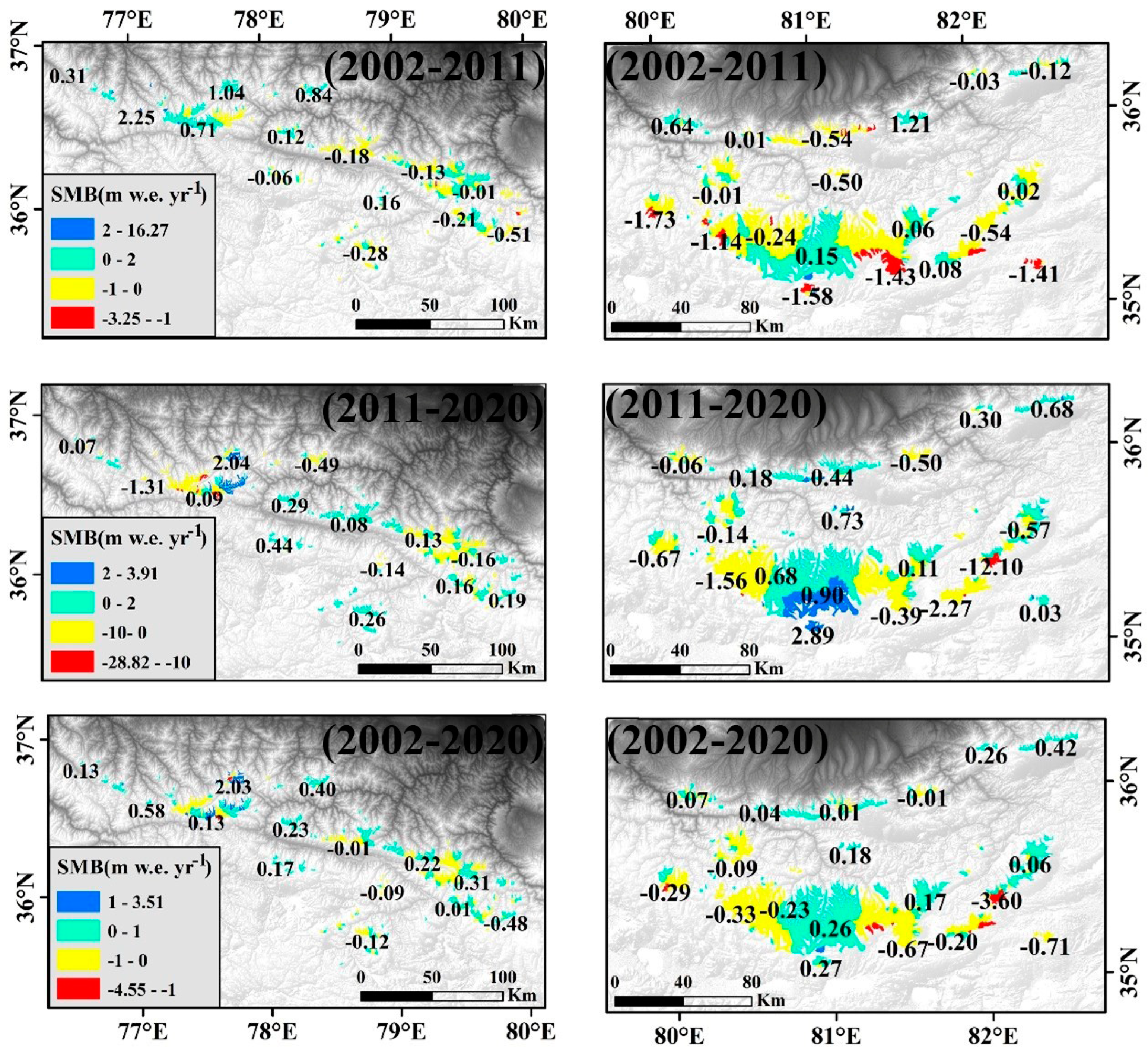
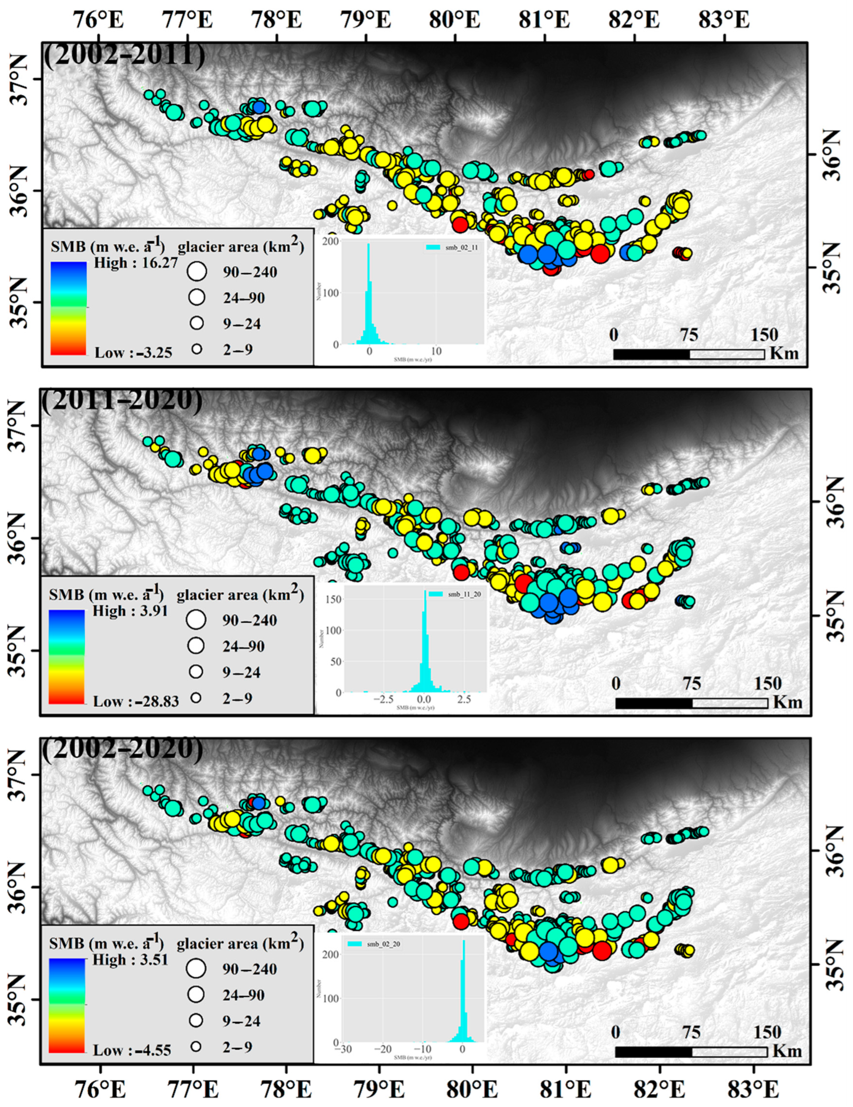
3.1. Varied SMB Spatiotemporal Patterns

In this study, we estimated glacier SMB (>2 km 2 ) in WK (see Figure 3).
We found that during 2002–2011, glacier SMB in eastern WK was 0.05 ± 0.15 m w.e. a 1 , while in western WK, it was 0.20 ± 0.11 m w.e. a 1 , which showed that glaciers were thickening at a higher rate in western WK. From 2011 to 2020, the glacier SMB in western WK was −0.04 ± 0.08 m w.e. a 1 , and in eastern WK it was more negative (−0.16 ± 0.17 m w.e. a 1 ). During 2002–2020, glacier SMB in eastern WK was −0.06 ± 0.07 m w.e. a 1 , while in western WK, it was 0.12   ±   0.06 m w.e. a 1 (see Table 2).
Moreover, according to RGI v6.0, in WK there are 471 and 84 glaciers on the northern and southern slopes, respectively. In western WK, 238 glaciers are located on the northern slope, and 26 glaciers on the southern slope. In eastern WK, there are 233 glaciers on the northern slope and 58 glaciers on the southern slope. We found that in the past two decades, glaciers on the northern slope in eastern WK displayed regular trends of increased gain or reduced loss of ice mass, which is consistent with outcomes obtained by Zhang et al. [79]. However, this trend was reversed in Western WK, except during 2002–2011 (see Table 3).
Overall, glaciers showed different SMB variations between western and eastern WK. Glaciers in western WK predominantly underwent greater gain or reduced loss of ice mass compared with eastern WK. Additionally, we found that there were dissimilar slope effects on SMB distribution in western and eastern WK. The northern slope in western WK showed the greatest loss of mass in the last two decades, while in eastern WK, the southern slope lost more ice mass.
In terms of dissimilar SMB spatial patterns in WK, we found that glacier SMB showed dissimilar variations during different periods. Specifically, during 2002–2011, glacier SMB was 0.10 ± 0.14 m w.e. a 1 , indicating that the glaciers were generally thickening. However, from 2011–2020, glacier SMB showed a slight mass loss (−0.12 ± 0.14 m w.e. a 1 ). During the full period (2002–2020), glacier SMB displayed a slight mass loss in WK (−0.01 ± 0.07 m w.e. a 1 ) (see Figure 4).
Gardner et al. [80] estimated that the average rate of elevation change was 0.17 ± 0.15 m a 1 in WK during 2003–2009, similar to our results (0.18 ± 0.10 m a 1 ). Zhang et al. [79] found that the glacier elevation change was 0.002 ± 0.003 m a 1 in eastern WK during 2000–2018, which also fits our results (−0.01 ± 0.03 m a 1 ). Shean et al. [81] calculated that glacier mass balance in WK was slightly positive (0.01 ± 0.14 m a 1 ) during 2000–2018; the result in ours study was 0.06 ± 0.04 m a 1 during 2002–2020. We also compared glacier elevation change outcomes during 2002–2011 and 2011–2020 with those of Hugonnet et al. [2], which showed only a minor difference, with a maximum dissimilarity of 0.04 m a 1 during 2011–2020. Brun et al. [11] estimated that the glacier mass balance in WK was 0.14 ± 0.08 m w.e. a 1 during 2000–2016, which represents a large difference compared with our results but does overlap within uncertainty. There are two reasons for this difference. First, our time span was 2002–2020, which differed from that studied by Brun et al. [11]. Changes in glacial elevation described by Hugonnet et al. [2] confirmed that glaciers can experience remarkable mass gain or loss with a five-year period. Second, we used the continuity equation rather than the rationally estimated ice density value (850 kg   m 3 ) (see Table 4).

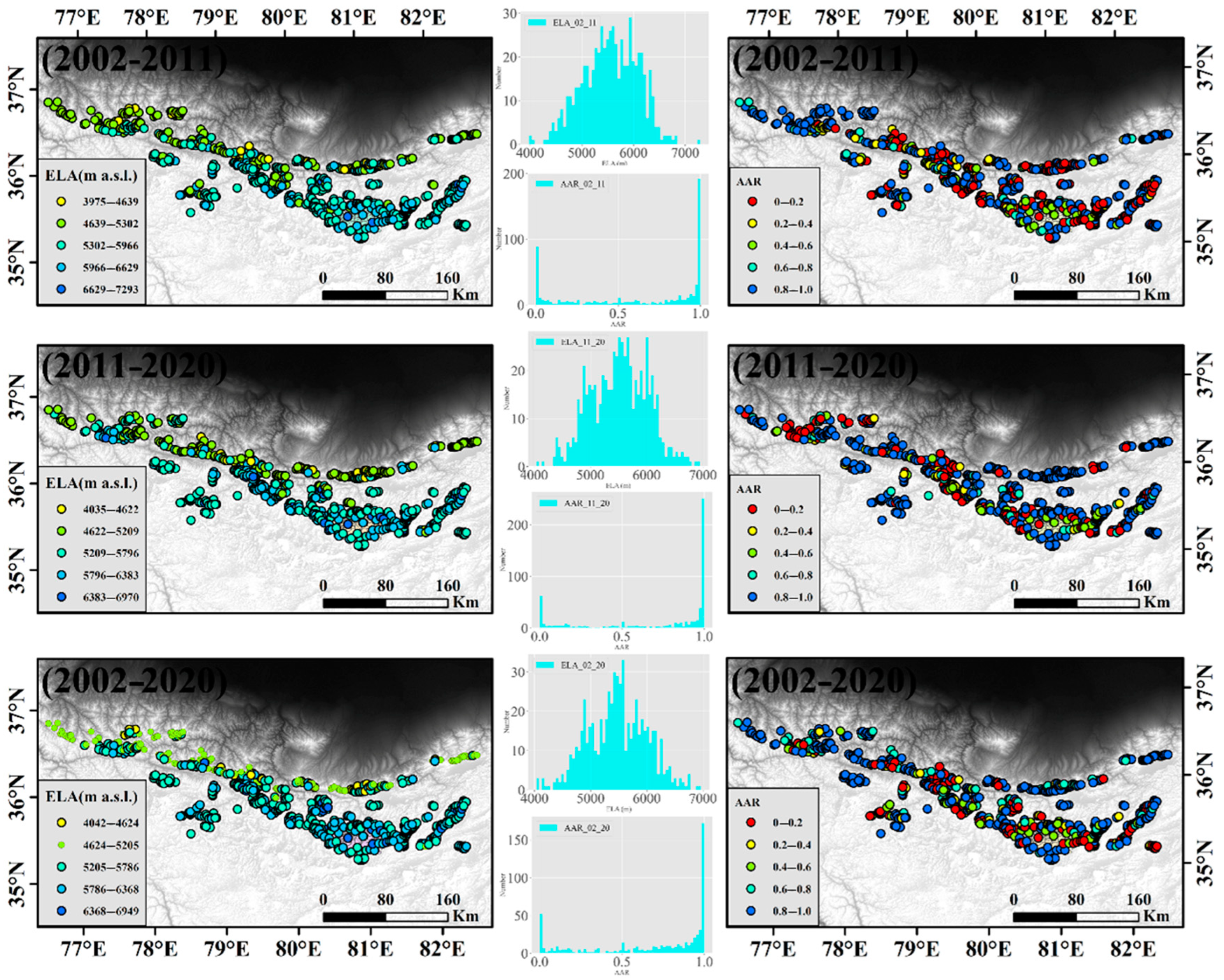
3.2. ELAs and AARs Outcomes

Based on the aforementioned SMB results for three different time spans, we obtained glacier ELAs and AARs across the whole WK. We found that the area-weighted mean and median ELAs in WK from 2002–2020 were 5786 m and 5535 m, respectively, and their respective AARs were 0.58 and 0.78. In HMA, the area-weighted mean and median ELAs and AARs were 5283 m and 5349 m, and 0.51 and 0.44, respectively [23]. This showed that glacier ELAs and AARs (area-weighted mean and medium) in WK were larger than the average levels in HMA (see Figure 5).
Furthermore, in the two subperiods (2002–2011 and 2011–2020), glacier ELAs and AARs showed minor changes. From 2002–2011 and 2011–2020, ELAs were 5788 m and 5744 m, and AARs were 0.59 and 0.62, respectively. We found that ELAs underwent a slight decline and AARs saw a slight increase from the earlier subperiod to the latter, which was inconsistent with the corresponding SMB variations (see Table 5).
Generally speaking, during 2002–2011, 2011–2020, and 2002–2020, glacier ELAs in western WK were always lower and their corresponding AARs were consistently larger than those in eastern WK. We can observe that glacier ELAs increased from 2002–2011 to 2011–2020 in eastern WK, while in western WK, they show an opposite trend.
Owing to the lack of in situ measurements for WK, we were reliant on previous studies to verify our ELA and AAR outcomes [23]. We found that dissimilarities between our results and others were slightly substantial, at 322 m for ELAs and 0.19 for AARs. We assumed that these results were mainly due to different time spans, spatial coverage dissimilarities, glacier samples, and slight differences in the ELA retrieval methods.

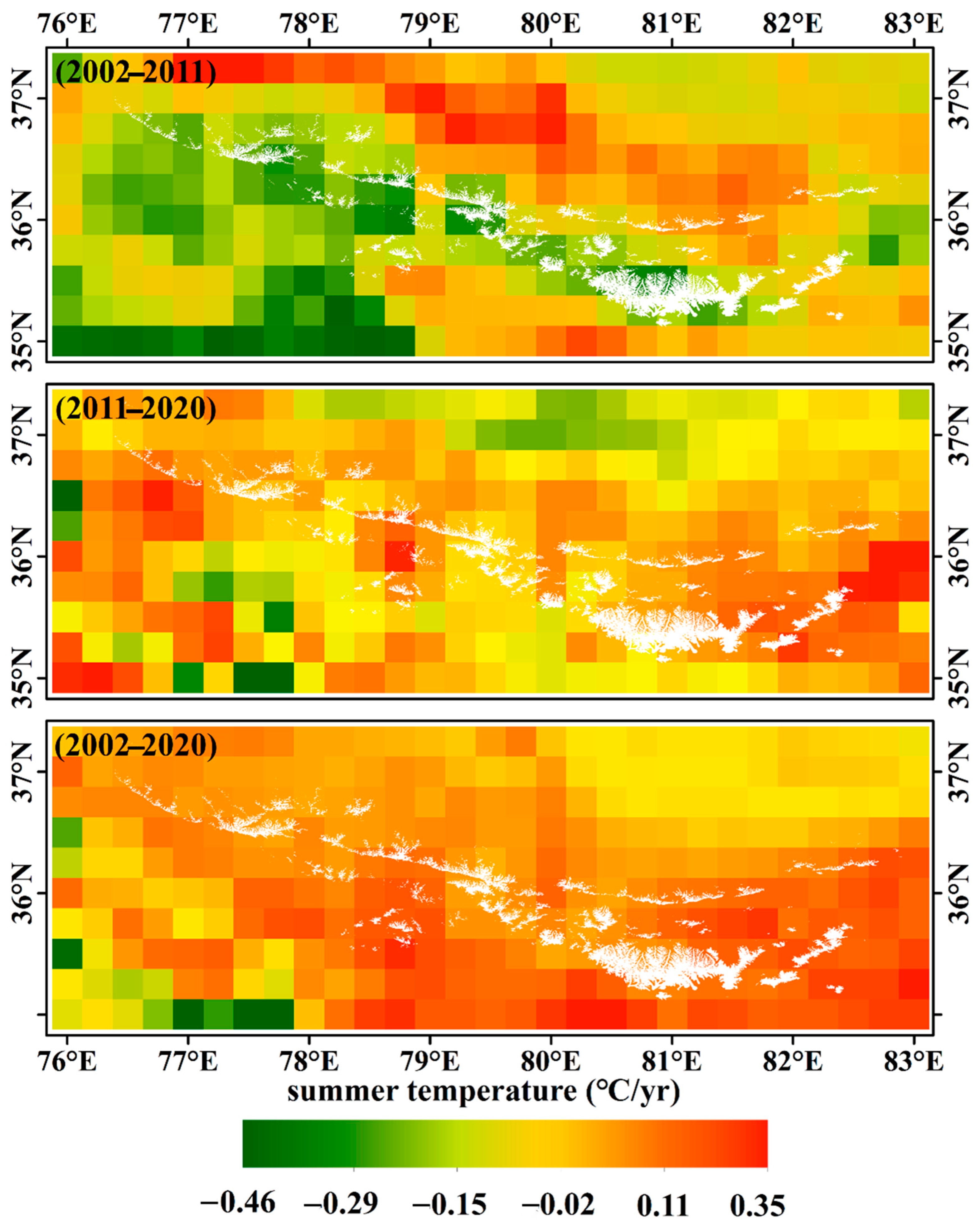
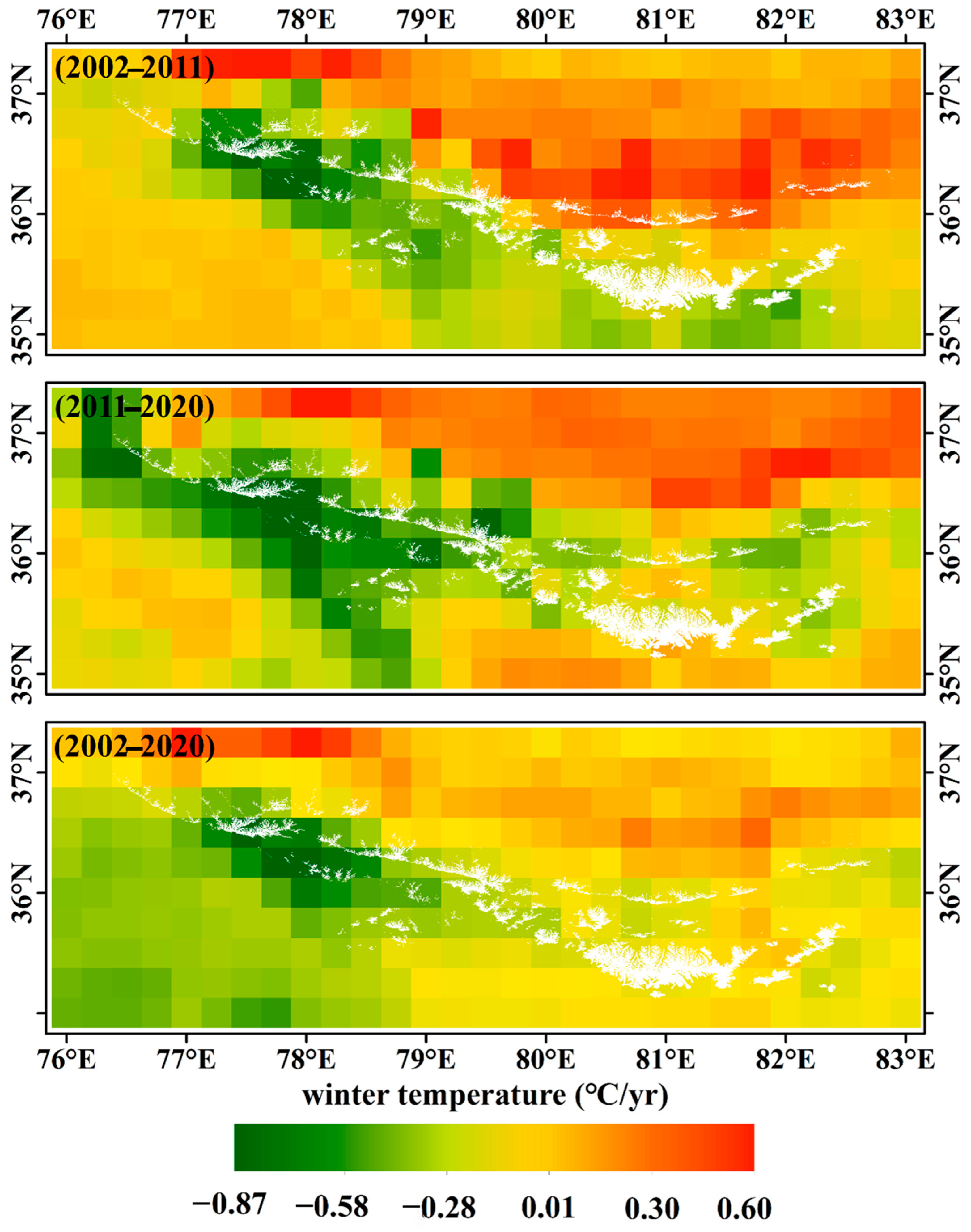
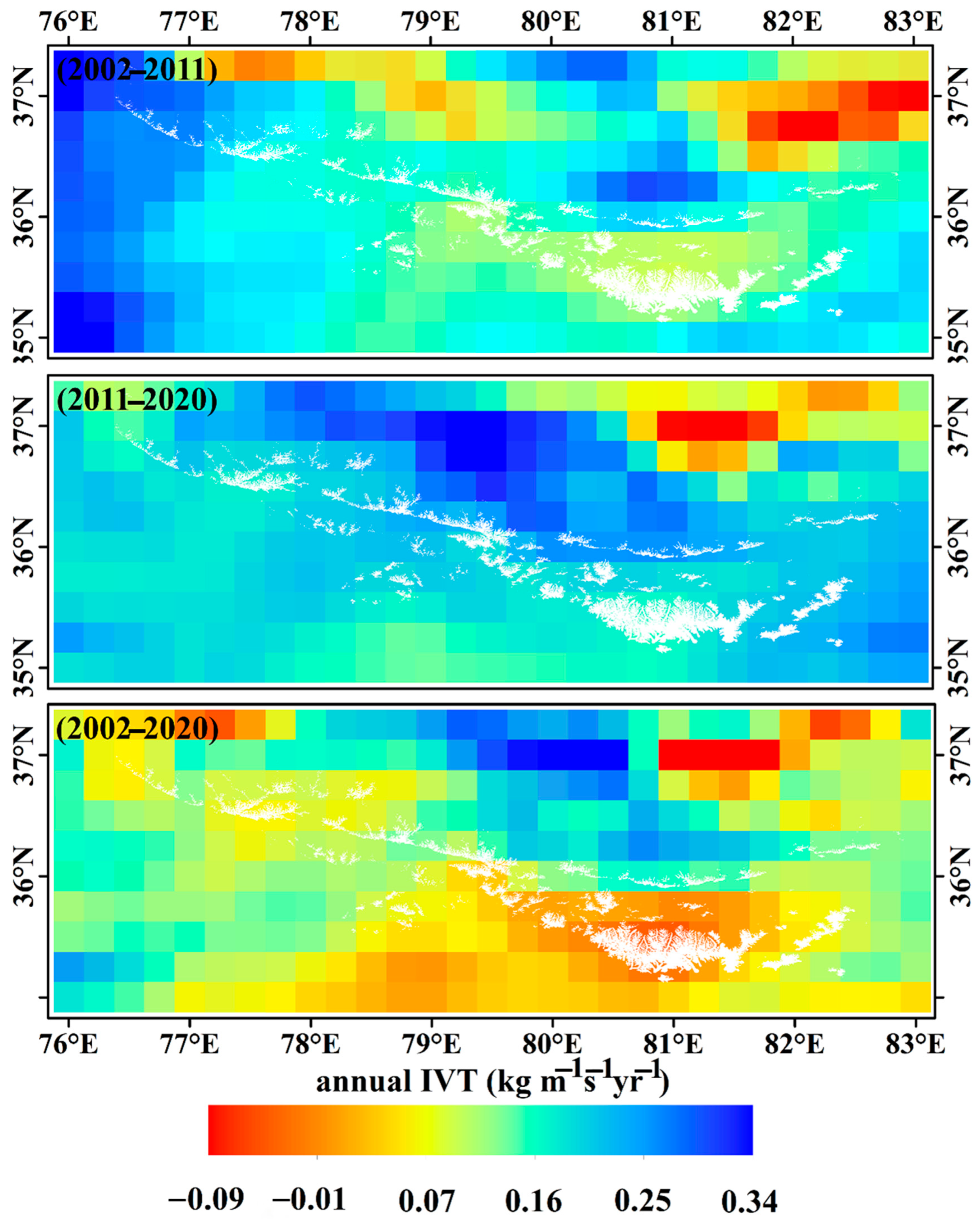
3.3. Skin Temperature and IVT Results

To assess climatic forcing in WK, we extracted the mean annual summer skin temperature (JJA skin temperature), winter skin temperature (December-January-February skin temperature, DJF skin temperature), mean annual IVT, and corresponding summer IVT (JJA IVT) and winter IVT (DJF IVT) trends, for 2002–2011, 2011–2020, and 2002–2020 within the glaciated area [82,83] (the significance and correlation per pixel of climatic factors are described in the Supplementary Information Discussion). Sakai and Fujita [78] assumed that the annual range of monthly temperature (annual temperature) and the ratio of summer IVT have close interplay with glacier mass balance in HMA (Supplementary Information Discussion). However, in this study, we found that the summer IVT ratio and annual skin temperature were less significant than the annual IVT and summer skin temperature when depicting glacier responses to meteorological variations.
Generally speaking, in WK, JJA skin temperature has been increasing, while DJF skin temperature decreased during 2002–2011, 2011–2020, and 2002–2020. In the two subperiods, 2002–2011 and 2011–2020, decreasing JJA skin temperature trends could be observed (from 0.04   a 1 to 0.02   a 1 ), and the DJF skin temperature showed the same tendency (from −0.15   a 1 to −0.25   a 1 ) (see Table 6).
Additionally, during the full period (2002–2020), we found that the JJA skin temperature increased by 0.05   a 1 in western WK, while in eastern WK it increased more obviously (0.08   a 1 ). From 2002–2011, the JJA skin temperature increased by 0.01   a 1 in western WK, while in eastern WK it increased to 0.07   a 1 . During 2011–2020, the JJA skin temperature in western WK maintained the same increasing pace (0.01   a 1 ) as the earlier subperiod, while in eastern WK its rate of increase declined (0.04   a 1 ) (see Figure 6).
Moreover, during 2002–2020, the DJF skin temperature in western WK dropped by 0.09   a 1 , and in eastern WK it declined by 0.01   a 1 . During the earlier subperiod, the DJF skin temperature in western WK decreased by 0.33 °C a 1 , while in eastern WK it increased by 0.02   a 1 . During the later subperiod, the DJF skin temperature decreased by 0.38   a 1 in western WK, while in eastern WK the decrease was −0.15   a 1 , showing a remarkable difference between western and eastern WK (see Figure 7).
Overall, JJA and DJF skin temperatures in western and eastern WK had similar trends during 2011–2020 and 2002–2020, except 2002–2011. Furthermore, across the whole WK, the JJA skin temperature was rising, and the DJF skin temperature was declining.
Additionally, we extracted the annual mean IVT inclination in WK for the last two decades (see Figure 8). The results showed that although IVT inclination in WK continued to rise, the rate of increase was declining. IVT increased at 0.19 kg m 1 s 1   a 1 , 0.16 kg m 1 s 1   a 1 , and 0.10 kg m 1 s 1   a 1 , in 2002–2011, 2011–2020, and 2002–2020, respectively (the IVT direction for the last two decades can be seen in the Supplementary Information Figures).
In two subregions, western WK and eastern WK, there was also an indication that the rate of increase in the annual IVT trend declined from the earlier subperiod (2002–2011) to the later subperiod. In addition, there were almost no differences in the annual IVT trends between western and eastern WK in the three periods (2002–2011, 2011–2020, and 2002–2020) (see Table 7).
Furthermore, we also researched the JJA and DJF IVT trends in WK for the past two decades (see Table 8) (correlation coefficient R and significance p value per pixel are described in Supplementary Information Figures). Overall, we found no obvious spatial differences between western and eastern WK for 2002–2011, 2011–2020, and 2002–2020. Nevertheless, we discovered obvious differences in the JJA and DJF IVT trends between the three periods (2002–2011, 2011–2020, and 2002–2020). Specifically, we found a remarkable increasing JJA IVT trend (0.55 kg m 1 s 1   a 1 ) during 2011–2020, which was apparently higher than the periods 2002–2011 and 2002–2020. In addition, we found that the DJF IVT was decreasing, except during 2011–2020 when it rose by 0.02 kg m 1 s 1   a 1 .

4. Discussion

4.1. Glacial Health in WK

ELAs or AARs can be used to denote the accumulation zone over the glacier surface; thus, they can be used to estimate glacier health in WK. Miles et al. [23] demonstrated that glaciers in WK exhibit much healthier states compared with other HMA regions. Nonetheless, due to limited glacier sample size and the lack of multitemporal comparisons, evidence for glacier well-being in WK remains scarce.
In western WK, we estimate that 69% of glaciers are in a healthy state (regarding glacier healthy state classification here and below, see Section 2.6.2). The remaining unhealthy glaciers show no remarkable thinning pattern, indicating that they are unable to supply much downstream water. In eastern WK, 62% of glaciers are in a healthy state, which demonstrates that glaciers in western WK are healthier and more stable than those in eastern WK. Furthermore, low-quality healthy glaciers account for 84.15% of total glaciers in western WK, while in eastern WK, this figure decreases to 74.72%. This result shows that, when accounting for global warming, western WK exceeds eastern WK in its stores of potential downstream water. We also researched sub-healthy glaciers in WK. The outcomes show that there are 179 glaciers in a state of subhealth in WK. Nonetheless, in contrast to the varied spatial distribution pattern of low-quality healthy glaciers between western WK and eastern WK, the allocation of sub-healthy glaciers is dispersed relatively evenly between the two subregions. The results show that 85 sub-healthy glaciers are located in western WK and 94 glaciers are located in eastern WK.
Additionally, 34 glaciers in WK currently show a superiorly healthy state. The distribution of these glaciers is unevenly dispersed between western and eastern WK; 10 glaciers are located in western WK, and 24 glaciers are located in eastern WK. Furthermore, 15 glaciers are in a supremely unhealthy state in WK, and the number of worst-state glaciers is 14 in eastern WK and one in western WK. Overall, glaciers in eastern WK generally have a more detrimental status and have been the primary downstream water providers for mountain dwellers in the last two decades. However, it will be necessary to pay careful attention to glacier variations in western WK in the upcoming decades, as they hold a substantial quantity of potential meltwater and are more likely to be affected by global warming and become natural hazards [72,84,85,86].
Brun et al. [87] concluded that mean glacier elevation can explain glacier SMB variability for most regions in HMA to some extent (>8%). However, we found no remarkable altitude characteristics in WK that can explain why some glaciers are healthy and others are not. However, we recognize that glacier aspect has some connections with dispersion of glacier well-being in our study area. The results show that 80% of healthy glaciers are on the northern slope, while for unhealthy glaciers, this ratio decreases to 70%. This may contribute to topographic shading effects, altering the potential clear-sky solar radiation received by glaciers [88,89].

4.2. SMB Response to Climate Forcing

Che et al. [40] concluded that the ratios of glacier mass balance to summer skin temperature and precipitation are nonlinear. Wang et al. [90] assumed that sensitivity of glacier mass balance to summer skin temperature is nonlinear, and that the relationship between glacier mass balance and precipitation is linear. Sakai and Fujita [78] assumed a linear mass balance response to both of these climatic factors. However, via deep learning technology, Bolibar et al. [43] suggested that the relationship between glacier mass change and meteorological elements is nonlinear. We compared linear and nonlinear relationships between glacier SMB and climate forcing, using an OLS multilinear regression model and an ANN model, respectively (see Supplementary Information Discussion). Conversely, for extreme positive summer skin temperature changes, the ANN model demonstrated larger glacier SMB sensitivity than the OLS model. For extreme negative summer skin temperature changes, glacier SMB sensitivity was smaller indicated by the ANN model. The results we revealed for the periods 2011–2020 and 2002–2020 match well with Bolibar et al. [43], except for the period 2002–2011.
Generally, both the OLS and ANN models depicted that WK glaciers are more sensitive to IVT than to summer skin temperature in the long run, which may be attributed to the high altitudes of WK glaciers [53,83,90,91]. However, in the two subperiods, glaciers were more sensitive to summer skin temperature.
During 2002–2011, glacier SMB sensitivity to summer skin temperature was −0.38 m w.e./ ; with a 1 increase in summer skin temperature, glacier SMB would decrease 0.38 m w.e. During the period 2011–2020, glacier SMB sensitivity to summer skin temperature was larger (−0.16 m w.e./ ). However, during the full period (2002–2020), glacier SMB sensitivity to summer skin temperature was −0.13 m w.e./ , which was less than in the period 2002–2011. We found that glacier SMB sensitivity to summer skin temperature during 2011–2020 and 2002–2020 was substantially smaller than in other HMA regions [92,93,94,95,96,97]. We believe our results are feasible, because previous studies have shown that glacier SMB sensitivity to summer skin temperature varies in different regions and, generally speaking, continental glaciers are the least sensitive to climate change [90]. Specifically, Ebrahimi and Marshall [98] found that glacier mass balance sensitivity to summer skin temperature was −0.236 m w.e./ in the Canadian Rocky Mountains, which is considerably different from glacier sensitivity to summer skin temperature in Switzerland (−0.63 ~ −0.72 m w.e./ ) [99]. This shows that glaciers in different regions can display different climatic sensitivities, as they are surrounded by varied environmental conditions. Furthermore, glaciers in WK are located at comparatively higher altitudes than other HMA regions, and they are considered continental glaciers; thus, it is reasonable to suggest that their sensitivity to summer skin temperature is smaller than that of glaciers in other HMA regions.
Furthermore, glacier SMB sensitivity to IVT was found to be similar to the summer skin temperature sensitivity pattern. From 2002–2011, glacier SMB sensitivity to IVT was +0.22 m w.e./ kg   m 1 s 1 . Combined with the annual mean IVT during this period, this is equivalent to 0.02 m w.e. ( 50 % ) 1 . This result was smaller than that for its neighbouring region, Karakoram (0.02 m w.e. ( 10 % ) 1 ), and smaller than subcontinental glacier SMB sensitivity to precipitation (0.09 m w.e. ( 10 % ) 1 ) [90]. We believe that a primary reason for this apparent discrepancy is the dissimilar estimation of glacier SMB (Supplementary Information Discussion), as well as the differences between IVT and precipitation [100]. During 2011–2020, glacier SMB sensitivity to IVT was 0.07 m w.e./ kg   m 1 s 1 , equal to approximately 0.01 m w.e. ( 50 % ) 1 . This outcome demonstrated that during the later subperiod, glaciers in WK were less sensitive to IVT than in the earlier subperiod. Overall, during the full time period (2002–2020), glacier SMB sensitivity to IVT was +0.45 m w.e./ kg   m 1 s 1 , which is approximately 0.02 m w.e. ( 50 % ) 1 .

4.3. ELAs Response to Climate Forcing

Sagredo et al. [27] showed that glacier ELA shifts are linearly related to summer skin temperature and precipitation variations. Conversely, motivated by the nonlinear glacier SMB response [43], we researched the nonlinear relationship between glacier ELA shifts and climate forcing (see Supplementary Materials). The result showed that glacier ELA was almost linear with climate change. However, the ANN model captured a significant glacier ELA response to IVT. With the increment of IVT exceeding 0.7 kg m 1 s 1 , the glacier ELA response was less sensitive, and its shift was smaller than the value displayed by the OLS model, indicating that increasing glacier IVT cannot effectively mitigate the impacts of increasing summer skin temperature on variations in glacier ELA. For the following analysis, we exclusively utilized the linear glacier ELA response.
We found that glacier ELA sensitivity was mainly driven by summer skin temperature (+154.66 m/ ) rather than IVT (−121.57 m/ kg   m 1 s 1 ). Zhang et al. [101] found that HMA glaciers are more sensitive to summer skin temperature than to precipitation. Wang et al. [90] concluded that continental glacier ELAs are relatively insensitive to skin temperature change, in contrast with maritime glaciers. The ELA sensitivity of maritime glaciers in HMA is generally +200 ~ 300 m/ , and ELA can sometimes be lifted above the maximum elevation with a merely 1 K increase of summer skin temperature. Furthermore, glacier ELA sensitivity to summer skin temperature varies globally. Noël et al. [102] found that the ELA sensitivity of Svalbard glaciers to summer skin temperature was +129.66 m/ . Sagredo et al. [27] found that Andes glacier ELAs sensitivity to summer skin temperature ranged from +140 ~ 230 m/ . Réveillet et al. [103] found that the ELA sensitivity of the Zongo glacier to summer skin temperature would respond by +120 ~ 180 m/ under different climatic model scenarios. Based on our results, with a 1 increase in summer skin temperature, glacier ELAs in WK would increase 143.76 m, which is reasonable and rational.
Furthermore, Bolibar et al. [43,46] have confirmed that glacier mass change is connected with glacier topography and climatic change. Thus, we can conclude that glacier ELA shift is also connected with these two parameters. However, in the long run, glacier topographic change is comparatively small compared with climatic change, thus, in the current study, we have not accounted for its impact on glacier ELA shift. Based on our retrieved glacier SMB and ELA results, we found that in eastern WK average glacier SMB changed from positive to negative from 2002–2011 to 2011–2020, while glacier ELA decreased in the same period, which is an abnormal phenomenon. We believe that this may be connected with ice flow on the glacier surface. Specifically, if we presume that glaciers are stationary and we ignore the snow drift effect, then the ELA would rise with increasing summer skin temperature. However, the glacier surface velocity in WK is remarkable [47,51,104]; therefore, the ice mass in the accumulation zone would be transferred to lower elevations, which would decrease the ELA. We found that in WK there are 99 glaciers showing negative SMBs and decreasing ELAs. Meanwhile, ice velocity was apparent, and ice flux was positive close to ELA in the accumulation zones of these glaciers. This evidence suggests that the ice mass in the accumulation zone, driven by glacier dynamics, results in the abnormal phenomenon of decreasing ELA. Additionally, this could explain why glacier SMB was negative in the later subperiod (2011–2020), while its corresponding ELA decreased.

5. Conclusions

In this study, we calculated glacier SMB in WK via the continuity equation, for the periods 2002–2011, 2011–2020, and 2002–2020. The results show that in the former time span, glaciers were in a state of mass gain (0.10 ± 0.14 m w.e. a 1 ), while during the later subperiod, glaciers were in a state of mass loss (−0.12 ± 0.14 m w.e. a 1 ). Overall, in the last two decades, glacier SMB in WK has been slightly negative (−0.01 ± 0.07 m w.e. a 1 ). We estimated glacier ELAs and AARs in WK and its two subregions, western and eastern WK, for 2002–2020. We found that ELAs slightly declined from the earlier time span (5788 m) to the later (5744 m), in contrast to SMB variations. We believe that this abnormal phenomenon was due to increasing glacier surface velocities, especially during 2011–2020. We found that glacier surface velocity was apparent in the vicinity of ELAs, and ice flux in the neighboring ELA zones was positive, which could lead to snow or ice slipping over the ELA and amassing in the upper position of the ablation zone. Hence, ELA would decrease, even with increasing summer skin temperature. Furthermore, ELAs in western WK were lower than those in eastern WK, because of the higher median glacier altitude in eastern WK.
Additionally, we found that glaciers in western WK are healthier than those in eastern WK, and that necessary monitoring measurements are still indispensable to safeguard substantially vulnerable low-quality healthy glaciers. Eastern WK glaciers are in a worse state of well-being than western WK glaciers. Furthermore, we established a quantitative relationship between glacier SMB and meteorological elements, summer skin temperature and IVT. The results showed that SMB was mainly affected by summer skin temperature during the two subperiods (2002–2011 and 2011–2020). However, in the full period (2002–2020), glacier SMB was more prone to IVT, which can explain why glacier SMB in WK is less negative than other HMA regions in the last two decades. Overall, glacier SMB was more sensitive to extreme positive summer skin temperatures and less sensitive to extreme negative summer skin temperatures.
Finally, we also observed a quantitative relationship between glacier ELA shifts and the climatic factors of summer skin temperature and IVT. Glacial ELA variations were found to be more sensitive to summer skin temperature (+154.66 m/ ) than to IVT (−121.57 m/ kg   m 1 s 1 ). The ELA shift sensitivity equation has relatively large uncertainty, which could be associated with glacier dynamics. To conclude, the WK glacier ELA is less sensitive to an extremely positive IVT.

Supplementary Materials

The following supporting information can be downloaded at: https://www.mdpi.com/article/10.3390/rs14143465/s1. These materials include supplementary methods, supplementary discussions, supplementary figures, supplementary tables. Supplementary methods introduce the steps of smoothing holes-filled glacier elevation change map. Supplementary discussions mainly describe three parts, comprising the procedures to mosaic multi-temporal ASTER imagery, correlations and significances of meteorological elements trends, and glacier response to climate forcing models (OLS and ANN model). Figure S1: Comparisons between (a) original, (b) inpainting, and (c) smoothing dhdt maps, Figure S2: ASTER DEMs coverage from 2001 to 2005, Figure S3: ASTER DEMs coverage from 2009 to 2013, Figure S4: ASTER DEMs coverage from 2018 to 2021, Figure S5: JJA IVT trend in WK during 2002–2011 (a), 2011–2020 (b), and 2002–2020 (c), Figure S6: DJF IVT trend in WK during 2002–2011 (a), 2011–2020 (b), and 2002–2020 (c), Figure S7: Correlation efficient (Spearman’s R) of JJA skin temperature in WK during 2002–2011 (a), 2011–2020 (b), and 2002–2020 (c), Figure S8: Correlation efficient (Spearman’s R) of DJF surface temperature in WK during (a) 2002–2011, (b) 2011–2020, and (c) 2002–2020, Figure S9: Correlation efficient (Spearman’s R) of annual IVT in WK during (a) 2002–2011, (b) 2011–2020, and (c) 2002–2020, Figure S10: Correlation efficient (Spearman’s R) of JJA IVT in WK during (a) 2002–2011, (b) 2011–2020, and (c) 2002–2020, Figure S11: Correlation efficient (Spearman’s R) of DJF IVT in WK during (a) 2002–2011, (b) 2011–2020, and (c) 2002–2020, Figure S12: Significance (p-value) of JJA surface temperature per pixel in WK during (a) 2002–2011, (b) 2011–2020, and (c) 2002–2020, Figure S13: Significance (p-value) of DJF surface temperature per pixel in WK during (a) 2002–2011, (b) 2011–2020, and (c) 2002–2020, Figure S14: Significance (p-value) of annual IVT per pixel in WK during (a) 2002–2011, (b) 2011–2020, and (c) 2002–2020, Figure S15: Significance (p-value) of JJA IVT per pixel in WK during (a) 2002–2011, (b) 2011–2020, and (c) 2002–2020, Figure S16: Significance (p-value) of DJF IVT per pixel in WK during (a) 2002–2011, (b) 2011–2020, and (c) 2002–2020, Figure S17: Annual IVT trends in WK during (a) 2002–2011, (b) 2011–2020, and (c) 2002–2020, Figure S18: Annual mean surface temperature trend per pixel in WK during (a) 2002–2011, (b) 2011–2020, and (c) 2002–2020, Figure S19: Annual IVT JJA ratio trend per pixel in WK during (a) 2002–2011, (b) 2011–2020, and (c) 2002–2020, Figure S20: Correlation efficient (Spearman’s R) of annual surface temperature per pixel in WK during (a) 2002–2011, (b) 2011–2020, and (c) 2002–2020, Figure S21: Correlation efficient (Spearman’s R) of annual IVT JJA ratio per pixel in WK during (a) 2002–2011, (b) 2011–2020, and (c) 2002–2020, Figure S22: Significance (p-value) of annual mean surface temperature per pixel in WK during (a) 2002–2011, (b) 2011–2020, and (c) 2002–2020, Figure S23: Significance (p-value) of annual JJA IVT ratio per pixel in WK during (a) 2002–2011, (b) 2011–2020, and (c) 2002–2020, Figure S24: Correlation (Spearman’s R) and significance (p-value) between glacier SMB and meteorological factors (JJA surface temperature and annual IVT) in WK during (a) and (b) 2002–2011, (c) and (d) 2011–2020, (e) and (f)2002–2020, Figure S25: Correlation (Spearman’s R) and significance (p-value) between glacier ELAs shift and climatic factors: (a) JJA surface temperature, and (b) annual IVT in WK during 2002–2020, Table S1: The number of ASTER images for different years from 2001–2005. Glacier counts and area (>2 km 2 ) were shielded by ASTER images in each year during this period, Table S2: The number of ASTER imagers for different years from 2009–2013. Glacier counts and area (>2 km 2 ) were shielded by ASTER images in each year during this period, Table S3: The number of ASTER images for different years from 2018–2021. Glacier counts and area (>2 km 2 ) were shielded by ASTER images in each year during this period, Table S4: Correlation coefficients (R) and significances (p-value) between glacier mass balance and climatic factors (JJA surface temperature and annual IVT) for three periods (2002–2011, 2011–2020, and 2002–2020), Table S5: Correlation coefficient (R) and significance (p-value) between glacier ELAs shifts and climatic factors (JJA surface temperature and annual IVT) during the period 2002–2020.

Author Contributions

Conceptualization, C.-Q.K.; Data curation, J.L.; Formal analysis, J.L.; Funding acquisition, C.-Q.K.; Validation, T.S.; Writing-original draft, J.L.; Writing-review and editing, T.S. All authors have read and agreed to the published version of the manuscript.

Funding

This work is supported by the Program for National Natural Science Foundation of China (Grant No. 41830105).

Data Availability Statement

The ASTER imagery was obtained from Earthdata (https://earthdata.nasa.gov/, accessed on 23 April 2022). The glacier velocity dataset was provided by NASA MEaSUREs ITS_LIVE project (https://its-live.jpl.nasa.gov/, accessed on 23 April 2022). the glacier thickness dataset is available at https://doi.org/10.3929/ethz-b-000315707, accessed on 23 April 2022. The RGI v6.0 dataset is available at https://www.glims.org/RGI/rgi60_dl.html, accessed on 23 April 2022. The supraglacial debris extents are available at https://zenodo.org/record/3866466#.YYOuu21By00, accessed on 23 April 2022. The HydroLAKES v1.0 dataset is available at https://www.hydrosheds.org/page/hydrolakes, accessed on 23 April 2022. The glacial lakes dataset is available at https://nsidc.org/data/HMA_GLI/versions/1, accessed on 23 April 2022. The ERA 5.1 reanalysis datasets were provided by EVMWF and can be downloaded at this website: https://www.ecmwf.int/en/forecasts/datasets/reanalysis-datasets/era5, accessed on 23 April 2022. The DEM co-registration code is from Github: https://github.com/dshean/demcoreg, accessed on 23 April 2022.

Acknowledgments

We thank Evan S. Miles for his guidance in the original manuscript.

Conflicts of Interest

The authors declare no conflict of interest.

Acronyms

AcronymDefinition
AAR(s)Glacier accumulation area zone(s)
ANN modelArtificial neural network model
ASTERAdvanced Spaceborne Thermal Emission and Reflection Radiometer
DJFMonth from December to next year’s February
ELA(s)Glacier equilibrium line altitude(s)
GH indexGlacier health index
GECGlacier elevation change
HMAHigh Mountain Asia
IVTIntegrated water vapor transport
JJAMonth from June to August
OLS modelOrdinary least square model
RGI v6.0Randolph Glacier Inventory version 6.0
SMBSpecific mass balance
SRTM DEMShuttle Radar Topography Mission Digital Elevation Model
WKWest Kunlun Mountains

References

  1. Zemp, M.; Huss, M.; Thibert, E.; Eckert, N.; McNabb, R.W.; Huber, J.; Barandun, M.; Machguth, H.; Nussbaumer, S.U.; Gärtner-Roer, I.; et al. Global glacier mass changes and their contributions to sea-level rise from 1961 to 2016. Nature 2019, 568, 382–386. [Google Scholar] [CrossRef]
  2. Hugonnet, R.; McNabb, R.; Berthier, E.; Menounos, B.; Nuth, C.; Girod, L.; Farinotti, D.; Huss, M.; Dussaillant, I.; Brun, F.; et al. Accelerated global glacier mass loss in the early twenty-first century. Nature 2021, 592, 726–731. [Google Scholar] [CrossRef] [PubMed]
  3. Vörösmarty, C.J.; McIntyre, P.B.; Gessner, M.O.; Dudgeon, D.; Prusevich, A.; Green, P.; Glidden, S.; Bunn, S.E.; Sullivan, C.A.; Liermann, C.R.; et al. Global threats to human water security and river biodiversity. Nature 2010, 467, 555–561. [Google Scholar] [CrossRef] [PubMed]
  4. Pörtner, H.O.; Roberts, D.C.; Masson-Delmotte, V.; Zhai, P.; Tignor, M.; Poloczanska, E.; Mintenbeck, K.; Alegría, A.; Nicolai, M.; Okem, A.; et al. The ocean and cryosphere in a changing climate. In IPCC Special Report on the Ocean and Cryosphere in a Changing Climate; Cambridge University Press: Cambridge, UK; New York, NY, USA, 2019. [Google Scholar]
  5. IPCC. Summary for Policymakers. In Climate Change 2013: The Physical Science Basis. Contribution of Working Group I to the Fifth Assessment Report of the Intergovernmental Panel on Climate Change; Stocker, T.F., Qin, D., Plattner, G.-K., Tignor, M., Allen, S.K., Boschung, J., Nauels, A., Xia, Y., Bex, V., Midgley, P.M., Eds.; Cambridge University Press: Cambridge, UK; New York, NY, USA, 2013. [Google Scholar]
  6. Farinotti, D.; Huss, M.; Fürst, J.J.; Landmann, J.M.; Machguth, H.; Maussion, F.; Pandit, A. A consensus estimate for the ice thickness distribution of all glaciers on Earth. Nat. Geosci. 2019, 12, 168–173. [Google Scholar] [CrossRef] [Green Version]
  7. Pfeffer, W.T.; Arendt, A.A.; Bliss, A.; Bolch, T.; Bolch, J.G.; Gardner, A.S.; Hagen, J.-O.; Hock, R.; Kaser, G.; Kienholz, C.; et al. The Randolph Glacier Inventory: A globally complete inventory of glaciers. J. Glaciol. 2014, 60, 537–552. [Google Scholar] [CrossRef] [Green Version]
  8. RGI Consortium. Randolph Glacier Inventory-A Dataset of Global Glacier Outlines, Version 6; NSIDC, National Snow and Ice Data Center: Boulder, CO, USA, 2017. [Google Scholar] [CrossRef]
  9. Kraaijenbrink, P.D.A.; Bierkens, M.F.P.; Lutz, A.F.; Immerzeel, W.W. Impact of a global temperature rise of 1.5 degrees Celsius on Asia’s glaciers. Nature 2017, 549, 257–260. [Google Scholar] [CrossRef]
  10. Hewitt, K. The Karakoram anomaly? Glacier expansion and the ‘elevation effect, ’Karakoram Himalaya. Mt. Res. Dev. 2005, 25, 332–340. [Google Scholar] [CrossRef] [Green Version]
  11. Brun, F.; Berthier, E.; Wagnon, P.; Kääb, A.; Treichler, D. A spatially resolved estimate of High Mountain Asia glacier mass balances from 2000 to 2016. Nat. Geosci. 2017, 10, 668–673. [Google Scholar] [CrossRef] [Green Version]
  12. Bashir, F.; Zeng, X.; Gupta, H.; Hazenberg, P. A hydrometeorological perspective on the Karakoram anomaly using unique valley-based synoptic weather observations. Geophys. Res. Lett. 2017, 44, 10470–10478. [Google Scholar] [CrossRef] [Green Version]
  13. Berthier, E.; Brun, F. Karakoram geodetic glacier mass balances between 2008 and 2016: Persistence of the anomaly and influence of a large rock avalanche on Siachen Glacier. J. Glaciol. 2019, 65, 494–507. [Google Scholar] [CrossRef] [Green Version]
  14. Farinotti, D.; Immerzeel, W.W.; de Kok, R.J.; Quincey, D.J.; Dehecq, A. Manifestations and mechanisms of the Karakoram glacier Anomaly. Nat. Geosci. 2020, 13, 8–16. [Google Scholar] [CrossRef] [PubMed]
  15. Wang, Q.; Yi, S.; Sun, W. Continuous estimates of glacier mass balance in high mountain Asia based on ICESat-1, 2 and GRACE/GRACE follow-on data. Geophys. Res. Lett. 2021, 48, e2020GL090954. [Google Scholar] [CrossRef]
  16. Kääb, A.; Treichler, D.; Nuth, C.; Berthier, E. Brief Communication: Contending estimates of 2003–2008 glacier mass balance over the Pamir–Karakoram–Himalaya. Cryosphere 2015, 9, 557–564. [Google Scholar] [CrossRef] [Green Version]
  17. Liang, Q.; Wang, N.; Yang, X.; Chen, A.; Hua, T.; Li, Z.; Yang, D. The eastern limit of ‘Kunlun-Pamir-Karakoram Anomaly’reflected by changes in glacier area and surface elevation. J. Glaciol. 2022, 1–10. [Google Scholar] [CrossRef]
  18. Wang, Y.; Hou, S.; Huai, B.; An, W.; Pang, H.; Liu, Y. Glacier anomaly over the western Kunlun Mountains, Northwestern Tibetan Plateau, since the 1970s. J. Glaciol. 2018, 64, 624–636. [Google Scholar] [CrossRef] [Green Version]
  19. Neckel, N.; Kropáček, J.; Bolch, T.; Hochschild, V. Glacier mass changes on the Tibetan Plateau 2003–2009 derived from ICESat laser altimetry measurements. Environ. Res. Lett. 2014, 9, 014009. [Google Scholar] [CrossRef]
  20. Lin, H.; Li, G.; Cuo, L.; Ye, Q. A decreasing glacier mass balance gradient from the edge of the Upper Tarim Basin to the Karakoram during 2000–2014. Sci. Rep. 2017, 7, 6712. [Google Scholar] [CrossRef]
  21. Cao, B.; Guan, W.; Li, K.; Wen, Z.; Han, H.; Pan, B. Area and Mass Changes of Glaciers in the West Kunlun Mountains Based on the Analysis of Multi-Temporal Remote Sensing Images and DEMs from 1970 to 2018. Remote Sens. 2020, 12, 2632. [Google Scholar] [CrossRef]
  22. Huss, M. Density assumptions for converting geodetic glacier volume change to mass change. Cryosphere 2013, 7, 877–887. [Google Scholar] [CrossRef] [Green Version]
  23. Miles, E.; McCarthy, M.; Dehecq, A.; Kneib, M.; Fugger, S.; Pellicciotti, F. Health and sustainability of glaciers in High Mountain Asia. Nat. Commun. 2021, 12, 2868. [Google Scholar] [CrossRef]
  24. Benn, D.I.; Lehmkuhl, F. Mass balance and equilibrium-line altitudes of glaciers in high-mountain environments. Quat. Int. 2000, 65, 15–29. [Google Scholar] [CrossRef]
  25. Braithwaite, R.J.; Raper, S.C.B. Estimating equilibrium-line altitude (ELA) from glacier inventory data. Ann. Glaciol. 2009, 50, 127–132. [Google Scholar] [CrossRef] [Green Version]
  26. Pellitero, R.; Rea, B.R.; Spagnolo, M.; Bakke, J.; Hughes, P.; Ivy-Ochs, S.; Lukas, S.; Ribolini, A. A GIS tool for automatic calculation of glacier equilibrium-line altitudes. Comput. Geosci. 2015, 82, 55–62. [Google Scholar] [CrossRef]
  27. Sagredo, E.A.; Rupper, S.; Lowell, T.V. Sensitivities of the equilibrium line altitude to temperature and precipitation changes along the Andes. Quat. Res. 2014, 81, 355–366. [Google Scholar] [CrossRef]
  28. Stuart-Smith, R.F.; Roe, G.H.; Li, S.; Allen, M.R. Increased outburst flood hazard from Lake Palcacocha due to human-induced glacier retreat. Nat. Geosci. 2021, 14, 85–90. [Google Scholar] [CrossRef]
  29. Kurowski, L. Die Höhe der Schneegrenze mit Besonderer Berücksichtigung der Finsteraarhorn-Gruppe, Pencks Geographische Abhandlungen 5; Nabu Press: Berlin, Germany, 1891; pp. 119–160. [Google Scholar]
  30. Osmaston, H.A. The Past and Present Climate and Vegetation of Ruwenzori and Its Neighbourhood. Ph.D. Thesis, University of Oxford, Oxford, UK, 1965. [Google Scholar]
  31. Osmaston, H. Estimates of glacier equilibrium line altitudes by the Area × Altitude, the Area × Altitude Balance Ratio and the Area × Altitude Balance Index methods and their validation. Quat. Int. 2005, 138, 22–31. [Google Scholar] [CrossRef]
  32. Rabatel, A.; Letréguilly, A.; Dedieu, J.P.; Eckert, N. Changes in glacier equilibrium-line altitude in the western Alps from 1984 to 2010: Evaluation by remote sensing and modeling of the morpho-topographic and climate controls. Cryosphere 2013, 7, 1455–1471. [Google Scholar] [CrossRef] [Green Version]
  33. Barandun, M.; Pohl, E.; Naegeli, K.; McNabb, R.; Huss, M.; Berthier, E.; Saks, T.; Hoelzle, M. Hot spots of glacier mass balance variability in Central Asia. Geophys. Res. Lett. 2021, 48, e2020GL092084. [Google Scholar] [CrossRef]
  34. Herreid, S.; Pellicciotti, F. The state of rock debris covering Earth’s glaciers. Nat. Geosci. 2020, 13, 621–627. [Google Scholar] [CrossRef]
  35. De Would, M.; Hock, R. Static mass-balance sensitivity of Arctic glaciers and ice caps using a degree-day approach. Ann. Glaciol. 2005, 42, 217–224. [Google Scholar]
  36. Fujita, K. Effect of precipitation seasonality on climatic sensitivity of glacier mass balance. Earth Planet. Sci. Lett. 2008, 276, 14–19. [Google Scholar] [CrossRef]
  37. Fujita, K. Influence of precipitation seasonality on glacier mass balance and its sensitivity to climate change. Ann. Glaciol. 2008, 48, 88–92. [Google Scholar] [CrossRef] [Green Version]
  38. Anderson, B.; Mackintosh, A. Controls on mass balance sensitivity of maritime glaciers in the Southern Alps, New Zealand: The role of debris cover. J. Geophys. Res. Earth Surf. 2012, 117. [Google Scholar] [CrossRef]
  39. Engelhardt, M.; Schuler, T.V.; Andreassen, L.M. Sensitivities of glacier mass balance and runoff to climate perturbations in Norway. Ann. Glaciol. 2015, 56, 79–88. [Google Scholar] [CrossRef] [Green Version]
  40. Che, Y.; Zhang, M.; Li, Z.; Wei, Y.; Nan, Z.; Li, H.; Wang, S.; Su, B. Energy balance model of mass balance and its sensitivity to meteorological variability on Urumqi River Glacier No. 1 in the Chinese Tien Shan. Sci. Rep. 2019, 9, 13958. [Google Scholar] [CrossRef] [Green Version]
  41. Kinnard, C.; Larouche, O.; Demuth, M.N.; Menounos, B. Mass balance modelling and climate sensitivity of Saskatchewan Glacier, western Canada. Cryosphere Discuss. 2021, 1–38. [Google Scholar] [CrossRef]
  42. Naegeli, K.; Huss, M. Sensitivity of mountain glacier mass balance to changes in bare-ice albedo. Ann. Glaciol. 2017, 58 Pt 2, 119–129. [Google Scholar] [CrossRef] [Green Version]
  43. Bolibar, J.; Rabatel, A.; Gouttevin, I.; Zekollari, H.; Galiez, C. Nonlinear sensitivity of glacier mass balance to future climate change unveiled by deep learning. Nat. Commun. 2022, 13, 409. [Google Scholar] [CrossRef] [PubMed]
  44. Caidong, C.; Sorteberg, A. Modelled mass balance of Xibu glacier, Tibetan Plateau: Sensitivity to climate change. J. Glaciol. 2010, 56, 235–248. [Google Scholar] [CrossRef] [Green Version]
  45. McGrath, D.; Sass, L.; O’Neel, S.; Arendt, A.; Kienholz, C. Hypsometric control on glacier mass balance sensitivity in Alaska and northwest Canada. Earth’s Future 2017, 5, 324–336. [Google Scholar] [CrossRef] [Green Version]
  46. Bolibar, J.; Rabatel, A.; Gouttevin, I.; Galiez, C.; Condom, T.; Sauquet, E. Deep learning applied to glacier evolution modelling. Cryosphere 2020, 14, 565–584. [Google Scholar] [CrossRef] [Green Version]
  47. Dehecq, A.; Gourmelen, N.; Gardner, A.S.; Brun, F.; Goldberg, D.; Nienow, P.W.; Berthier, E.; Vincent, C.; Wagnon, P.; Trouvé, E. Twenty-first century glacier slowdown driven by mass loss in High Mountain Asia. Nat. Geosci. 2019, 12, 22–27. [Google Scholar] [CrossRef]
  48. Hersbach, H.; Bell, B.; Berrisford, P.; Hirahara, S.; Horányi, A.; Muñoz-Sabater, J.; Nicolas, J.; Peubey, C.; Radu, R.; Schepers, D.; et al. The ERA5 global reanalysis. Q. J. R. Meteorol. Soc. 2020, 146, 1999–2049. [Google Scholar] [CrossRef]
  49. Yao, T.D.; Jiao, K.Q.; Zhang, X.P.; Zhang, Y.; Thompson, L.G. Glaciologic studies on Guliya ice cap. J. Glaciol. Geocryol. 1992, 14, 233–241. [Google Scholar]
  50. Shangguan, D.; Liu, S.; Ding, Y.; Li, J.; Zhang, Y.; Ding, L.; Wang, X.; Xie, C.; Li, G. Glacier changes in the west Kunlun Shan from 1970 to 2001 derived from Landsat TM/ETM+ and Chinese glacier inventory data. Ann. Glaciol. 2007, 46, 204–208. [Google Scholar] [CrossRef] [Green Version]
  51. Yasuda, T.; Furuya, M. Dynamics of surge-type glaciers in West Kunlun Shan, northwestern Tibet. J. Geophys. Res. Earth Surf. 2015, 120, 2393–2405. [Google Scholar] [CrossRef] [Green Version]
  52. Zheng, B.; Fushimi, H.; Jiao, K.; Li, S.J. Characteristics of basal till and the discovery of tephra layers in the West Kunlun Mountains. Bull. Glacier Res. 1989, 7, 177–186. [Google Scholar]
  53. Maussion, F.; Scherer, D.; Mölg, T.; Collier, E.; Curio, J.; Finkelnburg, R. Precipitation seasonality and variability over the Tibetan Plateau as resolved by the High Asia Reanalysis. J. Clim. 2014, 27, 1910–1927. [Google Scholar] [CrossRef] [Green Version]
  54. Berthier, E.; Schiefer, E.; Clarke, G.K.C.; Menounos, B.; Remy, F. Contribution of Alaskan glaciers to sea-level rise derived from satellite imagery. Nat. Geosci. 2010, 3, 92–95. [Google Scholar] [CrossRef] [Green Version]
  55. Ohmura, A. Observed mass balance of mountain glaciers and Greenland ice sheet in the 20th century and the present trends. Surv. Geophys. 2011, 32, 537–554. [Google Scholar] [CrossRef]
  56. Gardelle, J.; Berthier, E.; Arnaud, Y.; Kääb, A. Region-wide glacier mass balances over the Pamir-Karakoram-Himalaya during 1999–2011. Cryosphere 2013, 7, 1263–1286. [Google Scholar] [CrossRef] [Green Version]
  57. Girod, L.; Nuth, C.; Kääb, A.; McNabb, R.; Galland, O. MMASTER: Improved ASTER DEMs for elevation change monitoring. Remote Sens. 2017, 9, 704. [Google Scholar] [CrossRef] [Green Version]
  58. Nuth, C.; Kääb, A. Co-registration and bias corrections of satellite elevation data sets for quantifying glacier thickness change. Cryosphere 2011, 5, 271–290. [Google Scholar] [CrossRef] [Green Version]
  59. Gardelle, J.; Berthier, E.; Arnaud, Y. Impact of resolution and radar penetration on glacier elevation changes computed from DEM differencing. J. Glaciol. 2012, 58, 419–422. [Google Scholar] [CrossRef] [Green Version]
  60. Höhle, J.; Höhle, M. Accuracy assessment of digital elevation models by means of robust statistical methods. ISPRS J. Photogramm. Remote Sens. 2009, 64, 398–406. [Google Scholar] [CrossRef] [Green Version]
  61. Dussaillant, I.; Berthier, E.; Brun, F.; Masiokas, M.; Hugonnet, R.; Favier, V.; Rabatel, A.; Pitte, P.; Ruiz, L. Two decades of glacier mass loss along the Andes. Nat. Geosci. 2019, 12, 802–808. [Google Scholar] [CrossRef]
  62. Hubbard, A.; Willis, I.; Sharp, M.; Mair, D.; Nienow, P.; Hubbard, B.; Blatter, H. Glacier mass-balance determination by remote sensing and high-resolution modelling. J. Glaciol. 2000, 46, 491–498. [Google Scholar] [CrossRef] [Green Version]
  63. Berthier, E.; Vincent, C. Relative contribution of surface mass-balance and ice-flux changes to the accelerated thinning of Mer de Glace, French Alps, over1979–2008. J. Glaciol. 2012, 58, 501–512. [Google Scholar] [CrossRef] [Green Version]
  64. Van Tricht, L.; Huybrechts, P.; Van Breedam, J.; Vanhulle, A.; Van Oost, K.; Zekollari, H. Estimating surface mass balance patterns from unoccupied aerial vehicle measurements in the ablation area of the Morteratsch–Pers glacier complex (Switzerland). Cryosphere 2021, 15, 4445–4464. [Google Scholar] [CrossRef]
  65. Kaser, G.; Fountain, A.; Jansson, P. A Manual for Monitoring the Mass Balance of Mountain Glaciers; UNESCO: Paris, France, 2003. [Google Scholar]
  66. Huss, M.; Dhulst, L.; Bauder, A. New long-term mass-balance series for the Swiss Alps. J. Glaciol. 2015, 61, 551–562. [Google Scholar] [CrossRef] [Green Version]
  67. Cuffey, K.M.; Paterson WS, B. The Physics of Glaciers; Academic Press: Cambridge, MA, USA, 2010. [Google Scholar]
  68. Shumskiy, P.A. Density of glacier ice. J. Glaciol. 1960, 3, 568–573. [Google Scholar] [CrossRef] [Green Version]
  69. McNabb, R.; Nuth, C.; Kääb, A.; Girod, L. Sensitivity of glacier volume change estimation to DEM void interpolation. Cryosphere 2019, 13, 895–910. [Google Scholar] [CrossRef] [Green Version]
  70. Seehaus, T.; Malz, P.; Sommer, C.; Lippl, S.; Cochachin, A.; Braun, M. Changes of the tropical glaciers throughout Peru between 2000 and 2016–mass balance and area fluctuations. Cryosphere 2019, 13, 2537–2556. [Google Scholar] [CrossRef] [Green Version]
  71. Seehaus, T.; Malz, P.; Sommer, C.; Soruco, A.; Rabatel, A.; Braun, M.H. Mass balance and area changes of glaciers in the Cordillera Real and Tres Cruces, Bolivia, between 2000 and 2016. J. Glaciol. 2020, 66, 124–136. [Google Scholar] [CrossRef] [Green Version]
  72. Messager, M.L.; Lehner, B.; Grill, G.; Nedeva, I.; Schmitt, O. Estimating the volume and age of water stored in global lakes using a geo-statistical approach. Nat. Commun. 2016, 7, 13603. [Google Scholar] [CrossRef]
  73. Shugar, D.H.; Burr, A.; Haritashya, U.K.; Kargel, J.S.; Watson, C.S.; Kennedy, M.C.; Bevington, A.R.; Betts, R.A.; Harrison, S.; Strattman, K. Rapid worldwide growth of glacial lakes since 1990. Nat. Clim. Chang. 2020, 10, 939–945. [Google Scholar] [CrossRef]
  74. Huang, L.; Li, Z.; Zhou, J.M.; Zhang, P. An automatic method for clean glacier and nonseasonal snow area change estimation in High Mountain Asia from 1990 to 2018. Remote Sens. Environ. 2021, 258, 112376. [Google Scholar] [CrossRef]
  75. Seehaus, T.; Morgenshtern, V.; Hübner, F.; Bänsch, E.; Braun, M. Novel techniques for void filling in glacier elevation change data sets. Remote Sens. 2020, 12, 3917. [Google Scholar] [CrossRef]
  76. Rabatel, A.; Dedieu, J.P.; Vincent, C. Using remote-sensing data to determine equilibrium-line altitude and mass-balance time series: Validation on three French glaciers, 1994–2002. J. Glaciol. 2005, 51, 539–546. [Google Scholar] [CrossRef] [Green Version]
  77. Dice, L.R. Measures of the amount of ecologic association between species. Ecology 1945, 26, 297–302. [Google Scholar] [CrossRef]
  78. Sakai, A.; Fujita, K. Contrasting glacier responses to recent climate change in high-mountain Asia. Sci. Rep. 2017, 7, 13717. [Google Scholar] [CrossRef] [PubMed]
  79. Zhang, G.; Chen, W.; Li, G.; Yang, W.; Yi, S.; Luo, W. Lake water and glacier mass gains in the northwestern Tibetan Plateau observed from multi-sensor remote sensing data: Implication of an enhanced hydrological cycle. Remote Sens. Environ. 2020, 237, 111554. [Google Scholar] [CrossRef]
  80. Gardner, A.S.; Moholdt, G.; Cogley, J.G.; Wouters, B.; Arendt, A.A.; Wahr, J.; Berthier, E.; Hock, R.; Pfeffer, W.T.; Kaser, G.; et al. A reconciled estimate of glacier contributions to sea level rise: 2003 to 2009. Science 2013, 340, 852–857. [Google Scholar] [CrossRef] [Green Version]
  81. Shean, D.E.; Bhushan, S.; Montesano, P.; Rounce, D.R.; Arendt, A.; Osmanoglu, B. A systematic, regional assessment of high mountain Asia glacier mass balance. Front. Earth Sci. 2020, 7, 363. [Google Scholar] [CrossRef] [Green Version]
  82. Mattingly, K.S.; Mote, T.L.; Fettweis, X. Atmospheric river impacts on Greenland Ice Sheet surface mass balance. J. Geophys. Res. Atmos. 2018, 123, 8538–8560. [Google Scholar] [CrossRef] [Green Version]
  83. Braun, M.H.; Malz, P.; Sommer, C.; Farías-Barahona, D.; Sauter, T.; Casassa, G.; Soruco, A.; Skvarca, P.; Seehaus, T.C. Constraining glacier elevation and mass changes in South America. Nat. Clim. Chang. 2019, 9, 130–136. [Google Scholar] [CrossRef]
  84. Kirschbaum, D.; Kapnick, S.B.; Stanley, T.; Pascale, S. Changes in extreme precipitation and landslides over high mountain Asia. Geophys. Res. Lett. 2020, 47, e2019GL085347. [Google Scholar] [CrossRef]
  85. Liu, J.; Wu, Y.; Gao, X. Increase in occurrence of large glacier-related landslides in the high mountains of Asia. Sci. Rep. 2021, 11, 1635. [Google Scholar] [CrossRef]
  86. Nie, Y.; Pritchard, H.D.; Liu, Q.; Hennig, T.; Wang, W.; Wang, X.; Liu, S.; Nepal, S.; Samyn, D.; Hewitt, K.; et al. Glacial change and hydrological implications in the Himalaya and Karakoram. Nat. Rev. Earth Environ. 2021, 2, 91–106. [Google Scholar] [CrossRef]
  87. Brun, F.; Wagnon, P.; Berthier, E.; Jomelli, V.; Maharjan, S.B.; Shrestha, F.; Kraaijenbrink, P. Heterogeneous influence of glacier morphology on the mass balance variability in High Mountain Asia. J. Geophys. Res. Earth Surf. 2019, 124, 1331–1345. [Google Scholar] [CrossRef]
  88. Arnold, N.S.; Rees, W.G.; Hodson, A.J.; Kohler, J. Topographic controls on the surface energy balance of a high Arctic valley glacier. J. Geophys. Res. Earth Surf. 2006, 111. [Google Scholar] [CrossRef]
  89. Olson, M.; Rupper, S. Impacts of topographic shading on direct solar radiation for valley glaciers in complex topography. Cryosphere 2019, 13, 29–40. [Google Scholar] [CrossRef] [Green Version]
  90. Wang, R.; Liu, S.; Shangguan, D.; Radić, V.; Zhang, Y. Spatial heterogeneity in glacier mass-balance sensitivity across High Mountain Asia. Water 2019, 11, 776. [Google Scholar] [CrossRef] [Green Version]
  91. Yao, T.D.; Thompson, L.; Yang, W.; Yu, W.S.; Gao, Y.; Guo, X.J.; Yang, X.X.; Duan, K.Q.; Zhao, H.B.; Xu, B.Q.; et al. Different glacier status with atmospheric circulations in Tibetan Plateau and surroundings. Nat. Clim. Chang. 2012, 2, 663–667. [Google Scholar] [CrossRef]
  92. Liu, S.; Xie, Z.; Wang, N.; Ye, B. Mass balance sensitivity to climate change: A case study of Glacier No. 1 at Urumqi Riverhead, Tianshan Mountains, China. Chin. Geogr. Sci. 1999, 9, 134–140. [Google Scholar] [CrossRef]
  93. Jiang, X.; Wang, N.L.; He, J.Q.; Wu, X.; Song, G. A distributed surface energy and mass balance model and its application to a mountain glacier in China. Chin. Sci. Bull. 2010, 55, 2079–2087. [Google Scholar] [CrossRef]
  94. Wang, S.; Pu, J.; Wang, N. Study on mass balance and sensitivity to climate change in summer on the Qiyi Glacier, Qilian Mountains. Sci. Cold Arid Reg. 2012, 4, 281–287. [Google Scholar]
  95. Rasmussen, L.A. Meteorological controls on glacier mass balance in High Asia. Ann. Glaciol. 2013, 54, 352–359. [Google Scholar] [CrossRef] [Green Version]
  96. Sun, W.; Qin, X.; Wang, Y.; Chen, J.; Du, W.; Zhang, T.; Huai, B. The response of surface mass and energy balance of a continental glacier to climate variability, western Qilian Mountains, China. Clim. Dyn. 2018, 50, 3557–3570. [Google Scholar] [CrossRef]
  97. Zhu, M.; Yao, T.; Yang, W.; Xu, B.; Wu, G.; Wang, X. Differences in mass balance behavior for three glaciers from different climatic regions on the Tibetan Plateau. Clim. Dyn. 2018, 50, 3457–3484. [Google Scholar] [CrossRef]
  98. Ebrahimi, S.; Marshall, S.J. Surface energy balance sensitivity to meteorological variability on Haig Glacier, Canadian Rocky Mountains. Cryosphere 2016, 10, 2799–2819. [Google Scholar] [CrossRef] [Green Version]
  99. Huss, M.; Fischer, M. Sensitivity of very small glaciers in the Swiss Alps to future climate change. Front. Earth Sci. 2016, 4, 34. [Google Scholar] [CrossRef] [Green Version]
  100. Makama, E.K.; Lim, H.S. Variability and Trend in Integrated Water Vapour from ERA-Interim and IGRA2 Observations over Peninsular Malaysia. Atmosphere 2020, 11, 1012. [Google Scholar] [CrossRef]
  101. Zhang, Y.; Fujita, K.; Ageta, Y.; Nakawo, M. The response of glacier ELA to climate fluctuations on High-Asia. Bull. Glacier Res. 1998, 16, 1–11. [Google Scholar]
  102. Noël, B.; Jakobs, C.L.; Van Pelt, W.J.J.; Lhermitte, S.; Wouters, B.; Kohler, J.; Hagen, J.O.; Luks, B.; Reijmer, C.H.; van de Berg, W.J.; et al. Low elevation of Svalbard glaciers drives high mass loss variability. Nat. Commun. 2020, 11, 4597. [Google Scholar] [CrossRef] [PubMed]
  103. Réveillet, M.; Rabatel, A.; Gillet-Chaulet, F.; Soruco, A. Simulations of changes to Glaciar Zongo, Bolivia (16 S), over the 21st century using a 3-D full-Stokes model and CMIP5 climate projections. Ann. Glaciol. 2015, 56, 89–97. [Google Scholar] [CrossRef] [Green Version]
  104. Yasuda, T.; Furuya, M. Short-term glacier velocity changes at West Kunlun Shan, Northwest Tibet, detected by synthetic aperture radar data. Remote Sens. Environ. 2013, 128, 87–106. [Google Scholar] [CrossRef] [Green Version]
Figure 1. Overview of the study area. Sub panel: Locations of study area, West Kunlun (WK), in High Mountain Asia (HMA). Main panel: Location of glaciers in the WK and outlines of Advanced Spaceborne Thermal Emission and Reflection Radiometer (ASTER) coverage used in this study, including subdivision in Western WK and Eastern WK. Background image is Shuttle Radar Topography Mission Digital Elevation Model (SRTM DEM). We used Randolph Glacier Inventory version 6.0 (RGI v6.0) as the glacier outline.
Remotesensing 14 03465 g001
Figure 2. One sampled ASTER DEM for 2002, showing the DEM difference (a) before and (b) after co-registration; (c) is the statistical analysis of this process (in the subplot (c), med indicates median, and NMAD is normalized median absolute deviation).
Remotesensing 14 03465 g002
Figure 3. Glacier SMB spatial pattern differences in western WK (in the left three subplots) and eastern WK (in the right three subplots) in the past two decades.
Remotesensing 14 03465 g003
Figure 4. Glacier SMB temporal alterations in WK during 2002–2011, 2011–2020, and 2002–2020.
Remotesensing 14 03465 g004
Figure 5. Equilibrium line altitudes (ELAs) (left three subplots) and accumulation area ratios (AARs) (right three subplots) for each glacier in WK for three different periods; 2002–2011, 2011–2020, and 2002–2020.
Remotesensing 14 03465 g005
Figure 6. Annual JJA skin temperature trends in WK for 2002–2011, 2011–2020, and 2002–2020, derived from ERA5.1.
Remotesensing 14 03465 g006
Figure 7. Annual DJF skin temperature trends in WK for 2002–2011, 2011–2020, and 2002–2020, derived from ERA5.1.
Remotesensing 14 03465 g007
Figure 8. Annual mean integrated water vapor transport (IVT) trends in WK for 2002–2011, 2011–2020, and 2002–2020, derived from ERA5.1.
Remotesensing 14 03465 g008
Table 1. Data used in this study to calculate glacier specific mass balance (SMB).
Data UsedTimeSpatial Resolution (m)NumberPurpose
ASTER L1A2001–20201587Glacier SMB
ITS_LIVE2001–202024019Mean ice velocity
* Farinotti et al., 20192000–201625615Ice thickness estimation
ERA 5.12002–20200.25° × 0.25°-Climatic analysis
* Ice thickness data set from https://www.research-collection.ethz.ch/handle/20.500.11850/315707, accessed on 23 April 2022.
Table 2. Spatial variations of SMB in WK over three different time spans. (unit: m w.e. a 1 ).
PeriodsWestern WKEastern WKWK
2002–20110.20 ± 0.110.05 ± 0.150.10 ± 0.14
2011–2020−0.04 ± 0.08−0.16 ± 0.17−0.12 ± 0.14
2002–20200.12 ± 0.06−0.06 ± 0.07−0.01 ± 0.07
Table 3. Spatial variations of glacier SMB in northern and southern slopes of WK and its two subregions over three different time spans. (unit: m w.e. a 1 ).
PeriodsNorthern SlopeSouthern Slope
Western WKEastern WKWKWestern WKEastern WKWK
2002–20110.09 ± 0.10−0.47 ± 0.14−0.28 ± 0.131.02 ± 0.190.77 ± 0.170.79 ± 0.17
2011–20200.14 ± 0.080.19 ± 0.160.17 ± 0.13−0.47 ± 0.090.26 ± 0.170.22 ± 0.17
2002–20200.20 ± 0.050.01 ± 0.070.07 ± 0.06−0.14 ± 0.110.09 ± 0.080.08 ± 0.08
Table 4. Averaged glacier elevation change (GEC), in a unit of m a 1 , comparing our results and others.
PeriodsRegionGECStudyNotes of Methods
2003–2009WK0.17 ± 0.15Gardner et al. [80]ICESat
2000–2010WK0.19 ± 0.12Hugonnet et al. [2]ASTER
2010–2020WK−0.05 ± 0.11Hugonnet et al. [2]ASTER
2000–2016WK0.18 ± 0.33Brun et al. [11]ASTER
2000–2018Eastern WK0.002 ± 0.003Zhang et al. [79]SRTM and TanDEM-X
2000–2018WK0.01 ± 0.14Shean et al. [81]WorldView-1/2/3, GeoEye-1, and ASTER
2000–2020WK0.08 ± 0.07Hugonnet et al. [2]ASTER
Table 5. Median and area-weighted mean ELAs (unit: m a.s.l.) and AARs in WK and its two subregions, during 2002–2011, 2011–2020, and 2002–2020 (the former are area-weighted mean ELAs or AARs, and the latter are median ELAs or AARs).
PeriodsELAsAARs
Western WKEastern WKWKWestern WKEastern WKWK
2002–20115381/53795965/57325788/55700.67/0.670.50/0.760.59/0.76
2011–20205510/54065846/55195744/54820.55/0.640.64/0.900.62/0.81
2002–20205451/53675932/56245786/55350.60/0.670.54/0.840.58/0.78
Table 6. June-July-August (JJA) and December-January-February (DJF) skin temperature (unit:   a 1 ) trends in western WK, eastern WK and WK overall, over three time periods.
PeriodsJJA Skin TemperatureDJF Skin Temperature
Western WKEastern WKWKWestern WKEastern WKWK
2002–20110.010.070.04−0.330.02−0.15
2011–20200.010.040.02−0.38−0.15−0.25
2002–20200.050.080.06−0.09−0.01−0.04
Table 7. Annual IVT (unit: kg m 1 s 1   a 1 ) trends in Western WK, Eastern WK and WK over three periods.
PeriodWestern WKEastern WKWK
2002–20110.200.180.19
2011–20200.160.160.16
2002–20200.100.100.10
Table 8. JJA and DJF IVT trends (unit: kg m 1 s 1   a 1 ) in western WK, eastern WK, and WK during three different periods.
PeriodsJJA IVT TrendDJF IVT Trend
Western WKEastern WKWKWestern WKEastern WKWK
2002–20110.330.300.32−0.17−0.10−0.14
2011–20200.570.530.550.030.010.02
2002–20200.260.260.26−0.10−0.06−0.08
Publisher’s Note: MDPI stays neutral with regard to jurisdictional claims in published maps and institutional affiliations.

