
An Efficient User-Friendly Integration Tool for Landslide Susceptibility Mapping Based on Support Vector Machines: SVM-LSM Toolbox

 ,
,  ,
,
Abstract
:1. Introduction
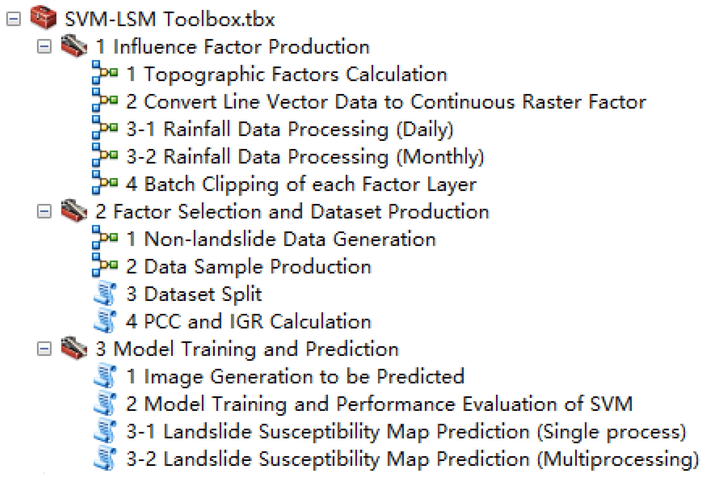
2. LSM Toolbox
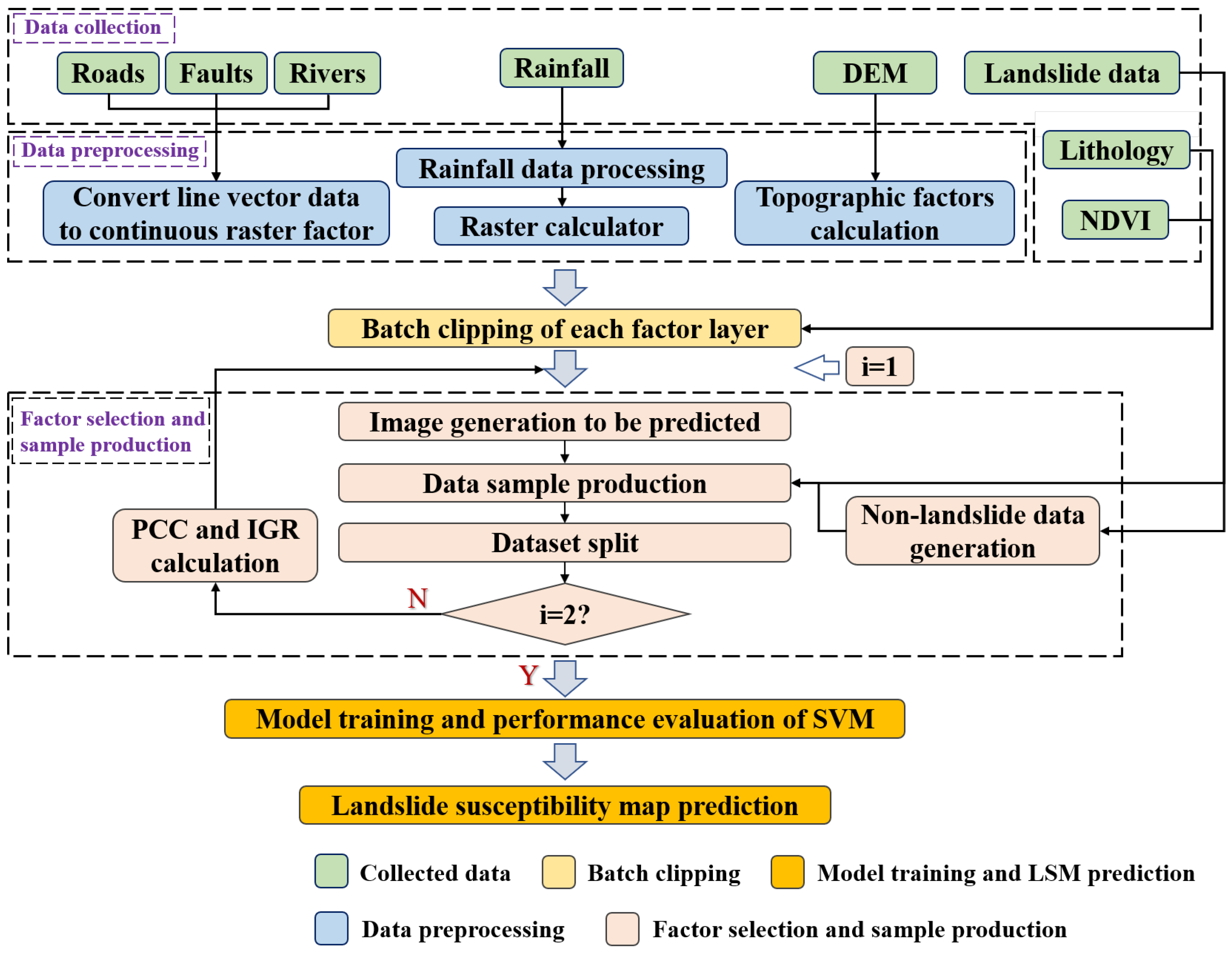
2.1. LSM Workflow
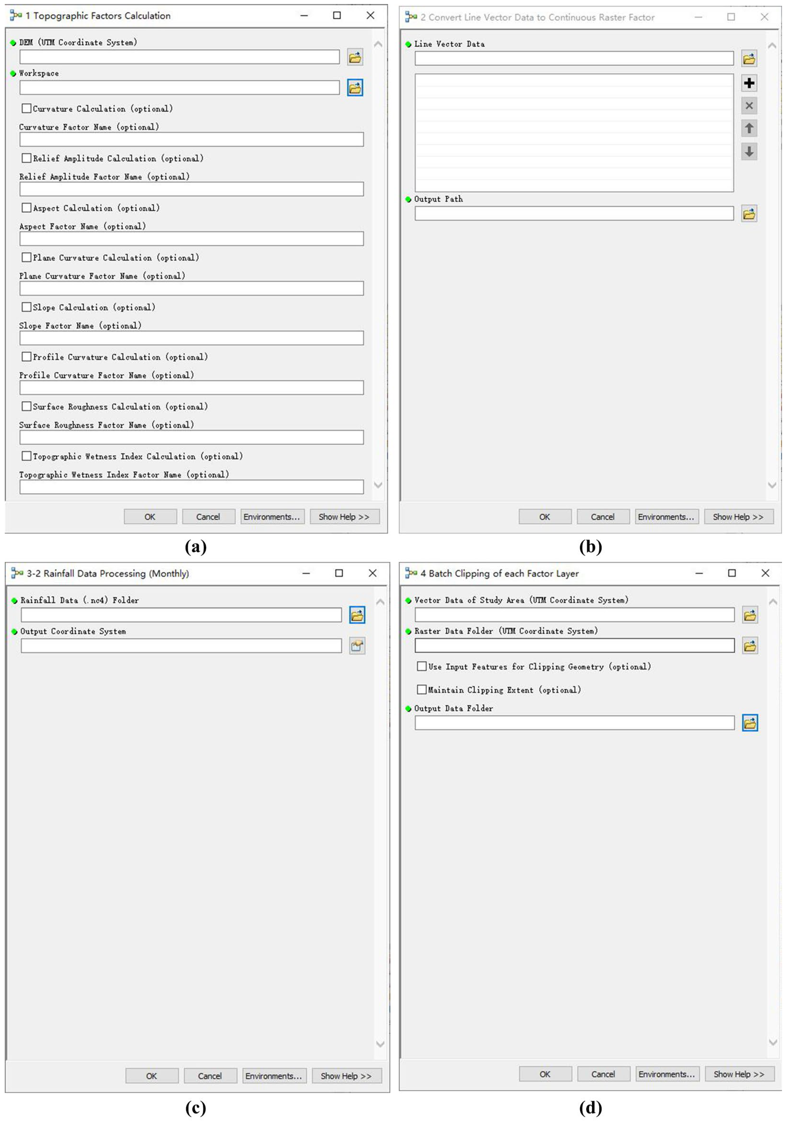
2.2. Influencing Factor Production
2.2.1. Topographic Factor Calculation
2.2.2. Convert Line Vector Data to Continuous Raster Factor
2.2.3. Rainfall Data Processing
2.2.4. Batch Clipping of Each Factor Layer
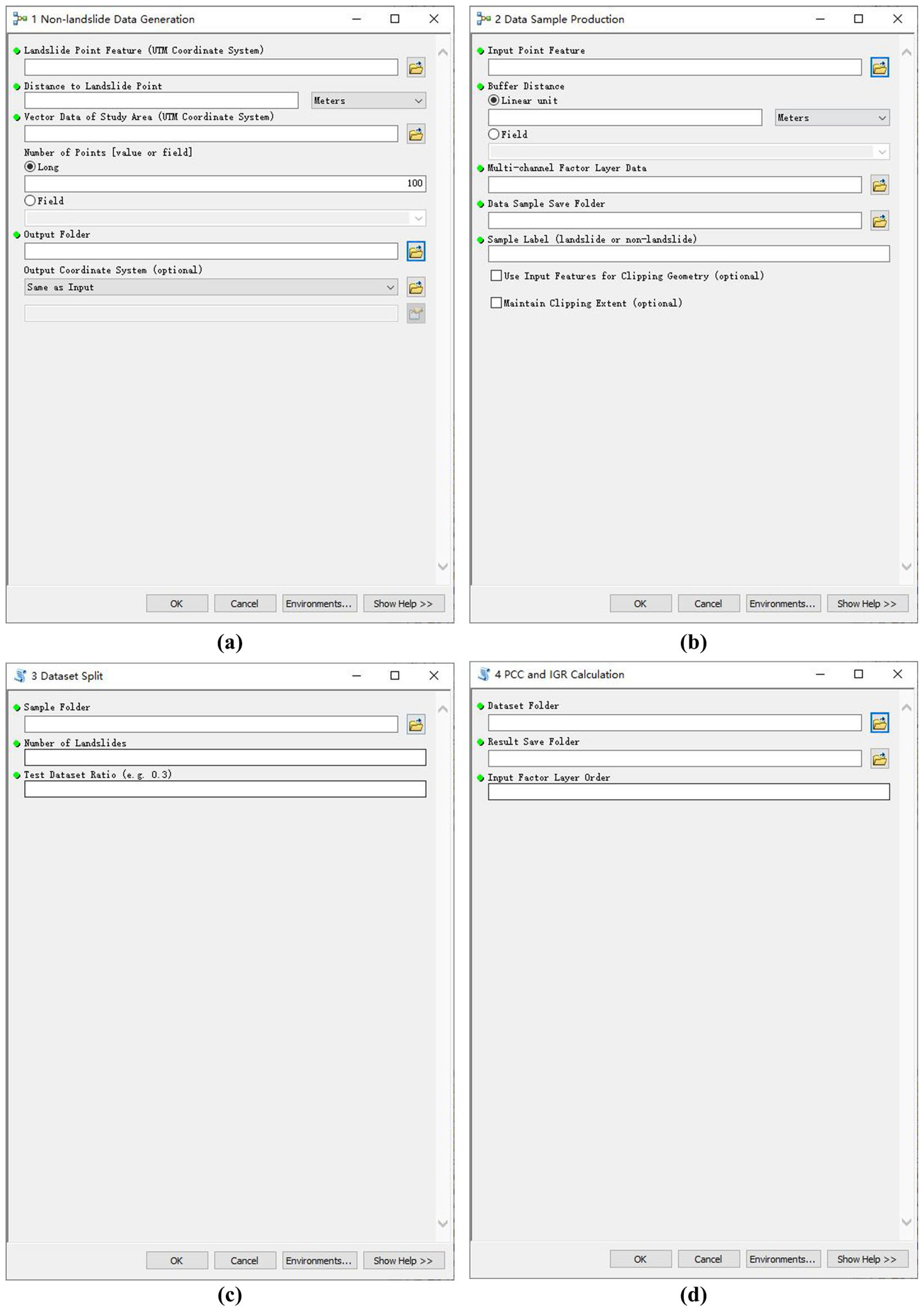
2.3. Factor Selection and Dataset Production
2.3.1. Non-Landslide Data Generation
2.3.2. Data Sample Production
2.3.3. Dataset Split
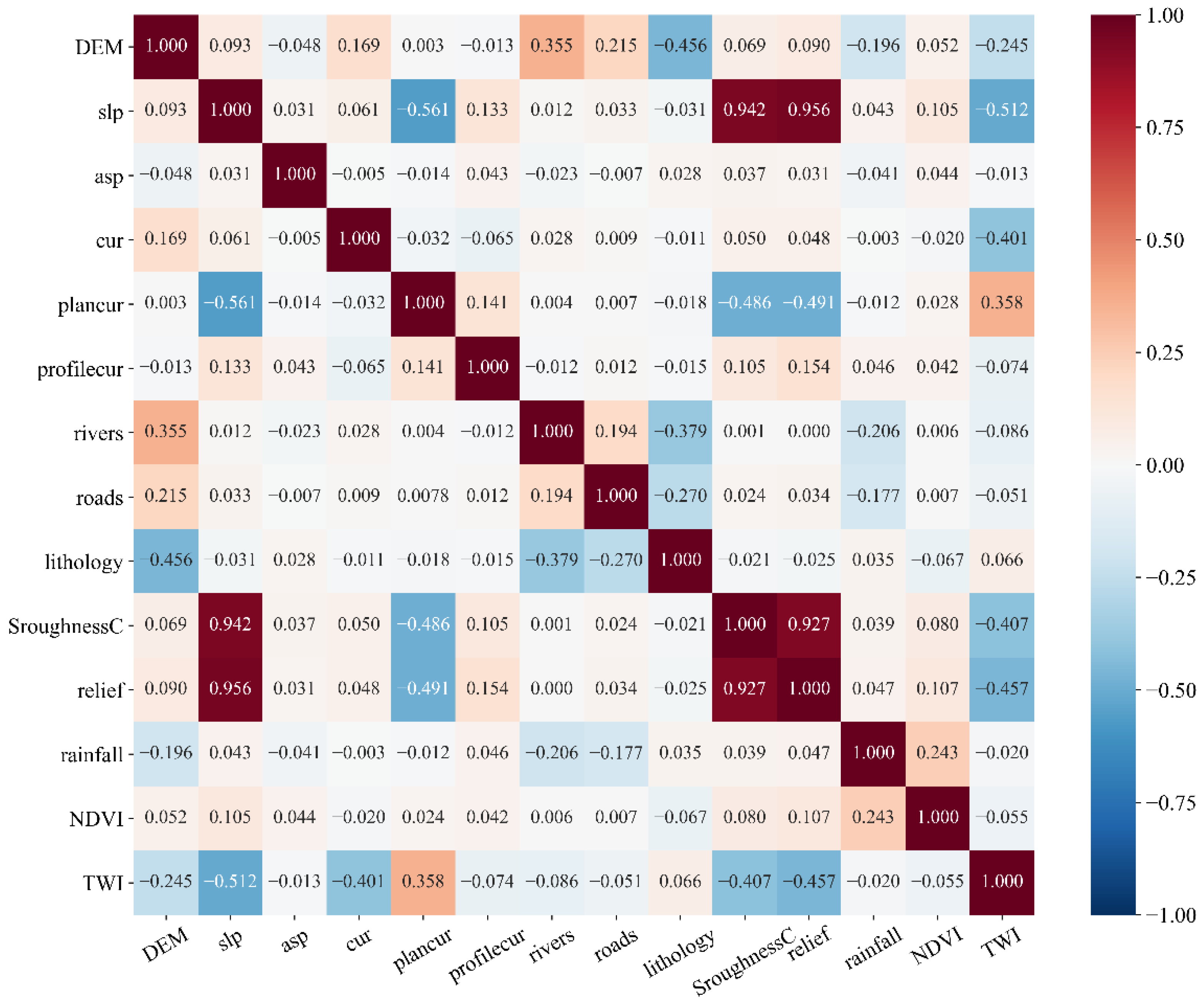
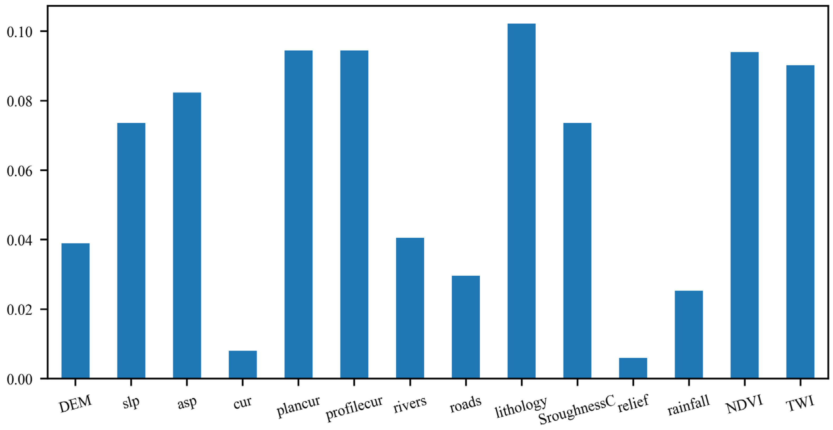
2.3.4. PCC and IGR Calculation
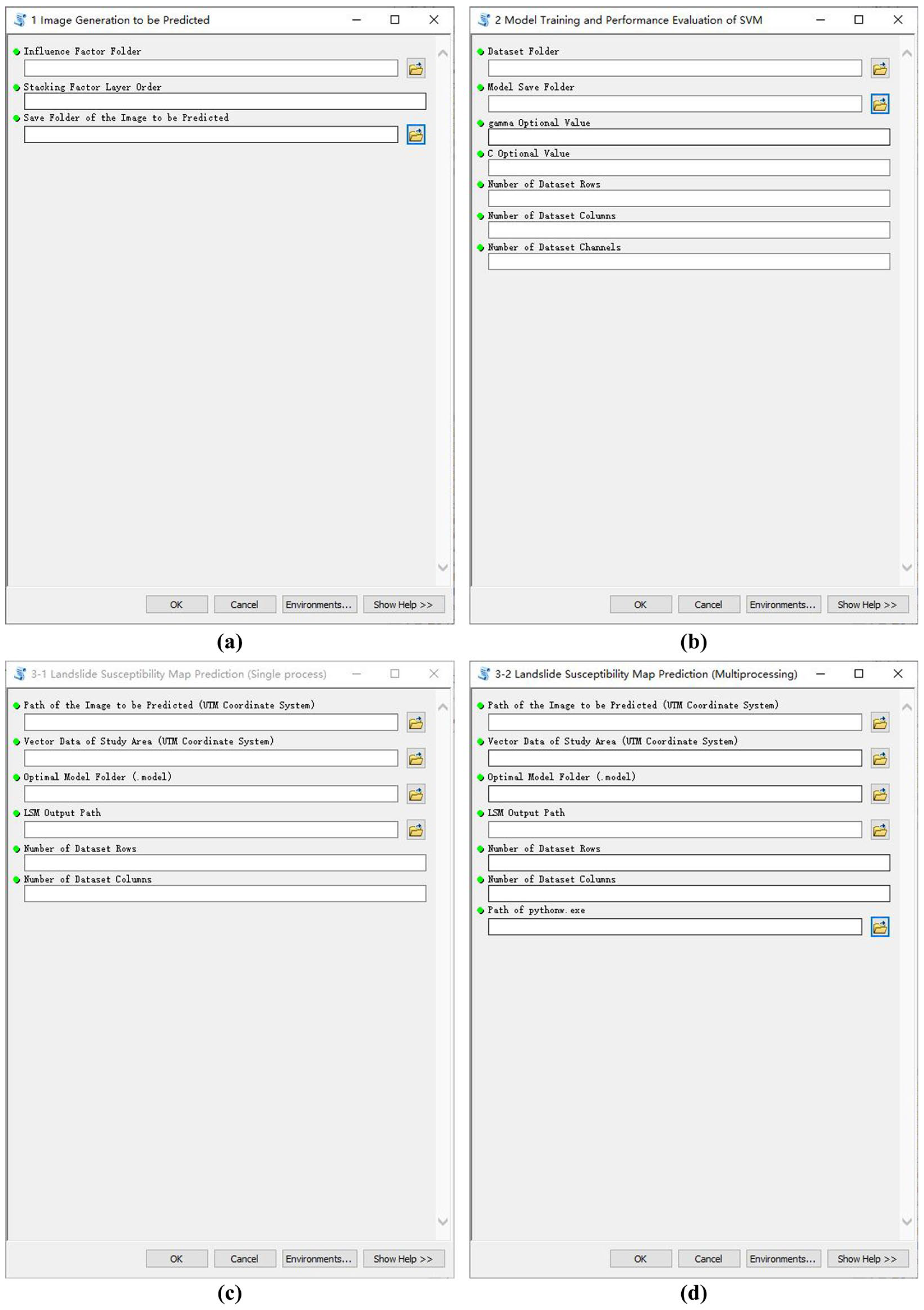
2.4. Model Training and Prediction
2.4.1. Image Generation to Be Predicted
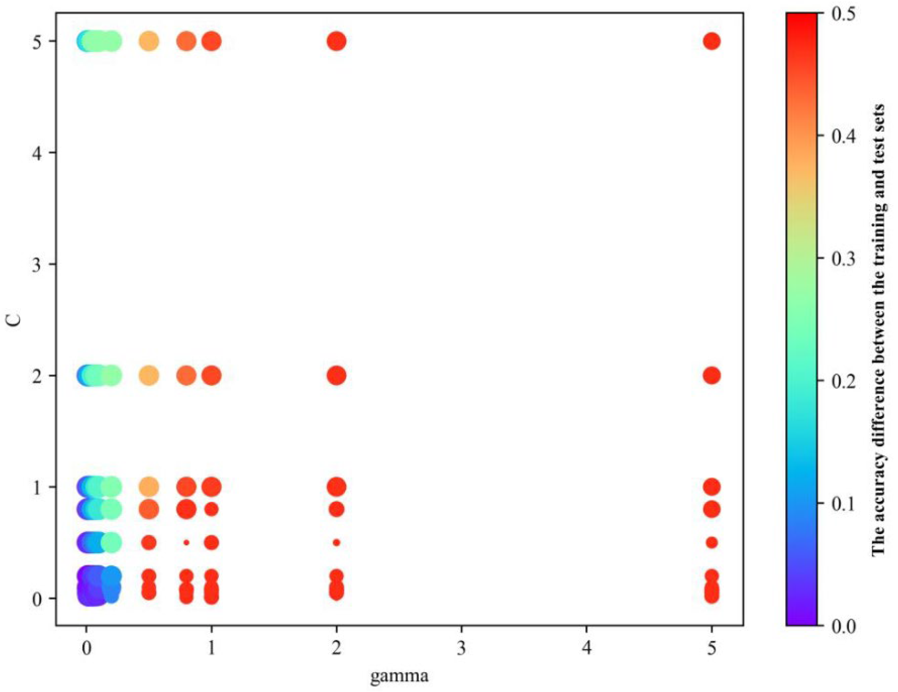
2.4.2. Model Training and Performance Evaluation of SVM
2.4.3. Landslide Susceptibility Map Prediction
3. Results
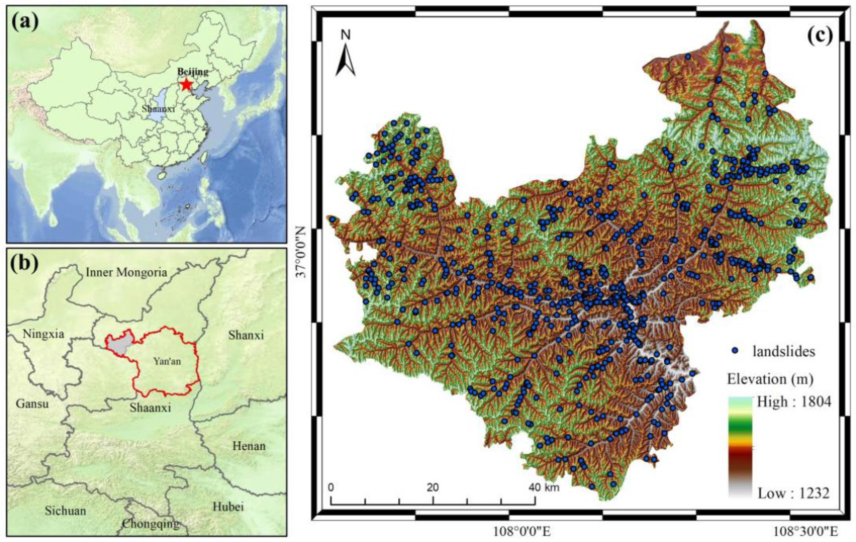
3.1. Study Area
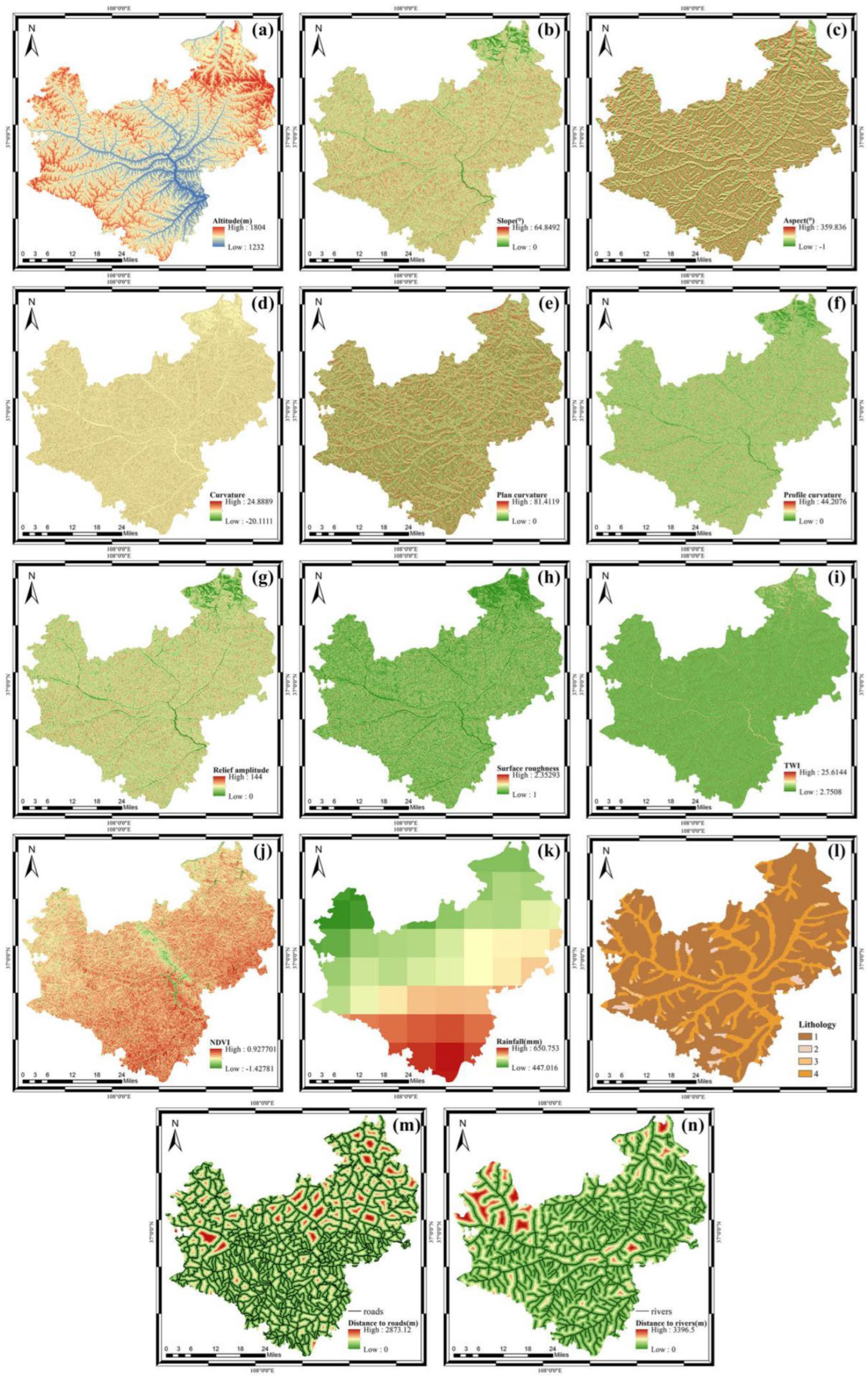
3.2. Preprocessing of Influencing Factors
3.3. Factor Selection and Sample Generation
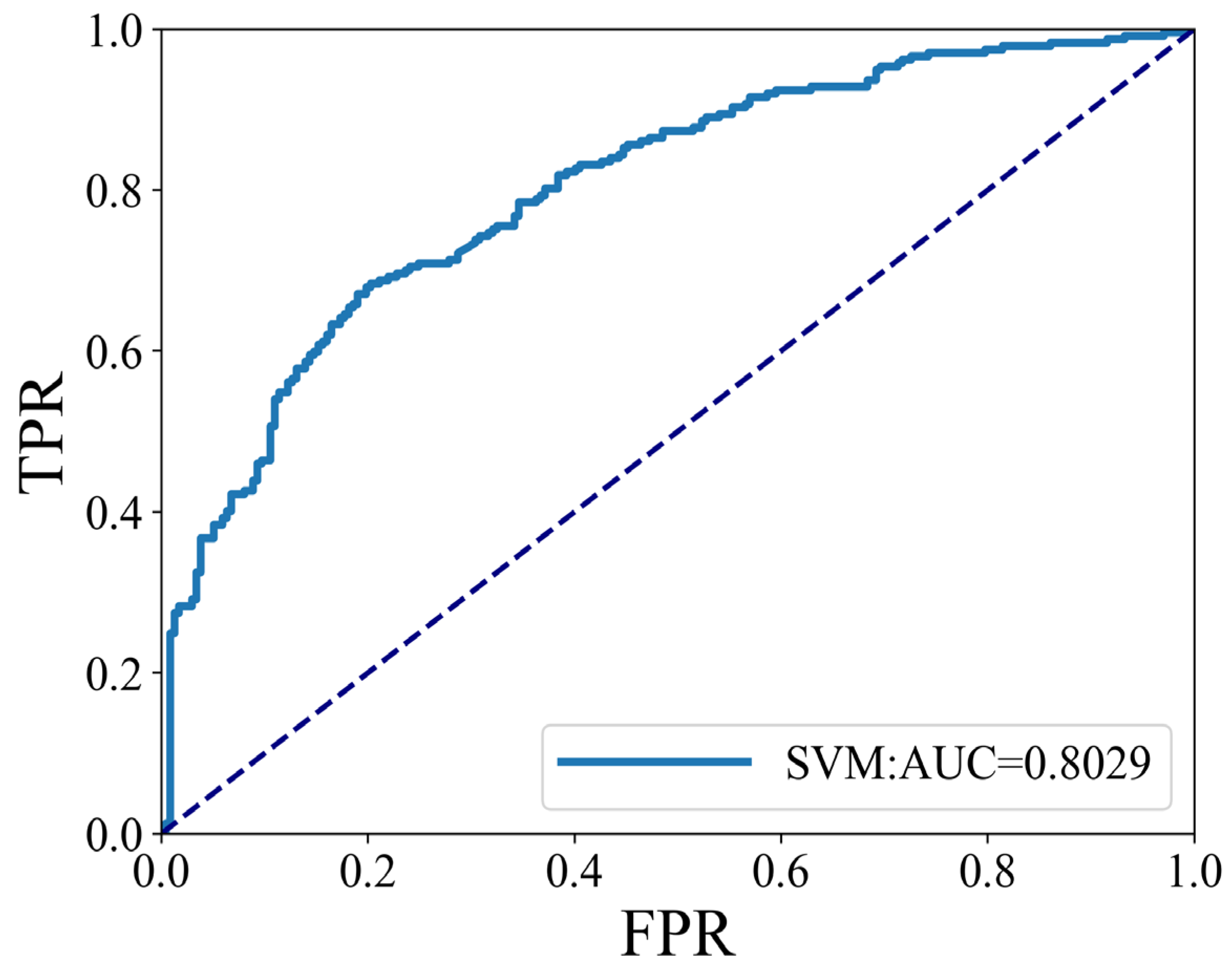
3.4. Model Training and Performance Evaluation
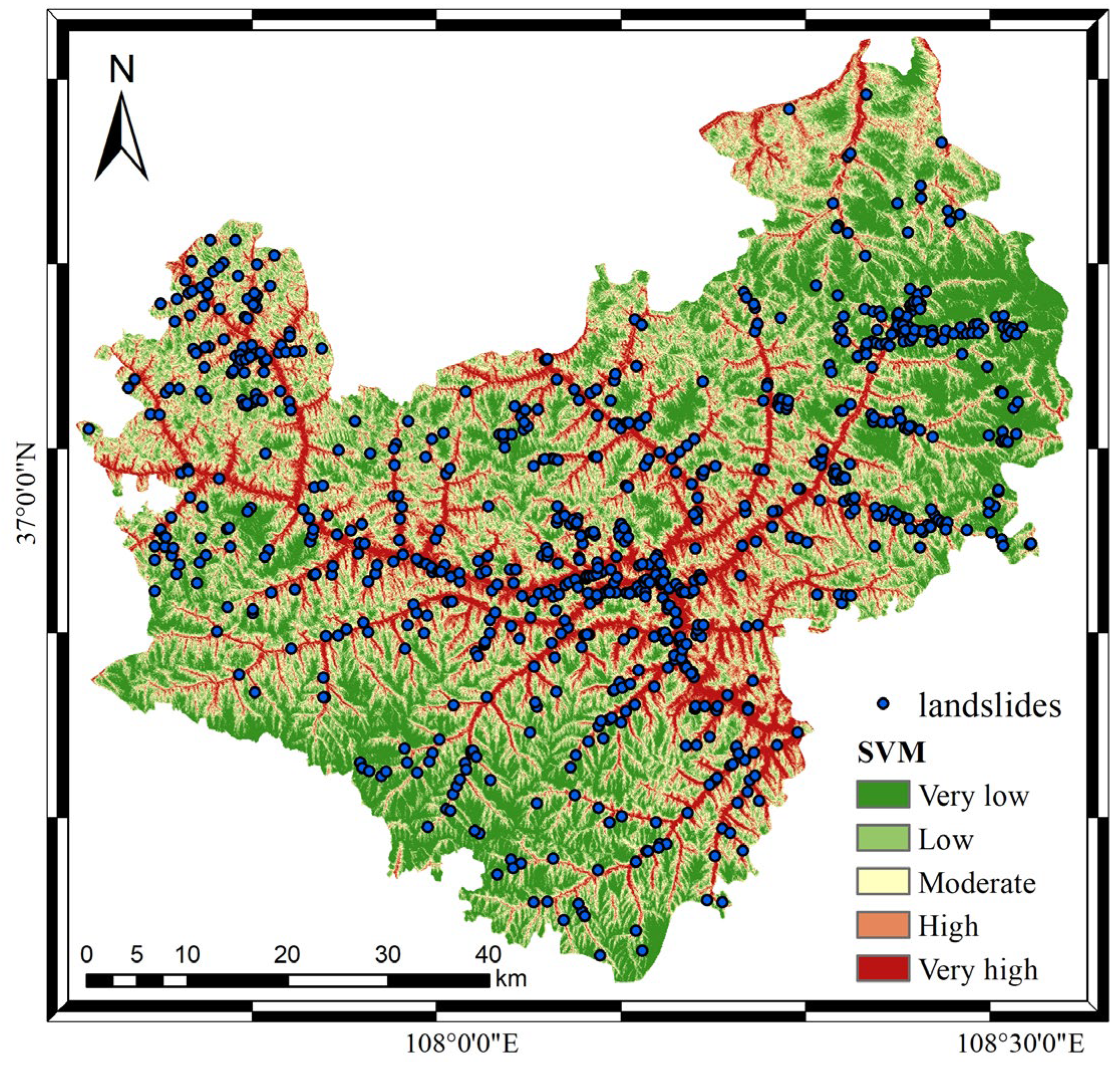
3.5. Landslide Susceptibility Map Generation and Analysis
3.6. Toolbox Operation Efficiency Evaluation
3.7. Model Selection: SVM
4. Conclusions
Author Contributions
Funding
Data Availability Statement
Conflicts of Interest
References
- Koley, B.; Nath, A.; Saraswati, S.; Chatterjee, U.; Bandyopadhyay, K.; Bhatta, B.; Ray, B.C. Assessment of spatial distribution of rain-induced and earthquake-triggered landslides using geospatial techniques along North Sikkim Road Corridor in Sikkim Himalayas, India. GeoJournal 2022, 1–39. [Google Scholar] [CrossRef]
- Zêzere, J.L.; Pereira, S.; Melo, R.; Oliveira, S.C.; Garcia, R.A.C. Mapping landslide susceptibility using data-driven methods. Sci. Total Environ. 2017, 589, 250–267. [Google Scholar] [CrossRef] [PubMed]
- Camera, C.A.S.; Bajni, G.; Corno, I.; Raffa, M.; Stevenazzi, S.; Apuani, T. Introducing intense rainfall and snowmelt variables to implement a process-related non-stationary shallow landslide susceptibility analysis. Sci. Total Environ. 2021, 786, 147360. [Google Scholar] [CrossRef] [PubMed]
- Qi, T.; Zhao, Y.; Meng, X.; Chen, G.; Dijkstra, T. AI-Based Susceptibility Analysis of Shallow Landslides Induced by Heavy Rainfall in Tianshui, China. Remote Sens. 2021, 13, 1819. [Google Scholar] [CrossRef]
- Xu, C.; Dai, F.; Xu, X.; Lee, Y.H. GIS-based support vector machine modeling of earthquake-triggered landslide susceptibility in the Jianjiang River watershed, China. Geomorphology 2012, 145-146, 70–80. [Google Scholar] [CrossRef]
- Yang, X.; Liu, R.; Yang, M.; Chen, J.; Liu, T.; Yang, Y.; Chen, W.; Wang, Y. Incorporating Landslide Spatial Information and Correlated Features among Conditioning Factors for Landslide Susceptibility Mapping. Remote Sens. 2021, 13, 2166–2190. [Google Scholar] [CrossRef]
- Costache, R.; Ali, S.A.; Parvin, F.; Pham, Q.B.; Arabameri, A.; Nguyen, H.; Crăciun, A.; Anh, D.T. Detection of areas prone to flood-induced landslides risk using certainty factor and its hybridization with FAHP, XGBoost and deep learning neural network. Geocarto Int. 2021, 1–36. [Google Scholar] [CrossRef]
- Ma, Z.; Mei, G.; Piccialli, F. Machine learning for landslides prevention: A survey. Neural Comput. Appl. 2020, 33, 10881–10907. [Google Scholar] [CrossRef]
- Reichenbach, P.; Rossi, M.; Malamud, B.D.; Mihir, M.; Guzzetti, F. A review of statistically-based landslide susceptibility models. Earth Sci. Rev. 2018, 180, 60–91. [Google Scholar] [CrossRef]
- Bathrellos, G.D.; Skilodimou, H.D.; Chousianitis, K.; Youssef, A.M.; Pradhan, B. Suitability estimation for urban development using multi-hazard assessment map. Sci. Total Environ. 2017, 575, 119–134. [Google Scholar] [CrossRef]
- Sezer, E.A.; Nefeslioglu, H.A.; Osna, T. An expert-based landslide susceptibility mapping (LSM) module developed for Netcad Architect Software. Comput. Geosci. 2017, 98, 26–37. [Google Scholar] [CrossRef]
- Medina, V.; Hürlimann, M.; Guo, Z.; Lloret, A.; Vaunat, J. Fast physically-based model for rainfall-induced landslide susceptibility assessment at regional scale. Catena 2021, 201, 105213. [Google Scholar] [CrossRef]
- Chowdhuri, I.; Pal, S.C.; Arabameri, A.; Ngo, P.T.T.; Chakrabortty, R.; Malik, S.; Das, B.; Roy, P. Ensemble approach to develop landslide susceptibility map in landslide dominated Sikkim Himalayan region, India. Environ. Earth Sci. 2020, 79, 476. [Google Scholar] [CrossRef]
- Li, L.; Lan, H.; Guo, C.; Zhang, Y.; Li, Q.; Wu, Y. A modified frequency ratio method for landslide susceptibility assessment. Landslides 2017, 14, 727–741. [Google Scholar] [CrossRef]
- Zhang, Y.-x.; Lan, H.-x.; Li, L.-p.; Wu, Y.-m.; Chen, J.-h.; Tian, N.-m. Optimizing the frequency ratio method for landslide susceptibility assessment: A case study of the Caiyuan Basin in the southeast mountainous area of China. J. Mt. Sci. 2020, 17, 340–357. [Google Scholar] [CrossRef]
- Goyes-Peñafiel, P.; Hernandez-Rojas, A. Landslide susceptibility index based on the integration of logistic regression and weights of evidence: A case study in Popayan, Colombia. Eng. Geol. 2021, 280, 105958. [Google Scholar] [CrossRef]
- Sun, D.; Xu, J.; Wen, H.; Wang, D. Assessment of landslide susceptibility mapping based on Bayesian hyperparameter optimization: A comparison between logistic regression and random forest. Eng. Geol. 2021, 281, 105972. [Google Scholar] [CrossRef]
- Wang, Y.; Feng, L.; Li, S.; Ren, F.; Du, Q. A hybrid model considering spatial heterogeneity for landslide susceptibility mapping in Zhejiang Province, China. Catena 2020, 188, 104425. [Google Scholar] [CrossRef]
- Fang, Z.; Wang, Y.; Duan, G.; Peng, L. Landslide Susceptibility Mapping Using Rotation Forest Ensemble Technique with Different Decision Trees in the Three Gorges Reservoir Area, China. Remote Sens. 2021, 13, 238. [Google Scholar] [CrossRef]
- Osna, T.; Sezer, E.A.; Akgun, A. GeoFIS: An integrated tool for the assessment of landslide susceptibility. Comput. Geosci. 2014, 66, 20–30. [Google Scholar] [CrossRef]
- Jebur, M.N.; Pradhan, B.; Shafri, H.Z.M.; Yusoff, Z.M.; Tehrany, M.S. An integrated user-friendly ArcMAP tool for bivariate statistical modelling in geoscience applications. Geosci. Model Dev. 2015, 8, 881–891. [Google Scholar] [CrossRef] [Green Version]
- Torizin, J.; Schüßler, N.; Fuchs, M. Landslide Susceptibility Assessment Tools v1.0.0b—Project Manager Suite: A new modular toolkit for landslide susceptibility assessment. Geosci. Model Dev. 2022, 15, 2791–2812. [Google Scholar] [CrossRef]
- Bragagnolo, L.; da Silva, R.V.; Grzybowski, J.M.V. Landslide susceptibility mapping with r.landslide: A free open-source GIS-integrated tool based on Artificial Neural Networks. Environ. Model. Softw. 2020, 123, 104565. [Google Scholar] [CrossRef]
- Sahin, E.K.; Colkesen, I.; Acmali, S.S.; Akgun, A.; Aydinoglu, A.C. Developing comprehensive geocomputation tools for landslide susceptibility mapping: LSM tool pack. Comput. Geosci. 2020, 144, 104592. [Google Scholar] [CrossRef]
- Guo, Z.; Torra, O.; Hürlimann, M.; Abancó, C.; Medina, V. FSLAM: A QGIS plugin for fast regional susceptibility assessment of rainfall-induced landslides. Environ. Model. Softw. 2022, 150, 105354. [Google Scholar] [CrossRef]
- Bartolini, S.; Cappello, A.; Marti, J.; Negro, C. QVAST: A new Quantum GIS plugin for estimating volcanic susceptibility. Nat. Hazards Earth Syst. Sci. Discuss. 2013, 1, 4223–4256. [Google Scholar] [CrossRef] [Green Version]
- Gaidzik, K.; Ramírez-Herrera, M.T. The importance of input data on landslide susceptibility mapping. Sci. Rep. 2021, 11, 19334. [Google Scholar] [CrossRef]
- Regmi, N.R.; Giardino, J.R.; McDonald, E.V.; Vitek, J.D. A comparison of logistic regression-based models of susceptibility to landslides in western Colorado, USA. Landslides 2013, 11, 247–262. [Google Scholar] [CrossRef]
- Pourghasemi, H.R.; Yansari, Z.T.; Panagos, P.; Pradhan, B. Analysis and evaluation of landslide susceptibility: A review on articles published during 2005–2016 (periods of 2005–2012 and 2013–2016). Arab. J. Geosci. 2018, 11, 193. [Google Scholar] [CrossRef]
- Stanley, T.A.; Kirschbaum, D.B.; Benz, G.; Emberson, R.A.; Amatya, P.M.; Medwedeff, W.; Clark, M.K. Data-Driven Landslide Nowcasting at the Global Scale. Front. Earth Sci. 2021, 9, 378. [Google Scholar] [CrossRef]
- Tien Bui, D.; Ho, T.-C.; Pradhan, B.; Pham, B.-T.; Nhu, V.-H.; Revhaug, I. GIS-based modeling of rainfall-induced landslides using data mining-based functional trees classifier with AdaBoost, Bagging, and MultiBoost ensemble frameworks. Environ. Earth Sci. 2016, 75, 1101–1123. [Google Scholar] [CrossRef]
- Awad, M.; Khanna, R. Support Vector Machines for Classification. In Efficient Learning Machines: Theories, Concepts, and Applications for Engineers and System Designers; Awad, M., Khanna, R., Eds.; Apress: Berkeley, CA, USA, 2015; pp. 39–66. [Google Scholar]
- Pradhan, B. A comparative study on the predictive ability of the decision tree, support vector machine and neuro-fuzzy models in landslide susceptibility mapping using GIS. Comput. Geosci. 2013, 51, 350–365. [Google Scholar] [CrossRef]
- Wang, S.; Zhuang, J.; Zheng, J.; Fan, H.; Kong, J.; Zhan, J. Application of Bayesian Hyperparameter Optimized Random Forest and XGBoost Model for Landslide Susceptibility Mapping. Front. Earth Sci. 2021, 9, 617. [Google Scholar] [CrossRef]


| Evaluation Index | Results | ||
|---|---|---|---|
| Confusion matrix | Landslide | Non-landslide | |
| Landslide | 169 | 68 | |
| Non-landslide | 66 | 171 | |
| Accuracy | 0.7173 | ||
| Precision | 0.7155 | ||
| Recall | 0.7215 | ||
| F1 | 0.7185 | ||
| AUC | 0.8029 | ||
| Classes | Area (km2) | Proportion (%) | Landslide Density (Number/km2) |
|---|---|---|---|
| Very low | 924.43 | 24.28 | 0.04 |
| Low | 948.24 | 24.90 | 0.08 |
| Moderate | 794.02 | 20.85 | 0.14 |
| High | 648.42 | 17.03 | 0.28 |
| Very high | 493.02 | 12.94 | 0.77 |
| Tool | ArcGIS | ArcGIS Pro | |
|---|---|---|---|
| Topographic factor calculation | 58 s | 42 s | |
| Convert line vector data to continuous raster factor | 1 min 9 s | 34 s | |
| Rainfall data processing | 57 s | 50 s | |
| Batch clipping of each factor layer | 18 s | 17 s | |
| Non-landslide data generation | 2 s | 1 s | |
| Data sample production * | landslide | 5 min 22 s/4 min 46 s | 4 min 34 s/4 min 29 s |
| non-landslide | 4 min 56 s/4 min 32 s | 4 min 19 s/4 min 15 s | |
| Dataset split * | 0.5 s/0.5 s | 0.5 s/0.5 s | |
| PCC and IGR calculation | 1 min 16 s | 57 s | |
| Image generation to be predicted * | 3 min 38 s/2 min 45 s | 1 min 32 s/1 min 13 s | |
| Model training and performance evaluation of SVM | 1 h 55 min 32 s | 1 h 8 min 8 s | |
| Landslide susceptibility map prediction (single process) | 2 h 53 min 15 s | 1 h 26 min 47 s | |
| Landslide susceptibility map prediction (multiprocessing) | 21 min 51 s | 20 min 12 s | |
| Total † | 5 h 19 min 27 s/2 h 48 min 3 s | 2 h 58 min 39 s/1 h 52 min 4 s | |
| Model | Number of Parameters | Training Time Complexity | LSM Prediction (Multiprocessing) | AUC |
|---|---|---|---|---|
| DT | 2 | 4 min 28 s | 0.7774 | |
| RF | 5 | 1 h 21 min 25 s | 0.8372 | |
| SVM (this study) | 2 | 20 min 12 s | 0.8029 |
Publisher’s Note: MDPI stays neutral with regard to jurisdictional claims in published maps and institutional affiliations. |
© 2022 by the authors. Licensee MDPI, Basel, Switzerland. This article is an open access article distributed under the terms and conditions of the Creative Commons Attribution (CC BY) license (https://creativecommons.org/licenses/by/4.0/).
Share and Cite
Huang, W.; Ding, M.; Li, Z.; Zhuang, J.; Yang, J.; Li, X.; Meng, L.; Zhang, H.; Dong, Y. An Efficient User-Friendly Integration Tool for Landslide Susceptibility Mapping Based on Support Vector Machines: SVM-LSM Toolbox. Remote Sens. 2022, 14, 3408. https://doi.org/10.3390/rs14143408
Huang W, Ding M, Li Z, Zhuang J, Yang J, Li X, Meng L, Zhang H, Dong Y. An Efficient User-Friendly Integration Tool for Landslide Susceptibility Mapping Based on Support Vector Machines: SVM-LSM Toolbox. Remote Sensing. 2022; 14(14):3408. https://doi.org/10.3390/rs14143408
Chicago/Turabian StyleHuang, Wubiao, Mingtao Ding, Zhenhong Li, Jianqi Zhuang, Jing Yang, Xinlong Li, Ling’en Meng, Hongyu Zhang, and Yue Dong. 2022. "An Efficient User-Friendly Integration Tool for Landslide Susceptibility Mapping Based on Support Vector Machines: SVM-LSM Toolbox" Remote Sensing 14, no. 14: 3408. https://doi.org/10.3390/rs14143408