1. Introduction
With the development of sensors, the coverage provided by remote sensing images has widened and the spatial resolution has become finer. Due to their capability to describe ground information in detail, remote sensing images have been widely used in land resource monitoring and urban resource management [
1,
2,
3]. Semantic segmentation of a scene is the key issue during remote sensing image processing, which divides the whole space into multiple regions of interest by clustering each pixel [
4,
5]. Recently, the spatial resolution of remote sensing images has reached the centimeter level, and such advances in technology produce more redundant image information and noise, so semantic segmentation tasks are becoming increasingly challenging [
6].
Traditional methods of semantically segmenting remote sensing images, such as the maximum likelihood [
7], minimum distance [
8], and iterative self-organizing data analysis techniques algorithm (ISODATA) [
9], have been widely used for classifying land use and land cover. Considering only the digital number value of each pixel during classification process, most traditional methods separate the connection between the current pixel and surrounding ones. To some extent, their limitations are low classification accuracy and poor adaptability to complex samples.
Deep learning has enabled considerable breakthroughs in many fields and shown remarkable performance in image processing. With its strong ability to express features and fit data, many different types of deep learning models are widely used in semantic segmented tasks [
10,
11,
12]. Compared with traditional classification methods, deep learning models consider the spatial relationship between adjacent pixels, so can achieve high-quality performance when dealing with complex geographic object samples [
13]. For semantic segmentation tasks, deep learning methods generally use convolutional neural networks (CNNs) to capture image features and provide an initial class label for each pixel in the image. On this basis, a series of improved deep learning models has also been constructed [
14]. For instance, to accept input images of any size, fully convolutional networks (FCNs) use a convolutional layer instead of a fully connected layer [
15]. However, due to the existence of the pooling layer, multiple convolutions and pooling operations continually expand the receptive field and aggregate information. The downsampling process continuously reduces the spatial resolution of the image, thus eventually resulting in the loss of global context information. U-net, used for medical image segmentation proposed by Ronnerberge, combines different feature maps within the channel dimension to form denser features [
16]. However, U-net reduces the convergence speed of the network for a larger number of sample categories. Then, when training large data sets, the amount of calculation increases, resulting in higher training costs. Due to the complex ground information contained in remote sensing images, many objects have similar appearances, so can be easily confused when performing semantic segmentation tasks. The pyramid scene parsing network (PSPNet) proposed by Zhao adopts the spatial pyramid pooling (SPP) module through which local and global information are added to the feature map [
17]. The PSPNet enables the model to consider more global context information and promote the fusion of multiscale features. The result is that the model effectively improves the accuracy of semantic segmentation. Similar to PSPNet, DeeplabV3plus, proposed by Chen, also considers more context information and has higher segmentation accuracy [
18]. However, the main difference is that it adopts the atrous-spatial pyramid pooling (ASPP) module. DeeplabV3plus uses a simple, effective encoder–decoder structure to increase the detection speed of the network, and it expands the receptive field and captures large amounts of local information to achieve an accurate segmentation effect.
In remote sensing images, many different types of ground objects are mixed, which creates challenges in semantic segmentation tasks. Therefore, to achieve the semantic segmentation of remote sensing images, deep learning networks need to be improved to capture important edge and texture features. Based on the native FCN, Mou et al. [
19] proposed a recurrent network in a fully convolutional network (RiFCN), using a forward stream to generate multilevel feature maps and a backward stream to generate a fused feature map as the classification basis. Although RiFCN performs well in semantic segmentation, the constant replacement of its network parameters results in large computational costs. Du et al. integrated the object-based image analysis method (OBIA) with the DeeplabV3plus model [
20]. This design effectively optimizes the segmentation results, but the increase in parameters complicates the network structure, which increases the training cost.
Recently, the domain of embedding attention mechanisms into neural networks has considerably advanced [
21,
22]. The attention mechanism is the behavior of selectively processing signals. This is an optimization strategy for many organisms, including humans, when processing external signals, and the mechanism behind it is called the attention mechanism by scholars in the field of cognitive science. For example, Jun et al. designed DANet, which introduces the dual attention (DA) module into the semantic segmentation task [
23]. DANet uses the position attention and the channel attention modules to enhance the expression of image features. From the perspective of the segmentation effect, the DA module has an accurate localization ability without increasing the computational cost too much. The convolutional block attention module (CBAM), proposed by Woo et al. [
24], similar to DA, also includes a spatial attention module and a channel attention module. Unlike the parallel structure of the DA module, CBAM is more lightweight and has a series structure, which considerably reduces the computational burden when training the network. Therefore, the network performance can be effectively improved by integrating the attention module into the semantic segmentation network of remote sensing images [
25]. Guo et al. designed the multitask parallel attention convolutional network (MTPA-Net) for the semantic segmentation of high-resolution remote sensing images via integrating the CBAM and DA into a CNN, which effectively reduced the misclassified areas and improved the classification accuracy [
26]. Li designed a semantic segmentation network with spatial and channel attention (SCAttNet) by embodying the CBAM into a CNN, which also achieved accurate segmentation in the semantic segmentation task for remote sensing images [
27].
However, it is not enough only to use the attention module for network improvement. In DeeplabV3plus, the ASPP only uses convolution blocks with atrous convolution rates of 6, 8, and 12, respectively, thereby limiting the richness of information scales and ignoring the recognition and detection of small objects. Yang et al. designed DenseASPP [
28], which takes full advantage of the parallel and cascaded architecture of dilated convolutional layers to obtain semantic information at more scales. However, the dense connection method will have particularly thick features, and there may be more repetitions. The too deep network is prone to cause overfitting and gradient disappearance. To solve the above problems, we design a new type of ASPP and name residual ASPP, which reconstructs ASPP with the dilated attention convolution unit and contains five dilated attention convolution modules with atrous convolution rates of 3, 6, 12, 18, and 24 to obtain important semantic information at more scales. The residual unit reduces the complexity of the model and prevents the gradient from vanishing.
Our main aims and highlights in this study are as follows:
- (1)
We designed a novel Residual ASPP structure, which reconstructs the atrous convolution unit with the dilated attention convolution unit, obtains important semantic information at multiple scales, and reduces the complexity of the network through the residual unit.
- (2)
In residual ASPP, we used different attention modules to design comparative experiments and ablation experiments of CBAM and DA, and specifically compared the similarities and differences between the two attention modules.
- (3)
To verify the accuracy improvements produced by the proposed methods with those of the native DeeplabV3plus model and other deep learning models. The proposed model achieves state-of-the-art performance on the LoveDA dataset and the ISPRS Vaihingen dataset.
The remainder of this paper is arranged as follows: the materials and methods are introduced in
Section 2; the experimental results are illustrated in
Section 3, and the discussions and conclusions are presented in
Section 4 and
Section 5, respectively.
2. Materials and Methods
2.1. Data Sources
We selected the land-cover domain adaptive semantic segmentation (LoveDA) dataset [
29] as the research object, which includes 5987 remote sensing images with 3 m (high) spatial resolution, and each image has a resolution of 1024 × 1024 in the dataset. The dataset comprises remote sensing images derived from different urban and rural areas of Nanjing, Changzhou, and Wuhan, China. It contains 6 land-use categories, including building, road, water, barren, forest, and agriculture. Due to the complex background, multiscale objects, and inconsistent class distributions, the dataset presents challenges for semantic segmentation tasks.
2.2. Related Methods
In this section, we introduce the principle of the DeeplabV3plus model, CBAM, and DA module, and illustrate the structure of DEAM in detail.
2.2.1. Atrous-Spatial Pyramid Pooling
ASPP is an improvement framework of SPP. The prominent difference from SPP is that ASPP uses an atrous convolution in place of the ordinary convolution. Through this improvement, ASPP can obtain a larger receptive field and enrich the obtained semantic information. Compared with SPP, ASPP can obtain a larger receptive field and enrich the obtained semantic information. The specific process of ASPP is as follows. Given a feature, a 1 × 1 convolutional layer, a 3 × 3 convolutional layer with expansion rates of 6, 12, and 18, and an average pooling layer were input, respectively. Next, the output results were merged as a multi-scale fusion feature map, which considered the output feature map of ASPP.
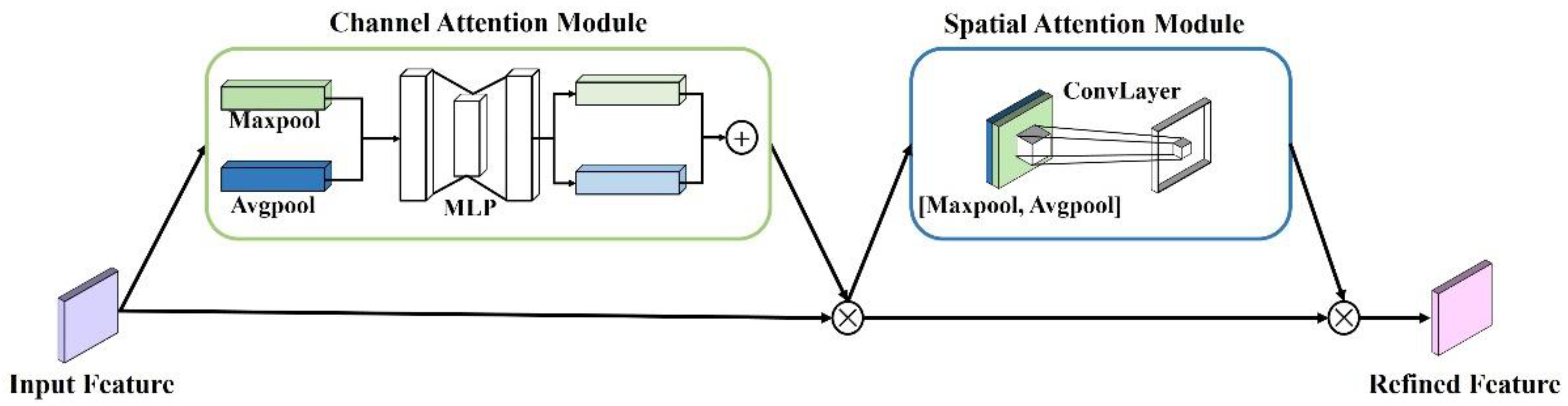
2.2.2. Convolutional Block Attention Module
CBAM is a lightweight attention module for feed-forward convolutional neural networks, and it can be seamlessly integrated into any CNN architecture (
Figure 1). It separately and sequentially infers the attention maps through the channel and spatial dimensions. The specific process is as follows: First, input feature map
into the channel attention module to obtain the intermediate feature map and multiply the intermediate feature map by the feature map
F to obtain the feature map
. Then, input the feature map
into the spatial attention module; the output intermediate feature map is multiplied by the feature map
to obtain the final feature map
. The main process is as follows:
In the channel attention module, the input feature
is input to the maximum pooling (Maxpool) and the average pooling (Avgpool) layer, respectively, to generate two different features. Both features were then forwarded to the multilayer perceptron (MLP) to produce the channel attention map
. The formula is as follows:
where,
represents the channel attention map,
represents the sigmoid function.
The channel attention module compresses the spatial dimension of the input feature map, uses the Avgpool and Maxpool operations to aggregate the channel information from the feature map, and generates two different pieces of spatial contextual information. After their matrix addition, the result is multiplied by the input feature. These operations improve the effectiveness of the information of the important features and enhance the expressiveness of features.
In the spatial attention module, two feature maps are generated by aggregating the channel information of a feature map by using Avgpool and Maxpool operations and are then concatenated and convolved by a standard convolution layer (including convolution, normalization, and ReLU activation function) to produce the spatial attention map
. The processing is as follows:
where
represents the spatial attention map,
represents a convolutional layer with a 7 × 7 kernel.
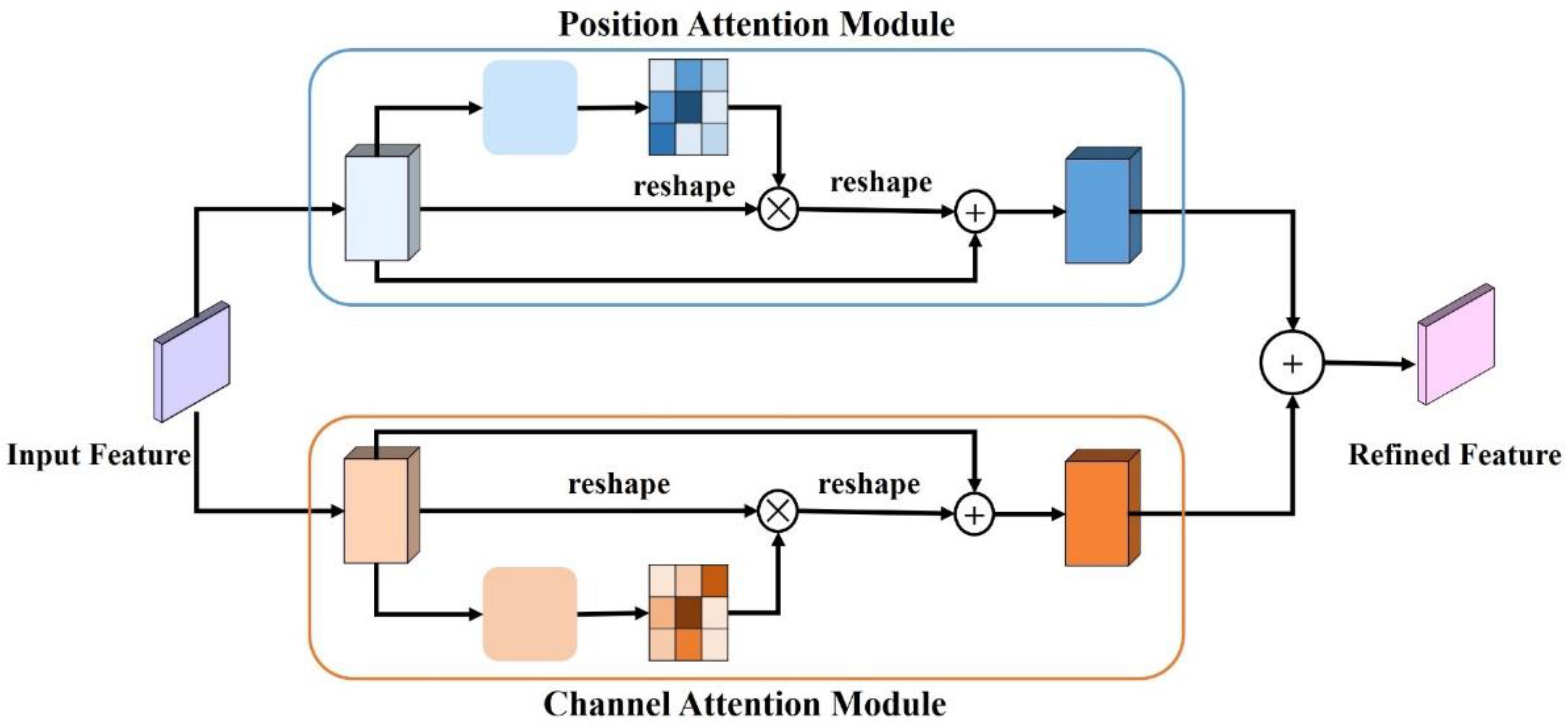
2.2.3. Dual Attention Module
The DA module also has a position attention module and a channel attention module, but it adopts a parallel instead of a series architecture (
Figure 2). The process involves inputting the feature maps into the position attention module and the channel attention module separately, then their output feature maps are added element by element to obtain the output feature map of the DA module.
In the position attention module, first, we fed local feature A into a convolution layer to generate three new feature maps: B, C, and D. Then, we reshaped them to C × N (N = H × W). After, we performed a matrix multiplication between the transpose of C and B, and applied a SoftMax layer to calculate the spatial attention map S. Then, we performed a matrix multiplication between D and the transpose of S and reshaped the result to C × H × W. Finally, we multiplied it by a scale parameter α and performed an element-wise sum operation with the features A to obtain the final output feature map E.
The process can be represented by the following formula:
where
is the
ith position’s impact on the
jth position,
represents the
ith position of feature map B,
represents the
jth position of feature map C,
represents the
jth position of feature map E,
represents the
ith position of feature map D,
represents the
jth position of feature map A, and
α is initialized as 0 and gradually learns to assign more weight.
Because the output feature map E at each position is a weighted sum of the features across all positions and original features, feature map E has a global contextual view and selectively aggregates contexts according to the spatial attention map, thus enhancing the expressiveness of the spatial information. The principle of the channel attention module is similar to that of the position attention module. The only difference is that the input feature map A is not used to generate features B, C, and D, but is directly used to calculate the channel attention map X, and the scale parameter
β is used to calculate the final output feature E. The process can be represented as:
where
represents the
ith channel’s impact on
jth channel,
represents the
jth position of feature map A, and
gradually learns a weight from 0.
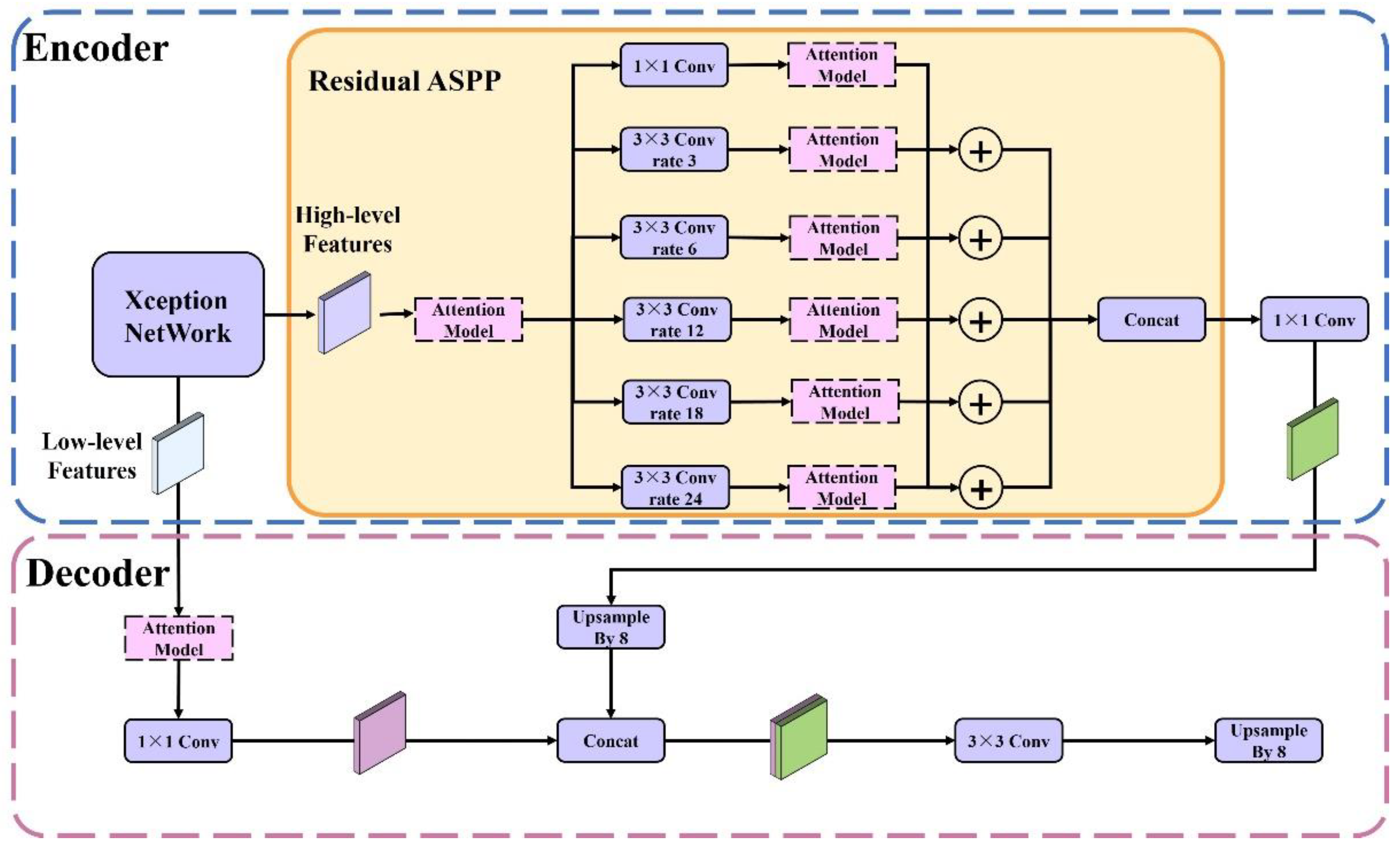
2.3. Framework of the RAANet
The proposed framework of RAA-Net is shown in
Figure 3. It consists of two parts: encoder and decoder.
In the encoder, a low-level feature and a high-level feature are output. The low-level feature is extracted by the Xception backbone network, and it mainly contains shallow information such as the outline and shape features. The high-level feature is processed by the backbone network and the residual ASPP, and it mainly contains deep information such as the texture and color features.
In residual ASPP, the original features are input into 5 dilated attention convolution units and a residual unit, respectively. Each dilated attention convolution unit was composed of an atrous convolution module and an attention module, while the residual unit was composed of 1 × 1 convolution modules and attention modules. Among them, the dilated convolution rates of the five dilated convolutional attention are 3, 6, 12, 18, and 24, respectively, and the size of the convolution kernel is 3 × 3. Then, the output of each dilated attention convolution unit is matrix added with the output of the residual unit respectively to obtain five output feature maps of the residual ASPP. Finally, the five feature maps are merged with the concatenation operation and the merged result is then input into the 1 × 1 convolution module. The high-level features are obtained eventually through the above operations.
In the decoder, the low-level and high-level features output by the encoder are received. First, the low-level features are input into the attention module and the 1 × 1 convolutional layer to obtain a refined low-level feature map. Second, a fused feature map is obtained by using the concatenation operation to merge the high-level features after upsampling processing and the shallow features. Finally, the fused feature map is input into the 3 × 3 convolutional layer, and the upsampling process is performed to obtain the prediction basis of the network.
In the model, we use the improved Xception convolutional network as the feature extraction network, and the atrous convolution rates of the ASPP are 6, 12, and 18. We use DiceLoss [
30] and cross-entropy loss (CELoss) [
31] as the combined loss function. The related loss function formulas are as follows:
where
N represents the total number of samples;
represents the target value;
represents the predicted value;
I represents sum of target value times predicted value;
U represents sum of target value plus predicted value;
represents the smoothing coefficient, which takes a value of 1 × 10
−5 in this paper;
indicates the number of categories;
is the predicted probability distribution, and
is the real probability distribution.
3. Experimental Results
The LoveDA dataset was selected to provide the sample data for the segmentation task. All selected images were divided into training, validation, and test datasets, with 2365, 591, and 682 images, respectively. These images were inputted into DeeplabV3plus, DADP, and CBAMDP for training, and then the effects of three semantic segmentation methods were compared.
3.1. Evaluation Criteria
We used the mean intersection-over-union (mIoU), mRecall, mPrecision, and F1 scores to evaluate the overall impact of different attention models on the DeeplabV3plus network. Detailed explanations of TP, FP and FN are listed in
Table 1The IoU is the ratio of the intersection and union of the predicted result and ground truth in the segmentation of land-use types. The mIoU is a standard evaluation, which is the average IoU of all land-use types. The following formulas are used to calculate the two metrics:
The Recall is used to evaluate the ability of a classifier to find all positive samples, whereas mRecall is the average recall of all types, which are calculated as follows:
The Precision indicates the ability of a classifier to label a sample as positive that is positive, whereas mPrecision is the average precision of all types, which are calculated as follows:
The F1 score is defined as the harmonic mean of recall and precision; it pays attention to the precision and recall and provides an overall measurement of the performance of a change detection model. A higher F1 score represents more accurate performance, which is calculated as follows:
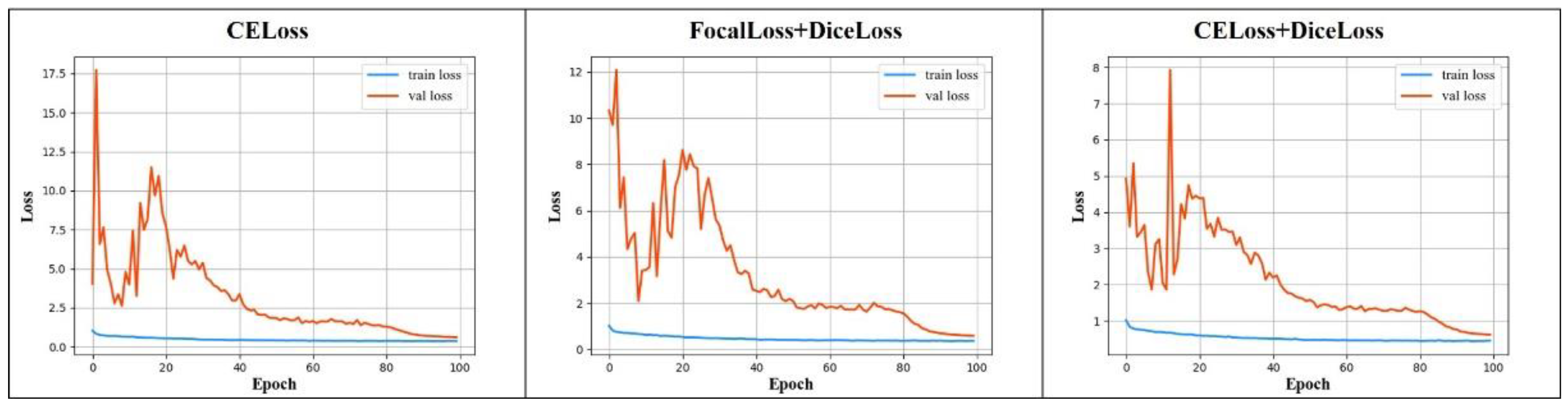
3.2. Determination of Loss Function
The decision of a suitable loss function is an important premise for deep learning model selection. The loss function describes the degree of disparity between the predicted result and the ground truth, and the value of the loss function directly reflects the performance of the model. Using different loss functions for the same model will bring different effects. Therefore, to ensure that the model achieves the best effect, it is necessary to select an appropriate loss function. CELoss is the most popular loss function used for multiclass classification, which is suitable for situations where each type in the dataset is independent but not mutually exclusive. DiceLoss is usually used for the loss evaluation of datasets with similar samples. Focal loss [
32] is a more suitable choice for dealing with difficult datasets with imbalanced data distribution. Thus, in this study, we focused on three loss functions, CELoss, CELoss + DiceLoss [
33], and FocalLoss + DiceLoss, to determine which was most suitable for the dataset we selected.
Figure 4 shows the loss value curves of the three kinds of loss functions. The ranges of loss values are different in the three functions. The maximum value of CELoss is around 17.5, CELoss + DiceLoss is around 12, and CELoss + DiceLoss is around 8. When CELoss is in the 24th generation, the loss value shows a steady downward trend, and it begins to converge in the 90th generation. FocalLoss + DiceLoss shows a slow decline trend in the 26th generation and begins to converge in the 90th generation, and CELoss + DiceLoss appears as a slow downward trend in the 23rd generation and converges in the 90th generation. In terms of the changing trend of the loss value, the loss function combination of CELoss + DiceLoss makes the loss value control in a smaller range, and it is easier to converge.
Next, we compared the evaluation indicators of the three loss functions. As shown in
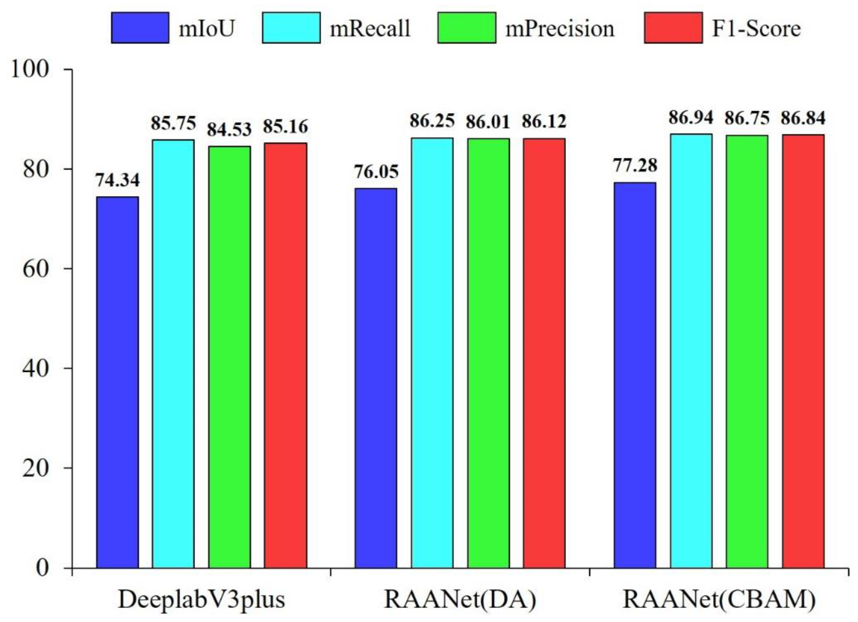
Table 2, when we used DiceLoss + CELoss, the model had the highest accuracy; the mIoU, mRecall, mPrecision, and F1score were 74.34%, 85.75%, 84.53%, and 85.16%, respectively, which were 1.01%, 2.07%, 0.56%, and 1.34% higher than those of the original CELoss, respectively, and which were 1.66%, 2.99%, 0.97%, and 2% higher than those of the FocalLoss + DiceLoss, respectively. The findings illustrated that the addition of DiceLoss was beneficial to solving the problem produced by similar samples in the dataset, and positively impacted model performance. Therefore, we used CELoss + DiceLoss for model training.
3.3. Results of Ablation Experiment
To verify the overall structure effectiveness of the proposed module, ablation experiments are conducted in this paper. The baseline structure is selected as the ASPP with expansion rates of 3, 6, 12, 18, and 24. Based on it, DA, CBAM, and residual structure are added, and the improvement effect of each module on ASPP is analyzed in detail.
Table 3 shows the results of the ablation experiments, according to each indicator, and the improvement of ASPP by DA and CBAM was 0.98%, 0.75%, 1.13%, 0.95%, and 1.4%, 1.06%, 1.09%, 1.08%, respectively. It shows that adding the attention module to 5 ASPP units can get a lot of improvement, and the improvement effect of CBAM is better than that of DA. When the residual structure is added, the improvement of ASPP + DA and ASPP + CBAM is different. Compared with ASPP + DA, the structure of ASPP + DA + Res is improved by 0.63%, 0.34%, 0.22%, 0.28%, respectively, and compared with the ASPP + CBAM, the structure of ASPP + CBAM + Res is improved by 1.04%, 0.4%, 1%, and 0.7%, respectively. When the ASPP structure is more complex, CBAM has a greater advantage.
The results of ablation experiments show that the residual structure and attention module have a significant improvement in ASPP. When the attention module and ASPP are simply connected, the improvement effect of CBAM and DA is not much different, but when the complexity of ASPP increases, CBAM has a greater advantage.
3.4. Visualization of Features
There are three types of feature maps displayed in
Figure 5. The first type is the low-level feature maps of the DeeplabV3plus, RAANet (DA), and RAANet (CBAM), respectively. Compared with DeeplabV3plus, the feature maps of the latter two contain richer boundary information, which results in a clearer outline of each land-use category.
The second type is the feature maps of five convolutional blocks in ASPP. In each feature map, the hotspot areas displayed by DeeplabV3plus are relatively balanced and cover almost all areas in the image. The hotspot areas displayed by RAANet (DA) are mainly concentrated in the bottom left barren and a few buildings, while that of RAANet (CBAM) are mainly concentrated on a single building and the bottom barren in the image.
The third type is the total output feature maps of ASPP. It can be found that the hot spots of RAANet (CBAM) clearly show the results of the classification of land-use categories, while RAANet (DA) are mainly concentrated in barren and buildings. The hotspot area of DeeplabV3plus is relatively sparse and mainly concentrated in the buildings. In the final prediction results, RAANet (DA) is more accurate for the prediction of the lower-left barren, RAANet (CBAM) achieves a better prediction effect for the building and road prediction, and DeeplabV3plus has a poor prediction effect on this image. Overall, RAANet (CBAM) contains richer semantic information, followed by RAANet (DA) and DeeplabV3plus last.
3.5. Comparison of Model Performance
We evaluated the overall performance of the three models using mIoU, mRecall, mPrecision, and F1 score to determine whether the integration of the attention module enhanced the expressiveness of the spatial and channel information from the images. As shown in
Figure 6, the mIoU, mRecall, mPrecision, and F1 score of RAANet (DA) were improved by 1.71%, 1.5%, 1.48%, and 0.96%. RAANet (CBAM) was more accurate, with mIoU, mRecall, mPrecision, and F1 score improved by 2.94%, 1.19%, 2.22%, and 1.68%, respectively.
To further compare the performance of the three models, we selected the mIoU, mRecall, and mPrecision indices to measure the segmentation results for different land-use categories.
Table 4 shows the IoU values for each category of the three models. Although the DA module had a positive impact on mIoU, its impacts on the IoU values of water were negative, with values reduced by 7%. The impacts of other categories were the opposite, and the IoU values increased by 3%, 4%, 4%, 3%, and 5%, respectively. RAANet (DA) raised the prediction accuracy of the background, building, road, barren, forest, and agriculture categories, but showed reduced prediction accuracy for the water category. The RAANet (CBAM) improved the IoU values of each category prediction by 4%, 4%, 2%, 1%, 3%, 3%, and 4%, respectively. RAANet (CBAM) obtained higher accuracy in predicting each category.
Table 5 shows the recall values for each category of the three models. Compared with the DeeplabV3plus, RAANet (DA) has obvious shortcomings in water, which reduces the recall value of water by 8%, but increased the prediction of other categories by 3%, 1%, 3%, 3%, and 3% respectively. In terms of RAANet (CBAM), it increased the detection accuracy of the background, building, road, and agriculture categories by 4%, 3%, 2%, and 3%, respectively.
The results showed that RAANet (DA) reduced the number of the correctly predicted pixels in the water category but increased in the other categories. RAANet (CBAM) correctly predicted more pixels in the background, building, road, and agriculture categories. The RAANet (DA) performed better in the road, barren, and forest categories than the other two models, but was lowest in the water category. The RAANet (CBAM) was best in the background and building categories.
Table 6 showed the precision values for each category of the three models. Compared with native DeeplabV3plus, RAANet (DA) had higher precision for building, barren, forest, and agriculture, which were increased by 3%, 2%, 3%, and 3%, respectively. The RAANet (CBAM) increased the recognition accuracies by 4%, 6%, 6%, and 6% for the background, building, road, barren, forest, and agriculture categories, respectively. However, the RAANet (CBAM) reduced precision by 2% for the road and water categories.
The results show that RAANet (DA) and RAANet (CBAM) increase the number of real positive pixels that are correctly predicted positive in building, barren, forest, and agriculture categories, but RAANet (CBAM) reduces the number of real positive pixels that are predicted positive in road and water categories. RAANet (DA) has a bigger advantage in precision.
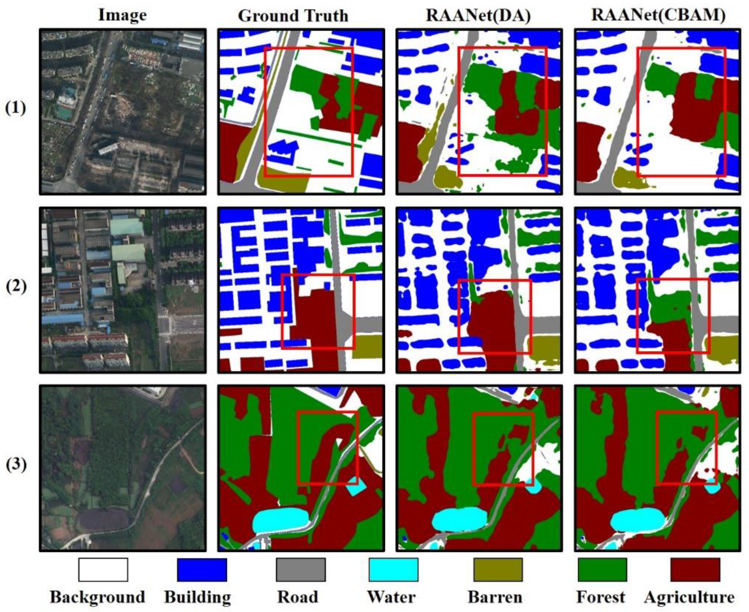
We compared the results predicted by the models with attention with those of the original model to verify whether the segmentation accuracy was improved. The real geographic object labels, the predicted results of the RAANet (DA) and RAANet (CBAM), and the prediction results of the original model are shown in
Figure 7.
There are errors in the Ground Truth, such as the fifth image in which there is forest and agriculture, but this is not embodied in Ground Truth. Consequently, Ground Truth cannot be directly used as the evaluation criterion. Both Ground Truth and images were considered in this analysis. Incorrect judgments in the predicted results for remote images were produced by the native DeeplabV3plus. Water, agriculture background, and barren were often confused. This appearance was shown in
Figure 7(1b,2b,4b).
The identify accuracy of RAANet (DA) on the water was great better than the native DeeplabV3plus, which can be shown in
Figure 7(1b,2b,5b). However, RAANet (DA) increased the number of pixels where the background was incorrectly judged as barren, as shown in
Figure 7(5c). In addition, the ability to distinguish between agriculture and forest was weak, as shown in
Figure 7(4c). The identification accuracy of CBAM on images was best. In short, RAANet has better performance in the loveDA dataset than Deeplabv3plus, and the prediction effect is more accurate. The overall performance of RAANet (CBAM) is higher than that of RAANet (DA), but RAANet (DA) performs better in Precision.
4. Discussion
To assess the performance of the improved DeeplabV3plus model embedded with the attention module, in this study, we selected the classic effective PSPNet and U-Net semantic segmentation models with the same loss function for comparison. After using these models to train and predict the dataset that we established, we comparatively analyzed the results according to several indicators such as mIoU and mPrecision.
All indicator values of each model are listed in
Table 7. RAANet (CBAM) performed the best in terms of the mIoU, mRecall, and mPrecision of the considered models, producing results 3.02%, 2.3%, and 2.37% higher than PSPNet, respectively, and 7.07%, 7.59%, and 5.54% higher than U-Net, respectively. The RAANet (DA) model produced a result of 1.79%, 1.61%, and 1.54% higher than PSPNet and 5.84%, 6.9%, and 4.71% higher than U-Net.
We selected the land use categories of remote sensing images as an example and applied the different models to determine the differences in the predictions produced by RAANet (DA), RAANet (CBAM), PSPNet, and U-Net. The results are shown in
Figure 8.
In the prediction results of the first image, both PSPNet and U-Net misjudged the background as the road or barren category, while RAANet (CBAM) and RAANet (DA) have made the wrong predictions for some buildings, resulting in a certain loss of the building prediction results. In the second image, RAANet (DA), PSPNet, and U-Net misidentified some backgrounds as the forest or agriculture category, while RAANet (DA), RAANet (CBAM), and PSPNet predicted the agriculture, forest, and barren more accurately. In image 3, RAANet (DA) and U-Net recognize the agriculture in the lower left part of the image as the forest category. For the prediction of denser buildings, PSPNet and U-Net have poor prediction effects on the building boundary. Overall, RAANet (DA) and RAANet (CBAM) outperform PSPNet and U-Net in prediction performance and have higher prediction accuracy.
Figure 9 shows the details of where agriculture, barren, forest, and background categories were misidentified by RAANet (DA) and RAANet (CBAM). The images show that some areas of agriculture, barren, forest, and background had similar colors and textures, and the borders of agriculture, barren, and forest adjacent to the background were not obvious. This led to a chaotic distribution of agriculture, barren, forest, and background in the prediction, and when the boundaries between the categories were not clear, misjudgments were prone to occur.
We also tested the performance of RAANet (DA) and RAANet (CBAM) on the ISPRS Vaihingen dataset and compared them with the recent class-wise FCN(C-FCN) model [
34]. The experimental results are shown in
Table 8 and
Table 9. In the IoU, RAANet (DA) achieves the highest scores in Imp.Suf (impervious surface) and LowVeg, which are 1.87% and 1.27% higher than C-FCN. RAANet (CBAM) achieves the highest scores in building, tree, and car, which are 3.2%, 1.2%, and 0.2% higher than C-FCN. However, RAANet (DA) scores lower than C-FCN in building and car, with a difference of 0.66% and 0.81%. In the average IoU score, RAANet (CBAM) achieves the highest score of 73.47%, which is higher than C-FCN by 1.12%.
In the F1-score, RAANet (DA) and RAANet (CBAM) are also higher than those of C-FCN. The scores of RAANet (DA) on Imp.Suf, LowVeg, and tree are 0.94, 1.17, and 0.59 higher than C-FCN. RAANet (CBAM) scores higher than C-FCN in every category, and RAANet (CBAM) achieves the highest F1-score score of 84.59, which is higher than C-FCN by1.07.


 ,
, 


