
Arctic Sea-Ice Surface Elevation Distribution from NASA’s Operation IceBridge ATM Data

 ,
,  ,
,
Abstract
:
1. Introduction
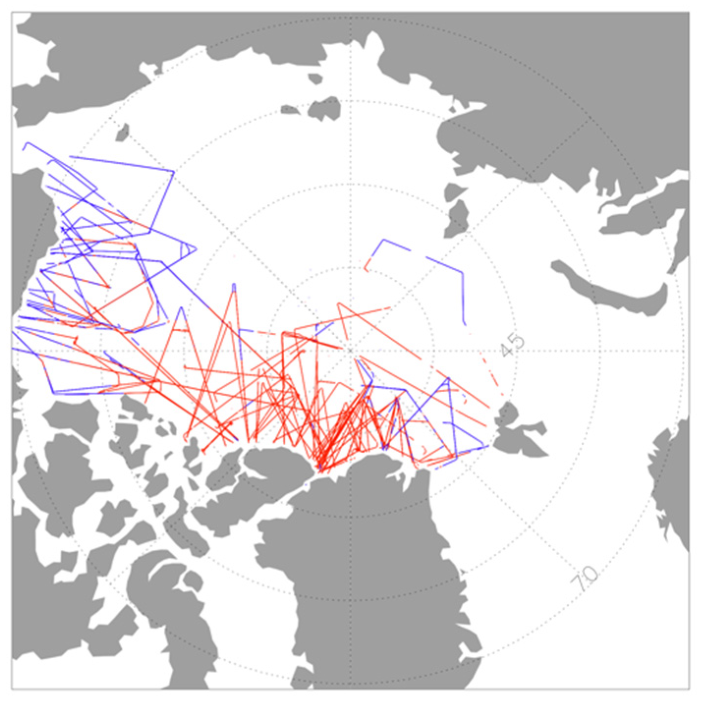
2. Data

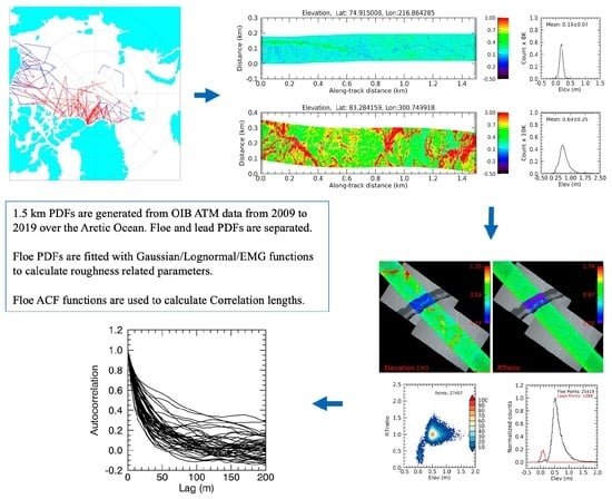
3. Methods and Analysis
3.1. Candidate Models for the PDFs
3.1.1. Gaussian Distribution
3.1.2. Lognormal Distribution
3.1.3. EMG Distribution
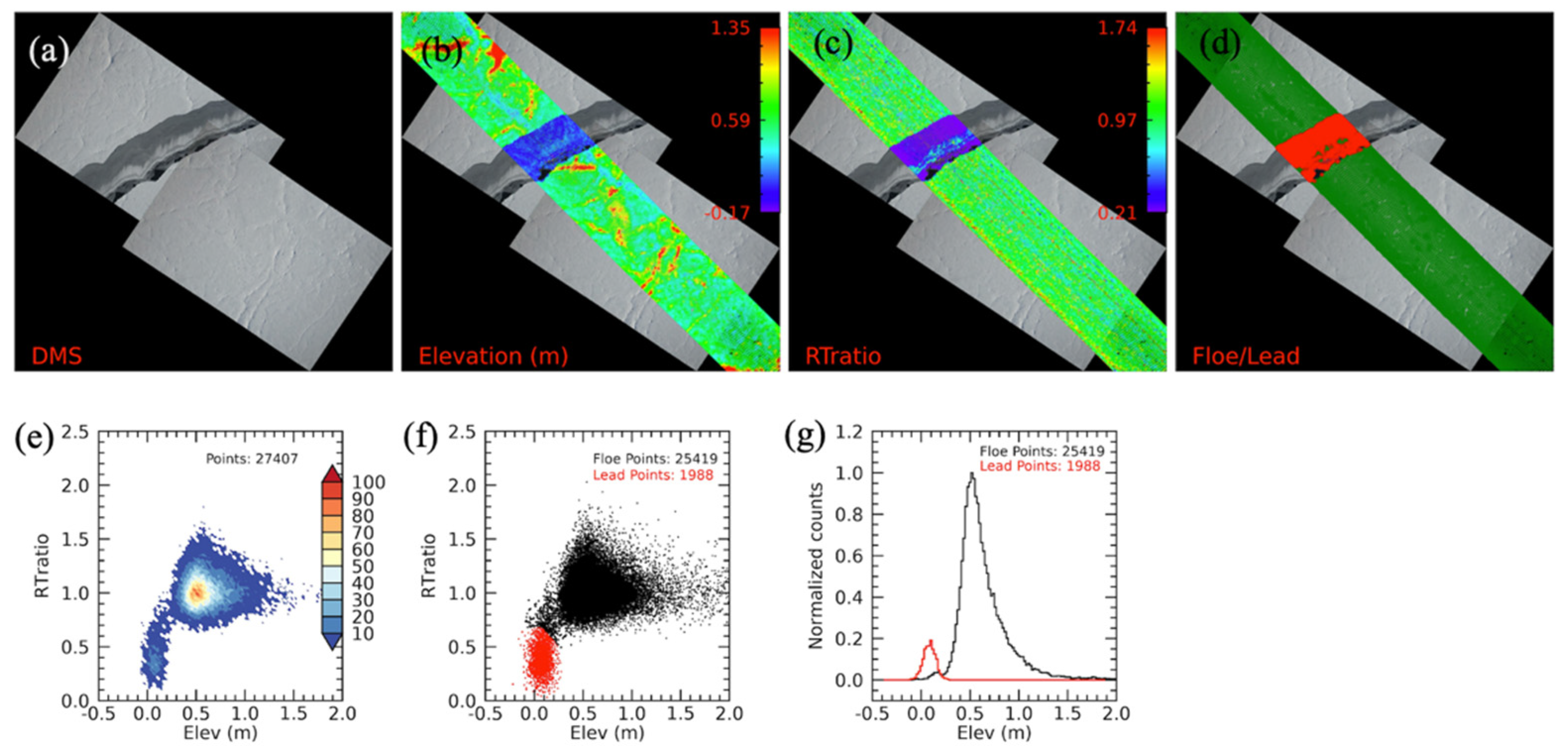
3.2. Cluster Analysis to Distinguish Floe Heights from Lead Heights
3.3. Weakly Stationary Surface Processes
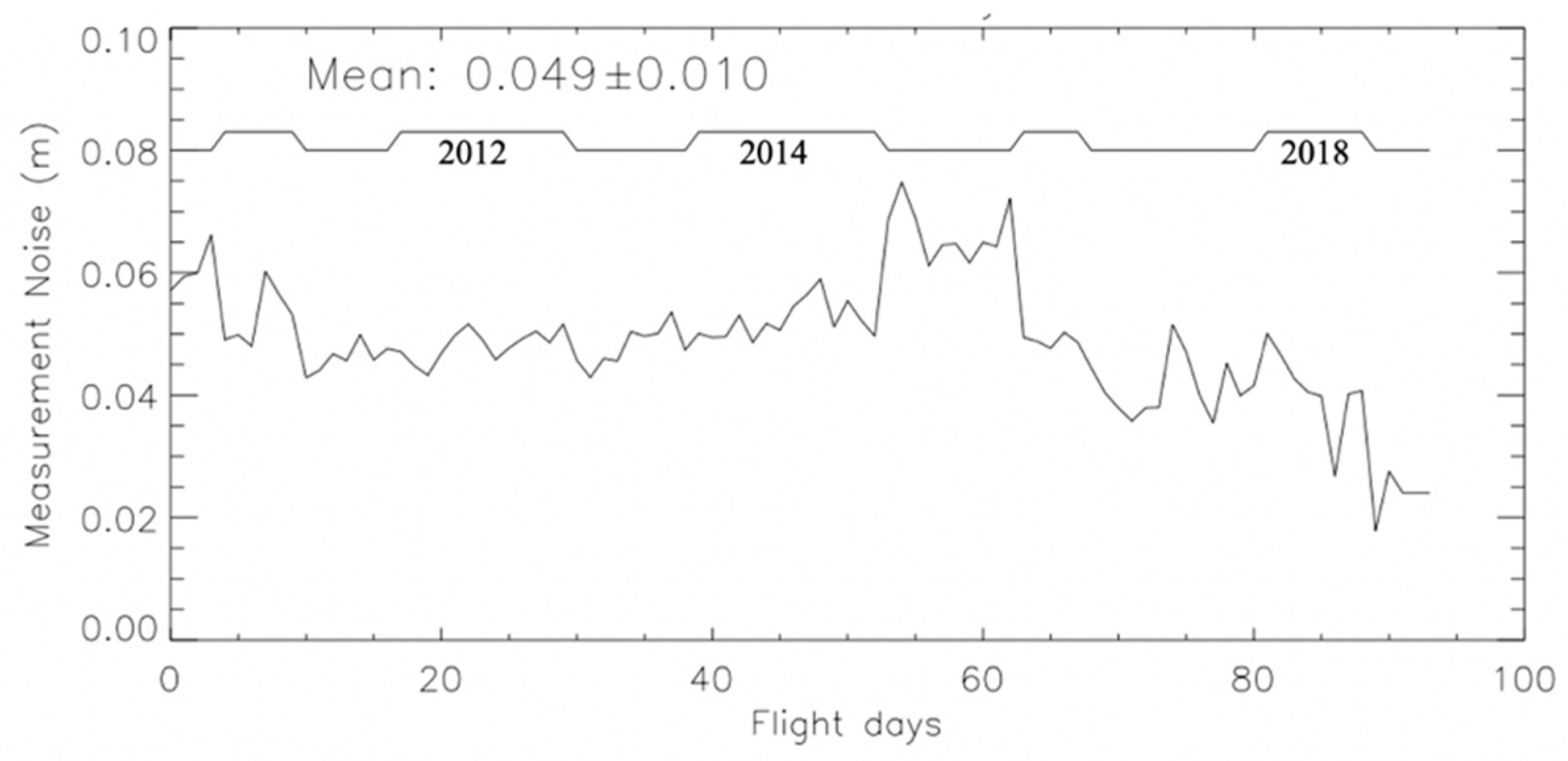
3.4. ATM Measurement Noise
3.5. Local Anisotropy and Segment-Scale Isotropy
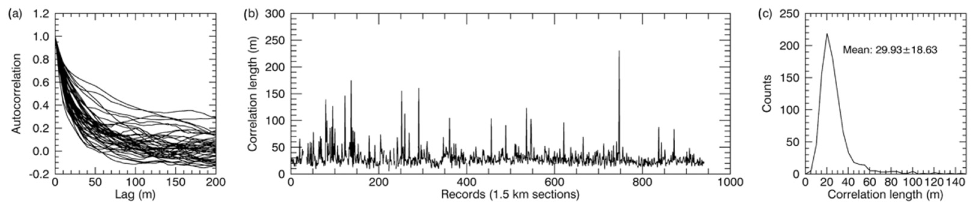
3.6. Correlation Length Estimation
4. Results and Discussion
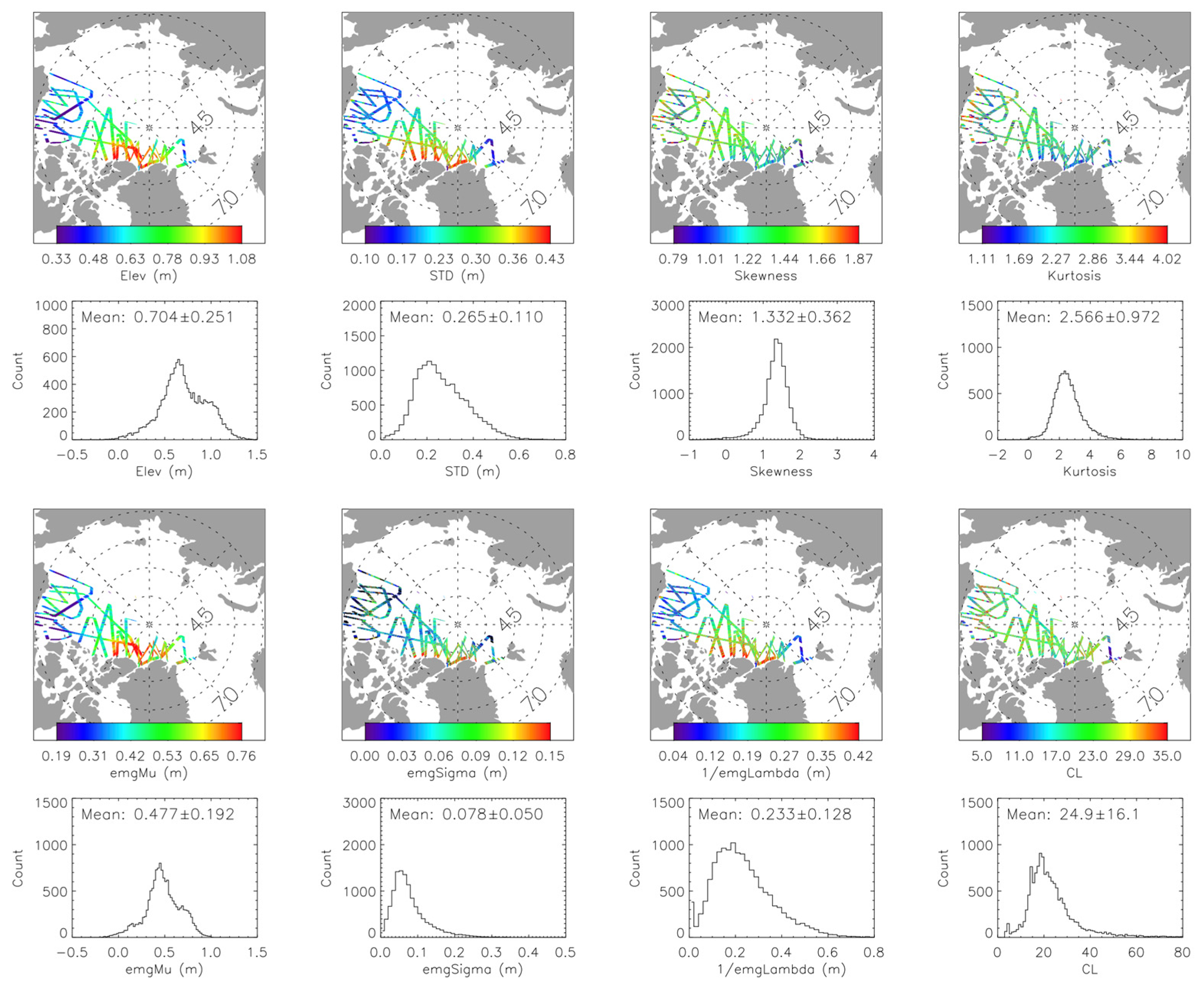
4.1. Elevation PDF Model Fitting
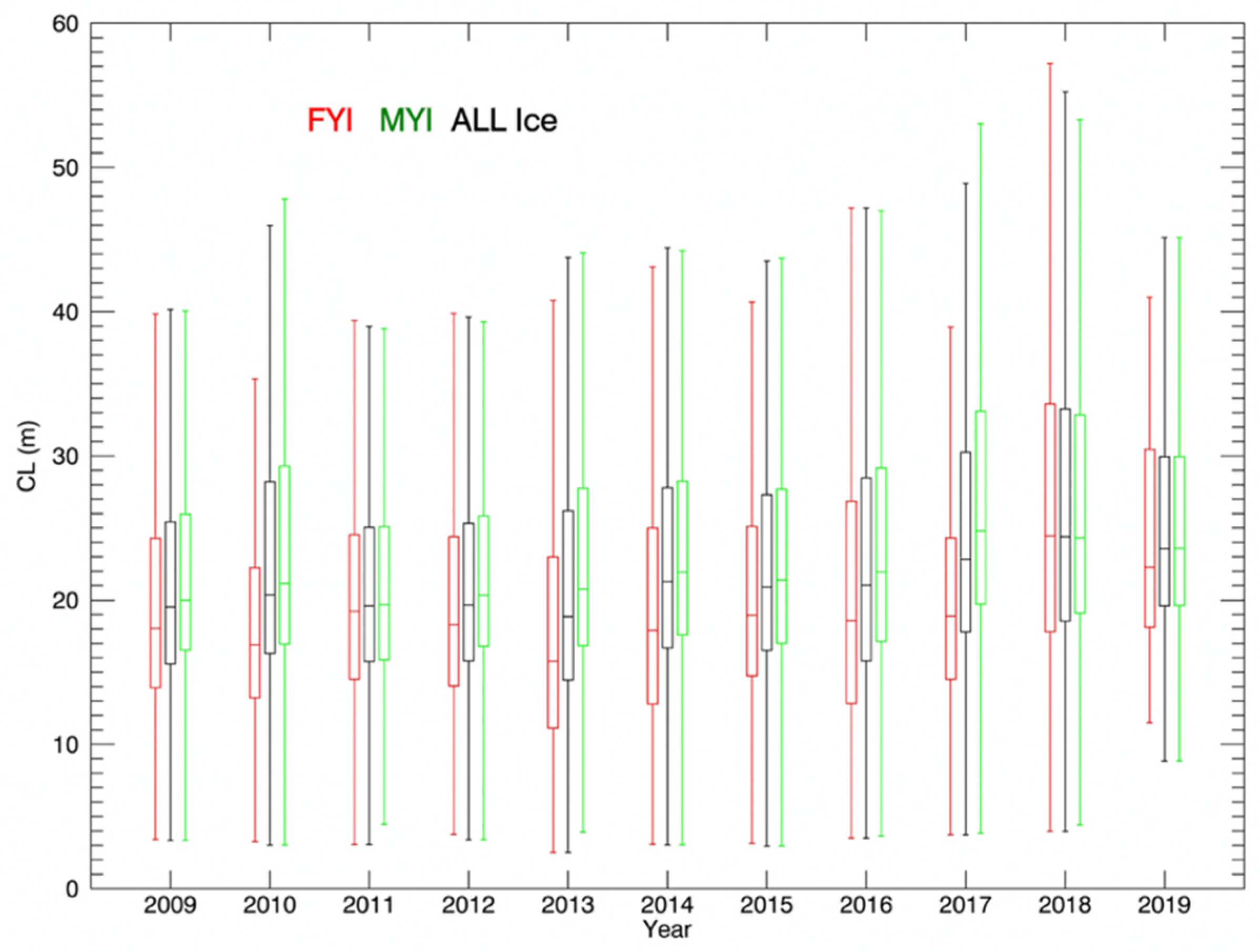
4.2. CL Distribution over the Arctic
4.3. Snow Depth Impact and Future Work
5. Conclusions
Author Contributions
Funding
Data Availability Statement
Acknowledgments
Conflicts of Interest
References
- Kwok, R.; Petty, A.; Cunningham, G.F.; Hancock, D.W.; Ivanoff, A.; Wimert, J.T.; Bagnardi, M.; Kurtz, N. Algorithm Theoretical Basis Document (ATBD) For Sea Ice Products. In ICESat-2 Algorithm Theoretical Basis Document, Version 4; NASA Goddard Space Flight Center: Greenbelt, MD, USA, 2021. [Google Scholar]
- Brenner, A.C.; Zwally, H.J.; Bentley, C.R.; Csatho, B.M.; Harding, D.J.; Hufton, M.A.; Minster, J.B.; Roberts, L.; Saba, J.L.; Thomas, R.H.; et al. Derivation of Range and Range Distributions from Laser Pulse Waveform Analysis for Surface Elevations, Roughness, Slope, and Vegetation Heights. In ICESat Algorithm Theoretical Basis Document, Version 5; NASA Goddard Space Flight Center: Greenbelt, MD, USA, 2011. [Google Scholar]
- Wingham, D.J.; Francis, C.R.; Baker, S.; Bouzinac, C.; Brockley, D.; Cullen, R.; Chateau-Thierry, P.; Laxon, S.W.; Mallow, U.; Mavrocordatos, C.; et al. Cryosat: A mission to determine the fluctuations in Earth’s land and marine ice fields. Adv. Space Res. 2006, 37, 841–871. [Google Scholar] [CrossRef]
- Laxon, S.W.; Giles, K.A.; Ridout, A.L.; Wingham, D.J.; Willatt, R.; Cullen, R.; Kwok, R.; Schweiger, A.; Zhang, J.; Haas, C.; et al. CryoSat-2 estimates of Arctic sea ice thickness and volume. Geophys. Res. Lett. 2013, 40, 732–737. [Google Scholar] [CrossRef] [Green Version]
- Berger, T. Satellite altimetry using ocean backscatter. IEEE Trans. Antennas Propag. 1972, 20, 295–309. [Google Scholar] [CrossRef]
- Brown, G.S. The average impulse response of a rough surface and its applications. IEEE Trans. Antennas Propag. 1977, 25, 67–74. [Google Scholar] [CrossRef]
- Tayfun, M.A. Narrow-Band Nonlinear Sea Waves. J. Geophys. Res. 1980, 85, 1548–1582. [Google Scholar] [CrossRef]
- Raney, R.K. The Delay/Dopper Radar Altimeter. IEEE Trans. Geosci. Remote Sens. 1998, 36, 1578–1588. [Google Scholar] [CrossRef]
- Egido, A.W.; Smith, H.F. Fully Focused SAR Altimetry: Theory and Applications. IEEE Trans. Geosci. Remote Sens. 2017, 55, 392–406. [Google Scholar] [CrossRef]
- Egido, A.; Smith, W.H.F. Pulse-to-Pulse Correlation Effects in High PRF Low-Resolution Mode Altimeters. IEEE Trans. Geosci. Remote Sens. 2019, 57, 2610–2617. [Google Scholar] [CrossRef]
- Landy, J.C.; Tsamados, M.; Scharien, R.K. A Facet-Based Numerical Model for Simulating SAR Altimeter Echoes from Heterogeneous Sea Ice Surfaces. IEEE Trans. Geosci. Remote Sens. 2019, 57, 4164–4180. [Google Scholar] [CrossRef] [Green Version]
- Rivas, M.B.; Maslanik, J.A.; Sonntag, J.G.; Axelrad, P. Sea Ice Roughness from Airborne LIDAR Profiles. IEEE Trans. Geosci. Remote Sens. 2006, 44, 3032–3037. [Google Scholar] [CrossRef]
- Landy, J.C.; Petty, A.A.; Tsamados, M.; Stroeve, J.C. Sea ice roughness overlooked as a key source of uncertainty in CryoSat-2 ice freeboard retrievals. J. Geophys. Res. Ocean 2020, 125, e2019JC015820. [Google Scholar] [CrossRef]
- Hughes, B.A. On the use of lognormal statistics to simulate one- and two-dimensional under-ice draft profiles. J. Geophys. Res. 1991, 96, 22101–22111. [Google Scholar] [CrossRef]
- Davis, N.; Wadhams, P. A statistical analysis of Arctic pressure ridge morphology. J. Geophys. Res. 1995, 100, 10915–10925. [Google Scholar] [CrossRef]
- Castellani, G.; Lüpkes, C.; Hendricks, S.; Gerdes, R. Variability of Arctic sea-ice topography and its impact on the atmospheric surface drag. J. Geophys. Res. Ocean 2014, 119, 6743–6762. [Google Scholar] [CrossRef]
- Krabill, W.B.; Abdalati, W.; Frederick, E.B.; Manizade, S.S.; Martin, C.F.; Sonntag, J.; Swift, R.N.; Thomas, R.H.; Yungel, J.G. Aircraft laser altimetry measurement of elevation changes of the Greenland ice sheet: Technique and accuracy assessment. J. Geodyn. 2002, 34, 357–376. [Google Scholar] [CrossRef]
- Martin, C.F.; Krabill, W.B.; Manizade, S.S.; Russell, R.L.; Sonntag, J.G.; Swift, R.N.; Yungel, J.K. Airborne Topographic Mapper Calibration Procedures and Accuracy Assessment; Technical Report NASA/TM-2012-215891; NASA Goddard Space Flight Center: Greenbelt, MD, USA, 2012. Available online: https://ntrs.nasa.gov/archive/nasa/casi.ntrs.nasa.gov/20120008479.pdf (accessed on 1 March 2022).
- Dominguez, R. IceBridge DMS L1B Geolocated and Orthorectified Images, Version 1; Technical Report updated 2018; NASA National Snow Ice Data Center Distributed Active Archive Center: Boulder, CO, USA, 2018. [Google Scholar] [CrossRef]
- Studinger, M. IceBridge ATM L1B Elevation and Return Strength, Version 2; updated 2020; NASA National Snow and Ice Data Center Distributed Active Archive Center: Boulder, CO, USA, 2020. [Google Scholar] [CrossRef]
- Krabill, W.B.; Thomas, R.H.; Martin, C.F.; Swift, R.N.; Frederick, E.B. Accuracy of airborne laser altimetry over the Greenland ice sheet. Int. J. Remote Sens. 1995, 16, 1211–1222. [Google Scholar] [CrossRef]
- Brunt, K.M.; Hawley, R.L.; Lutz, E.R.; Studinger, M.; Sonntag, J.G.; Hofton, M.A.; Andrews, L.C.; Neumann, T.A. Assessment of NASA airborne laser altimetry data using ground-based GPS data near Summit Station, Greenland. Cryosphere 2017, 11, 681–692. [Google Scholar] [CrossRef] [Green Version]
- Andersen, O.B.; Stenseng, L.; Piccioni, G.; Knudsen, P. The DTU15 MSS (Mean Sea Surface) and DTU15LAT (Lowest Astronomical Tide) Reference Surface. In Proceedings of the ESA Living Planet Symposium, Prague, Czech Republic, 9–13 May 2016; Available online: https://ftp.space.dtu.dk/pub/DTU15/DOCUMENTS/MSS/DTU15MSS+LAT.pdf (accessed on 1 March 2022).
- Andersen, O.B.; Knudsen, P. DNSC08 mean sea surface and mean dynamic topography models. J. Geophys. Res. 2009, 114, C11001. [Google Scholar] [CrossRef]
- Smith, W.H.F. Direct conversion of latitude and height from one ellipsoid to another. J. Geod. 2022, in press. [Google Scholar] [CrossRef]
- Yi, D.; Harbeck, J.P.; Manizade, S.S.; Kurtz, N.T.; Studinger, M.; Hofton, M. Arctic Sea Ice Freeboard Retrieval with Waveform Characteristics for NASA’s Airborne Topographic Mapper (ATM) and Land, Vegetation, and Ice Sensor (LVIS). IEEE Trans. Geosci. Remote Sens. 2015, 53, 1403–1410. [Google Scholar] [CrossRef]
- Aaboe, S.; Breivik, L.-A.; Sorense, A.; Eastwood, S.; Lavergne, T. Ocean & Sea Ice SAF, Global Sea Ice Edge and Type, Product User’s Manual, OSI-402-c & OSI-403-c, Version 2.3; Norwegian Meteorological Institute: Oslo, Norway, 2018.
- Exponentially Modified Gaussian Distribution. Available online: https://en.wikipedia.org/wiki/Exponentially_modified_Gaussian_distribution (accessed on 1 March 2021).
- Onana, V.D.P.; Kurtz, N.T.; Farrell, S.L.; Koenig, L.S.; Studinger, M.; Harbeck, J.P. A sea-ice lead detection algorithm for use with high resolution airborne visible imagery. IEEE Trans. Geosci. Remote Sens. 2013, 51, 38–56. [Google Scholar] [CrossRef]
- CLUSTER. Available online: https://www.l3harrisgeospatial.com/docs/cluster.html (accessed on 15 March 2021).
- Everitt, B.S. Cluster Analysis; Halsted Press: New York, NY, USA, 1993; ISBN 0-470-22043-0. [Google Scholar]
- MacGregor, J.A.; Boisvert, L.N.; Medley, B.; Petty, A.A.; Harbeck, J.P.; Bell, R.E.; Blair, J.B.; Blanchard-Wrigglesworth, E.; Buckley, E.M.; Christoffersen, M.S.; et al. The scientific legacy of NASA’s Operation IceBridge. Rev. Geophys. 2021, 59, e2020RG000712. [Google Scholar] [CrossRef]
- Church, E.L. Comments on the Correlation Length. In Proceedings of the SPIE 0680, Surface Characterization and Testing, Bay Point, FL, USA, 23 March 1987. [Google Scholar] [CrossRef]
- Cavalieri, D.J.; Markus, T.; Maslanik, J.; Sturm, M.; Lobl, E. March 2003 EOS Aqua AMSR-E Arctic Sea Ice Field Campaign. IEEE Trans. Geosci. Remote Sens. 2006, 44, 3003–3008. [Google Scholar] [CrossRef]
- Willatt, R.; Laxon, S.; Giles, K.; Cullen, R.; Haas, C.; Helm, V. Ku-band radar penetration into snow cover Arctic sea ice using airborne data. Ann. Glaciol. 2011, 52, 197–205. [Google Scholar] [CrossRef] [Green Version]
- Doble, M.; Skourup, H.; Wadhams, P.; Geiger, C. The relation between Arctic sea ice surface elevation and draft: A case study using coincident AUV sonar and air-borne scanning laser. J. Geophys. Res. 2011, 116, C00E03. [Google Scholar] [CrossRef] [Green Version]
- Iacozza, J.; Barber, D. An examination of the distribution of snow on sea-ice. Atmos. Ocean 1999, 37, 21–51. [Google Scholar] [CrossRef]
- Kurtz, N.T.; Farrell, S.L.; Studinger, M.; Galin, N.; Harbeck, J.P.; Lindsay, R.; Onana, V.D.; Panzer, B.; Sonntag, J.G. Sea ice thickness, freeboard, and snow depth products from Operation IceBridge air-borne data. Cryosphere 2013, 7, 1035–1056. [Google Scholar] [CrossRef] [Green Version]


| Year | FYI CL (m) | MYI CL (m) | All Ice CL (m) |
|---|---|---|---|
| 2009 | 21.51 ± 14.33 | 23.28 ± 12.28 | 22.66 ± 13.06 |
| 2010 | 19.78 ± 13.88 | 26.47 ± 18.71 | 25.45 ± 18.22 |
| 2011 | 22.12 ± 15.44 | 22.42 ± 12.25 | 22.39 ± 12.58 |
| 2012 | 20.90 ± 12.06 | 22.99 ± 12.01 | 22.23 ± 12.07 |
| 2013 | 21.10 ± 19.80 | 25.12 ± 15.68 | 23.37 ± 17.70 |
| 2014 | 20.86 ± 15.85 | 25.60 ± 15.95 | 24.87 ± 16.09 |
| 2015 | 21.80 ± 13.40 | 24.66 ± 14.80 | 24.13 ± 14.59 |
| 2016 | 23.18 ± 19.36 | 25.40 ± 15.99 | 24.72 ± 17.12 |
| 2017 | 21.74 ± 14.44 | 29.64 ± 18.16 | 26.85 ± 17.36 |
| 2018 | 28.92 ± 20.13 | 29.54 ± 19.29 | 29.21 ± 19.75 |
| 2019 | 29.30 ± 19.78 | 27.62 ± 15.51 | 27.67 ± 15.65 |
Publisher’s Note: MDPI stays neutral with regard to jurisdictional claims in published maps and institutional affiliations. |
© 2022 by the authors. Licensee MDPI, Basel, Switzerland. This article is an open access article distributed under the terms and conditions of the Creative Commons Attribution (CC BY) license (https://creativecommons.org/licenses/by/4.0/).
Share and Cite
Yi, D.; Egido, A.; Smith, W.H.F.; Connor, L.; Buchhaupt, C.; Zhang, D. Arctic Sea-Ice Surface Elevation Distribution from NASA’s Operation IceBridge ATM Data. Remote Sens. 2022, 14, 3011. https://doi.org/10.3390/rs14133011
Yi D, Egido A, Smith WHF, Connor L, Buchhaupt C, Zhang D. Arctic Sea-Ice Surface Elevation Distribution from NASA’s Operation IceBridge ATM Data. Remote Sensing. 2022; 14(13):3011. https://doi.org/10.3390/rs14133011
Chicago/Turabian StyleYi, Donghui, Alejandro Egido, Walter H. F. Smith, Laurence Connor, Christopher Buchhaupt, and Dexin Zhang. 2022. "Arctic Sea-Ice Surface Elevation Distribution from NASA’s Operation IceBridge ATM Data" Remote Sensing 14, no. 13: 3011. https://doi.org/10.3390/rs14133011