
A Real-Time Digital Self Interference Cancellation Method for In-Band Full-Duplex Underwater Acoustic Communication Based on Improved VSS-LMS Algorithm

 ,
,
Abstract
:1. Introduction
2. Fundamentals
2.1. System Model
2.2. IVSS-LMS Algorithm
- When the SI signal is energetically large and the far-end desired signal is overwhelmed in the high-power SI signal, or when there is no desired signal and the error mainly originates from the SI signal;
- When the filter iteration is close to the steady state, the error floating due to the arrival of the desired signal, and the error mainly comes from the desired signal;
- When the filter iteration is close to the steady state, there is no arrival of the desired signal, and the error mainly comes from the environmental noise.
Algorithm Steps
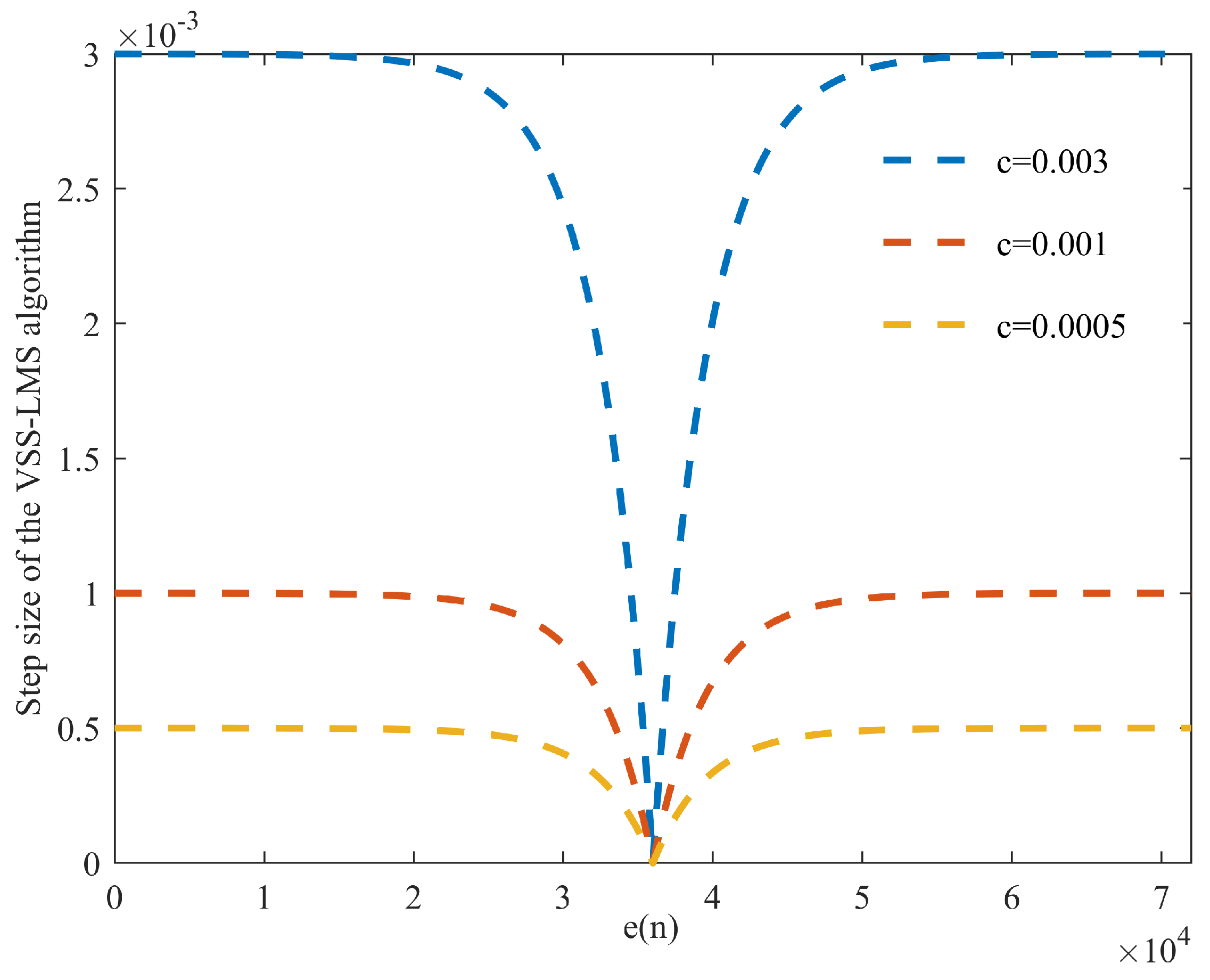
- When the error is large, , the algorithm judges that a large SI signal or sudden change in the local environment occurs in this state, so we adjusted step-size to the maximum value , in order to improve the convergence speed of the algorithm.
- When the error is close to the predetermined desired signal arrival threshold, . We adjust the step-size to the minimum value , in order to reduce the steady-state error, improve the steady-state performance, and avoid the influence of the system expectation signal on the filter, which causes a decrease in the channel estimation accuracy.
- When , the algorithm uses the Sigmoid function as a constraint that causes step-size to vary between the maximum values and minimum values for change.
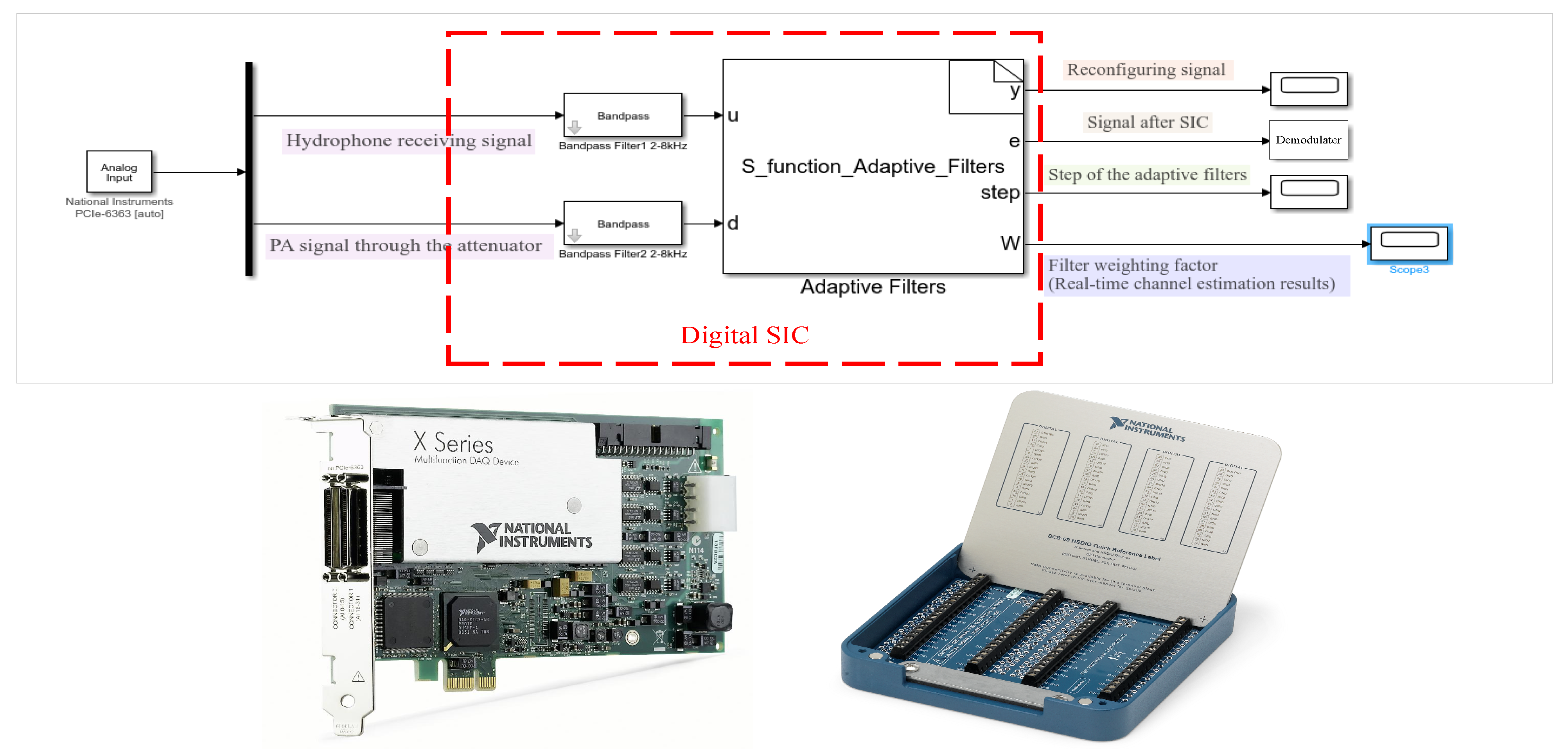
2.3. Hardware-in-Loop Simulation (HLS)
3. HLS and Experimental Results Analysis
3.1. Normalized Mean Squared Error (NMSE) Criterion
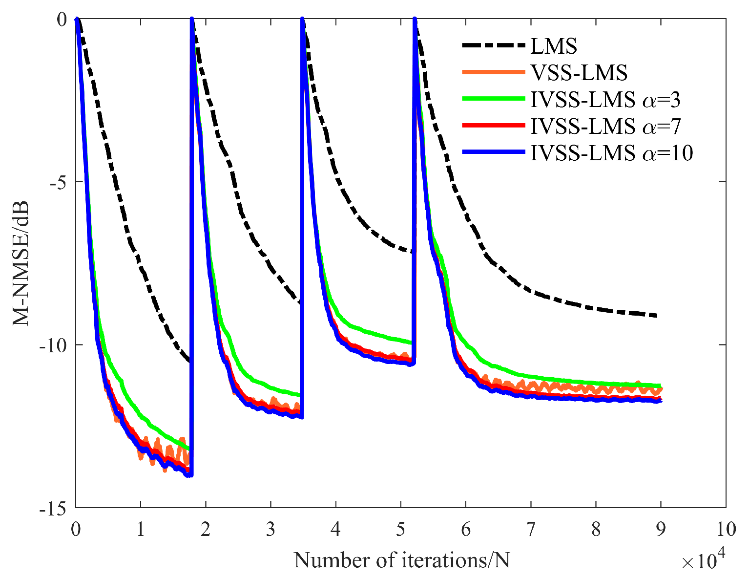
3.2. HLS Results
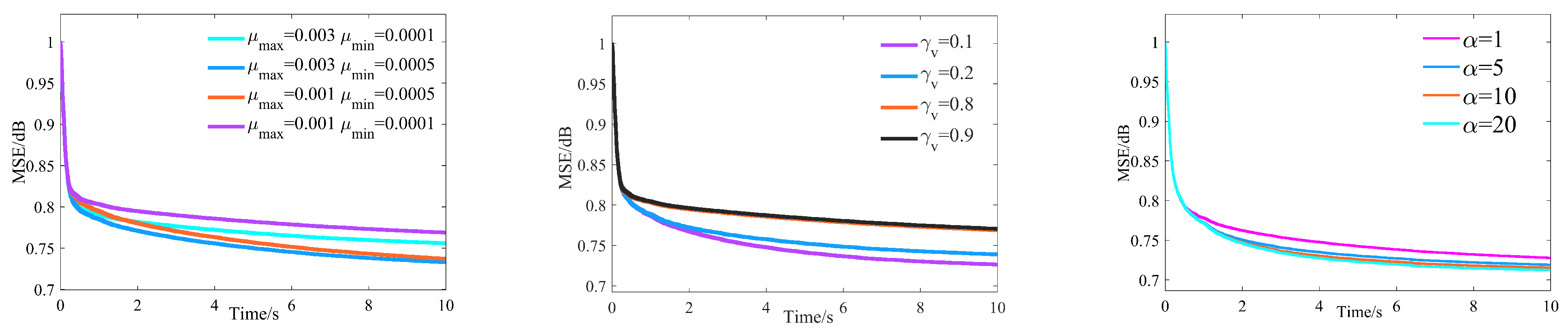
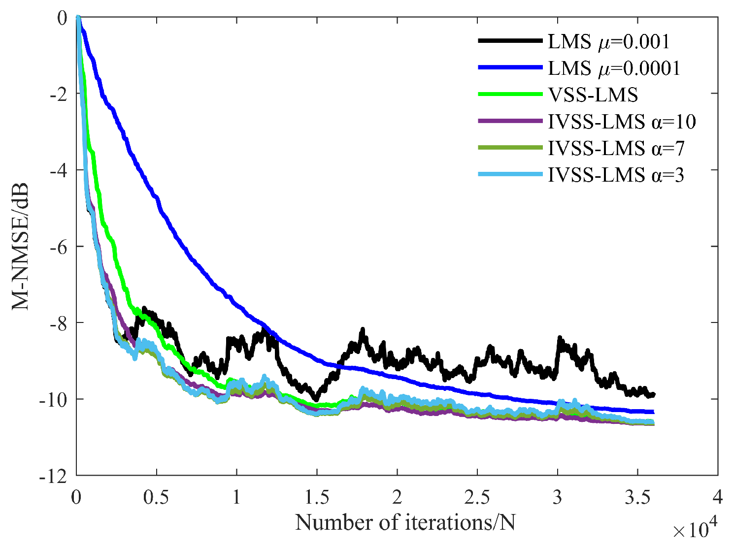
3.2.1. Optimal Parameters of IVSS-LMS
3.2.2. Practical Considerations
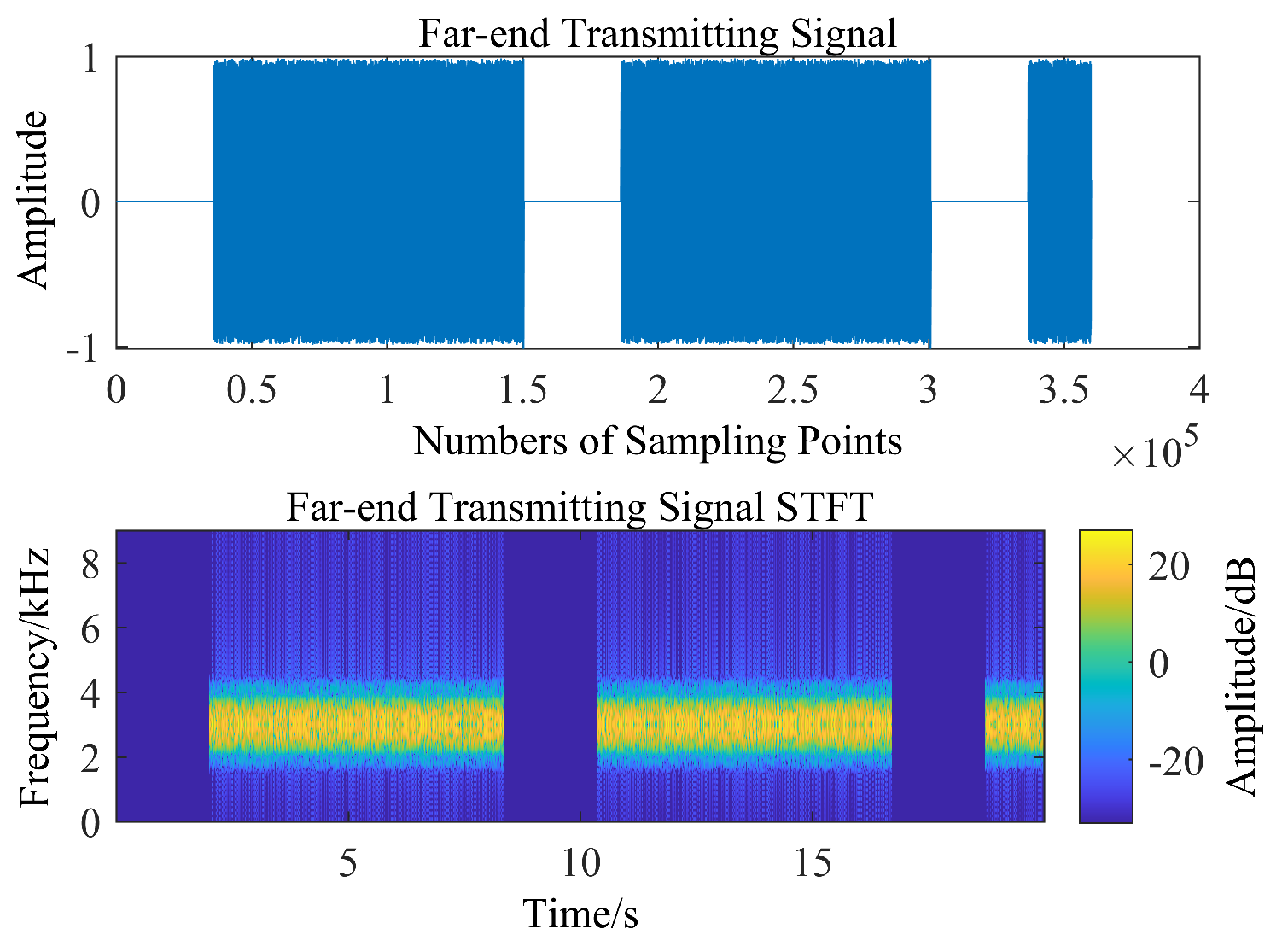
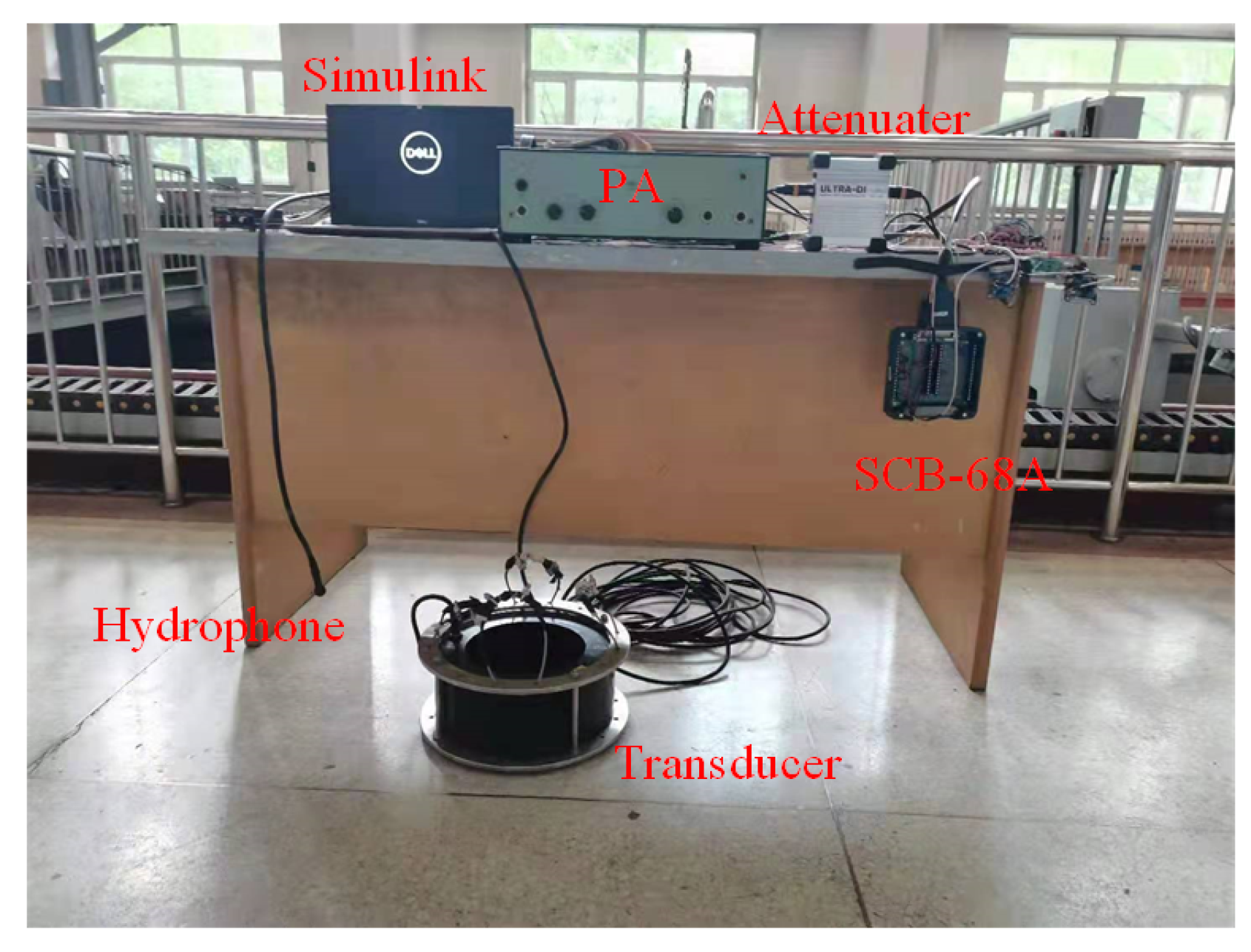
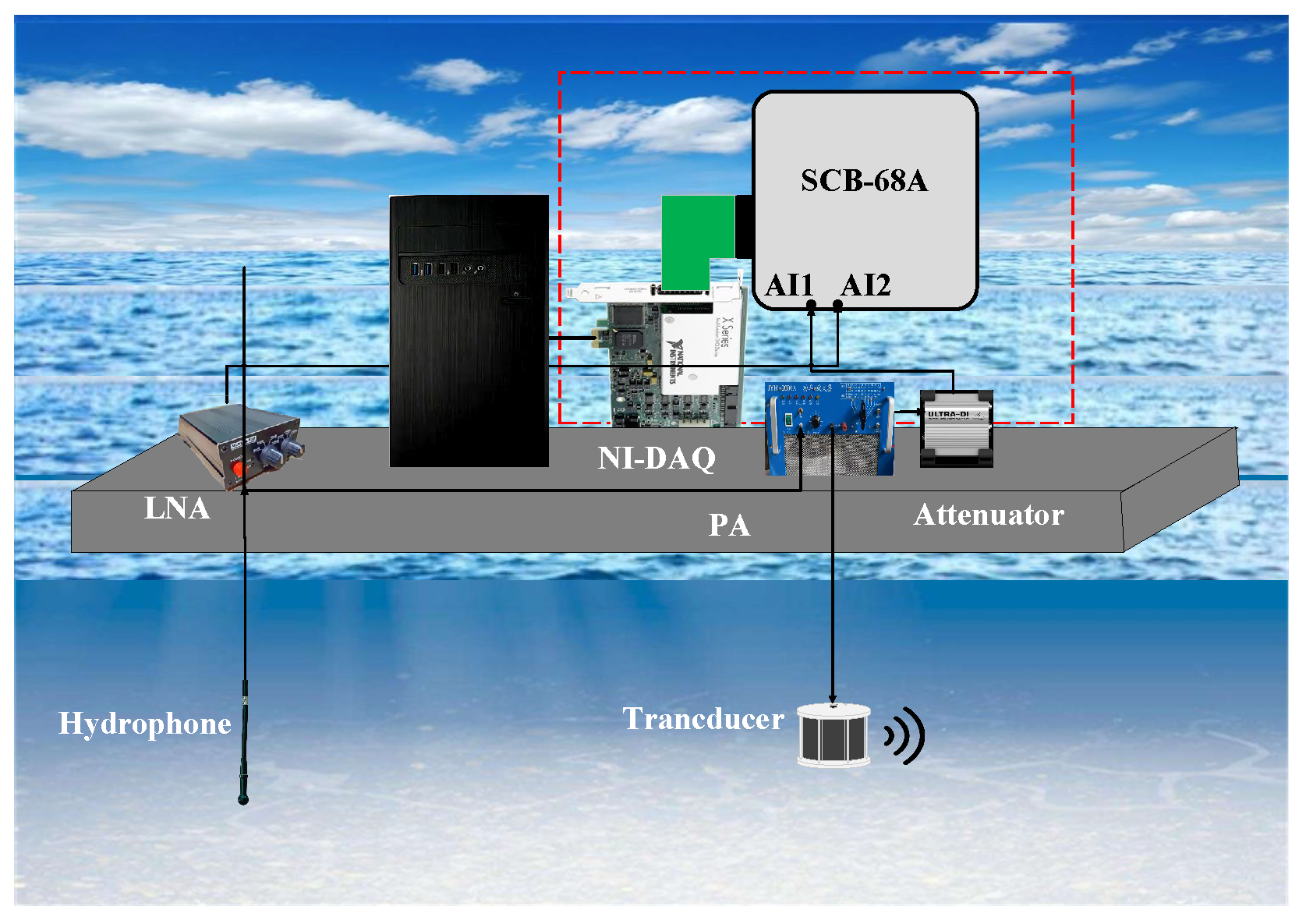
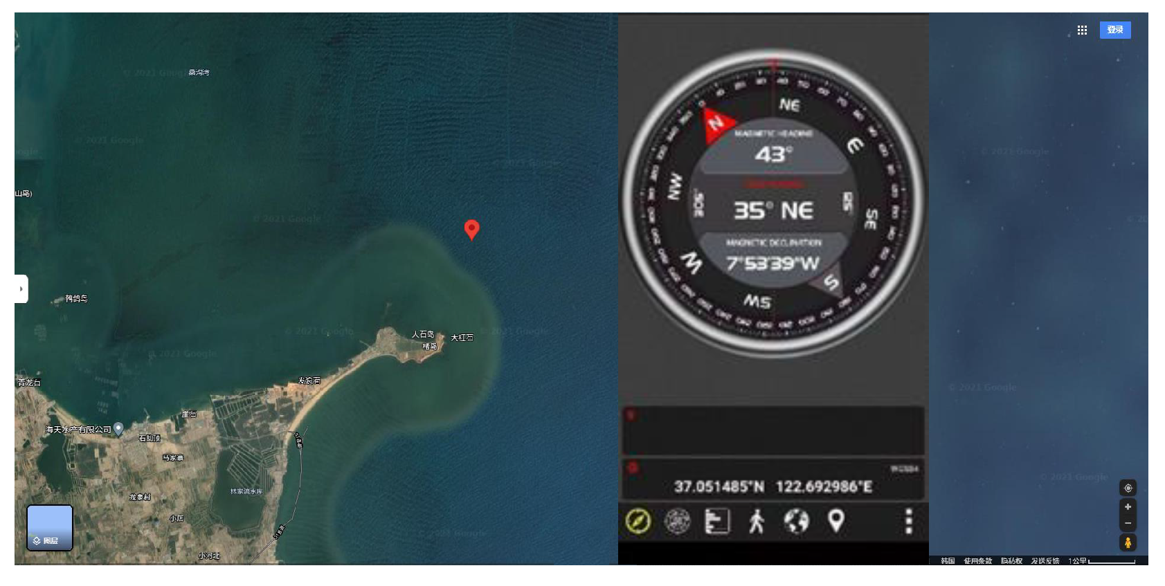
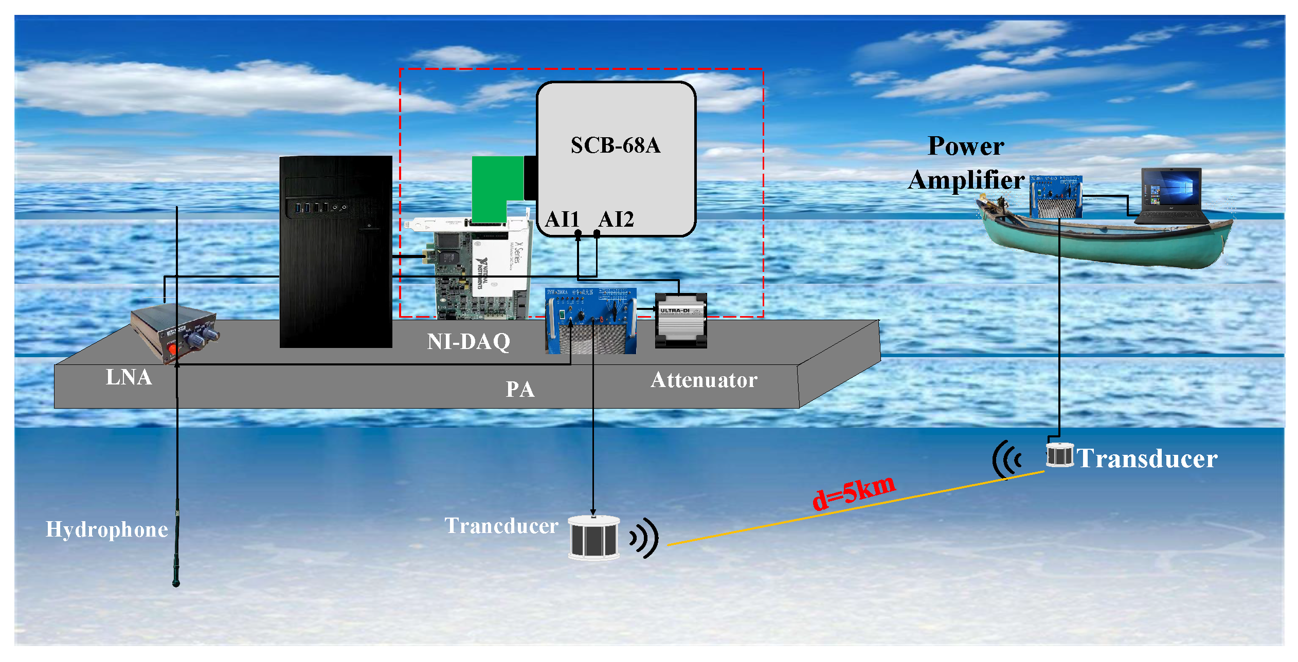
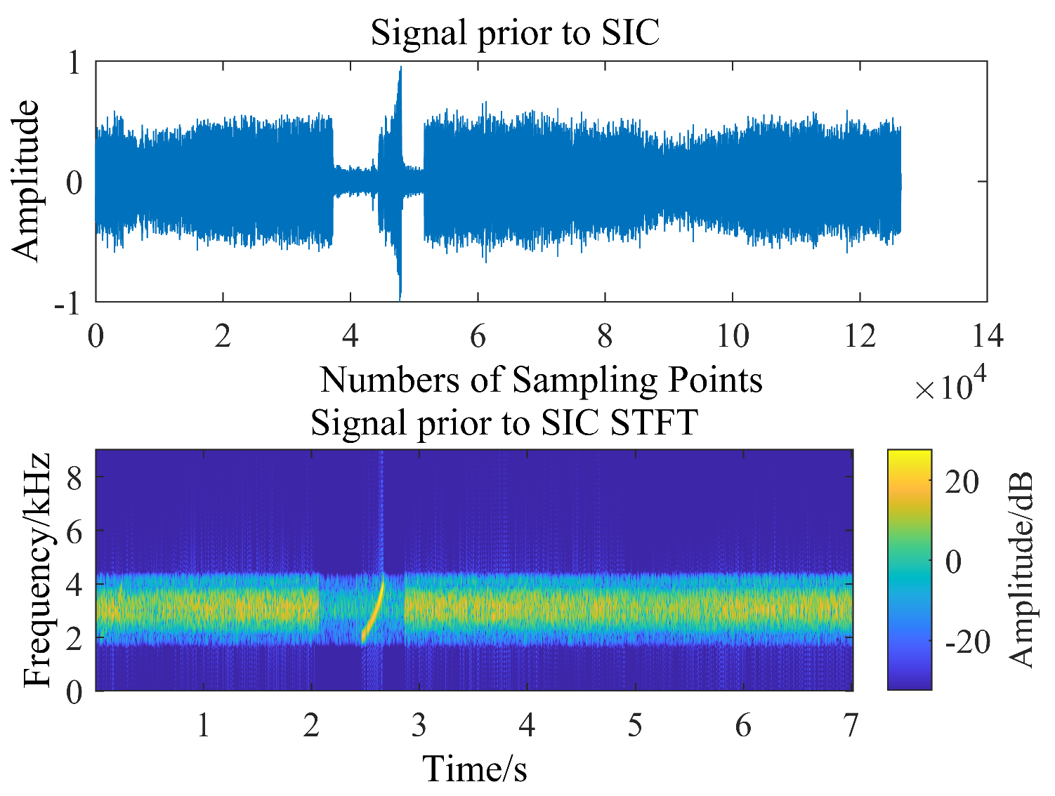
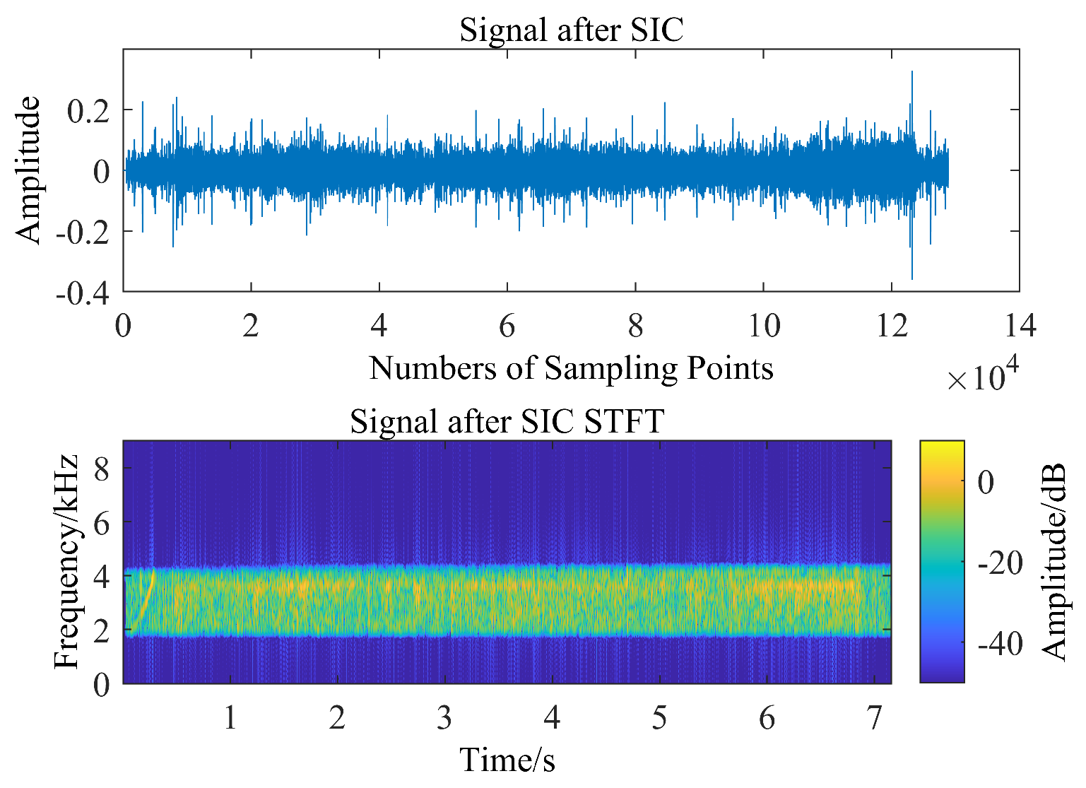
3.3. Sea Trial Test
4. Discussion
4.1. Significance of the Proposed Method
4.2. Limitations of the Proposed Method
5. Conclusions
Author Contributions
Funding
Data Availability Statement
Acknowledgments
Conflicts of Interest
References
- Stojanovic, M.; Preisig, J. Underwater acoustic communication channels: Propagation models and statistical characterization. IEEE Commun. Mag. 2009, 47, 84–89. [Google Scholar] [CrossRef]
- Chen, S.; Beach, M.A.; Mcgeehan, J.P. Division-free duplex for wireless applications. Electron. Lett. 1998, 34, 147–148. [Google Scholar] [CrossRef]
- Zhou, J.; Krishnaswamy, H. System-level analysis of phase noise in full-duplex wireless transceivers. IEEE Trans. Circuits Syst. II Express Briefs 2018, 65, 1189–1193. [Google Scholar] [CrossRef]
- Shen, L.; Henson, B.; Zakharov, Y.; Mitchell, P. Digital self-interference cancellation for full-duplex underwater acoustic systems. IEEE Trans. Circuits Syst. II Express Briefs 2019, 67, 192–196. [Google Scholar] [CrossRef] [Green Version]
- Li, S.; Lu, H.T.; Shao, S.H.; Tang, Y.X. Impact of the amount of RF self-interference cancellation on digital self-interference cancellation in full duplex communications. J. Electron. Inf. Technol. 2017, 39, 1278–1283. [Google Scholar]
- Bharadia, D.; Mcmilin, E.; Katti, S. Full duplex radios. Comput. Commun. Rev. 2013, 43, 375–386. [Google Scholar] [CrossRef]
- Hong, S.; Brand, J.; Choi, J.I.; Jain, M.; Mehlman, J.; Katti, S.; Levis, P. Applications of self-interference cancellation in 5G and beyond. IEEE Commun. Mag. 2014, 52, 114–121. [Google Scholar] [CrossRef]
- Liu, Y.; Roblin, P.; Quan, X.; Pan, W.; Shao, S.; Tang, Y. A full-duplex transceiver with two-stage analog cancellations for multipath self-interference. IEEE Trans. Microw. Theory Tech. 2017, 65, 5263–5273. [Google Scholar] [CrossRef]
- Liu, Y.; Quan, X.; Pan, W.; Tang, Y. Digitally assisted analog interference cancellation for in-band full-duplex radios. IEEE Commun. Lett. 2017, 21, 1079–1082. [Google Scholar] [CrossRef]
- Huang, X.; Le, A.T.; Guo, Y.J. ALMS loop analyses with higher-order statistics and strategies for joint analog and digital self-interference cancellation. IEEE Trans. Wirel. Commun. 2021, 20, 6467–6480. [Google Scholar] [CrossRef]
- Li, S.; Murch, R.D. An investigation into baseband techniques for single-channel fullduplex wireless communication systems. IEEE Trans. Wirel. Commun. 2014, 13, 4794–4806. [Google Scholar] [CrossRef]
- Qiao, G.; Gan, S.W.; Liu, S.Z.; Song, Q.J. Self-interference channel estimation algorithm based on maximum-likelihood estimator in in-band fullduplex underwater acoustic communication system. IEEE Access 2019, 6, 62324–62334. [Google Scholar] [CrossRef]
- Vermeulen, T.; van Liempd, B.; Hershberg, B.; Pollin, S. Real-time RF self-interference cancellation for in-band full duplex. In Proceedings of the 2015 IEEE International Symposium on Dynamic Spectrum Access Networks (DySPAN), Stockholm, Sweden, 28 September–2 October 2015; pp. 275–276. [Google Scholar]
- Kwong, R.H.; Johnston, E.W. A variable step size LMS algorithm. IEEE Trans. Signal Process. 1992, 40, 1633–1642. [Google Scholar] [CrossRef] [Green Version]
- Aboulnasr, T.; Mayyas, K. A robust variable step-size LMS-type algorithm: Analysis and simulations. IEEE Trans. Signal Process. 1997, 45, 631–639. [Google Scholar] [CrossRef]
- Pazaitis, D.I.; Constantinides, A.G. A novel kurtosis driven variable step-size adaptive algorithm. IEEE Trans. Signal Process. 1999, 47, 864–872. [Google Scholar] [CrossRef]
- Benesty, J.; Rey, H.; Vega, L.R.; Tressens, S. A nonparametric VSS NLMS algorithm. IEEE Signal Process. Lett. 2006, 13, 581–584. [Google Scholar] [CrossRef]
- Zhao, S.; Man, Z.; Khoo, S.; Wu, H.R. Variable step-size LMS algorithm with a quotient form. Signal Process 2009, 89, 67–76. [Google Scholar] [CrossRef]
- Hwang, J.K.; Li, Y.P. A gradient-based variable step size scheme for kurtosis of estimated error. IEEE Signal Process. Lett. 2010, 17, 331–334. [Google Scholar] [CrossRef]
- Huang, H.C.; Lee, J. A new variable step-size NLMS algorithm and its performance analysis. IEEE Trans. Signal Process. 2012, 60, 2055–2060. [Google Scholar] [CrossRef]
- Shin, H.C.; Sayed, A.H.; Song, W.J. Variable step-size NLMS and affine projection algorithms. IEEE Signal Process. Lett. 2004, 11, 132–135. [Google Scholar] [CrossRef]
- Mandic, D.P. A generalized normalized gradient descent algorithm. IEEE Signal Process. Lett. 2004, 11, 115–118. [Google Scholar] [CrossRef]
- Huang, B.Y.; Xiao, Y.G.; Ma, Y.P.; Wei, G.; Sun, J.W. A simplified variable step-size LMS algorithm for Fourier analysis and its statistical properties. Signal Process. 2015, 117, 69–81. [Google Scholar] [CrossRef]
- Choi, Y.S.; Shin, H.C.; Song, W.J. Robust regularization for nor-malized LMS algorithms. IEEE Trans. Circuits Syst. II Express Briefs 2006, 53, 627–631. [Google Scholar] [CrossRef]
- Jalal, B.; Yang, X.; Liu, Q.; Long, T.; Sarkar, T.K. Fast and robust variable-step-size LMS algorithm for adaptive beamforming. IEEE Antennas Wirel. Propag. Lett. 2020, 19, 1206–1210. [Google Scholar] [CrossRef]
- Garg, R.; Kohli, A.K. Parameter estimation and tracking of sinusoid using variable-step-size LMS algorithms. Optik 2016, 127, 10953–10960. [Google Scholar] [CrossRef]
- Kohli, A.K.; Sharma, J. Nonlinear acoustic echo canceller to combat sigmoid-type nonlinearities under noisy environment. Wirel. Pers. Commun. 2020, 114, 3489–3506. [Google Scholar] [CrossRef]
- Sui, Z.P.; Yan, S.F. Noise-robust variable-step LMS algorithm and its application in OFDM underwater acoustic channel equalization. Syst. Eng. Electron. Technol. 2020, 42, 1605–1613. [Google Scholar]
- Qiao, G.; Zhao, Y.J.; Liu, S.Z.; Ahmed, N. The effect of acoustic-shell coupling on near-end self-interference signal of in-band full-duplex underwater acoustic communication modem. In Proceedings of the 2020 17th International Bhurban Conference on Applied Sciences and Technology (IBCAST)), Islamabad, Pakistan, 14–18 January 2020; pp. 606–610. [Google Scholar]


| 1 Algorithm initialization |
|---|
|
| 2 Parameter Settings |
|
| 3 Loop Iteration |
|
Publisher’s Note: MDPI stays neutral with regard to jurisdictional claims in published maps and institutional affiliations. |
© 2022 by the authors. Licensee MDPI, Basel, Switzerland. This article is an open access article distributed under the terms and conditions of the Creative Commons Attribution (CC BY) license (https://creativecommons.org/licenses/by/4.0/).
Share and Cite
Lu, Y.; Qiao, G.; Yang, C.; Zhao, Y.; Yang, G.; Li, H. A Real-Time Digital Self Interference Cancellation Method for In-Band Full-Duplex Underwater Acoustic Communication Based on Improved VSS-LMS Algorithm. Remote Sens. 2022, 14, 2924. https://doi.org/10.3390/rs14122924
Lu Y, Qiao G, Yang C, Zhao Y, Yang G, Li H. A Real-Time Digital Self Interference Cancellation Method for In-Band Full-Duplex Underwater Acoustic Communication Based on Improved VSS-LMS Algorithm. Remote Sensing. 2022; 14(12):2924. https://doi.org/10.3390/rs14122924
Chicago/Turabian StyleLu, Yinheng, Gang Qiao, Chenlu Yang, Yunjiang Zhao, Guang Yang, and Huizhe Li. 2022. "A Real-Time Digital Self Interference Cancellation Method for In-Band Full-Duplex Underwater Acoustic Communication Based on Improved VSS-LMS Algorithm" Remote Sensing 14, no. 12: 2924. https://doi.org/10.3390/rs14122924