
Landslide Deformation Extraction from Terrestrial Laser Scanning Data with Weighted Least Squares Regularization Iteration Solution

 ,
,
Abstract
:
1. Introduction
2. Methodology
2.1. PCR of Multi-Period Point Cloud Data
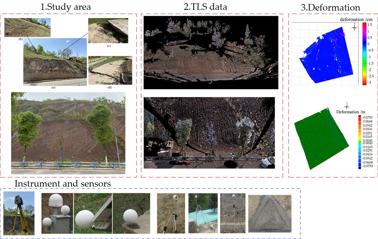
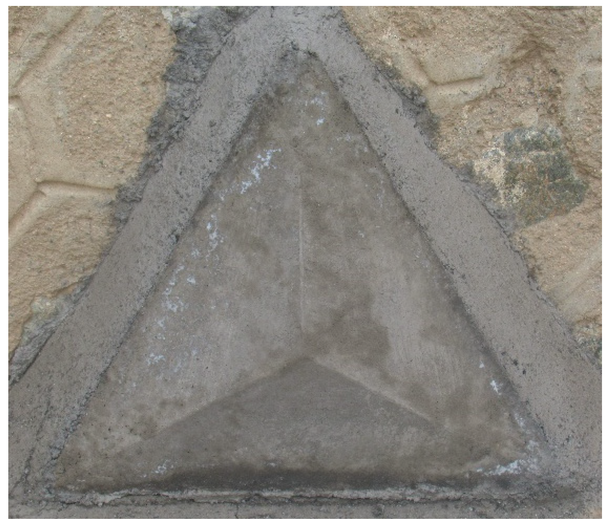
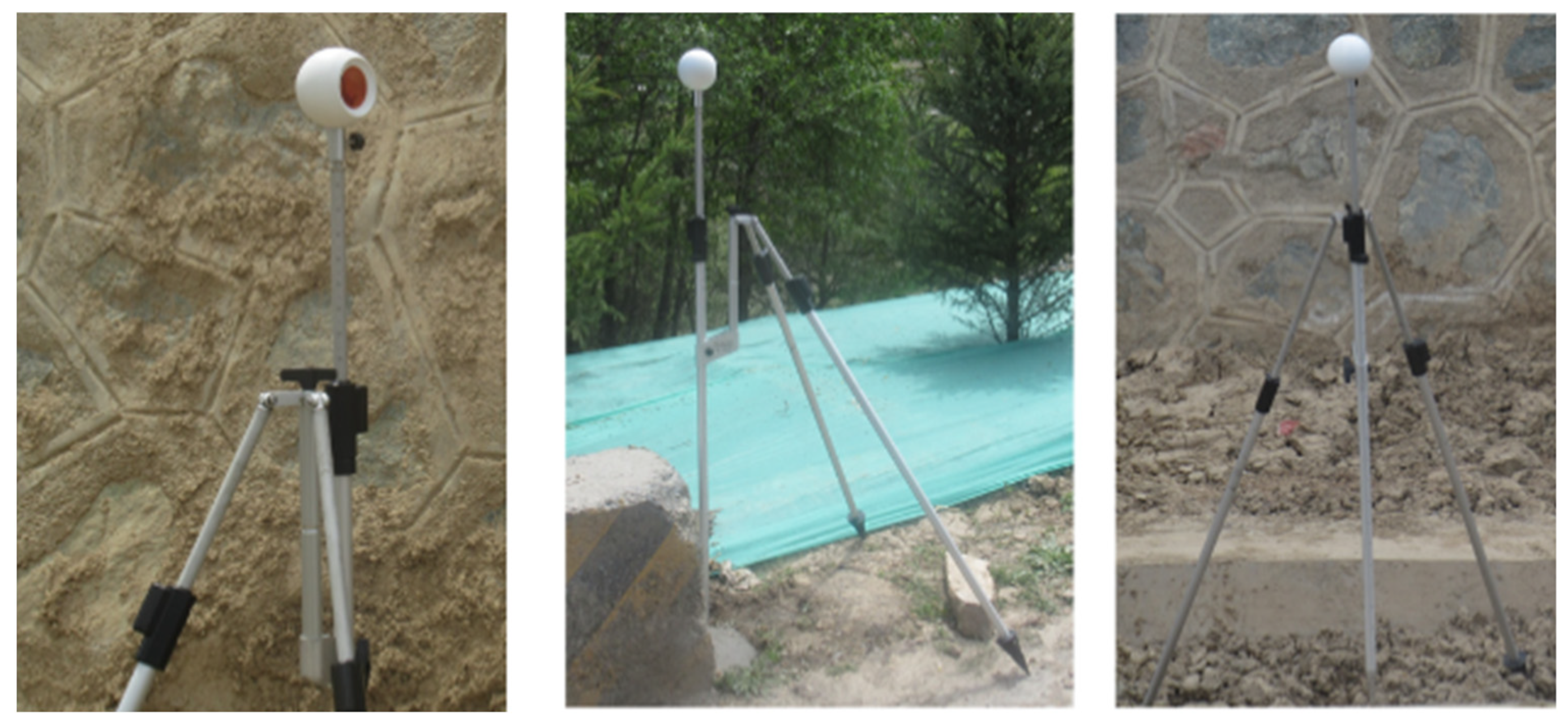
2.1.1. PCR Based on Triangular Pyramid Target
- (1)
- Setting up the matching point correspondence of two point sets,where , , is the argument of iteration k − 1.
- (2)
- The new rotation matrices and shift vectors are computed by minimizing the square distance [40],
2.1.2. PCR Based on Total Station Orientation
2.2. Landslide DTM Using the Weighted Least Squares Regularization Solution
- (1)
- Taking as the x-axis coordinate and as the y-axis coordinate, we get multiple sets of coordinate points (, ),
- (2)
- These coordinate points are fitted to a curve similar to L shape, and the value corresponding to the point with the largest curvature is used as the estimation of the regularization parameter.
- (1)
- The LS solution is used as the RWLS initial value of iteration;
- (2)
- Compute the cofactor matrix ;
- (3)
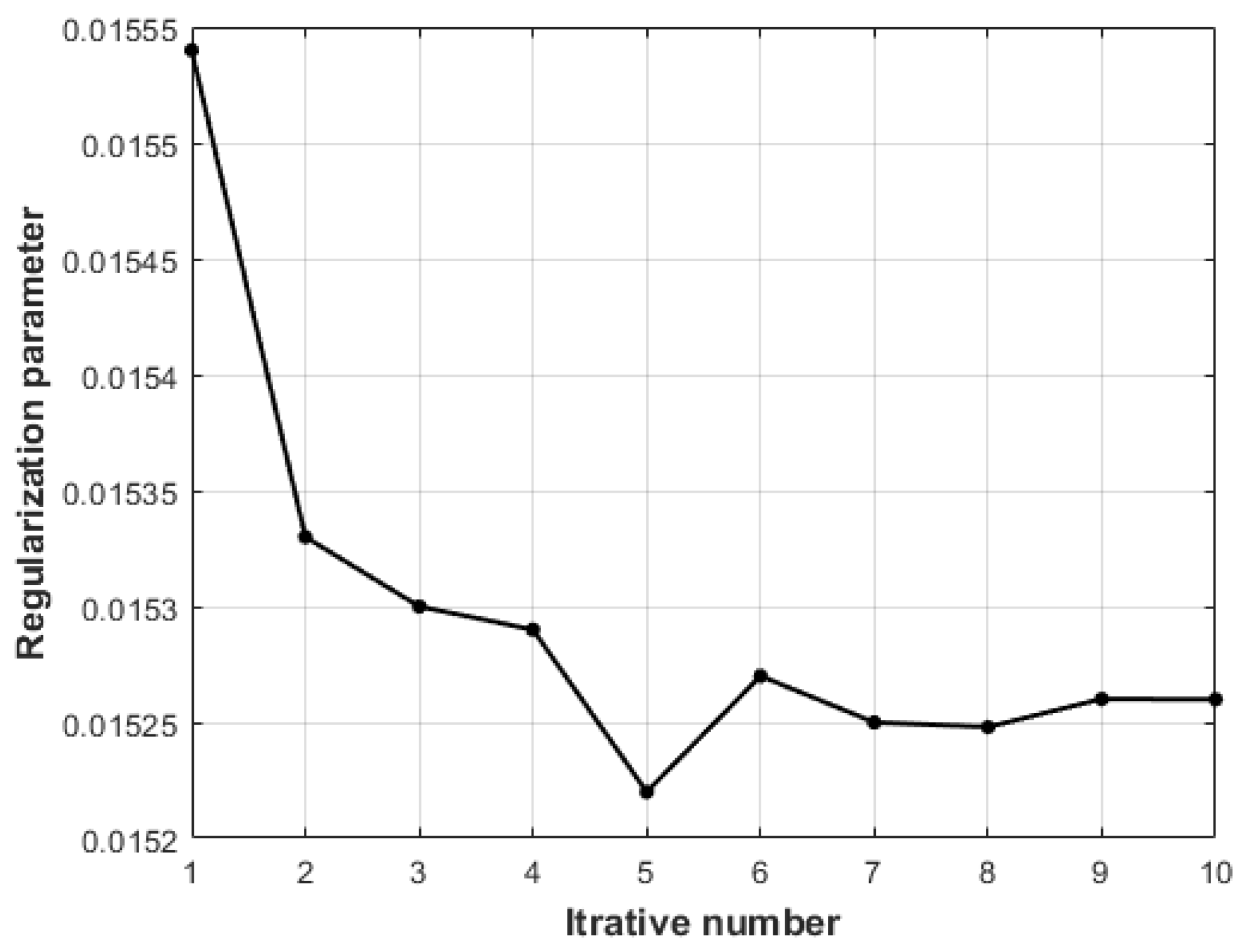
- The regularization parameter is obtained by L curve method;
- (4)
- The iterative formula is as follows:
- (5)
- Repeat steps (2)–(4) until the value of the parameter subtraction is smaller than the threshold,where is defined as 10−10 in this paper.
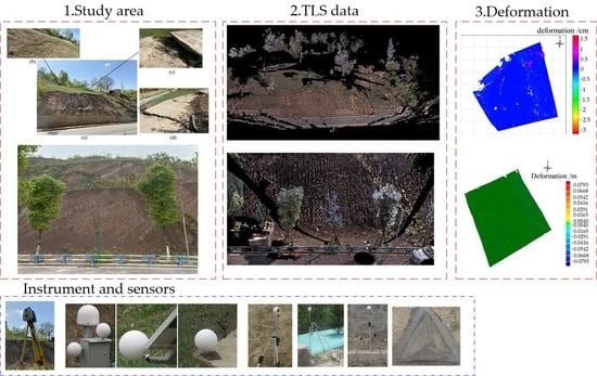
3. Experiments Data
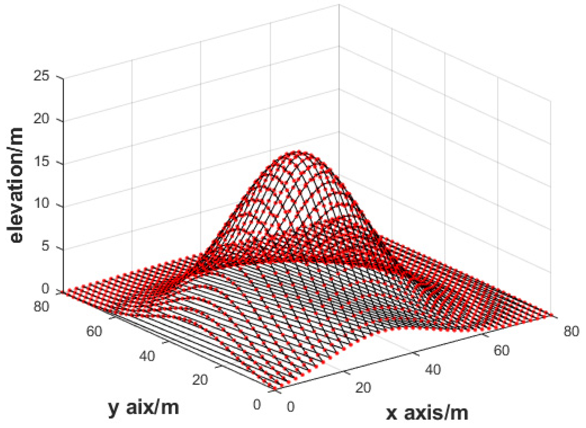
3.1. Simulation Experiment
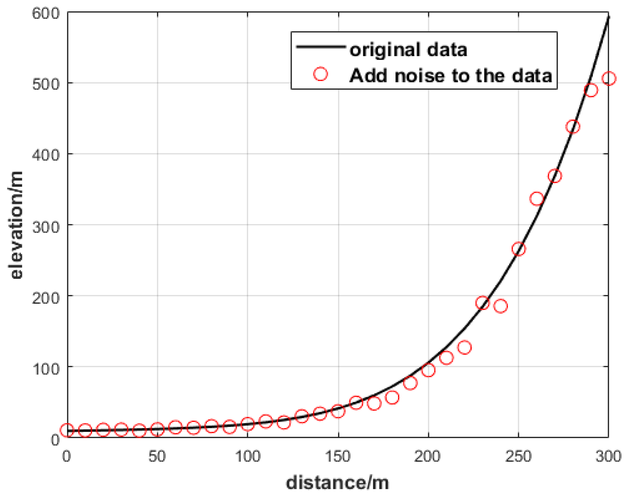
3.1.1. Simulation Experiment I: GNSS Elevation Point Disturbed by Multiplicative Error
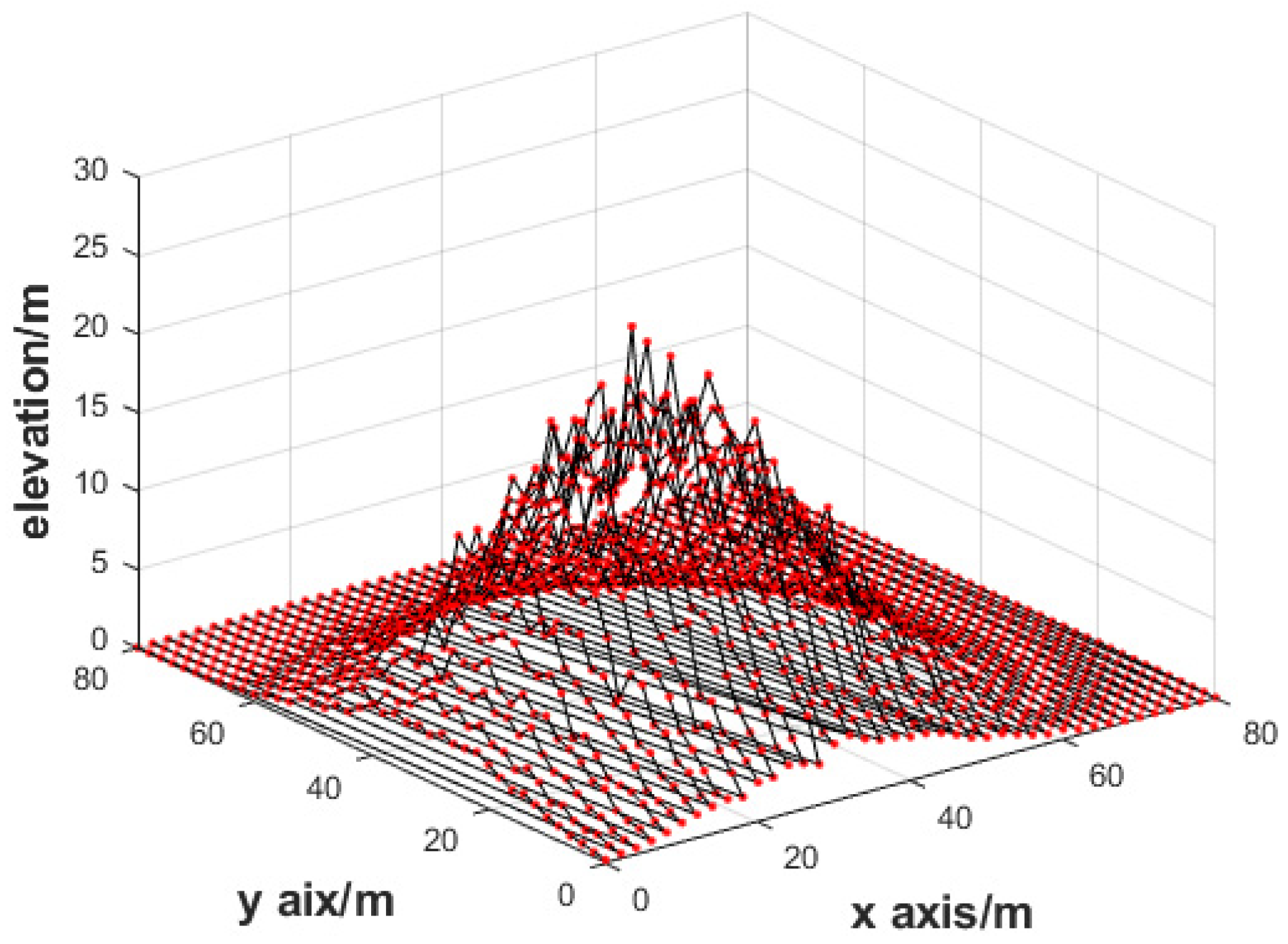
3.1.2. Simulation Experiment II
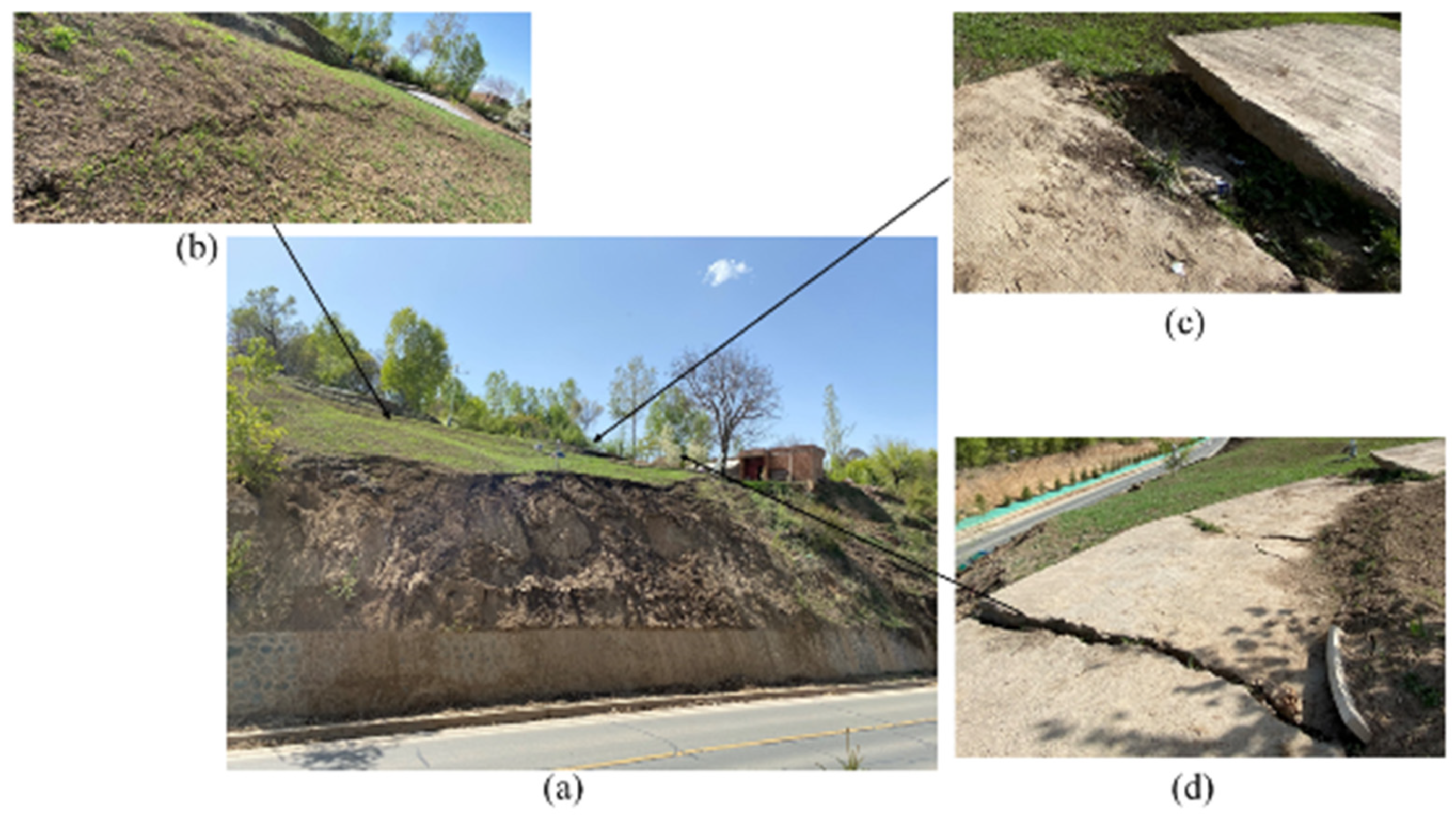
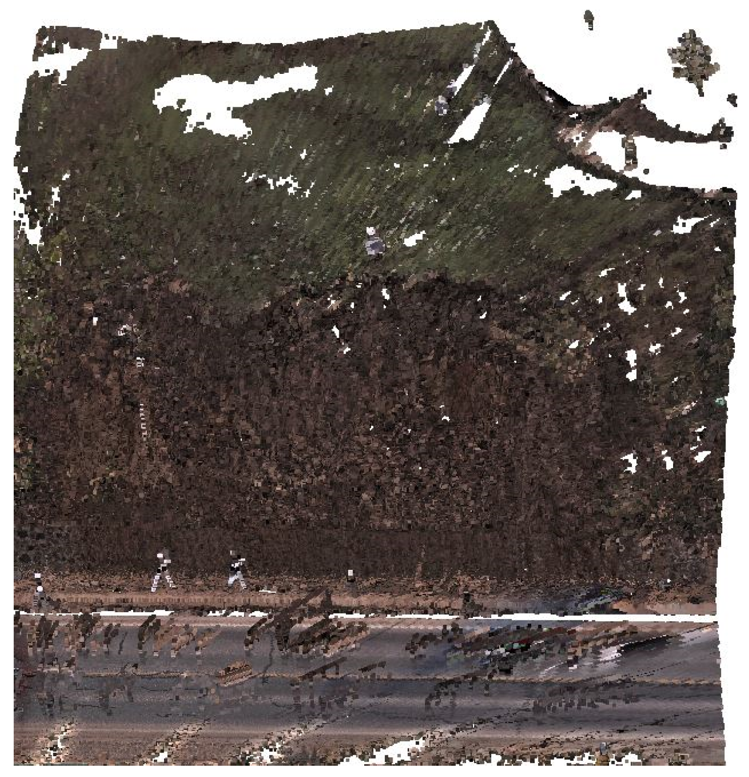
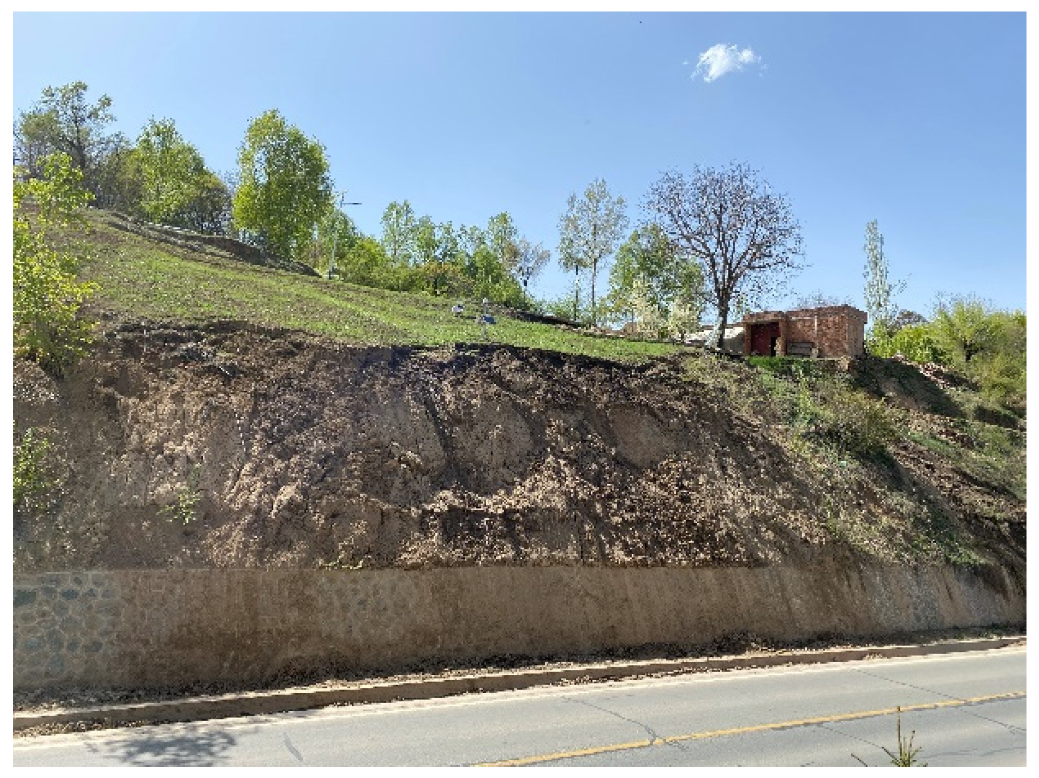
3.2. Actual Experiment
3.2.1. Actual Experiment I
- (I)
- Experiment 1
- (I)
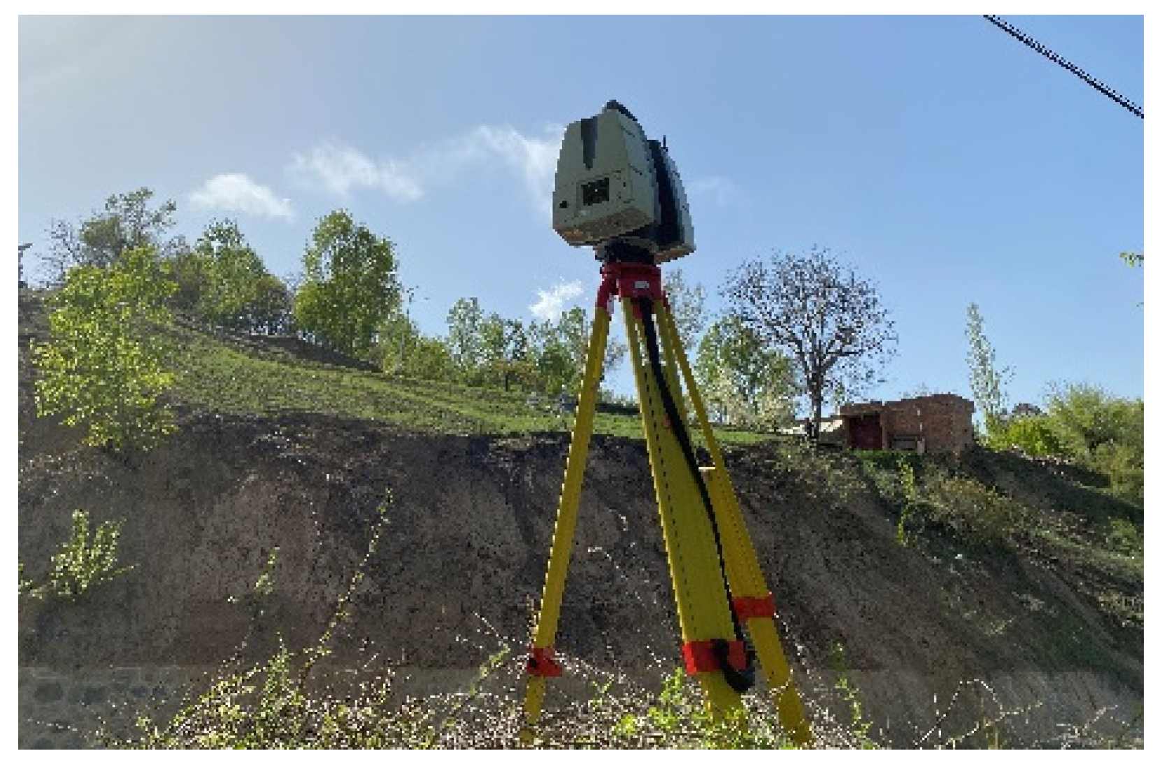
- Triangular pyramid target point cloud acquisition
- (II)
- Data collection based on total station orientation
- (1)
- Leica TS30 total station was used to collect the coordinates of the prism balls near the landslide area.
- (2)
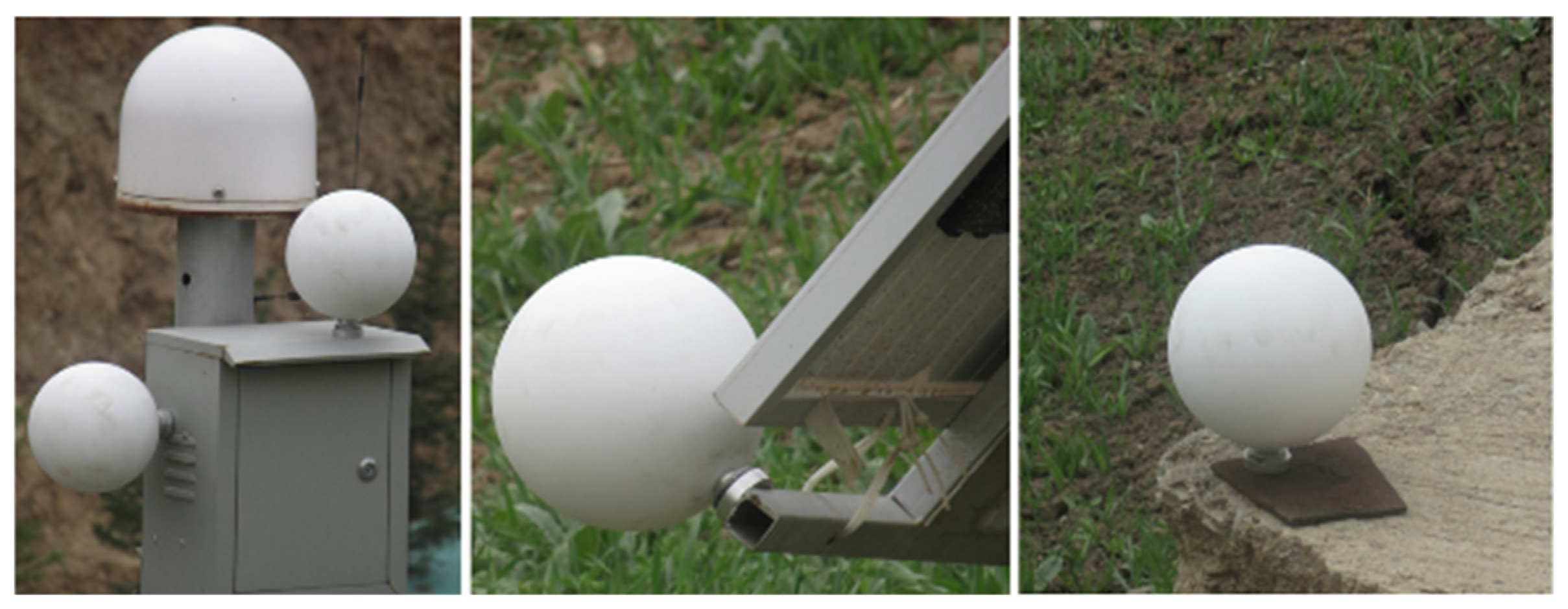
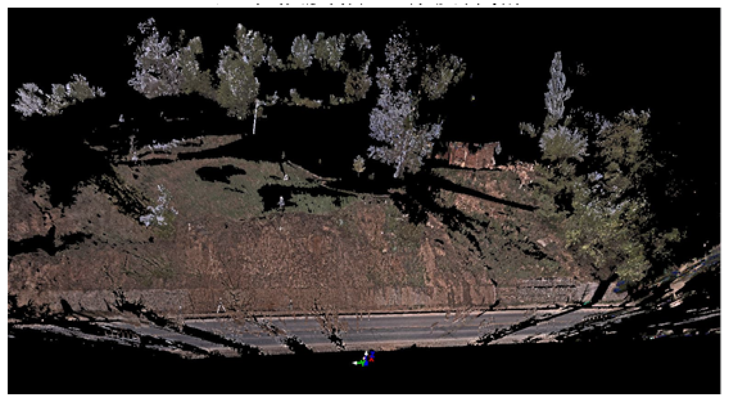
- The coordinates of the prism balls near the landslide area were obtained by fitting point cloud data collected by TLS simultaneously.
- (3)
- The unification of the data.
3.2.2. Actual Experiment II
4. Analysis of Result and Discussion
4.1. The Results of Simulation Experiments
4.1.1. The Result of Simulation Experiment I
4.1.2. The Result of Simulation Experiment II
4.2. The Result of the Actual Experiment
- (I)
- The result of experiment I
4.2.1. The result of PCR Based on Triangular Pyramid Target
4.2.2. The result of PCR Based on Total Station Orientation
- (1)
- In terms of data acquisition, to ensure the accuracy of registration, the data acquisition mode which is based on a fixed triangular pyramid target is simple and is capable of fast operation. It is suitable for good visibility and convenient transportation and is easy to cast in a concrete environment. In addition, based on the total station orientation data acquisition mode, it is not limited by field conditions and has a wide applicability. Especially, in a situation where there are some control points in the stable area, the point cloud can be directly and effectively transformed into the existing coordinate system, which is of great significance to the continuous dynamic monitoring of landslide disasters based on point cloud data.
- (2)
- In terms of PCR, the PCR theory based on a fixed triangular pyramid target and total station orientation is strict. The PCR based on a fixed triangular pyramid target can overcome the problem of low precision in the sphere-based PCR method. The advantage of PCR based on total station orientation is that the point cloud coordinates can be converted to the existing control point coordinate system, which is favorable for the utilization of survey area engineering.
4.2.3. Landslide Based on DTM Difference
- (II)
- The result of experiment II
5. Conclusions
Author Contributions
Funding
Data Availability Statement
Conflicts of Interest
References
- Yao, L.; Sun, H.; Zhu, L.; Zhou, Y. Development and application of deformation monitoring system for lanslide at Funchunjiang Dam. Surv. Rev. 2014, 46, 444–452. [Google Scholar] [CrossRef]
- Gikas, V. 3D Terrestrial laser scanning for geometry documentation and construction management of highway tunnels during excavation. Sensors 2012, 12, 11249–11270. [Google Scholar] [CrossRef] [Green Version]
- Vezocnik, R.; Ambrozic, T.; Sterle, O.; Bilban, G.; Pfeifer, N.; Stopar, B. Use of terrestrial laser scanning technology for long term high precision deformation monitoring. Sensors 2009, 9, 9873–9895. [Google Scholar] [CrossRef] [PubMed]
- He, M.; Zhu, Q.; Du, Z.; Hu, H.; Ding, Y.; Chen, M. A 3D shape descriptor based on contour clusters for damaged roof detection using airborne LiDAR point clouds. Remote Sens. 2016, 8, 189. [Google Scholar] [CrossRef] [Green Version]
- Kasperski, J.; Delacourt, C.; Allemand, P.; Potherat, P.; Jaud, M.; Varrel, E. Application of a terrestrial laser scanner (TLS) to the study of the Séchilienne Landslide (Isère, France). Remote Sens. 2010, 2, 2785–2802. [Google Scholar] [CrossRef] [Green Version]
- Crepaldi, S.; Zhao, Y.; Lavy, M.; Amanzio, G.; Suozzi, E.; De Maio, M. Landslide analysis by multi-temporal terrestrial laser scanning (TLS) data: The Mont de la Saxe landslide. Rend. Online Della Soc. Geol. Ital. 2015, 35, 92–95. [Google Scholar] [CrossRef]
- Wang, D.; Hollaus, M.; Schmaltz, E.; Wieser, M.; Reifeltshammer, D.; Pfeifer, N. Tree stem shapes derived from TLS data as an indicator for shallow landslides. Procedia Earth Planet. Sci. 2016, 16, 185–194. [Google Scholar] [CrossRef] [Green Version]
- Wang, G.; Philips, D.; Joyce, J.; Rivera, F. The integration of TLS and continuous GPS to study landslide deformation: A case study in Puerto Rico. J. Geod. Sci. 2011, 1, 25–34. [Google Scholar] [CrossRef] [Green Version]
- Cina, A.; Piras, M. Performance of low-cost GNSS receiver for landslides monitoring: Test and results. Geomat. Nat. Hazards Risk 2015, 6, 497–514. [Google Scholar] [CrossRef]
- Senkaya, M.; Babacan, A.E.; Karslı, H.; San, B.T. Origins of diverse present displacements in a paleo-landslide area (Isiklar, Trabzon, northeast Turkey). Environ. Earth Sci. 2022, 81, 1–24. [Google Scholar] [CrossRef]
- Stiros, S.C.; Vichas, C.; Skourtis, C. Landslide monitoring based on geodetically derived distance changes. J. Surv. Eng. 2004, 130, 156–162. [Google Scholar] [CrossRef]
- Tzenkov, T.; Gospodinov, S. Geometric analysis of geodetic data for investigation of 3D landslide deformations. Nat. Hazards Rev. 2003, 4, 78–81. [Google Scholar] [CrossRef]
- Klimeš, J.; Rowberry, M.D.; Blahůt, J.; Briestenský, M.; Hartvich, F.; Košťák, B.; Rybář, J.; Stemberk, J.; Štěpančíkováet, P. The monitoring of slow-moving landslides and assessment of stabilisation measures using an optical–mechanical crack gauge. Landslides 2012, 9, 407–415. [Google Scholar] [CrossRef]
- Baroň, I.; Supper, R. Application and reliability of techniques for landslide site investigation, monitoring and early warning–outcomes from a questionnaire study. Nat. Hazards Earth Syst. Sci. 2013, 13, 3157–3168. [Google Scholar] [CrossRef] [Green Version]
- Shi, X.; Hu, X.; Sitar, N.; Kayen, R.; Qi, S.; Jiang, H.; Wang, X.; Zhang, L. Hydrological control shift from river level to rainfall in the reactivated Guobu slope besides the Laxiwa hydropower station in China. Remote Sens. Environ. 2021, 265, 112664. [Google Scholar] [CrossRef]
- Guo, F.; Meng, X.; Qi, T.; Dijkstra, T.; Thorkildsen, J.K.; Yue, D.; Chen, G.; Zhang, Y.; Dou, X.; Shi, P. Rapid onset hazards, fault-controlled landslides and multi-method emergency decision-making. J. Mt. Sci. 2022, 19, 1357–1369. [Google Scholar] [CrossRef]
- Guo, C.; Xu, Q.; Dong, X.; Liu, X.; Yu, J. Geohazard Recognition by Airborne LiDAR Technology in Complex Mountain Areas. Geomat. Inf. Sci. Wuhan Univ. 2021, 46, 1538–1547. [Google Scholar]
- Abellán, A.; Vilaplana, J.; Calvet, J.; García-Sellés, D.; Asensio, E. Rockfall monitoring by terrestrial laser scanning-case study of the basaltic rock face at Castellfollit de la Roca (Catalonia, Spain). Nat. Hazards Earth Syst. Sci. 2011, 11, 829–841. [Google Scholar] [CrossRef] [Green Version]
- Kayen, R.; Pack, R.; Bay, J.; Collins, B. Ground-Lidar visualization of surface and structural deformatios of the Niigata Ken Chuetsu. Earthq. Spectra 2006, S1, 147–162. [Google Scholar] [CrossRef]
- Liu, W.; Xie, M. Landslide monitoring based on point cloud density characteristics. Rock Soil Mech. 2020, 41, 3748–3756. [Google Scholar]
- Zhao, J.; Du, S.; Liu, Y.; Saif, B.S.; Hou, Y.; Guo, Y.C. Evaluation of the stability of the palatal rugae using the three-dimensional superimposition technique following orthodontic treatment. J. Dent. 2022, 119, 104055. [Google Scholar] [CrossRef] [PubMed]
- Yang, M.; Gan, S.; Yuan, X.; Gao, S.; Zhu, Z.; Yu, H. Study on data acquisition and registration experiment of terretrial laser scanning point clouds under complicated banded terrain condition. Bull. Surv. Mapp. 2018, 5, 35–40. [Google Scholar]
- Zeybek, M.; Şanlıoğlu, İ. Accurate determination of the Taşkent (Konya, Turkey) landslide using a long-range terrestrial laser scanner. Bull. Eng. Geol. Environ. 2015, 74, 61–76. [Google Scholar] [CrossRef]
- Hsieh, Y.C.; Chan, Y.C.; Hu, J.C.; Chen, Y.Z.; Chen, R.F.; Chen, M.M. Direct measurements of bedrock incision rates on the surface of a large dip-slope landslide by multi-period airborne laser scanning DEMs. Remote Sens. 2016, 8, 900. [Google Scholar] [CrossRef] [Green Version]
- Xian, Y.; Xiao, J.; Wang, Y. A fast registration algorithm of rock point cloud based on spherical projection and feature extraction. Front. Comput. Sci. 2019, 13, 170–182. [Google Scholar] [CrossRef]
- Kümmerle, J.; Kühner, T.; Lauer, M. Automatic calibration of multiple cameras and depth sensors with a spherical target. In Proceedings of the 2018 IEEE/RSJ International Conference on Intelligent Robots and Systems (IROS), Madrid, Spain, 1–5 October 2018; pp. 1–8. [Google Scholar]
- Zhou, Y.; Han, D.; Hu, K.; Qin, G.; Xiang, Z.; Ying, C.; Zhao, L.; Hu, X. Accurate virtual trial assembly method of prefabricated steel components using terrestrial laser scanning. Adv. Civ. Eng. 2021, 2021, 9916859. [Google Scholar] [CrossRef]
- Li, J.; Hu, Q.; Ai, M. Point cloud registration based on one-point ransac and scale-annealing biweight estimation. IEEE Trans. Geosci. Remote Sens. 2021, 59, 9716–9729. [Google Scholar] [CrossRef]
- Chen, Z.; Zhang, B.; Han, Y.; Zuo, Z.; Zhang, X. Modeling accumulated volume of landslides using remote sensing and DTM data. Remote Sens. 2014, 6, 1514–1537. [Google Scholar] [CrossRef] [Green Version]
- Artese, S.; Perrelli, M. Monitoring a landslide with high accuracy by total station: A DTM-based model to correct for the atmospheric effects. Geosciences 2018, 8, 46. [Google Scholar] [CrossRef] [Green Version]
- Pawluszek, K.; Borkowski, A.; Tarolli, P. Sensitivity analysis of automatic landslide mapping: Numerical experiments towards the best solution. Landslides 2018, 15, 1851–1865. [Google Scholar] [CrossRef] [Green Version]
- Xu, P.; Shimada, S. Least squares parameter estimation in multiplicative noise models. Commun. Stat. Simul. Comput. 2000, 29, 83–96. [Google Scholar] [CrossRef]
- Shi, Y.; Xu, P.; Peng, J.; Shi, C.; Liu, J. Adjustment of measurements with multiplicative errors: Error analysis, estimates of the variance of unit weight, and effect on volume estimation from LiDAR-type digital elevation models. Sensors 2014, 14, 1249–1266. [Google Scholar] [CrossRef] [PubMed] [Green Version]
- Wang, L.; Yu, D. Virtual observation method to ill-posed total least squares problem. Acta Geod. Cartogr. Sin. 2014, 43, 575–581. [Google Scholar]
- Xu, P. Truncated SVD methods for discrete linear ill-posed problems. Geophys. J. Int. 1998, 135, 505–514. [Google Scholar] [CrossRef]
- Koch, K.R.; Kusche, J. Regularization of geopotential determination from satellite data by variance components. J. Geod. 2002, 76, 259–268. [Google Scholar] [CrossRef]
- Hoerl, A.E.; Kennard, R.W. Ridge regression: Biased estimation for nonorthogonal problems. Technometrics 1970, 12, 55–67. [Google Scholar] [CrossRef]
- Wang, L.; Chen, T. Virtual Observation Iteration Solution and A-Optimal Design Method for Ill-Posed Mixed Additive and Multiplicative Random Error Model in Geodetic Measurement. J. Surv. Eng. 2021, 147, 04021016. [Google Scholar] [CrossRef]
- Du, S.; Zheng, N.; Ying, S.; Liu, J. Affine iterative closest point algorithm for point set registration. Pattern Recognit. Lett. 2010, 31, 791–799. [Google Scholar] [CrossRef]
- Li, P.; Wang, R.; Wang, Y.; Tao, W. Evaluation of the ICP algorithm in 3D point cloud registration. IEEE Access 2020, 8, 68030–68048. [Google Scholar] [CrossRef]
- Pomerleau, F.; Colas, F.; Siegwart, R.; Magnenat, S. Comparing ICP variants on real-world data sets. Auton. Robot. 2013, 34, 133–148. [Google Scholar] [CrossRef]
- Deakin, R.E. A note on the Bursa-Wolf and Molodensky-Badekas Transformations; School of Mathematical and Geospatial Sciences, RMIT University: Melbourne, VIC, Australia, 2006; pp. 1–21. [Google Scholar]
- Golub, G.H.; Van Loan, C.F. An analysis of the total least squares problem. SIAM J. Numer. Anal. 1980, 17, 883–893. [Google Scholar] [CrossRef]
- Oktaba, W. Tests of Hypotheses for the General Gauss-Markov Model. Biom. J. 1984, 26, 415–424. [Google Scholar] [CrossRef]
- Jeng, F.C.; Woods, J.W. Compound Gauss-Markov random fields for image estimation. IEEE Trans. Signal Processing 1991, 39, 683–697. [Google Scholar] [CrossRef]
- Shi, Y.; Xu, P. Adjustment of measurements with multiplicative random errors and trends. IEEE Geosci. Remote Sens. Lett. 2020, 18, 1916–1920. [Google Scholar] [CrossRef]
- Davidon, W.C. New least-square algorithms. J. Optim. Theory Appl. 1976, 18, 187–197. [Google Scholar] [CrossRef]
- Heyde, C.C. Quasi-Likelihood and Its Application: A General Approach to Optimal Parameter Estimation; Springer: New York, NY, USA, 1997; pp. 32–69. [Google Scholar]
- Gregor, J.; Fessler, J.A. Comparison of SIRT and SQS for regularized weighted least squares image reconstruction. IEEE Trans. Comput. Imaging 2015, 1, 44–55. [Google Scholar] [CrossRef] [Green Version]
- Hansen, P.C. Analysis of discrete ill-posed problems by means of the L-curve. SIAM Rev. 1992, 34, 561–580. [Google Scholar] [CrossRef]
- Vogel, C.R. Non-convergence of the L-curve regularization parameter selection method. Inverse Probl. 1996, 12, 535. [Google Scholar] [CrossRef] [Green Version]
- Wang, L.; Chen, T.; Zou, C. Weighted least squares regularization iteration solution and precision estimation for ill-posed multiplicative error mode. Acta Geod. Cartogr. Sin. 2021, 50, 589–599. [Google Scholar]
- Xu, P.; Shi, Y.; Peng, J.; Liu, J.; Shi, C. Adjustment of geodetic measurements with mixed multiplicative and additive random errors. J. Geod. 2013, 87, 629–643. [Google Scholar] [CrossRef]
- Shi, Y.; Xu, P. Comparing the estimates of the variance of unit weight in multiplicative error models. Acta Geod. Geophys. 2015, 50, 353–363. [Google Scholar] [CrossRef] [Green Version]
- Hill, C.A.; Harris, M.; Ridley, K.D.; Jakeman, E.; Lutzmann, P. Lidar frequency modulation vibrometry in the presence of speckle. Appl. Opt. 2003, 42, 1091–1100. [Google Scholar] [CrossRef] [PubMed]
- Leigh, C.L.; Kidner, D.B.; Thomas, M.C. The use of LiDAR in digital surface modelling: Issues and errors. Trans. GIS. 2009, 13, 345–361. [Google Scholar] [CrossRef]
- Hladik, C.; Alber, M. Accuracy assessment and correction of a LIDAR-derived salt marsh digital elevation model. Remote Sens. Env. 2012, 121, 224–235. [Google Scholar] [CrossRef]
- Jia, C.; Jin, Z.; Yang, P.; Tang, Z. Stability analysis on landslide in section K181 + 840 ~ K182 + 040 of Lin − Da Highway. J. Lanzhou Petrochem. Polytech. 2018, 18, 26–28. [Google Scholar]
- Jia, X.; Yin, X.; Ren, Y.; Fu, Z. Climate change of Linxia of Gansu Province in recent 43 years. J. Arid Meteorol. 2012, 30, 249–254. [Google Scholar]
- Leica ScanStation P50—Long Range 3D Terrestrial Laser Scanner. Available online: https://leica-geosystems.com/products/laser-scanners/scanners/leica-scanstation-p50 (accessed on 3 June 2022).
- Leica TS30 Champion’s League. Available online: https://www.bandwork.my/product/pdf/731201461738PMTS30_Brochure_en.pdf (accessed on 3 June 2022).
- Kobler, A.; Pfeifer, N.; Ogrinc, P.; Todorovski, L.; Oštir, K.; Džeroski, S. Repetitive interpolation: A robust algorithm for DTM generation from Aerial Laser Scanner Data in forested terrain. Remote Sens. Environ. 2007, 108, 9–23. [Google Scholar] [CrossRef]


| Point Number | y | Point Number | y |
|---|---|---|---|
| 1 | 8.8529 | 17 | 52.9943 |
| 2 | 9.3072 | 18 | 66.6330 |
| 3 | 10.0079 | 19 | 80.6002 |
| 4 | 8.0547 | 20 | 80.1413 |
| 5 | 13.7458 | 21 | 106.8200 |
| 6 | 13.1323 | 22 | 112.3601 |
| 7 | 12.5329 | 23 | 136.7752 |
| 8 | 16.5769 | 24 | 184.5394 |
| 9 | 13.1390 | 25 | 254.6235 |
| 10 | 17.2795 | 26 | 242.7289 |
| 11 | 19.0292 | 27 | 323.5583 |
| 12 | 22.8096 | 28 | 360.2978 |
| 13 | 26.2168 | 29 | 482.2399 |
| 14 | 27.0681 | 30 | 453.0284 |
| 15 | 34.8363 | 31 | 595.4323 |
| 16 | 40.9079 |
| Parameter | Value |
|---|---|
| Scan range mode | from 0.4 to120 m from 0.4 to 270 m from 0.4 to 570 m, >1 km |
| Scan Rate | up to 1,000,000 points per second |
| Vertical/horizontal field-of-view | 360°/290° |
| Range noise * | 0.4 mm rms at 10 m 0.5 mm rms at 50 m |
| Operating temperature | −4° F to + 122° F |
| Dual-axis compensator | accuracy 1.5″ |
| Parameter | Value | |
|---|---|---|
| Accuracy of angle | Horizontal and Vertical | 0.5″ |
| Distance Measurement Range | Round Prism (GPR1) | 3500 m |
| Accuracy of distance | Standard (prism) | 1 mm + 1 ppm |
| Control Point | x/m | y/m | z/m |
|---|---|---|---|
| SCP1 | 531.375 | 533.190 | 761.551 |
| SCP2 | 535.557 | 522.346 | 762.020 |
| SCP3 | 479.548 | 473.771 | 766.402 |
| SCP4 | 412.943 | 401.501 | 772.336 |
| Method | ||||||||
|---|---|---|---|---|---|---|---|---|
| True value | 10 | 4 | 2 | 1 | 0.5 | 2 | 0.3 | — |
| LS | 19.64 | −147.21 | 442.38 | −453.75 | 189.92 | −25.37 | 12.0984 | 678.47 |
| bcLS | 11.45 | −2.19 | 6.27 | 7.96 | −8.11 | 3.99 | 20.98 | 13.61 |
| RWLS | 10.77 | 2.12 | 1.46 | 2.52 | −1.46 | 2.46 | 1.26 | 3.28 |
| Method | ||||||
|---|---|---|---|---|---|---|
| true value | −3.5 | 15 | 8 | −3 | 0.3 | — |
| LS | 21.68 | 21.00 | −11.25 | −14.87 | 4.52 | 34.38 |
| bcWLS | −6.44 | 18.99 | 8.59 | −1.69 | 4.36 | 3.18 |
| RWLS | −1.94 | 14.91 | 7.46 | −3.91 | 0.42 | 1.88 |
| Point Number | x/m | y/m | z/m |
|---|---|---|---|
| CP1 | 5.989 | 22.562 | −4.090 |
| CP2 | 12.648 | 15.101 | −4.803 |
| CP3 | 32.494 | −6.676 | −6.480 |
| Point Number | x/m | y/m | z/m |
|---|---|---|---|
| CP1 | −12.412 | 19.621 | −4.134 |
| CP2 | −2.413 | 19.380 | −4.847 |
| CP3 | 27.049 | 18.977 | −6.523 |
| Method | |||||||
|---|---|---|---|---|---|---|---|
| LS | −0.368 | 0.340 | 0.128 | −0.007 | −0.015 | 0.0003 | 13.12 |
| bcWLS | −0.265 | 0.135 | 0.313 | −0.023 | −0.062 | 0.0005 | 6.93 |
| RWLS | −0.165 | 0.102 | 0.033 | 0.016 | −0.002 | 0.0267 | 2.34 |
| Method | |||||||
|---|---|---|---|---|---|---|---|
| LS | −0.532 | 1.234 | 0.568 | −0.146 | −0.051 | 0.021 | 26.16 |
| bcWLS | −0.389 | 0.657 | 0.425 | −0.072 | −0.081 | 0.0063 | 8.24 |
| RWLS | −0.132 | 0.231 | 0.046 | 0.024 | −0.006 | 0.001 | 2.34 |
Publisher’s Note: MDPI stays neutral with regard to jurisdictional claims in published maps and institutional affiliations. |
© 2022 by the authors. Licensee MDPI, Basel, Switzerland. This article is an open access article distributed under the terms and conditions of the Creative Commons Attribution (CC BY) license (https://creativecommons.org/licenses/by/4.0/).
Share and Cite
Zhao, L.; Ma, X.; Xiang, Z.; Zhang, S.; Hu, C.; Zhou, Y.; Chen, G. Landslide Deformation Extraction from Terrestrial Laser Scanning Data with Weighted Least Squares Regularization Iteration Solution. Remote Sens. 2022, 14, 2897. https://doi.org/10.3390/rs14122897
Zhao L, Ma X, Xiang Z, Zhang S, Hu C, Zhou Y, Chen G. Landslide Deformation Extraction from Terrestrial Laser Scanning Data with Weighted Least Squares Regularization Iteration Solution. Remote Sensing. 2022; 14(12):2897. https://doi.org/10.3390/rs14122897
Chicago/Turabian StyleZhao, Lidu, Xiaping Ma, Zhongfu Xiang, Shuangcheng Zhang, Chuan Hu, Yin Zhou, and Guicheng Chen. 2022. "Landslide Deformation Extraction from Terrestrial Laser Scanning Data with Weighted Least Squares Regularization Iteration Solution" Remote Sensing 14, no. 12: 2897. https://doi.org/10.3390/rs14122897