Article

Using Support Vector Machine (SVM) with GPS Ionospheric TEC Estimations to Potentially Predict Earthquake Events

1
Department of Computer Sciences, Ariel University, Ariel 40700, Israel
2
Department of Civil Engineering, Ariel University, Ariel 40700, Israel
3
Department of Physics, Ariel University, Ariel 40700, Israel
4
Department of Geophysics, Eastern R&D Center, Ariel 40700, Israel
5
Astrophysics Geophysics and Space Science Research Center, Ariel University, Ariel 40700, Israel
6
School of Sustainability, Reichman University, IDC, Herzliya 4610101, Israel
*
Author to whom correspondence should be addressed.
Remote Sens. 2022, 14(12), 2822; https://doi.org/10.3390/rs14122822
Submission received: 9 May 2022 / Revised: 9 June 2022 / Accepted: 9 June 2022 / Published: 12 June 2022

Abstract

:
There are significant controversies surrounding the detection of precursors that may precede earthquakes. Natural hazard signatures associated with strong earthquakes can appear in the lithosphere, troposphere, and ionosphere, where current remote sensing technologies have become valuable tools for detecting and measuring early warning signals of stress build-up deep in the Earth’s crust (presumably associated with earthquake events). Here, we propose implementing a machine learning support vector machine (SVM) technique, applied with GPS ionospheric total electron content (TEC) pre-processed time series estimations, to evaluate potential precursors caused by earthquakes and manifested as disturbances in the TEC data. After filtering and screening our data for solar or geomagnetic influences at different time scales, our results indicate that for large earthquakes (>Mw 6), true negative predictions can be achieved with 85.7% accuracy, and true positive predictions with an accuracy of 80%. We tested our method with different skill scores, such as accuracy (0.83), precision (0.85), recall (0.8), the Heidke skill score (0.66), and true skill statistics (0.66).

Graphical Abstract

1. Introduction

1.1. Natural Hazard Signatures Associated with Geodynamic Processes

Natural hazards (e.g., earthquakes) have significantly threatened humans throughout history [1,2]. Remote sensing technologies operating at wide frequency ranges, using either sound or electromagnetic emitted waves, have become valuable tools for detecting and measuring signatures presumably associated with such events [3,4]. In the last three decades, predicting when and where natural hazards were to occur has been challenging in geoscience-related research [5,6]. The occurrences of earthquakes are correlated with the dynamics of the earth’s crust [7,8], consisting of semi-rigid tectonic plates of various sizes [9]. When these plates collides, they can cause one edge of the plate to slide under the other [10,11], resulting in stress accumulation within the earth’s crust [12]. This leads to mechanical deformations, and results in the rupture of the crust when the deformation exceeds the limit of the mechanical forces [12]. Since most of the governing forces and basic mechanics of earthquake events cannot be cast into physical and numerical models, and since we lack sufficiently detailed and real-time measurements, accurate forecasting of such events is not currently possible [3,13,14,15].
On the other hand, observational and modeling results have confirmed the existence and detectability of earthquake and tsunami signatures in the ionosphere caused by both acoustic and gravity waves, disturbing the electron density in the F-region [16,17,18,19,20,21].
Regarding the connection between the F-region and earthquakes—the source of the earthquake generates acoustic and gravity-acoustic waves that propagate laterally and upward, away from the source and through the ionospheric layers. This means that such hazards can create atmospheric and ionospheric perturbations via direct coupling [19]. Such signatures have also been confirmed by anomalous increases in the intensity of the electromagnetic signal, received in the VLF/ULF bands, during the period immediately preceding an earthquake [22,23,24], and are caused by ionospheric D-layer electron density disturbances. However, there are still a fair amount of ambiguities regarding the scientific validations of these discoveries as reliable tools that may be used for detecting precursor natural-hazard-generated ionospheric perturbations. For example, after the devastating Tōhoku-oki earthquake (Mw 9.1) and tsunami that took place in Japan on 11 March 2011, using Japan’s dense GPS satellite network, Heki [14] reported that a clear precursor was detected in the form of a positive anomaly of ionospheric total electron content (TEC). This began about 40 min before the earthquake and reached nearly 10% of the background TEC, and lasted until atmospheric waves arrived at the ionosphere. Kuo et al. [20,21] suggested that these ionospheric density variations could be caused by Earth surface charges (or currents) produced from electric currents associated with the stressed rock. However, when Komjathy et al. [25] investigated the global ionospheric TEC perturbations just before and after the event, they concluded that the geomagnetic activity indicated storm conditions that were already apparent from processed GEONET data one day prior to and after the event. The same ambiguity can be found with ionospheric D-layer electron density disturbances extracted from VLF measurements. Hayakawa et al. [22] reported on a possible VLF sub-ionospheric precursor for the same earthquake in Japan. They found a remarkable anomaly for the NLK-Chofu great circle path on 5 and 6 March in the form of nighttime average amplitude signal decrees that exceeded 4 σ . The anomaly was found on the same day along other propagation paths (from NLK to both Kasugai and Kochi), although it was less enhanced. Later on, Cohen and Marshall [23] reported that after examining VLF data recorded at a site in Onagawa, Japan, located approximately 102 km from the epicenter, no radio emissions preceding or coincident to the onset of the earthquake were found. An examination of VLF data from narrowband transmitters also showed no anomalous activity in the days or weeks preceding the earthquake.

1.2. Machine Learning and Deep Learning

State-of-the-art forecasting systems today are mostly based on numerical models, and these are unable to accurately describe the physical processes leading to earthquake events. The physics and complexities of fault motion in different tectonic environments include many characteristics related to the structure of the Earth’s crust, from plate tectonics to the microscopic processes involving friction, electric charge generation, and various chemical reactions [7,24]. Thus, the lack of sufficiently detailed real-time measurements prevents accurate forecasting of earthquake events. Recent advances in cloud-based big-data technologies now make data-driven solutions feasible for increasing the numbers of scientific computing applications [26,27]. One data-driven solution is machine learning (ML), which brings patterns in large data sets to the surface by finding complex mathematical relationships within the data [28]. Thus, researchers are gradually harnessing multivariate data analysis techniques from ML disciplines to predict occurrences of natural hazard events from past distribution patterns [6,29]. Algorithms that are commonly used to tackle classification and regression problems include linear regression [30], decision trees and random forest (RF) [31], and support vector machines (SVMs) [32]. Additionally, there are deep learning (DL) models that are based on artificial neural networks (ANNs), inspired by the biological neural network of the brain [33]. The state-of-the-art DL neural network architectures include convolutional neural networks (CNNs), recurrent neural networks (RNNs), and LSTM (long short-term memory).

1.3. Ionospheric Total Electron Content (TEC)

The ionosphere is a region of Earth’s upper atmosphere, extending (approximately) between 60 and 1000 km, where high energy extreme ultra-violet (EUV) and X-ray solar radiation ionizes the atmospheric atoms and molecules, forming a layer of free electrons [26,34]. Other phenomena, such as solar flare, geomagnetic storms, energetic charged particles, and cosmic rays also have an ionizing effect and can contribute to the ionospheric total electron density concentration [27,28,35,36,37,38]. The ionosphere structure and electron peak density changes significantly with altitude, latitude, longitude, universal time, season, solar cycle, and certain solar and geomagnetic activity, making it dynamically variable, thus causing it to be a key source of errors for technologies, such as the global navigation satellite system (GNSS) and interferometric synthetic aperture radar (InSAR) [28,35,36,37,38]. Spectral variability of solar radiation along with density gradients of several elements in the atmosphere create regions within the ionosphere, called the D, E, and F-layers [39]. The F2 layer, extended between about 250 and 800 km [40], has the highest concentration of free electron and ions in the atmosphere and is considered the most dynamic plasma layer in the ionosphere [41].
GNSS technology is a unique tool for continuous monitoring of the ionosphere state on a global scale [26]. It enables the estimation of the total electron content (TEC) of the global ionosphere/plasmasphere stretching up to a height of about 20,000 km [42]. GNSS is based on the accurate assessment of the travel time of the radio signals transmitted from satellites high above the earth’s surface [36]. As these radio signals propagate through the earth’s atmospheric layers (mainly along the troposphere and ionosphere) they are significantly affected by the physical characteristics of these layers and, thus, the propagation speed is reduced [43]. The extent of the delay depends largely on the temperature, pressure, and water vapor distribution, which differ considerably in space and time [44,45,46,47,48,49]. In contrast to the nondispersive tropospheric interaction, the speed at which radio signals propagate at a particular height through the ionosphere is constrained by the free electron density concentration in surrounding areas [50], and the radio signal phase speed is essentially increased by the existence of free electrons. As a result, the radio signal phase accelerates as it travels through the layer, which is manifested as an early arrival at the receiver antenna compared with a complete vacuum propagation time [51]. This early arrival is commonly defined as a phase advance. The total vertical ionospheric range error within a traveling radio signal is assessed by integrating the free electron density concentration through the entire path from the satellite to the ground receiver and, consequently, is proportional to the TEC in the ionosphere [38], where one TEC Unit (TECU) is defined as the total number of free electrons in a cylinder with a base area of 1 m 2 , which is equal to 10 16 electrons m 2 . The outline of the paper is as follows. Section 2 presents the motivation for using a machine learning technique with GPS ionospheric TEC data and gives a potential explanation for TEC enhancement as a possible earthquake precursor. Section 3 describes the datasets and methodology we used in this study. Section 4 presents the SVM model performance using different skill scores. The discussion and conclusions follow in Section 5 and Section 6, respectively.

2. Motivation

Among the precursory phenomena associated with earthquake predictions, the ionospheric TEC enhancement preceding earthquake events has attracted significant scientific attention. Regarding stress—rocks activate positive holes as charges that carry and generate electric currents [52]. Positive hole charge carriers accumulate at the Earth’s surface and charged O 2 + ions from field-ionization accumulate in the air near the region of stressed rocks [53]. As rocks are subjected to stress, they activate hole charge carriers. Except for pure white marble, every igneous and high-grade metamorphic rock tested has produced hole charge carriers when stressed [54]. The positively-charged carriers can spread through less stressed (and even nominally unstressed) rocks. The unstressed rocks become positively charged and the stressed rocks negatively charged due to the loss of the charge carriers in the stressed region. Regarding oceanic regions–the 2011 Tōhoku-oki earthquake charge carrier location had higher mobility than on land because of the higher conductivity of water [55]. The accumulated surface charge over land or ocean drives the current outward. After the charge neutralization time, it is possible that some surface charges are transported into the ionosphere. The ultimate effect is the current flowing into the ionosphere. The direction of the dynamo current flowing in the atmosphere depends on the sign of the generated charges over the Earth’s surface near the stressed rock region: downward to negative surface charge regions, and upward from positive ones.

3. Datasets and Methodology

The datasets that were used in this study, as well as the methodology, data pre-processing, and machine learning model are as follows:

3.1. Datasets

Our main goal was to gain new insight into the possibility of predicting earthquake occurrences using TEC value anomalies. To eliminate all non-related geodynamic effects (e.g., solar flares, coronal mass ejections, geomagnetic storms, and X-ray flux events), we excluded all earthquake events that took place during enhanced solar activity (X or M class solar flares and large scale coronal mass ejections).

3.1.1. Earthquakes Dataset

For the earthquakes dataset, we used the US Geological Survey (USGS) (https://earthquake.usgs.gov/, accessed on 20 June 2020) dataset, which provides the most rapid and accurate information regarding the location, size, and depth for all recorded earthquake events worldwide (Figure 1). The dataset also provides an extensive seismic data since 1850. Since we aimed to study how ML methods can be implemented with GPS ionospheric TEC estimations to predict earthquakes, we only examined the earthquakes that could be correlated with available GPS ionospheric TEC data between the years 1998 and 2021 (i.e., TEC data for the day of the earthquake and 48 consecutive hours before). Additionally, we only examined earthquake events where the number of sunspots on the day of the earthquake was at most 50, with no solar flare recorded on that day. After sorting through the entire database, we ended up with 106 earthquakes with magnitudes larger than Mw 6; thus, we applied our methodology and analysis only to the high magnitude earthquakes (i.e., larger than Mw 6).

3.1.2. TEC Dataset

For the TEC dataset, we used the International GNSS Service (IGS) Analysis Centre dataset, which contains final global ionospheric TEC maps, extracted from averaging four different available models (CODE-University of Bern in Switzerland, ESA-ESOC Darmstadt Germany, JPL-Jet Propulsion Lab in Pasadena USA, and UPC-University Polytechnic Catalonia in Barcelona, Spain) [6]. The IGS dataset also includes rapid global TEC maps in the cylindrical projection along with root mean square error (RMSE) values and rapid TEC maps in polar projection (https://spdf.gsfc.nasa.gov/pub/data/gps/tec15min_igs/, accessed on 10 January 2020). The TEC maps (Figure 2) are produced with a resolution of 15 min, 5 and 2 . 5 , in time, longitude, and latitude, respectively. This results in 96 maps per day with dimensions of 73 × 71 for each map.

3.1.3. Solar Flares, Geomagnetic Storms, and Coronal Mass Ejection (CME) Datasets

For the solar flare and geomagnetic datasets, we used NOAA SWPC data (spaceweatherlive.com, accessed on 20 June 2020), which provide real-time and archived auroral and solar activity data (since June 1996), based on the space environment monitor instrument subsystem, carried on board Geostationary Operational Environmental Satellites (GOES). The dataset consists of the strongest 50 solar flares each year; for each flare, the exact level, region, and time of the occurrence are provided. We had 1250 solar flares in the dataset (regarding the years in the range of the earthquake dataset).
For the geomagnetic activity, we used NOAA SWPC data (https://www.swpc.noaa.gov/products/planetary-k-index, accessed on 20 June 2020), which provide Kp index values, are considered excellent proxies of disturbances in the Earth’s magnetic field, and are used by SWPC to determine whether geomagnetic warnings are issued. As such, we filtered out all of the relevant maps during days with high Kp index values ( k p 6 ). For the CME dataset, we used the SOHO LASCO CME catalogue (https://cdaw.gsfc.nasa.gov/CME_list/, accessed on 20 June 2020), which contains all CMEs manually identified since 1996 from the Large Angle and Spectrometric Coronagraph (LASCO) on board the Solar and Heliospheric Observatory (SOHO) mission.

3.2. Methodology

The overall methodology we used in this approach is as follows. As a first step, we applied a TEC data elimination procedure, followed by pre-processing and data splitting. Finally, we applied SVM with pre-processed ionospheric VTEC data to attempt to predict earthquakes.

3.2.1. TEC Data Rejection

As we aimed to produce a reliable prediction of earthquake occurrence, we excluded all GPS ionospheric maps during days where there were solar disturbances and strong solar flare activity, due to the influence of extreme UV and X-ray radiation on the ionospheric F2 layer [6]. Moreover, we ensured that no strong CME events took place during the 48 h prior to all earthquake events used in our study (the CMEs that took place were defined as very poor events).
By doing so, we were left with a model that predicted earthquakes based on ionospheric enhancements originating from non-solar and geomagnetic sources influencing the ionospheric TEC density.

3.2.2. TEC Data Pre-Processing

1.
Epicenter TEC value evaluation:
As mentioned above, the TEC maps were produced with spatial resolutions of 5 and 2 . 5 in longitude and latitude, respectively, at a 15 min temporal resolution. We were interested in examining the ionospheric TEC changes above the earthquake epicenters, up to 48 h before each event, but not all corresponded epicenter TEC maps are available between 1998 and 2021. In this step, we calculated for each earthquake epicenter the corresponded ionospheric TEC value (Figure 3) by taking the weighted average value of the closest available points in the map using the equation:
V a l u e = i = 1 s i z e ( V ) ( W i · V i ) w W w
where W i is the weight of the i t h neighbour, which is defined as its inverse distance from the epicenter, and V i is its value.
2.
Epicenter time series generation:
In the next step, we generated (for each earthquake epicenter) a TEC time series of 48 h before the recorded main shock, again using the algorithm described immediately above. As each hour consists of four measurements, our final vector has 192 TEC values.
3.
TEC detrending time series:
After obtaining the epicenter time series, we filtered the solar activity diurnal trend (as can be seen in Figure 4), by subtracting a smoothed moving average time window size, equal to 1 h of data, from the original time series data (Figure 5) using the following formula:
x i ^ = x i 1 4 j = i 4 i + 4 x j
where x ^ is the detrended signal, and x is the original signal.
4.
Ionospheric Quiet days–mean and standard deviation TEC time series estimation:
Finally, we estimated the ionospheric TEC quiet days, where a quiet day corresponding to an earthquake event is defined as the same day and time of a different year, where there were no earthquakes or solar disturbances (solar storms, geomagnetic storms, or CMEs) events, with respect to the monthly mean SSN number during the event. For example, the 2011 Tōhoku earthquake occurred in March, where the monthly mean SSN number was 78, i.e., higher than 50 (which is our fixed threshold for determining low or high solar cycle activities); thus, a corresponding quite day for this event was chosen from the same day and time of a different year, where there were no earthquakes or solar disturbances, and the monthly mean SSN number exceeded 50 SSN.
Figure 6 shows an example of the TEC time series data around 11 March from 1999–2020. Using our quiet days definition described above, we found 15 candidate days, where the monthly mean SSN number exceeded 50 SSN, and from which we randomly picked one for each training set. Figure 7 shows an example of a randomly picked normalized quiet day (March 2013) compared with the 11 March 2011 Tōhoku earthquake day, which was also normalized by subtracting the minimum TEC time series value from the original time series and then dividing it by its maximum value.
Additional case studies for other large earthquake events compared with the corresponding randomly picked normalized quiet days are shown in Appendix A.

3.2.3. Bayesian Hyperparameter Optimization for SVM

Support vector machine (SVM) is a supervised machine learning approach that is based on the kernel method, which is often used for classification and regression missions [56,57,58,59]. As we aimed to predict whether an earthquake event was about to occur or not, we used the SVM to classify ionospheric TEC enhancements prior to earthquake events during low and high solar cycle activities, where we introduced the pre-earthquake TEC time series sample as a positive instance of an earthquake event, and its corresponding quiet day time series as a negative instance (i.e., an earthquake would not occur). As such, we sought to optimize the SVM hyperparameters in order to find the kernel function and parameters yielding the most accurate model. To do this, we employed MATLAB’s ‘fitcsvm’ function, which automatically compares different kernels, such as the radial basis function and polynomials of different degrees, and also tunes the kernel hyperparameters, such as the penalties for false negatives, and false positives, and the inner trade-off between smaller sample errors and larger margins. The optimization process searches for the optimal hyperparameters using the Bayesian method [60], which initializes a random point in the hyperparameter space and then iteratively evaluates promising hyperparameter configuration based on the current model; if these new parameters yield improvements, the current model is updated with the new hyperparameters [61]. Bayesian optimization aims to gather observations revealing as much information as possible about the function and the location of its optimum [62].
We found that the optimal result was obtained by a polynomial kernel function of degree 2.

4. Experimental Results

In this section, we show our model performance results using known skill score metrics composed of different combinations between true positive (TP), false negative (FN), true negative (TN) and false positive (FP) ratios. The confusion matrix result is shown in Figure 8, where our model gains 80% and 85.7% prediction for TP and TN, respectively.
The metrics we used were:
Precision = TP TP + FP
Recall = TP TP + FN
HSS = 2 · ( TP × TN ) ( FN × FP ) ( TP + FN ) · ( FN + TN ) + ( TP + FN ) · ( FP + TN )
Accuracy = TP + TN P + N
TSS = TP TP + FN FP FP + TN
where precision is the fraction of relevant instances among the retrieved instances, the recall is the fraction of relevant instances that were retrieved, and the accuracy is the proportion of correct predictions among the total number of cases examined. The Heidke skill score (HSS) evaluates the fractional improvement of the prediction accuracy relative to some set of controls or reference predictions. It is normalized by the total range of possible improvement over the standard (which basically means it can be compared with different datasets). The range of the HSS is defined as: HSS = 1 is a perfect prediction; HSS = 0 shows no skill. If HSS < 0, the prediction is worse than the reference prediction. The true skill statistics (TSS) compares both probabilities of the true prediction and the false prediction. The range of the TSS is between −1 and +1, where value 0 means that the algorithm has no ability to predict. High positive values indicate that the algorithm performs well, and negative values indicate contradictory behavior, suggesting that the labels should be reversed. The following (Table 1) are the results of the different skill score metrics we used for our best model:
Another method to evaluate the results of the different models during the optimization process is the receiver operating characteristic (ROC) curve, which is a graphical plot that illustrates the diagnostic ability of a binary classifier system as its hyperparameters are varied. The ROC curve is created by plotting the true positive rate (TPR) against the false positive rate (FPR) at various hyperparameter settings. The ROC analysis provides tools to select possibly optimal models and to discard suboptimal ones independent of the cost context or the class distribution. Below is the ROC curve for the best model obtained during the hyperparameter optimization process (Figure 9).

5. Analysis and Discussion

During the last decade, several studies have shown possible correlations between earthquakes and TEC anomaly precursors [53,54,55,63]. In this paper, we presented a new approach for testing the ability to predict earthquake events using ionospheric TEC anomalies, by applying the SVM technique with GPS ionospheric TEC time series data.
The learning was applied with a pre-processed GPS ionospheric TEC time series, where the time series was extracted by a weighted average of the closest points to the earthquake’s epicenter. We subtracted the moving average with a window size of 1 h from the original time series to exclude the diurnal solar periodicity effect from the TEC signal. For each earthquake, we also introduced a quiet day TEC level chosen randomly from the same day in different quiet years. Following previously reported articles, the earthquakes that we trained on were shallow (up to 60 km in depth) with large magnitudes (>6 Mw) and were less likely to have ionospheric effects than deep and small earthquakes [64,65]. After sorting all the earthquake dates that were relevant to the available TEC maps, without any additional disturbances, we were left with a relatively small amount of data (106 samples) that the algorithm could be taught.
Furthermore, by using the Bayesian optimization algorithm to obtain the best hyperparameters possible at the shortest computation time, we used a polynomial kernel function with a degree of 2, resulting in an accuracy of 82.5%, precision 85%, Recall 80%, and 65.7% in both HSS and TSS skill scores. From the ROC curve, we can deduce that the best model that we obtained yielded 19% and 61% FPR and TPR, respectively, for the training set, and 14% and 18% for both FPR and TPR, respectively, for the testing set. In addition, during the optimization process, we obtained several models that were worst than the coin toss model, resulting from the random hyperparameter picking at the start of the optimization process.
To verify that the data that were taken were the data that achieved the highest accuracies, we performed an additional test that included different sets of data as follows: Group 1–contained all the earthquakes, but for each earthquake, 25 quiet days were added in order to check the accuracy of the model. Group 2–the same as before, but the earthquakes that were taken into account were those that were inland (19 events). Group 3–the earthquakes that were taken into account were those that occurred in the oceans (87 events). The following figure (Figure 10) shows a comparison of the different groups for each skill score. Group 4–contains all earthquakes and the corresponding quiet days that occurred during high solar activity (sunspot numbers > 50).
We note that in group 1, the skill scores are comparable to the main group, whereas if we consider only earthquakes that were inland–group 2 (which was 18% of the overall earthquakes), we obtain much lower skill score values. For group 3, we have almost the same as group 1 scores. In addition to the fact that there are more oceanic earthquakes than inland earthquakes, it should be noted that earthquakes in the ocean are much stronger than inland earthquakes. The largest inland earthquake in the last decade (the Sichuan earthquake of 12 May 2008) was estimated at around 7.9, while the largest in-ocean events were reported in Sumatra (in 2004) and Japan (in 2011), at around 9.0–9.1. Therefore, it is difficult to perform a full comparative analysis of seismic TEC differences created by both inland and in-ocean earthquakes. Finally, for group 4, we can see that each of the skill scores dropped, which can result from the fact that, in the higher solar activity, we cannot differentiate between the different solar activities. Furthermore, a proof-of-concept demonstration is applicable, using the IGS final GIM products for a post-mission analysis; however, any future real-time earthquake event prediction platforms will require the ability to produce TEC maps at shorter latency time scales. For a specifically designated area, it is possible to use local GNSS receiver real-time RINEX data to estimate the TEC values in near-real-time latency; thus, producing (every hour) the previous 23- or 47-h TEC values and testing them via a post-mission training set to statistically determine whether an event would occur or not.

6. Conclusions

In this paper, we addressed whether a TEC anomaly could be a precursor for a large earthquake event (larger than 6 (MW)). We presented the use of a support vector machine (SVM) applied with ionospheric total electron content (TEC) data, derived from a worldwide GPS geodetic network receiver, in order to evaluate the possibility of predicting a large (≥6 Mw) earthquake event within 48 h before the main shock. Our experimental results show that using GPS ionospheric TEC enhancement as an earthquake precursor predictor can be potentially useful for large earthquakes, with an accuracy of 83%, and 0.66 TSS and HSS skill scores.

Author Contributions

All authors have made significant contributions to the manuscript. S.A. processed the GPS-TEC data and earthquake data, designed and implemented the SVM algorithm development, wrote the main manuscript, and prepared the figures and tables; L.-A.G. revised the manuscript; N.I. contributed to the conceptualization; Y.R. conceived and designed part of the algorithm, analyzed the data and results, and is the main author who developed and revised the manuscript. All authors have read and agreed to the published version of the manuscript.

Funding

This research was funded in part by The Ministry of Energy, grant number: 219-17-005, and in part by Israel Science Foundation grant number: 1602/19.

Data Availability Statement

The data presented in this study are contained within the article, in Section 3.

Conflicts of Interest

The authors declare no conflict of interest. The funders had no role in the design of the study; in the collection, analyses, or interpretation of data; in the writing of the manuscript, or in the decision to publish the results.

Abbreviations

The following abbreviations are used in this manuscript:
TECtotal electron content
SVMsupport vector machine
GNSSglobal navigation satellite system
MLmachine learning
RFrandom forest
DLdeep learning
ANNsartificial neural networks
CNNsconvolutional neural networks
RNNsrecurrent neural networks
LSTMlong short-term memory
EUVextreme ultra-violet
InSARinterferometric synthetic aperture radar
GOESGeostationary Operational Environmental Satellites

Appendix A

Figure A1. An example of a randomly picked quiet day (18 November 2003) from the quiet days corresponding to the earthquake that occurred on 18 November 2015.
Remotesensing 14 02822 g0a1
Figure A2. An example of a randomly picked quiet day (24 May 2015) from the quiet days corresponding to the earthquake that occurred in 24 May 2013.
Remotesensing 14 02822 g0a2
Figure A3. An example of a randomly picked quiet day (11 April 2004) from the quiet days corresponding to the earthquake that occurred on 11 April 2012.
Remotesensing 14 02822 g0a3
Figure A4. An example of a randomly picked quiet day (16 September 2011) from the quiet days corresponding to the earthquake that occurred on 16 September 2015.
Remotesensing 14 02822 g0a4

References

  1. DeVries, P.M.; Viégas, F.; Wattenberg, M.; Meade, B.J. Deep learning of aftershock patterns following large earthquakes. Nature 2018, 560, 632–634. [Google Scholar] [CrossRef] [PubMed]
  2. Woith, H.; Petersen, G.M.; Hainzl, S.; Dahm, T. Can animals predict earthquakes? Bull. Seismol. Soc. Am. 2018, 108, 1031–1045. [Google Scholar] [CrossRef]
  3. Singh, D.; Pandey, D.; Mina, U. Earthquake—a natural disaster, prediction, mitigation, laws and government policies, impact on biogeochemistry of earth crust, role of remote sensing and gis in management in india—An overview. J. Geosci. 2019, 7, 88–96. [Google Scholar]
  4. Zhao, X.; Li, H.; Wang, P.; Jing, L. An image registration method for multisource high-resolution remote sensing images for earthquake disaster assessment. Sensors 2020, 20, 2286. [Google Scholar] [CrossRef]
  5. Ha, H.; Luu, C.; Bui, Q.D.; Pham, D.H.; Hoang, T.; Nguyen, V.P.; Vu, M.T.; Pham, B.T. Flash flood susceptibility prediction mapping for a road network using hybrid machine learning models. Nat. Hazards 2021, 109, 1247–1270. [Google Scholar] [CrossRef]
  6. Asaly, S.; Gottlieb, L.A.; Reuveni, Y. Using support vector machine (SVM) and ionospheric total electron content (TEC) data for solar flare predictions. IEEE J. Sel. Top. Appl. Earth Obs. Remote Sens. 2020, 14, 1469–1481. [Google Scholar] [CrossRef]
  7. Kanamori, H.; Brodsky, E.E. The physics of earthquakes. Rep. Prog. Phys. 2004, 67, 1429. [Google Scholar] [CrossRef]
  8. Scholz, C.H. The Mechanics of Earthquakes and Faulting; Cambridge University Press: Cambridge, MA, USA, 2019. [Google Scholar]
  9. Morra, G.; Seton, M.; Quevedo, L.; Müller, R.D. Organization of the tectonic plates in the last 200 Myr. Earth Planet. Sci. Lett. 2013, 373, 93–101. [Google Scholar] [CrossRef]
  10. King, S.D.; Gable, C.W.; Weinstein, S.A. Models of convection-driven tectonic plates: A comparison of methods and results. Geophys. J. Int. 1992, 109, 481–487. [Google Scholar] [CrossRef]
  11. Harrison, C.G. The present-day number of tectonic plates. Earth Planets Space 2016, 68, 37. [Google Scholar] [CrossRef]
  12. Gurnis, M.; Yang, T.; Cannon, J.; Turner, M.; Williams, S.; Flament, N.; Müller, R.D. Global tectonic reconstructions with continuously deforming and evolving rigid plates. Comput. Geosci. 2018, 116, 32–41. [Google Scholar] [CrossRef]
  13. Rauter, M.; Winkler, D. Predicting natural hazards with neuronal networks. arXiv 2018, arXiv:1802.07257. [Google Scholar]
  14. Luo, J.; Pei, X.; Evans, S.G.; Huang, R. Mechanics of the earthquake-induced Hongshiyan landslide in the 2014 Mw 6.2 Ludian earthquake, Yunnan, China. Eng. Geol. 2019, 251, 197–213. [Google Scholar] [CrossRef]
  15. Lapusta, N. Mechanics of Earthquake Source Processes: Insights from Numerical Modeling. In Proceedings of the International Conference on Theoretical, Applied and Experimental Mechanics, Paphos, Cyprus, 17–20 June 2019; Springer: Berlin/Heidelberg, Germany, 2019; pp. 156–158. [Google Scholar]
  16. Heki, K.; Ping, J. Directivity and apparent velocity of the coseismic ionospheric disturbances observed with a dense GPS array. Earth Planet. Sci. Lett. 2005, 236, 845–855. [Google Scholar] [CrossRef]
  17. Heki, K.; Otsuka, Y.; Choosakul, N.; Hemmakorn, N.; Komolmis, T.; Maruyama, T. Detection of ruptures of Andaman fault segments in the 2004 great Sumatra earthquake with coseismic ionospheric disturbances. J. Geophys. Res. Solid Earth 2006, 111. [Google Scholar] [CrossRef]
  18. Astafyeva, E.; Heki, K.; Kiryushkin, V.; Afraimovich, E.; Shalimov, S. Two-mode long-distance propagation of coseismic ionosphere disturbances. J. Geophys. Res. Space Phys. 2009, 114. [Google Scholar] [CrossRef]
  19. Stangl, G.; Boudjada, M.Y.; Biagi, P.F.; Krauss, S.; Maier, A.; Schwingenschuh, K.; Al-Haddad, E.; Parrot, M.; Voller, W. Investigation of TEC and VLF space measurements associated to L’Aquila (Italy) earthquakes. Nat. Hazards Earth Syst. Sci. 2011, 11, 1019–1024. [Google Scholar] [CrossRef]
  20. Kuo, C.; Huba, J.; Joyce, G.; Lee, L. Ionosphere plasma bubbles and density variations induced by pre-earthquake rock currents and associated surface charges. J. Geophys. Res. Space Phys. 2011, 116. [Google Scholar] [CrossRef]
  21. Kuo, C.; Lee, L.; Huba, J. An improved coupling model for the lithosphere-atmosphere-ionosphere system. J. Geophys. Res. Space Phys. 2014, 119, 3189–3205. [Google Scholar] [CrossRef]
  22. Hayakawa, M.; Hobara, Y.; Yasuda, Y.; Yamaguchi, H.; Ohta, K.; Izutsu, J.; Nakamura, T. Possible precursor to the March 11, 2011, Japan earthquake: Ionospheric perturbations as seen by subionospheric very low frequency/low frequency propagation. Ann. Geophys. 2012, 55. [Google Scholar] [CrossRef]
  23. Cohen, M.B.; Marshall, R. ELF/VLF recordings during the 11 March 2011 Japanese Tohoku earthquake. Geophys. Res. Lett. 2012, 39. [Google Scholar] [CrossRef]
  24. Gutenberg, B.; Richter, C. Magnitude and energy of earthquakes. Nature 1955, 176, 795. [Google Scholar] [CrossRef]
  25. Komjathy, A.; Galvan, D.; Stephens, P.; Butala, M.; Akopian, V.; Wilson, B.; Verkhoglyadova, O.; Mannucci, A.; Hickey, M. Detecting ionospheric TEC perturbations caused by natural hazards using a global network of GPS receivers: The Tohoku case study. Earth Planets Space 2012, 64, 1287–1294. [Google Scholar] [CrossRef]
  26. Reuveni, Y.; Price, C.; Greenberg, E.; Shuval, A. Natural atmospheric noise statistics from VLF measurements in the eastern Mediterranean. Radio Sci. 2010, 45, 1–9. [Google Scholar] [CrossRef]
  27. Reuveni, Y.; Price, C.; Yair, Y.; Yaniv, R. The connection between meteor showers and VLF atmospheric noise signals. J. Atmos. Electr. 2011, 31, 23–36. [Google Scholar] [CrossRef]
  28. Arikan, F.; Shukurov, S.; Tuna, H.; Arikan, O.; Gulyaeva, T. Performance of GPS slant total electron content and IRI-Plas-STEC for days with ionospheric disturbance. Geod. Geodyn. 2016, 7, 1–10. [Google Scholar] [CrossRef]
  29. Landa, V.; Reuveni, Y. Low-dimensional Convolutional Neural Network for Solar Flares GOES Time-series Classification. Astrophys. J. Suppl. Ser. 2022, 258, 12. [Google Scholar] [CrossRef]
  30. Su, X.; Yan, X.; Tsai, C.L. Linear regression. Wiley Interdiscip. Rev. Comput. Stat. 2012, 4, 275–294. [Google Scholar] [CrossRef]
  31. Belgiu, M.; Drăguţ, L. Random forest in remote sensing: A review of applications and future directions. ISPRS J. Photogramm. Remote Sens. 2016, 114, 24–31. [Google Scholar] [CrossRef]
  32. Wang, L. Support Vector Machines: Theory and Applications; Springer Science & Business Media: Berlin/Heidelberg, Germany, 2005; Volume 177. [Google Scholar]
  33. Krogh, A. What are artificial neural networks? Nat. Biotechnol. 2008, 26, 195–197. [Google Scholar] [CrossRef]
  34. Reuveni, Y.; Price, C. A new approach for monitoring the 27-day solar rotation using VLF radio signals on the Earth’s surface. J. Geophys. Res. Space Phys. 2009, 114. [Google Scholar] [CrossRef]
  35. Hargreaves, J.K. The Solar-Terrestrial Environment: An Introduction to Geospace-the Science of the Terrestrial Upper Atmosphere, Ionosphere, and Magnetosphere; Cambridge University Press: Cambridge, MA, USA, 1992. [Google Scholar]
  36. Reuveni, Y.; Bock, Y.; Tong, X.; Moore, A.W. Calibrating interferometric synthetic aperture radar (InSAR) images with regional GPS network atmosphere models. Geophys. J. Int. 2015, 202, 2106–2119. [Google Scholar] [CrossRef]
  37. Reuveni, Y.; Kedar, S.; Owen, S.E.; Moore, A.W.; Webb, F.H. Improving sub-daily strain estimates using GPS measurements. Geophys. Res. Lett. 2012, 39. [Google Scholar] [CrossRef]
  38. Reuveni, Y.; Kedar, S.; Moore, A.; Webb, F. Analyzing slip events along the Cascadia margin using an improved subdaily GPS analysis strategy. Geophys. J. Int. 2014, 198, 1269–1278. [Google Scholar] [CrossRef]
  39. Elias, A.G. Trends in the F2 ionospheric layer due to long-term variations in the Earth’s magnetic field. J. Atmos. Sol. Terr. Phys. 2009, 71, 1602–1609. [Google Scholar] [CrossRef]
  40. Dudeney, J. The accuracy of simple methods for determining the height of the maximum electron concentration of the F2-layer from scaled ionospheric characteristics. J. Atmos. Terr. Phys. 1983, 45, 629–640. [Google Scholar] [CrossRef]
  41. Jin, S.; Luo, O.; Park, P. GPS observations of the ionospheric F2-layer behavior during the 20th November 2003 geomagnetic storm over South Korea. J. Geod. 2008, 82, 883–892. [Google Scholar] [CrossRef]
  42. Jakowski, N.; Heise, S.; Wehrenpfennig, A.; Schlüter, S.; Reimer, R. GPS/GLONASS-based TEC measurements as a contributor for space weather forecast. J. Atmos. Sol. Terr. Phys. 2002, 64, 729–735. [Google Scholar] [CrossRef]
  43. Erdogan, E.; Schmidt, M.; Seitz, F.; Durmaz, M. Near real-time estimation of ionosphere vertical total electron content from GNSS satellites using B-splines in a Kalman filter. In Annales Geophysicae; Copernicus GmbH: Göttingen, Germany, 2017; Volume 35, pp. 263–277. [Google Scholar]
  44. Leontiev, A.; Reuveni, Y. Combining Meteosat-10 satellite image data with GPS tropospheric path delays to estimate regional integrated water vapor (IWV) distribution. Atmos. Meas. Tech. 2017, 10, 537–548. [Google Scholar] [CrossRef]
  45. Leontiev, A.; Reuveni, Y. Augmenting GPS IWV estimations using spatio-temporal cloud distribution extracted from satellite data. Sci. Rep. 2018, 8, 14785. [Google Scholar] [CrossRef]
  46. Ziskin Ziv, S.; Alpert, P.; Reuveni, Y. Long-term variability and trends of precipitable water vapour derived from GPS tropospheric path delays over the Eastern Mediterranean. Int. J. Climatol. 2021, 41, 6433–6454. [Google Scholar] [CrossRef]
  47. Ziv, S.Z.; Yair, Y.; Alpert, P.; Uzan, L.; Reuveni, Y. The diurnal variability of precipitable water vapor derived from GPS tropospheric path delays over the Eastern Mediterranean. Atmos. Res. 2021, 249, 105307. [Google Scholar]
  48. Lynn, B.; Yair, Y.; Levi, Y.; Ziv, S.Z.; Reuveni, Y.; Khain, A. Impacts of Non-Local versus Local Moisture Sources on a Heavy (and Deadly) Rain Event in Israel. Atmosphere 2021, 12, 855. [Google Scholar] [CrossRef]
  49. Leontiev, A.; Rostkier-Edelstein, D.; Reuveni, Y. On the potential of improving WRF model forecasts by assimilation of high-resolution GPS-derived water-vapor maps augmented with METEOSAT-11 data. Remote Sens. 2020, 13, 96. [Google Scholar] [CrossRef]
  50. Zhang, B. Three methods to retrieve slant total electron content measurements from ground-based GPS receivers and performance assessment. Radio Sci. 2016, 51, 972–988. [Google Scholar] [CrossRef]
  51. Van Dierendonck, A.; Hua, Q.; Fenton, P.; Klobuchar, J. Commercial ionospheric scintillation monitoring receiver development and test results. In Proceedings of the 52nd Annual Meeting of The Institute of Navigation (1996), Cambridge, MA, USA, 19–21 June 1996; pp. 573–582. [Google Scholar]
  52. Freund, F. Toward a unified solid state theory for pre-earthquake signals. Acta Geophys. 2010, 58, 719–766. [Google Scholar] [CrossRef]
  53. He, L.; Heki, K. Ionospheric anomalies immediately before Mw7.0–8.0 earthquakes. J. Geophys. Res. Space Phys. 2017, 122, 8659–8678. [Google Scholar] [CrossRef]
  54. Kelley, M.C.; Swartz, W.E.; Heki, K. Apparent ionospheric total electron content variations prior to major earthquakes due to electric fields created by tectonic stresses. J. Geophys. Res. Space Phys. 2017, 122, 6689–6695. [Google Scholar] [CrossRef]
  55. Heki, K.; Enomoto, Y. Mw dependence of the preseismic ionospheric electron enhancements. J. Geophys. Res. Space Phys. 2015, 120, 7006–7020. [Google Scholar] [CrossRef]
  56. Cervantes, J.; Garcia-Lamont, F.; Rodríguez-Mazahua, L.; Lopez, A. A comprehensive survey on support vector machine classification: Applications, challenges and trends. Neurocomputing 2020, 408, 189–215. [Google Scholar] [CrossRef]
  57. Unar, S.; Wang, X.; Zhang, C. Visual and textual information fusion using Kernel method for content based image retrieval. Inf. Fusion 2018, 44, 176–187. [Google Scholar] [CrossRef]
  58. Xue, H.; Xu, H.; Chen, X.; Wang, Y. A primal perspective for indefinite kernel SVM problem. Front. Comput. Sci. 2020, 14, 349–363. [Google Scholar] [CrossRef]
  59. Zhou, X.; Jiang, P.; Wang, X. Recognition of control chart patterns using fuzzy SVM with a hybrid kernel function. J. Intell. Manuf. 2018, 29, 51–67. [Google Scholar] [CrossRef]
  60. Wu, J.; Chen, X.Y.; Zhang, H.; Xiong, L.D.; Lei, H.; Deng, S.H. Hyperparameter optimization for machine learning models based on Bayesian optimization. J. Electron. Sci. Technol. 2019, 17, 26–40. [Google Scholar]
  61. Snoek, J.; Larochelle, H.; Adams, R.P. Practical bayesian optimization of machine learning algorithms. Adv. Neural Inf. Process. Syst. 2012, 25, 2960–2968. [Google Scholar]
  62. Acerbi, L.; Ma, W.J. Practical Bayesian optimization for model fitting with Bayesian adaptive direct search. arXiv 2017, arXiv:1705.04405. [Google Scholar]
  63. Heki, K.; Enomoto, Y. Preseismic ionospheric electron enhancements revisited. J. Geophys. Res. Space Phys. 2013, 118, 6618–6626. [Google Scholar] [CrossRef]
  64. Li, J.; Jin, S. High-order ionospheric effects on electron density estimation from Fengyun-3C GPS radio occultation. In Annales Geophysicae; Copernicus GmbH: Göttingen, Germany, 2017; Volume 35, pp. 403–411. [Google Scholar]
  65. Li, Z.; Wang, N.; Hernández-Pajares, M.; Yuan, Y.; Krankowski, A.; Liu, A.; Zha, J.; García-Rigo, A.; Roma-Dollase, D.; Yang, H.; et al. IGS real-time service for global ionospheric total electron content modeling. J. Geod. 2020, 94, 32. [Google Scholar] [CrossRef]
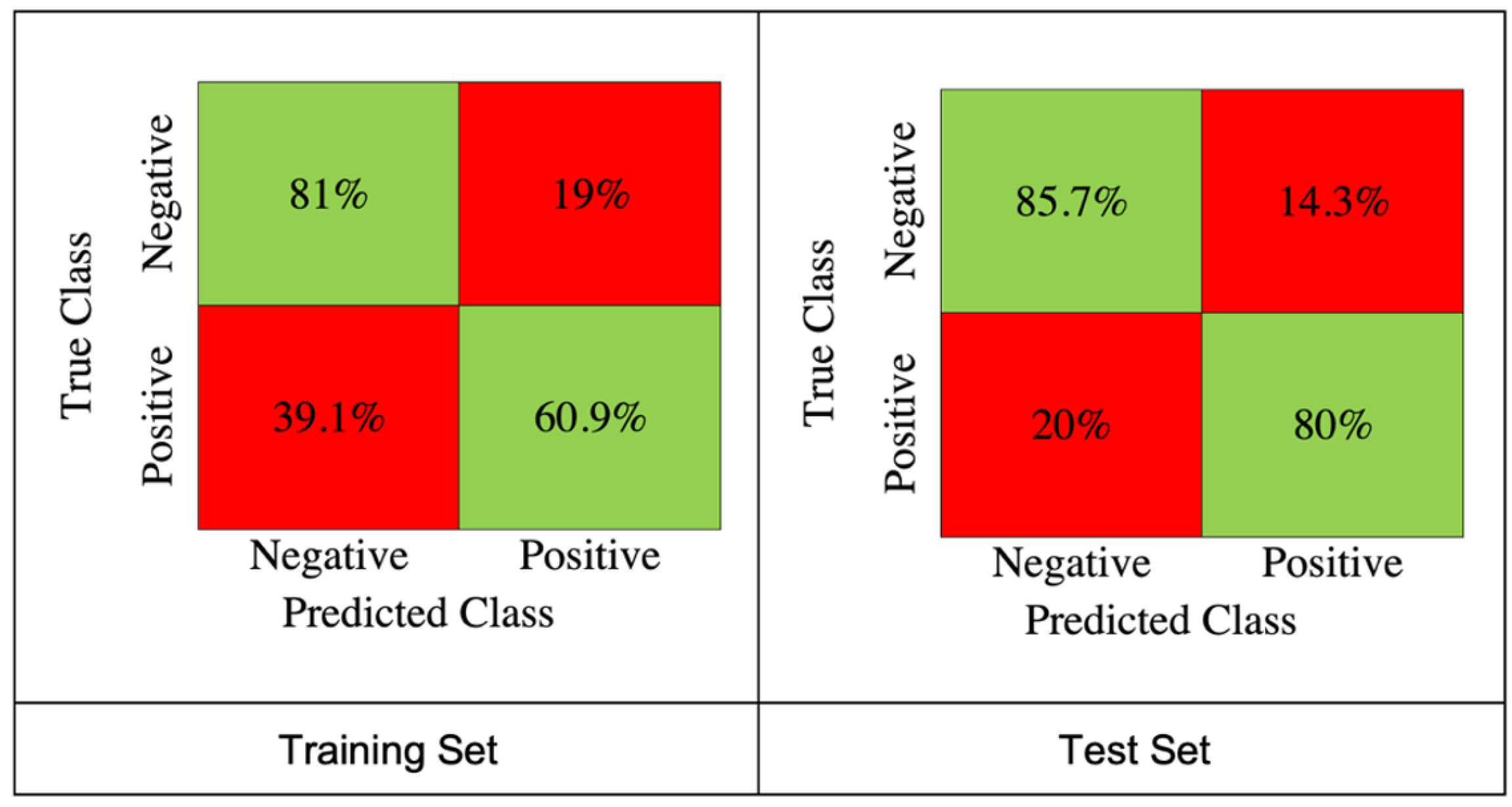
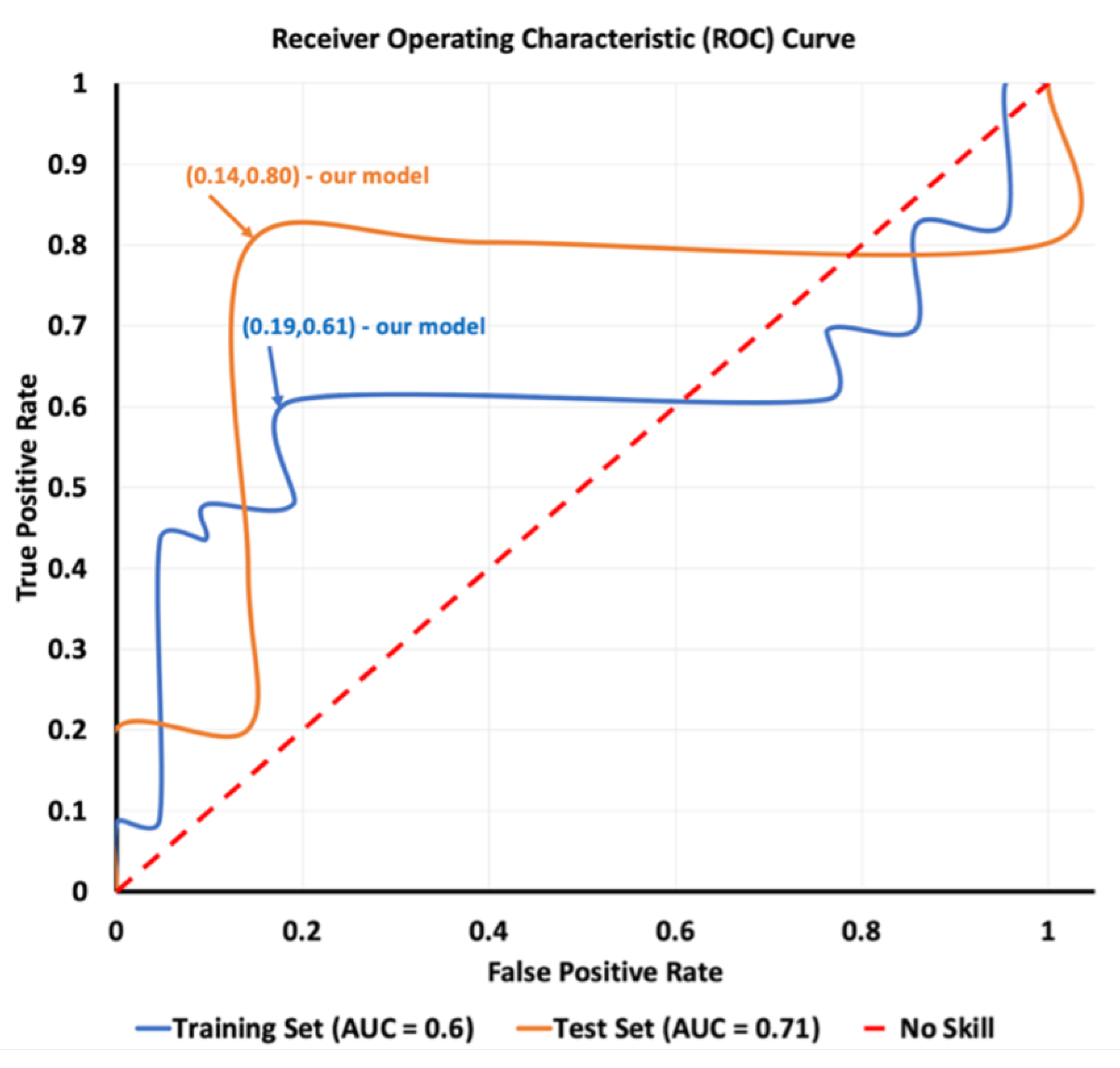
Figure 1. A plot of all the earthquake events with magnitudes larger than Mw 6.8 spread on a global map, taken from our earthquakes dataset. The radius and the color of each earthquake are consistent to the magnitude–yellow corresponds to earthquakes in the range of Mw 6.8–7, orange corresponds to earthquakes in the range of Mw 7–7.9, and red for earthquakes ≥Mw 7.9.
Remotesensing 14 02822 g001
Figure 2. An example of TEC maps for an earthquake day (upper) and for the same earthquake time in the following year (lower), where the red area is the the earthquake’s area, and the red point is the earthquake’s epicenter.
Remotesensing 14 02822 g002
Figure 3. An illustration of the epicenter evaluation process, where the black point is the point to be estimated, and the four red points are the nearest neighbours.
Remotesensing 14 02822 g003
Figure 4. An example of the epicenter time series generation process applied with a 9.1 magnitude earthquake that occurred on 3 November 2011, at 05:46 UTC, where (1–4) are the time series’ of the four nearest points to the epicenter on the map, and (5) is the resulting weighted average time series; the red line is the time of the earthquake.
Remotesensing 14 02822 g004
Figure 5. An example of the result for the daily detrending process applied to the Tōhoku earthquake (11 March 2011), where (1–4) are the time series’ of the four nearest points around the epicenter location, and (5) is the resulting weighted average time series.
Remotesensing 14 02822 g005
Figure 6. An example of the earthquake epicenter time series extraction in different years. The area under the curve marked in red corresponds to a monthly mean SSN number higher than 50 SSN; the area under the curve marked in green corresponds to the monthly mean SSN number lower than 50 SSN. The 9.1 Tōhoku earthquake occurred on 11 March 2011, marked in a red vertical line.
Remotesensing 14 02822 g006
Figure 7. An example of a randomly picked normalized quiet day (3 November 2013) from the quiet days corresponding to the 9.1 Tōhoku earthquake that occurred on 3 November 2011. As can be seen, within a two days time window (before the earthquake event), the normalized ionospheric TEC values exceeded four times the standard deviation of the randomly chosen normalized quiet day.
Remotesensing 14 02822 g007
Figure 8. The confusion matrix for the SVM model results extracted from the training set (left), and the test set (right).
Remotesensing 14 02822 g008
Figure 9. ROC curve of the models we obtained during the hyperparameter optimization process.
Remotesensing 14 02822 g009
Figure 10. A comparison between best model skill scores for each group.
Remotesensing 14 02822 g010
Table 1. Skill score metrics.
PrecisionRecallHSSAccuracyTSS
Training Set
(n = 84)
0.760.6090.4190.70950.419
Test Set
(n = 22)
0.850.80.6570.82850.657
Publisher’s Note: MDPI stays neutral with regard to jurisdictional claims in published maps and institutional affiliations.

