
Relative Strengths Recognition of Nine Mainstream Satellite-Based Soil Moisture Products at the Global Scale


Abstract
:
1. Introduction
2. Datasets and Methods
2.1. Datasets
2.1.1. Satellite-Based Products
2.1.2. ISMN
2.1.3. Auxiliary Datasets
2.2. Methods
2.2.1. Data Quality Control
2.2.2. Assessment Metrics
3. Results
3.1. Evaluations against ISMN Observations
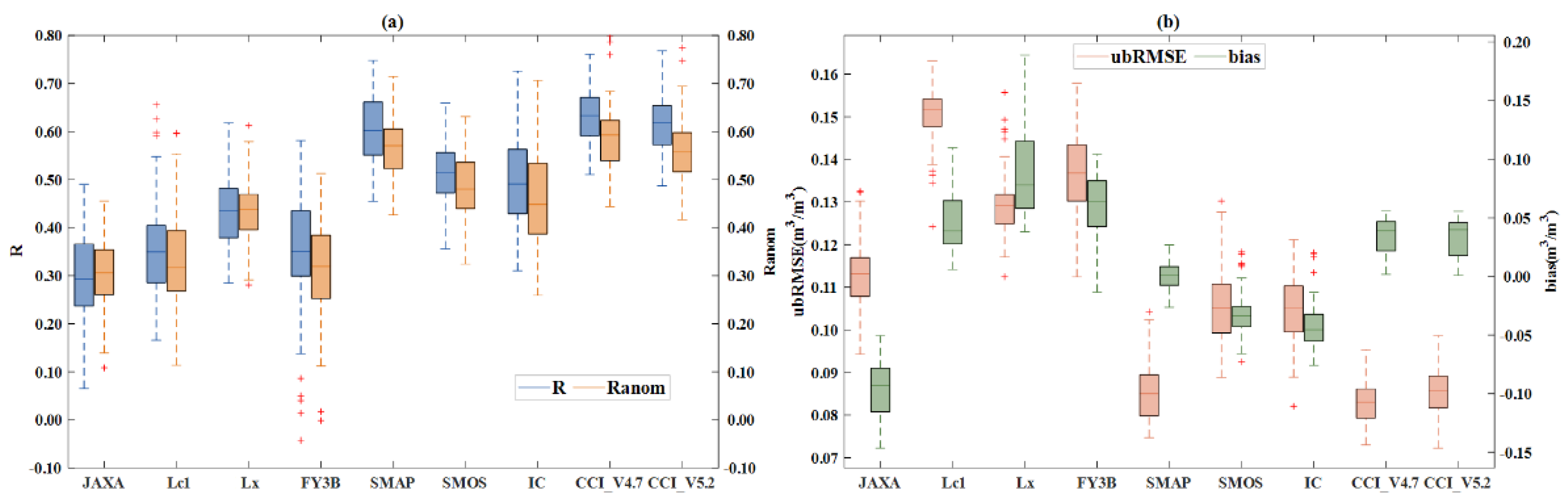
3.1.1. Overall Evaluations
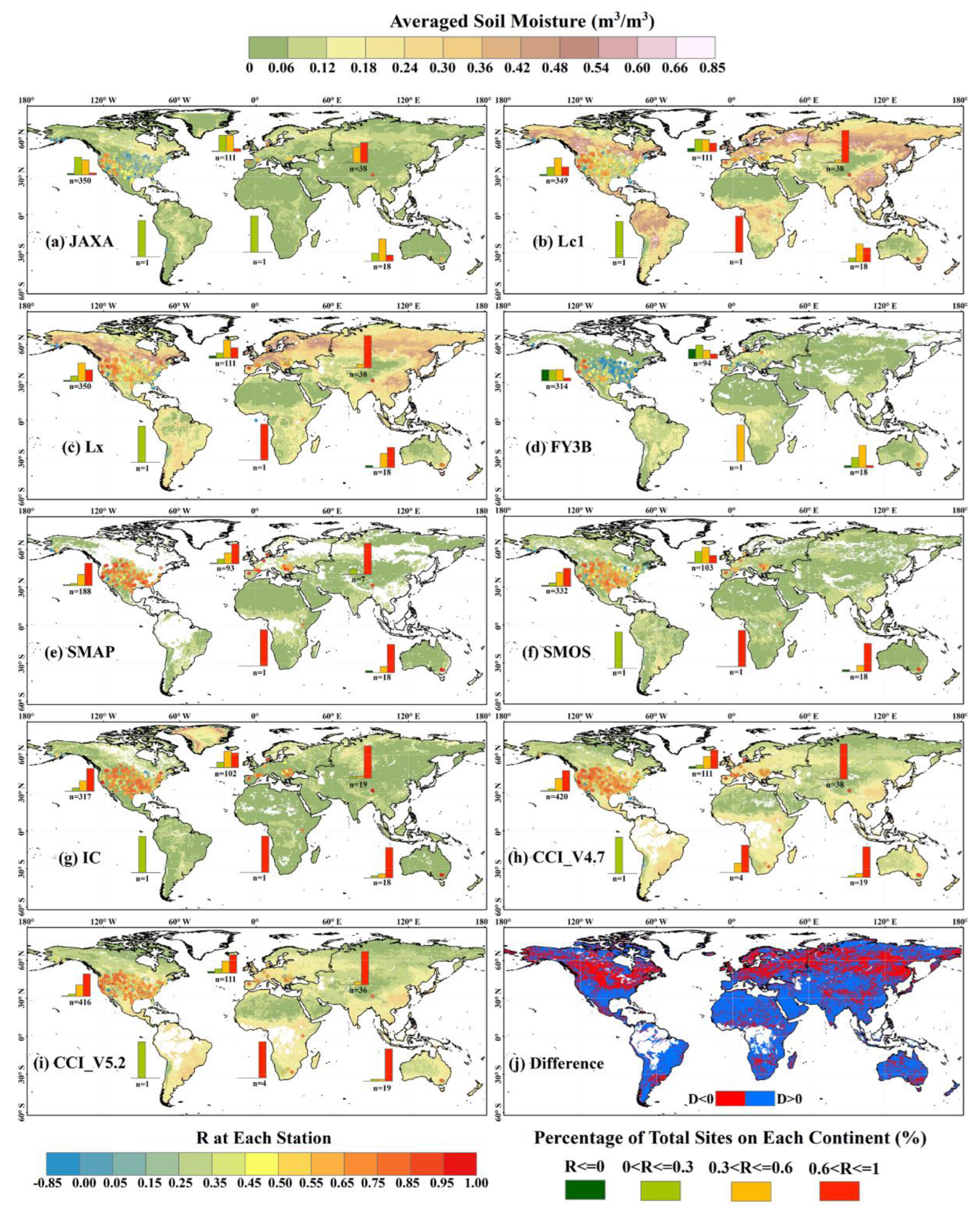
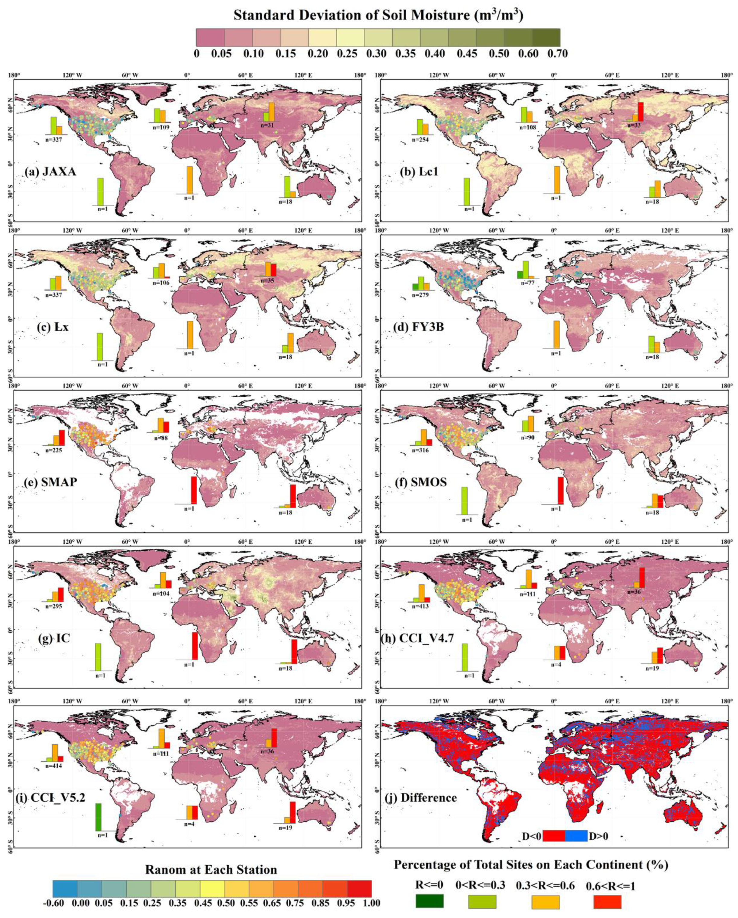
3.1.2. Spatial Patterns of Assessment Metrics
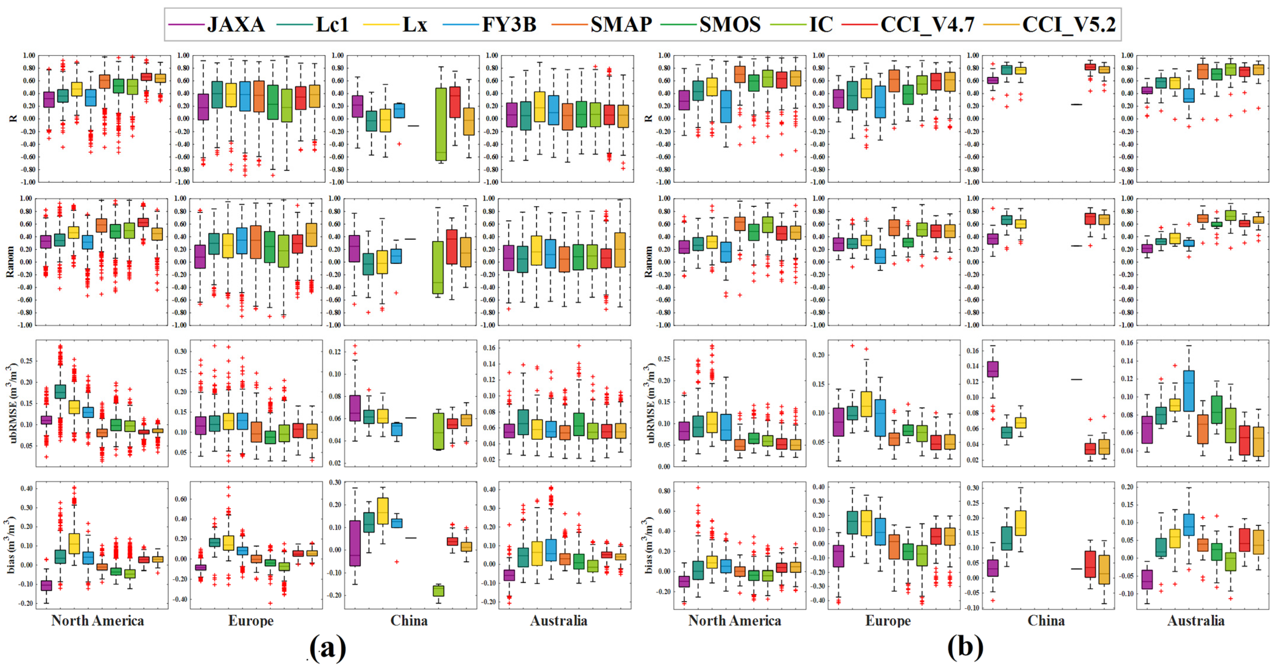
3.1.3. Continent-Level Evaluations
3.2. Evaluations against GLDAS
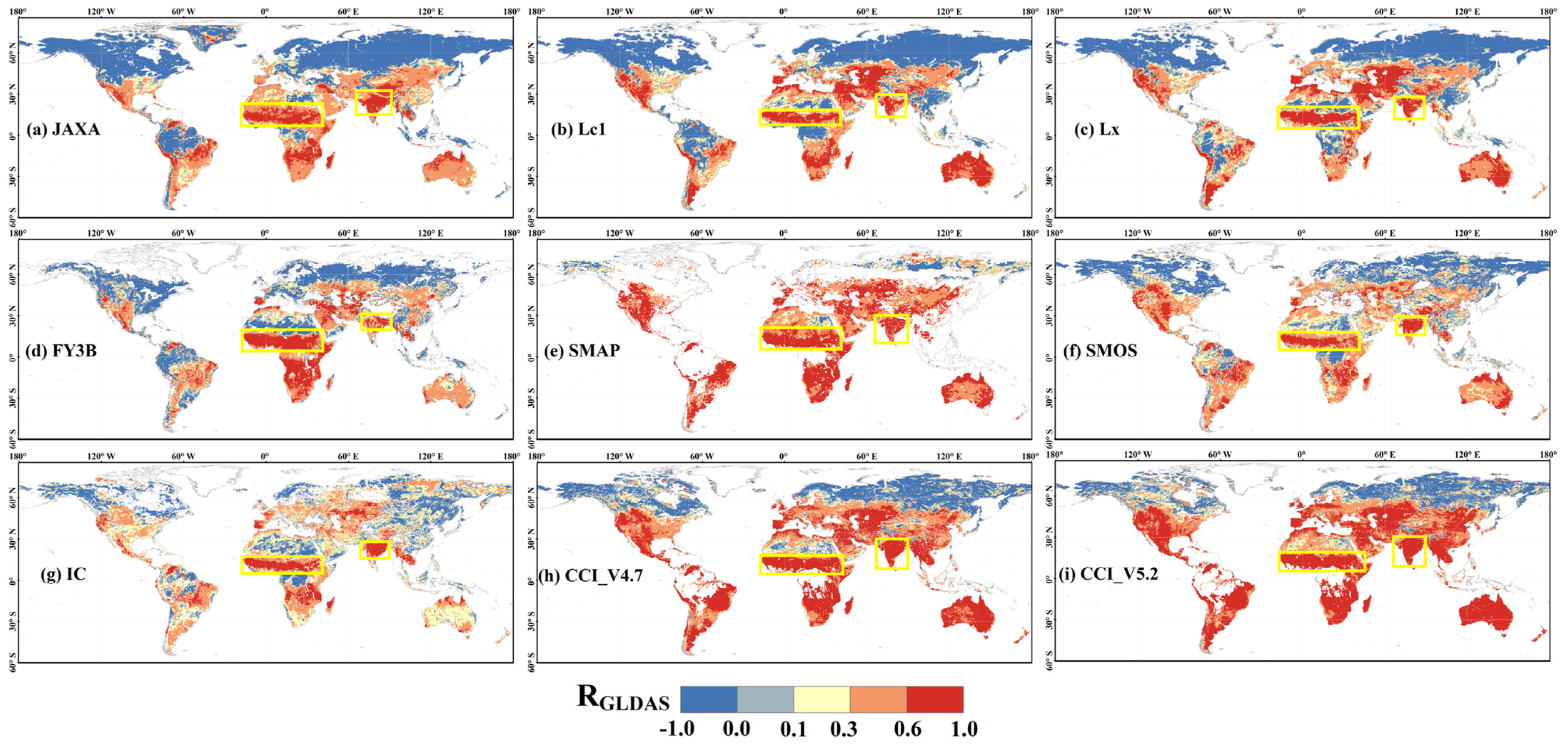
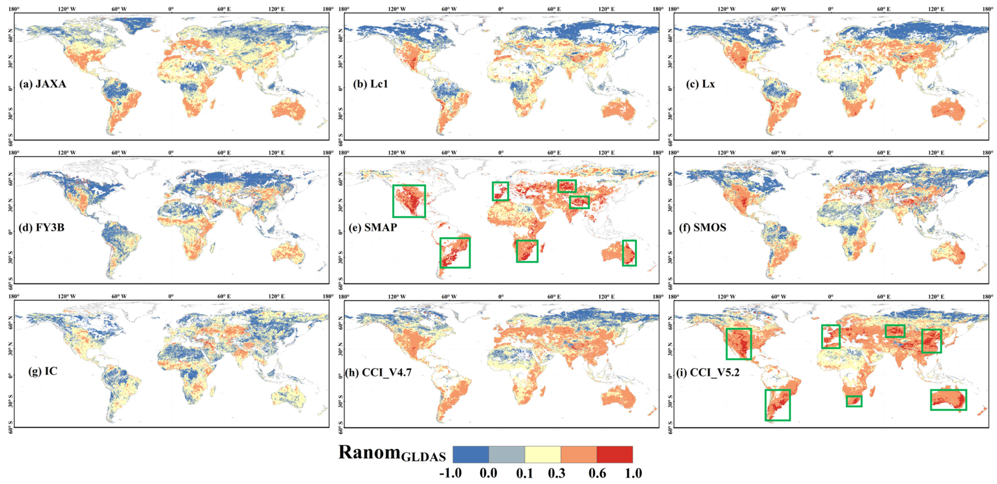
3.2.1. Spatial Patterns of Assessment Metrics
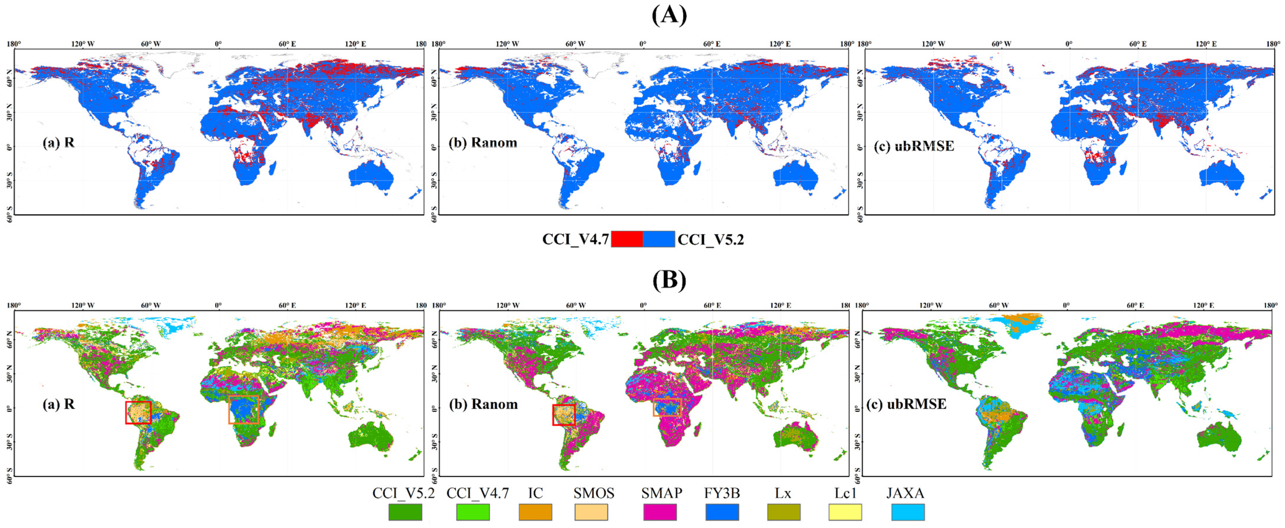
3.2.2. Inter-Comparisons
3.3. Evaluations under Dynamic Conditions
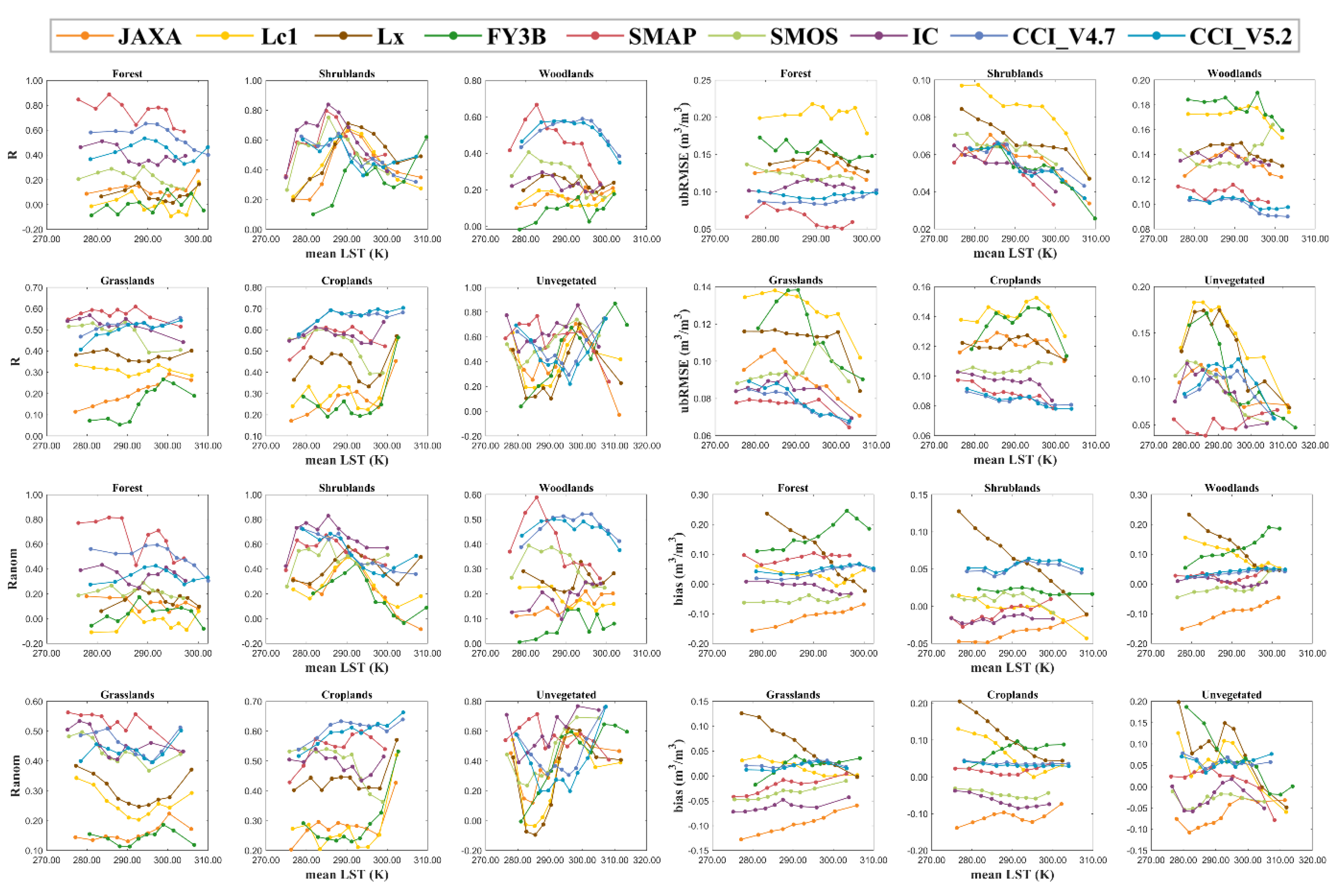
3.3.1. Land Surface Temperature
3.3.2. Soil Moisture
3.3.3. Vegetation Optical Depth
4. Discussion
5. Conclusions
- (1)
- In terms of the overall performance, SMAP and CCI exhibited higher accuracy compared with the other products, followed by SMOS and IC. By contrast, the AMSR2-based products and FY3B showed poorer capabilities with regard to the four metrics, especially the FY3B. In addition, JAXA, SMOS, and IC obviously featured underestimations over the in-situ SM. Temporal sampling had a certain influence on metric scores.
- (2)
- Most products can better capture the temporal dynamics of the original SM than those of SM seasonal anomalies and had higher temporal than spatial performance on all continents. SMOS and IC both had higher uncertainties, mostly in Asia and Europe, due to the impacts of RFI, especially in Europe with R and Ranom < 0.6 at >50% sites. The CCI products outperformed other products considering their abilities in capturing the spatial dynamics of SM anomalies on all continents. The strong variabilities (SD) in SM retrievals were typically accompanied by high random errors and uncertainties (ubRMSE), especially for IC and LPRM-based AMSR2 products.
- (3)
- Compared to SMOS, IC exhibited greater variability and higher random errors in Asia. However, the modification of the IC algorithm improved product performance in Australia. The CCI products had significantly high accuracy in croplands. Compared with the V4.7 product, the inclusion of SMAP enhanced the performance of the V5.2 product in most regions of the world but degraded product accuracy in northeast India. For AMSR2-based products, the Lx outperformed Lc1 and JAXA considering R in most cases. However, based on the performance of ubRMSE and bias, JAXA and Lc1 outperformed Lx, respectively. Therefore, the integration of the three products might improve the value of the AMSR2 mission in SM monitoring.
- (4)
- Considering the dynamic performance with varying LST, all the products presented the highest temporal correlations with both absolutes and anomalies of SM values during 285K–295K in shrublands. In addition, the two CCI products, SMAP, and IC also presented slightly decreased ubRMSE with increasing LST in woodlands, grasslands, and croplands. Under all the LC types, the significant dry biases of JAXA were slowly relieved with increasing LST.
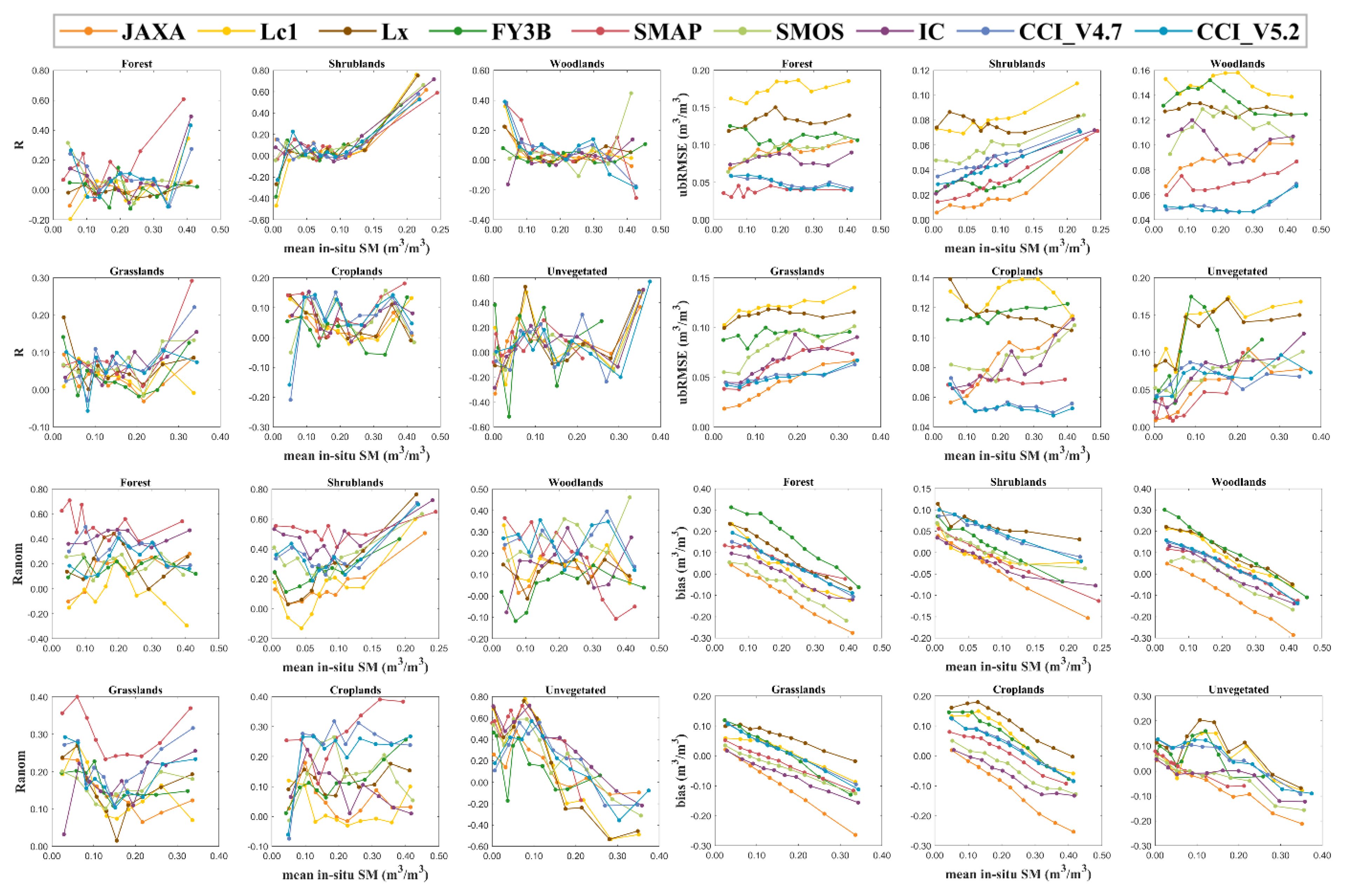
- (5)
- As SM content increased, the bias scores of all the products have nearly linear downward trends with similar declining rates under all the LC types, i.e., the wet bias over in-situ SM gradually turned into dry bias for most products under all the LC types, which revealed a common characteristic of remote sensing SM products; namely, they tended to overestimate the low in-situ SM content but underestimate the high in-situ SM content.
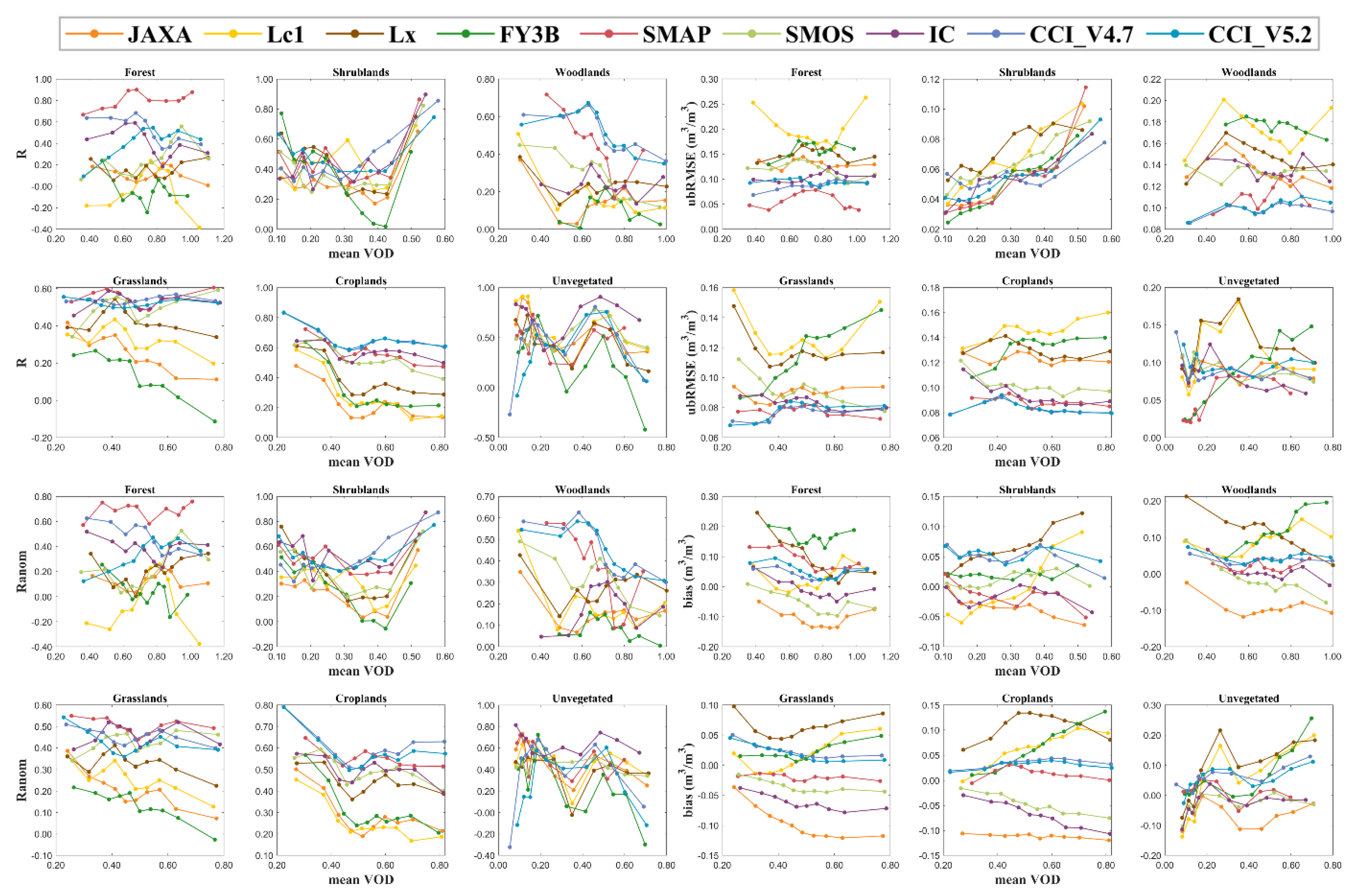
- (6)
- As VOD increased, the AMSR2-based products and FY3B had wider variation ranges in R and Ranom scores than L-band and CCI products in most LC types, which confirmed that the C and X bands were more sensitive to the variation in VOD due to weaker penetration capacity compared with the L-band.
Supplementary Materials
Author Contributions
Funding
Acknowledgments
Conflicts of Interest
References
- Seneviratne, S.I.; Corti, T.; Davin, E.L.; Hirschi, M.; Jaeger, E.B.; Lehner, I.; Orlowsky, B.; Teuling, A.J. Investigating soil moisture—Climate interactions in a changing climate: A review. Earth-Sci. Rev. 2010, 99, 125–161. [Google Scholar] [CrossRef]
- Romano, N. Soil moisture at local scale: Measurements and simulations. J. Hydrol. 2014, 516, 6–20. [Google Scholar] [CrossRef]
- Houser, P.R. Infiltration and soil moisture processes. In Water Encyclopedia; Keeley, J., Ed.; John Wiley & Sons, Inc.: New York, NY, USA, 2005; pp. 493–506. [Google Scholar]
- Entekhabi, D.; Njoku, E.G.; O’Neill, P.E.; Kellogg, K.H.; Crow, W.T.; Edelstein, W.N.; Entin, J.K.; Goodman, S.D.; Jackson, T.J.; Johnson, J.; et al. The Soil Moisture Active Passive (SMAP) Mission. Proc. IEEE 2010, 98, 704–716. [Google Scholar] [CrossRef]
- Kerr, Y.H.; Waldteufel, P.; Wigneron, J.P.; Martinuzzi, J.; Font, J.; Berger, M. Soil moisture retrieval from space: The Soil Moisture and Ocean Salinity (SMOS) mission. IEEE Trans. Geosci. Remote Sens. 2001, 39, 1729–1735. [Google Scholar] [CrossRef]
- Okuyama, A.; Imaoka, K. Intercalibration of advanced microwave scanning radiometer-2. (AMSR2) brightness temperature. IEEE Trans. Geosci. Remote Sens. 2015, 53, 4568–4577. [Google Scholar] [CrossRef]
- Bartalis, Z.; Wagner, W.; Naeimi, V.; Hasenauer, S.; Scipal, K.; Bonekamp, H.; Figa, J.; Anderson, C. Initial soil moisture retrievals from the METOP-A Advanced Scatterometer (ASCAT). Geophys. Res. Lett. 2007, 34, L20401. [Google Scholar] [CrossRef] [Green Version]
- Parinussa, R.M.; Wang, G.; Holmes, T.R.H.; Liu, Y.Y.; Dolman, A.J.; De Jeu, R.A.M.; Jiang, T.; Zhang, P.; Shi, J. Global surface soil moisture from the Microwave Radiation Imager onboard the Fengyun-3B satellite. Int. J. Remote Sens. 2014, 35, 7007–7029. [Google Scholar] [CrossRef]
- Liu, Y.Y.; Parinussa, R.M.; Dorigo, W.A.; De Jeu, R.A.M.; Wagner, W.; van Dijk, A.I.J.M.; McCabe, M.F.; Evans, J.P. Developing an improved soil moisture dataset by blending passive and active microwave satellite-based retrievals. Hydrol. Earth Syst. Sci. 2011, 15, 425–436. [Google Scholar] [CrossRef] [Green Version]
- Liu, Y.Y.; Dorigo, W.A.; Parinussa, R.M.; de Jeu, R.A.M.; Wagner, W.; McCabe, M.F.; Evans, J.P.; van Dijk, A.I.J.M. Trend-preserving blending of passive and active microwave soil moisture retrievals. Remote Sens. Environ. 2012, 123, 280–297. [Google Scholar] [CrossRef]
- Paulik, C.; Dorigo, W.; Wagner, W.; Kidd, R. Validation of the ASCAT Soil Water Index using in situ data from the International Soil Moisture Network. Int. J. Appl. Earth Obs. Geoinf. 2014, 30, 1–8. [Google Scholar] [CrossRef]
- Griesfeller, A.; Lahoz, W.; Jeu, R.; Dorigo, W.; Haugen, L.; Svendby, T.; Wagner, W. Evaluation of satellite soil moisture products over Norway using ground-based observations. Int. J. Appl. Earth Obs. Geoinf. 2015, 45, 155–164. [Google Scholar] [CrossRef] [Green Version]
- McNally, A.; Shukla, S.; Arsenault, K.R.; Wang, S.; Peters-Lidard, C.D.; Verdin, J.P. Evaluating ESA CCI soil moisture in East Africa. Int. J. Appl. Earth Obs. Geoinf. 2016, 48, 96–109. [Google Scholar] [CrossRef] [PubMed] [Green Version]
- Fascetti, F.; Pierdicca, N.; Pulvirenti, L.; Crapolicchio, R.; Muñoz-Sabater, J. A comparison of ASCAT and SMOS soil moisture retrievals over Europe and Northern Africa from 2010 to 2013. Int. J. Appl. Earth Obs. Geoinf. 2016, 45, 135–142. [Google Scholar] [CrossRef]
- Cho, E.; Su, C.H.; Ryu, D.; Kim, H.; Choi, M. Does AMSR2 produce better soil moisture retrievals than AMSR-E over Australia? Remote Sens. Environ. 2017, 188, 95–105. [Google Scholar] [CrossRef]
- Burgin, M.S.; Colliander, A.; Njoku, E.G.; Chan, S.K.; Cabot, F.; Kerr, Y.H.; Bindlish, R.; Jackson, T.J.; Entekhabi, D.; Yueh, S.H. A Comparative Study of the SMAP Passive Soil Moisture Product with Existing Satellite-Based Soil Moisture Products. IEEE Trans. Geosci. Remote Sens. 2017, 55, 2959–2971. [Google Scholar] [CrossRef] [PubMed]
- Ma, H.; Zeng, J.; Chen, N.; Zhang, X.; Cosh, M.H.; Wang, W. Satellite surface soil moisture from SMAP, SMOS, AMSR2 and ESA CCI: A comprehensive assessment using global ground-based observations. Remote Sens. Environ. 2019, 231, 111215. [Google Scholar] [CrossRef]
- Al-Yaari, A.; Wigneron, J.-P.; Dorigo, W.; Colliander, A.; Pellarin, T.; Hahn, S.; Mialon, A.; Richaume, P.; Moran, R.F.; Fan, L.; et al. Assessment and inter-comparison of recently developed/reprocessed microwave satellite soil moisture products using ISMN ground-based measurements. Remote Sens. Environ. 2019, 224, 289–303. [Google Scholar] [CrossRef]
- Wang, Y.; Leng, P.; Peng, J.; Marzahn, P.; Ludwig, R. Global assessments of two blended microwave soil moisture products CCI and SMOPS with in-situ measurements and reanalysis data. Int. J. Appl. Earth Obs. Geoinf. 2020, 94, 102234. [Google Scholar] [CrossRef]
- Zhang, R.; Kim, S.; Sharma, A.; Lakshmi, V. Identifying relative strengths of SMAP, SMOS-IC, and ASCAT to capture temporal variability. Remote Sens. Environ. 2020, 252, 112126. [Google Scholar] [CrossRef]
- Leroux, D.J.; Kerr, Y.H.; Al Bitar, A.; Bindlish, R.; Jackson, T.J.; Berthelot, B.; Portet, G. Comparison between SMOS, VUA, ASCAT, and ECMWF soil moisture products over four watersheds in US. IEEE Trans. Geosci. Remote Sens. 2014, 52, 1562–1571. [Google Scholar] [CrossRef] [Green Version]
- Kim, S.; Liu, Y.Y.; Johnson, F.M.; Parinussa, R.M.; Sharma, A. A global comparison of alternate AMSR2 soil moisture products: Why do they differ? Remote Sens. Environ. 2015, 161, 43–62. [Google Scholar] [CrossRef]
- Cui, Y.; Long, D.; Hong, Y.; Zeng, C.; Zhou, J.; Han, Z.; Liu, R.; Wan, W. Validation and reconstruction of FY-3B/MWRI soil moisture using an artificial neural network based on reconstructed MODIS optical products over the Tibetan Plateau. J. Hydrol. 2016, 543, 242–254. [Google Scholar] [CrossRef]
- Zhu, Y.; Li, X.; Pearson, S.; Wu, D.; Sun, R.; Johnson, S.; Wheeler, J.; Fang, S. Evaluation of Fengyun-3C Soil Moisture Products Using In-Situ Data from the Chinese Automatic Soil Moisture Observation Stations: A Case Study in Henan Province, China. Water 2019, 11, 248. [Google Scholar] [CrossRef] [Green Version]
- Crow, W.T.; Berg, A.A.; Cosh, M.H.; Loew, A.; Mohanty, B.P.; Panciera, R.; de Rosnay, P.; Ryu, D.; Walker, J.P. Upscaling sparse ground-based soil moisture observations for the validation of coarse-resolution satellite soil moisture products. Rev. Geophys. 2012, 50, 1–20. [Google Scholar] [CrossRef] [Green Version]
- Zhang, R.; Kim, S.; Sharma, A. A comprehensive validation of the SMAP Enhanced Level-3 Soil Moisture product using ground measurements over varied climates and landscapes. Remote Sens. Environ. 2019, 223, 82–94. [Google Scholar] [CrossRef]
- Dorigo, W.A.; Wagner, W.; Hohensinn, R.; Hahn, S.; Paulik, C.; Xaver, A.; Gruber, A.; Drusch, M.; Mecklenburg, S.; van Oevelen, P.; et al. The International Soil Moisture Network: A data hosting facility for global in situ soil moisture measurements. Hydrol. Earth Syst. Sci. 2011, 15, 1675–1698. [Google Scholar] [CrossRef] [Green Version]
- Dorigo, W.A.; Xaver, A.; Vreugdenhil, M.; Gruber, A.; Hegyiová, A.; Sanchis-Dufau, A.D.; Zamojski, D.; Cordes, C.; Wagner, W.; Drusch, M. Global Automated Quality Control of in situ Soil Moisture data from the International Soil Moisture Network. Vadose Zone J. 2013, 12, 1–21. [Google Scholar] [CrossRef]
- Dorigo, W.A.; Scipal, K.; Parinussa, R.M.; Liu, Y.Y.; Wagner, W.; de Jeu, R.A.M.; Naeimi, V. Error characterisation of global active and passive microwave soil moisture datasets. Hydrol. Earth Syst. Sci. 2010, 14, 2605–2616. [Google Scholar] [CrossRef] [Green Version]
- Kim, H.; Parinussa, R.; Konings, A.G.; Wagner, W.; Cosh, M.H.; Lakshmi, V.; Zohaib, M.; Choi, M. Global-scale assessment and combination of SMAP with ASCAT (active) and AMSR2 (passive) soil moisture products. Remote Sens. Environ. 2018, 204, 260–275. [Google Scholar] [CrossRef]
- Jackson, T.; Schmugge, T. Vegetation effects on the microwave emission of soils. Remote Sens. Environ. 1991, 36, 203–212. [Google Scholar] [CrossRef]
- Owe, M.; De Jeu, R.; Holmes, T. Multisensor historical climatology of satellite-derived global land surface moisture. J. Geophys. Res. Earth Surf. 2008, 113, 1–17. [Google Scholar] [CrossRef]
- Holmes, T.R.H.; De Jeu, R.A.M.; Owe, M.; Dolman, A. Land surface temperature from Ka band (37 GHz) passive microwave observations. J. Geophys. Res. Earth Surf. 2009, 114, 1–15. [Google Scholar] [CrossRef] [Green Version]
- Yang, H.; Weng, F.; Lv, L.; Lu, N.; Liu, G.; Bai, M.; Qian, Q.; He, J.; Xu, H. The FengYun-3 Microwave Radiation Imager On-Orbit Verification. IEEE Trans. Geosci. Remote Sens. 2011, 49, 4552–4560. [Google Scholar] [CrossRef]
- Soil Moisture Active Passive (SMAP) Algorithm Theoretical Basis Document Level 2 & 3 Soil Moisture (Passive) Data Products. 2020. Available online: https://smap.jpl.nasa.gov/documents/484_L2_SM_P_ATBD_rev_F_final_Aug2020.pdf (accessed on 30 May 2022).
- Brodzik, M.J.; Billingsley, B.; Haran, T.; Raup, B.; Savoie, M.H. EASE-Grid 2.0: Incremental but Significant Improvements for Earth-Gridded Data Sets. ISPRS Int. J. Geo-Inf. 2012, 1, 32–45. [Google Scholar] [CrossRef] [Green Version]
- Wigneron, J.-P.; Jackson, T.; O’Neill, P.; De Lannoy, G.; de Rosnay, P.; Walker, J.; Ferrazzoli, P.; Mironov, V.; Bircher, S.; Grant, J.; et al. Modelling the passive microwave signature from land surfaces: A review of recent results and application to the L-band SMOS & SMAP soil moisture retrieval algorithms. Remote Sens. Environ. 2017, 192, 238–262. [Google Scholar] [CrossRef]
- Fernandez-Moran, R.; Al-Yaari, A.; Mialon, A.; Mahmoodi, A.; Al Bitar, A.; De Lannoy, G.; Rodriguez-Fernandez, N.; Lopez-Baeza, E.; Kerr, Y.; Wigneron, J.-P. SMOS-IC: An Alternative SMOS Soil Moisture and Vegetation Optical Depth Product. Remote Sens. 2017, 9, 457. [Google Scholar] [CrossRef] [Green Version]
- Rodell, M.; Houser, P.R.; Jambor, U.; Gottschalck, J.; Mitchell, K.; Meng, C.-J.; Arsenault, K.; Cosgrove, B.; Radakovich, J.; Bosilovich, M.; et al. The Global Land Data Assimilation System. Bull. Am. Meteorol. Soc. 2004, 85, 381–394. [Google Scholar] [CrossRef] [Green Version]
- Dorigo, W.; Wagner, W.; Albergel, C.; Albrecht, F.; Balsamo, G.; Brocca, L.; Chung, D.; Ertl, M.; Forkel, M.; Gruber, A.; et al. ESA CCI Soil Moisture for improved Earth system understanding: State-of-the art and future directions. Remote Sens. Environ. 2017, 203, 185–215. [Google Scholar] [CrossRef]
- Gruber, A.; Scanlon, T.; van der Schalie, R.; Wagner, W.; Dorigo, W. Evolution of the ESA CCI Soil Moisture climate data records and their underlying merging methodology. Earth Syst. Sci. Data 2019, 11, 717–739. [Google Scholar] [CrossRef] [Green Version]
- Loveland, T.R.; Belward, A. The IGBP-DIS global 1 km land cover data set, DISCover: First results. Int. J. Remote Sens. 1997, 18, 3289–3295. [Google Scholar] [CrossRef]
- Friedl, M.A.; Sulla-Menashe, D.; Tan, B.; Schneider, A.; Ramankutty, N.; Sibley, A.; Huang, X. MODIS Collection 5 global land cover: Algorithm refinements and characterization of new datasets. Remote Sens. Environ. 2010, 114, 168–182. [Google Scholar] [CrossRef]
- Li, D.; Zhao, T.; Shi, J.; Bindlish, R.; Jackson, T.J.; Peng, B.; An, M.; Han, B. First Evaluation of Aquarius Soil Moisture Products UsingIn SituObservations and GLDAS Model Simulations. IEEE J. Sel. Top. Appl. Earth Obs. Remote Sens. 2015, 8, 5511–5525. [Google Scholar] [CrossRef]
- Lievens, H.; Tomer, S.; Al Bitar, A.; De Lannoy, G.; Drusch, M.; Dumedah, G.; Franssen, H.-J.H.; Kerr, Y.; Martens, B.; Pan, M.; et al. SMOS soil moisture assimilation for improved hydrologic simulation in the Murray Darling Basin, Australia. Remote Sens. Environ. 2015, 168, 146–162. [Google Scholar] [CrossRef]
- Cui, C.; Xu, J.; Zeng, J.; Chen, K.-S.; Bai, X.; Lu, H.; Chen, Q.; Zhao, T. Soil Moisture Mapping from Satellites: An Intercomparison of SMAP, SMOS, FY3B, AMSR2, and ESA CCI over Two Dense Network Regions at Different Spatial Scales. Remote Sens. 2018, 10, 33. [Google Scholar] [CrossRef] [Green Version]
- Entekhabi, D.; Reichle, R.H.; Koster, R.D.; Crow, W.T. Performance Metrics for Soil Moisture Retrievals and Application Requirements. J. Hydrometeorol. 2010, 11, 832–840. [Google Scholar] [CrossRef]
- Gruber, A.; De Lannoy, G.; Albergel, C.; Al-Yaari, A.; Brocca, L.; Calvet, J.-C.; Colliander, A.; Cosh, M.; Crow, W.; Dorigo, W.; et al. Validation practices for satellite soil moisture retrievals: What are (the) errors? Remote Sens. Environ. 2020, 244, 111806. [Google Scholar] [CrossRef]
- De Jeu, R.A.M.; Wagner, W.; Holmes, T.; Dolman, A.; van de Giesen, N.; Friesen, J. Global Soil Moisture Patterns Observed by Space Borne Microwave Radiometers and Scatterometers. Surv. Geophys. 2008, 29, 399–420. [Google Scholar] [CrossRef] [Green Version]
- Dente, L.; Ferrazzoli, P.; Su, Z.; van der Velde, R.; Guerriero, L. Combined use of active and passive microwave satellite data to constrain a discrete scattering model. Remote Sens. Environ. 2014, 155, 222–238. [Google Scholar] [CrossRef]
- Chan, S.; Bindlish, R.; O’Neill, P.; Jackson, T.; Njoku, E.; Dunbar, S.; Chaubell, J.; Piepmeier, J.; Yueh, S.; Entekhabi, D.; et al. Development and assessment of the SMAP enhanced passive soil moisture product. Remote Sens. Environ. 2018, 204, 931–941. [Google Scholar] [CrossRef] [Green Version]
- Njoku, E.G.; Ashcroft, P.; Chan, T.K.; Li, L. Statistics and global survey of radio-frequency interference in AMSR-E land observations. IEEE Trans. Geosci. Remote Sens. 2005, 43, 938–947. [Google Scholar] [CrossRef]
- Li, X.; Al-Yaari, A.; Schwank, M.; Fan, L.; Frappart, F.; Swenson, J.; Wigneron, J.-P. Compared performances of SMOS-IC soil moisture and vegetation optical depth retrievals based on Tau-Omega and Two-Stream microwave emission models. Remote Sens. Environ. 2019, 236, 111502. [Google Scholar] [CrossRef]
- De Lannoy, G.J.M.; Koster, R.D.; Reichle, R.H.; Mahanama, S.P.P.; Liu, Q. An updated treatment of soil texture and associated hydraulic properties in a global land modeling system. J. Adv. Model. Earth Syst. 2014, 6, 957–979. [Google Scholar] [CrossRef] [Green Version]
- Liang, Z.; Chen, S.; Yang, Y.; Zhou, Y.; Shi, Z. High-resolution three-dimensional mapping of soil organic carbon in China: Effects of SoilGrids products on national modeling. Sci. Total Environ. 2019, 685, 480–489. [Google Scholar] [CrossRef] [PubMed]
- Bircher, S.; Balling, J.E.; Skou, N.; Kerr, Y.H. Validation of SMOS Brightness Temperatures during the HOBE Airborne Campaign, Western Denmark. IEEE Trans. Geosci. Remote Sens. 2012, 50, 1468–1482. [Google Scholar] [CrossRef] [Green Version]
- Yang, K.; Qin, J.; Zhao, L.; Chen, Y.Y.; Tang, W.J.; Han, M.L.; Lazhu; Chen, Z.Q.; Lv, N.; Ding, B.H.; et al. A Multi-Scale Soil Moisture and Freeze-Thaw Monitoring Network on the Third Pole. Bull. Am. Meteorol. Soc. 2013, 94, 1907–1916. [Google Scholar] [CrossRef]
- Smith, A.B.; Walker, J.; Western, A.W.; Young, R.I.; Ellett, K.M.; Pipunic, R.C.; Grayson, R.B.; Siriwardena, L.; Chiew, F.H.S.; Richter, H.G. The Murrumbidgee soil moisture monitoring network data set. Water Resour. Res. 2012, 48, 1–6. [Google Scholar] [CrossRef]
- Kurc, S.A.; Small, E. Soil moisture variations and ecosystem-scale fluxes of water and carbon in semiarid grassland and shrubland. Water Resour. Res. 2007, 43, 1–13. [Google Scholar] [CrossRef]
- Koster, R.D.; Dirmeyer, P.A.; Guo, Z.; Bonan, G.; Chan, E.; Cox, P.; Gordon, C.T.; Kanae, S.; Kowalczyk, E.; Lawrence, D.; et al. Regions of Strong Coupling Between Soil Moisture and Precipitation. Science 2004, 305, 1138–1140. [Google Scholar] [CrossRef] [Green Version]
- Hornbuckle, B.; England, A. Diurnal Variation of Vertical Temperature Gradients within a Field of Maize: Implications for Satellite Microwave Radiometry. IEEE Geosci. Remote Sens. Lett. 2005, 2, 74–77. [Google Scholar] [CrossRef]
- Level 3 Active/Passive Soil Moisture Product Specification Document. 2015. Available online: https://nsidc.org/sites/files/technical-references/D72551 SMAP L3_SM_P PSD Version 5.1.pdf (accessed on 30 May 2022).
- Parinussa, R.M.; Meesters, A.G.C.A.; Liu, Y.Y.; Dorigo, W.; Wagner, W.; De Jeu, R.A.M. Error Estimates for Near-Real-Time Satellite Soil Moisture as Derived from the Land Parameter Retrieval Model. IEEE Geosci. Remote Sens. Lett. 2011, 8, 779–783. [Google Scholar] [CrossRef]
- Scipal, K.; Holmes, T.; de Jeu, R.; Naeimi, V.; Wagner, W. A possible solution for the problem of estimating the error structure of global soil moisture data sets. Geophys. Res. Lett. 2008, 35, 1–4. [Google Scholar] [CrossRef] [Green Version]
- Wilks, D.S. Statistical Methods in the Atmospheric Sciences, 3rd ed.; Academic Press: Cambridge, MA, USA, 2011. [Google Scholar]
- Wasserstein, R.L.; Lazar, N.A. The ASA’s statement on p-values: Context, process, and purpose. Am. Stat. 2016, 70, 129–133. [Google Scholar] [CrossRef] [Green Version]
- Ma, Z.Q.; Zhou, L.Q.; Yu, W.; Yang, Y.Y.; Teng, H.F.; Shi, Z. Improving TMPA 3B43 V7 datasets using land surface characteristics and ground observations on the Qinghai-Tibet Plateau. IEEE Geosci. Remote Sens. Lett. 2018, 15, 178–182. [Google Scholar] [CrossRef]
- Teng, H.; Shi, Z.; Ma, Z.Q.; Li, Y. Estimating the spatial downscaled rainfall by regression kriging based on TRMM precipitation and DEM in Zhejiang Province, southeast China. Int. J. Remote Sens. 2014, 35, 7775–7794. [Google Scholar] [CrossRef]
- Bell, J.E.; Palecki, M.A.; Baker, C.B.; Collins, W.G.; Lawrimore, J.H.; Leeper, R.; Hall, M.E.; Kochendorfer, J.; Meyers, T.P.; Wilson, T.; et al. U.S. Climate Reference Network Soil Moisture and Temperature Observations. J. Hydrometeorol. 2013, 14, 977–988. [Google Scholar] [CrossRef]
- Bircher, S.; Skou, N.; Jensen, K.H.; Walker, J.P.; Rasmussen, L. A soil moisture and temperature network for SMOS validation in Western Denmark. Hydrol. Earth Syst. Sci. 2012, 16, 1445–1463. [Google Scholar] [CrossRef] [Green Version]
- Calvet, J.-C.; Fritz, N.; Berne, C.; Piguet, B.; Maurel, W.; Meurey, C. Deriving pedotransfer functions for soil quartz fraction in southern France from reverse modeling. SOIL 2016, 2, 615–629. [Google Scholar] [CrossRef] [Green Version]
- Cook, D.R. Soil Temperature and Moisture Profile (STAMP) System Handbook; Technical report; DOE Office of Science Atmospheric Radiation Measurement (ARM) Program: Houston, TX, USA, 2016. [Google Scholar]
- González-Zamora, Á.; Sanchez, N.; Pablos, M.; Martínez-Fernández, J. CCI soil moisture assessment with SMOS soil moisture and in situ data under different environmental conditions and spatial scales in Spain. Remote Sens. Environ. 2018, 225, 469–482. [Google Scholar] [CrossRef]
- Kristine, M.L.; Eric, E.S.; Ethan, D.G.; Andria, L.B.; John, J.B.; Valery, U.Z. Use of GPS receivers as a soil moisture network for water cycle studies. Geophys. Res. Lett. 2008, 35, L24405. [Google Scholar]
- Leavesley, G.H.; David, O.; Garen, D.C.; Lea, J.; Strobel, M.L. A Modeling Framework for Improved Agricultural Water Supply Forecasting. In AGU Fall Meeting Abstracts; American Geophysical Union: Washington, DC, USA, 2008. [Google Scholar]
- Mattar, C.; Santamaria-Artigas, A.; Duran-Alarcon, C.; Olivera-Guerra, L.; Fuster, R.; Borvar’an, D. The lab-net soil moisture network: Application to thermal remote sensing and surface energy balance. Data 2016, 1, 6. [Google Scholar] [CrossRef]
- Moghaddam, M.; Entekhabi, D.; Goykhman, Y.; Li, K.; Liu, M.; Mahajan, A.; Nayyar, A.; Shuman, D.; Teneketzis, D. A Wireless Soil Moisture Smart Sensor Web Using Physics-Based Optimal Control: Concept and Initial Demonstrations. IEEE J. Sel. Top. Appl. Earth Obs. Remote Sens. 2010, 3, 522–535. [Google Scholar] [CrossRef]
- Musial, J.P.; Dabrowska-Zielinska, K.; Kiryla, W.; Oleszczuk, R.; Gnatowski, T.; Jaszczynski, J. Derivation and validation of the high resolution satellite soil moisture products: A case study of the biebrza sentinel-1 validation sites. Geoinformation Issues 2016, 8, 37–53. [Google Scholar]
- Ojo, E.R.; Bullock, P.R.; L’Heureux, J.; Powers, J.; McNairn, H.; Pacheco, A. Calibration and Evaluation of a Frequency Domain Reflectometry Sensor for Real-Time Soil Moisture Monitoring. Vadose Zone J. 2015, 14. [Google Scholar] [CrossRef]
- Schaefer, G.L.; Cosh, M.H.; Jackson, T.J. The USDA Natural Resources Conservation Service Soil Climate Analysis Network (SCAN). J. Atmos. Ocean. Technol. 2007, 24, 2073–2077. [Google Scholar] [CrossRef]
- Wigneron, J.-P.; Dayan, S.; Kruszewski, A.; Aluome, C.; Al-Yaari, A.; Fan, L.; Guven, S.; Chipeaux, C.; Moisy, C.; Guyon, D.; et al. The aqui network: Soil moisture sites in the “les landes” forest and graves vineyards (bordeaux aquitaine region, France). In Proceedings of the IGARSS 2018-2018 IEEE International Geoscience and Remote Sensing Symposium, Valencia, Spain, 22–27 July 2018; pp. 3739–3742. [Google Scholar]
- Zreda, M.; Desilets, D.; Ferré Ty, P.A.; Scott, R.L. Measuring soil moisture content non-invasively at intermediate spatial scale using cosmic-ray neutrons. Geophys. Res. Lett. 2008, 35. [Google Scholar] [CrossRef] [Green Version]
- Zacharias, S.; Bogena, H.; Samaniego, L.; Mauder, M.; Fuß, R.; Pütz, T.; Frenzel, M.; Schwank, M.; Baessler, C.; Butterbach-Bahl, K.; et al. A Network of Terrestrial Environmental Observatories in Germany. Vadose Zone J. 2011, 10, 955–973. [Google Scholar] [CrossRef] [Green Version]


| Dimensions | Metrics | North America | Europe | China | Australia |
|---|---|---|---|---|---|
| Spatial | R | CCI_V4.7 | Lc1 | CCI_V4.7 | Lx |
| Ranom | CCI_V4.7 | CCI_V5.2 | CCI_V4.7 | CCI_V5.2 | |
| ubRMSE | CCI_V4.7 | SMOS | IC | SMAP | |
| bias | SMAP | SMAP | CCI_V5.2 | SMOS | |
| Temporal | R | SMAP | SMAP | CCI_V4.7 | IC |
| Ranom | SMAP | SMAP | CCI_V4.7 | IC | |
| ubRMSE | SMAP | CCI_V5.2 | CCI_V4.7 | CCI_V5.2 | |
| bias | SMAP | SMAP | CCI_V5.2 | IC |
Publisher’s Note: MDPI stays neutral with regard to jurisdictional claims in published maps and institutional affiliations. |
© 2022 by the authors. Licensee MDPI, Basel, Switzerland. This article is an open access article distributed under the terms and conditions of the Creative Commons Attribution (CC BY) license (https://creativecommons.org/licenses/by/4.0/).
Share and Cite
Min, X.; Shangguan, Y.; Huang, J.; Wang, H.; Shi, Z. Relative Strengths Recognition of Nine Mainstream Satellite-Based Soil Moisture Products at the Global Scale. Remote Sens. 2022, 14, 2739. https://doi.org/10.3390/rs14122739
Min X, Shangguan Y, Huang J, Wang H, Shi Z. Relative Strengths Recognition of Nine Mainstream Satellite-Based Soil Moisture Products at the Global Scale. Remote Sensing. 2022; 14(12):2739. https://doi.org/10.3390/rs14122739
Chicago/Turabian StyleMin, Xiaoxiao, Yulin Shangguan, Jingyi Huang, Hongquan Wang, and Zhou Shi. 2022. "Relative Strengths Recognition of Nine Mainstream Satellite-Based Soil Moisture Products at the Global Scale" Remote Sensing 14, no. 12: 2739. https://doi.org/10.3390/rs14122739