Article

Estimation of Corn Latent Heat Flux from High Resolution Thermal Imagery

1
Department of Agricultural and Biological Engineering, Purdue University, West Lafayette, IN 47907, USA
2
Wabash, Lafayette, IN 47905, USA
*
Author to whom correspondence should be addressed.
Remote Sens. 2022, 14(11), 2682; https://doi.org/10.3390/rs14112682
Submission received: 21 April 2022 / Revised: 27 May 2022 / Accepted: 30 May 2022 / Published: 3 June 2022
(This article belongs to the Topic Remote Sensing in Water Resources Management Models)

Abstract

:
Crop evapotranspiration (ET), which is directly related to latent heat flux, is also a key indicator in determining the water status of crops. In order to estimate the latent heat flux, two-source energy balance (TSEB) models have been developed for thermal imagery from satellite platforms. However, because of the coarse resolution of thermal sensors on the satellite, distinguishing soil and vegetation is difficult which complicates the calculation process and introduces errors in latent heat estimates. In this research, high-resolution thermal datasets (0.05 m) and corresponding RGB datasets (0.03 m) were used for calculating crop latent heat flux using an adapted TSEB model. The RGB datasets were used for supervised classification of soil and vegetation, and the classification results were then used to filter the thermal mosaics to separate vegetation and soil temperatures. The vegetation temperature is used for calculating latent heat flux and the results are validated against the ground reference measurements of latent heat using a handheld porometer. The objective of this research is to introduce a workflow including an adapted TSEB model which is customized for high resolution thermal images from unmanned aircraft systems (UAS) to estimate the latent heat flux of row crops in agricultural fields. Nine dates of data collection in 2018 and 2020 have been evaluated and the root mean square error (RMSE) varies between 16 to 106 W/m2 depending on the days after planting (DAP) and the time of measurement for each day. The results indicate that the workflow introduced here is able to provide estimates of instantaneous latent heat flux (evapotranspiration) measurements for row crops in agricultural fields which will enable people to make reliable decisions related to irrigation scheduling.

Graphical Abstract

1. Introduction

Crop evapotranspiration (ET), which transfers a large volume of water into the atmosphere from the combination of evaporation (E) from soil, water bodies, vegetated surfaces and transpiration (T), which is a fundamental part of the photosynthesis process in plants, is directly related to latent heat flux (latent heat flux is converted to ET by dividing by λ × ρw, where λ is the latent heat of vaporization and ρw is the density of water) [1] and has played a key role in determining the water status of crops, thus serving as an important indicator for management of irrigation and water resources in areas of water scarcity [2,3]. ET estimation is critical for addressing immediate needs at farm scales, including improved crop water management and irrigation efficiencies, weather and crop-stress forecasting, and decision-support tools as water supplies become increasingly constrained in the 21st century [4].
The primary controls on ET are energy inputs such as incoming solar radiation and the capacity of the air to hold more water vapor both from local water vapor (humidity) and from mixing with drier air controlled by wind speed. Air temperature has a less direct impact on the ET rate (latent heat flux) because it affects the water holding capacity of the air and it is therefore highly correlated with both solar radiation and ET. Other factors such as different growing stages for the agricultural crops, soil and management factors (soil’s water content, its water characteristic curve and available soil water content) can also affect the latent heat flux [1,5,6].
Traditional measurement systems for crop ET include: (1) lysimetry, which measures evaporation and transpiration based on the change in weight of a lysimeter where weight change is associated with the change in soil water storage once precipitation and drainage are removed [7,8]; (2) eddy covariance systems that directly quantify ET by measuring three-dimensional wind velocities and water vapor content of air fluxes at very high resolutions [9,10]; and (3) Bowen ratio energy balance systems that indirectly quantify ET by measuring net radiation, soil heat flux and vapor pressure at two different heights and apply the Bowen ratio energy balance equation [11]. Each of these methods require great care and expense to collect accurate measurements for inputs and are very limited in the spatial area for which they are representative.
In 1948, Penman [12] combined the energy balance with the mass transfer method and derived an equation to compute the evaporation from an open water surface from standard climatological records of sunshine, temperature, humidity and wind speed. This method was further developed and extended to cropped surfaces by introducing resistance factors. In 1990, the United Nation’s Food and Agriculture Organization (FAO) recommended the adoption of the Penman-Monteith combination method as a new standard for reference evapotranspiration and advised on procedures for calculation of the various parameters [5]. However, these measurements are very labor intensive and require substantial time for data collection and sensor maintenance. Their measurement footprints are also very limited, so they cannot meet the increasing needs to have high-resolution spatially explicit measurements for mapping field, regional and meso scale patterns of ET on the Earth’s surface. The variability of ET also makes it very difficult for any sort of interpolation and extrapolation based on the values from the coverage area. In this case, remote sensing platforms (unmanned aircraft systems and satellites) with thermal sensors installed have been used for this purpose more often recently [1,2,13,14].
Surface energy balance models are based on balancing net radiation with ground heat flux, sensible heat flux and latent heat flux assuming that heat advection is negligible [15]. Surface temperature estimates from those remote sensing systems can be used in the models to indirectly estimate sensible heat flux, net radiation and ground heat flux using some local weather data, and in this way, latent heat flux can be solved as the residual. Such models can be used to estimate latent heat over large areas without significant investment in specialized equipment and may be the only approach available for ungauged areas where man-made measurements are extremely difficult to conduct.
Original development of these energy balance models assumed a single incoming energy source at the land surface, effectively representing the land surface as covered by a single big leaf. Norman et al. [16] introduced an iterative method known as the Two-Source Energy Balance (TSEB) model that includes energy transfer from the soil to the vegetation as a separate, second source of energy to more accurately calculate the joint latent heat flux of the plant canopy and soil. This method uses remote sensing measurements of surface directional brightness temperature and some ancillary data (weather parameters such as air temperature, humidity, wind speed and ground measurements like soil temperature, and leaf area index (LAI)). Since brightness temperature measurements are typically available only at a single viewing angle, a Priestly-Taylor approximation [17] is used to acquire an initial estimation of canopy temperature, and then latent heat flux can be calculated in an iterative manner. Because the TSEB was developed for satellite remote sensing systems, it suffers from a lack of fine spatial resolution data to distinguish between soil and plants and fine scale temporal data to monitor the water status of crops in real time.
The potential to adapt the TSEB method to data collected from unmanned aircraft systems (UAS) can reduce the limitations of satellite-based ET estimates by obtaining imagery with centimeter level spatial resolution and the potential to collect imagery several times a week or even within the same day as needed. For example, Brenner et al. [18] mapped latent heat flux from a grass site with land surface temperature acquired from UAS as an input to both one and two-source energy balance models. They collected thermal imagery with a spatial resolution of 6 cm during the months of June and July. When comparing the simulated latent heat flux from these models with coincident eddy covariance measurements, they found that the two-source model, with a more complex treatment of the energy and surface temperature partitioning between the soil and vegetation, outperformed the simpler one-source model in estimating sensible and latent heat fluxes. Norman et al. [19] developed the dual-temperature-difference (DTD) model by incorporating two temperature observations into the TSEB modelling scheme: one conducted an hour after sunrise and another conducted later the same day when flux estimations were desired. Hoffmann et al. [15] compared the performance of two dual-source models (TSEB and DTD) by using land surface temperature (LST) from mosaics of thermal imagery from UAS with a spatial resolution of 0.2 m as an input to the models. They found that both TSEB and DTD simulations agreed with eddy covariance measurements. The DTD model results were better, but significantly limited its potential use given the need for two acquisitions per day rather than one.
One of the main sources of error for the TSEB model derives from the estimation of canopy and soil temperature through an iterative process rather than from direct measurements. Ortega-Farías et al. [20] incorporated thermal and multispectral imagery into a remote sensing energy balance (RSEB) algorithm to simulate net radiation, soil, sensible and latent heat fluxes in an olive orchard. They separated canopy and soil surfaces from imagery manually by using discrimination and segmentation supervised techniques. With this technique they found that the simulated values were generally in agreement with flux measurements from an eddy covariance system. All of their data acquisitions occurred near solar noon. Riveros-Burgos et al. [21] applied a clumped model developed by Brenner and Incoll [22] to estimate olive orchard evapotranspiration using high resolution thermal imagery. They found that the estimated values were in accord with the ground-based measurements while the main disagreements were associated with olive trees under moderate water stress and high atmospheric demand for water vapor. In order to distinguish between canopy and soil temperature, the K-means clustering algorithm was applied to the thermal orthomosaics and a binary raster was created with two clusters where pixels were classified for canopy and soil. However, this classification may cause a problem since under many conditions there is no clear difference in temperature values between soil and canopy.
Previous research indicates the potential of using high resolution thermal imagery along with an energy balance model for calculating the latent heat flux of orchard or grass, but little research has been done to test the performance of the model on row crops. Also, the model has only been tested under a certain illumination condition and on a relatively coarse resolution, so to what extent the models can be applied to higher resolution imagery is still questionable. Partitioning between the canopy and soil is always important, since calculations of energy components of these two will require different sets of equations, and this was done previously by using the NDVI and temperature difference [21,23]. However, under field conditions, the temperature difference of the two is not certain and also the NDVI threshold values for the vegetation and soil are empirical and will result in errors from day to day.
The objective of this research is to introduce a workflow including using an adapted TSEB model, customized for high resolution thermal images from UAS, to estimate latent heat flux from row crops in agricultural fields. In this research, very high-resolution thermal datasets (0.05 m) and corresponding RGB datasets (0.03 m) were used for calculating crop latent heat flux. The RGB datasets were used for supervised classification of soil and vegetation, and the classification results were then used to filter the thermal mosaic to separate vegetation and soil temperatures, after which the vegetation temperature was used for calculating the latent heat flux. Finally, the results were validated against in situ porometry measurements as well as latent heat flux calculated from the Penman-Monteith (PM) equation using local weather data. Multiple flights are processed using the model, and the variance of latent heat flux between different days from a single growing season is assessed using supplementary information including weather parameters.

2. Materials and Methods
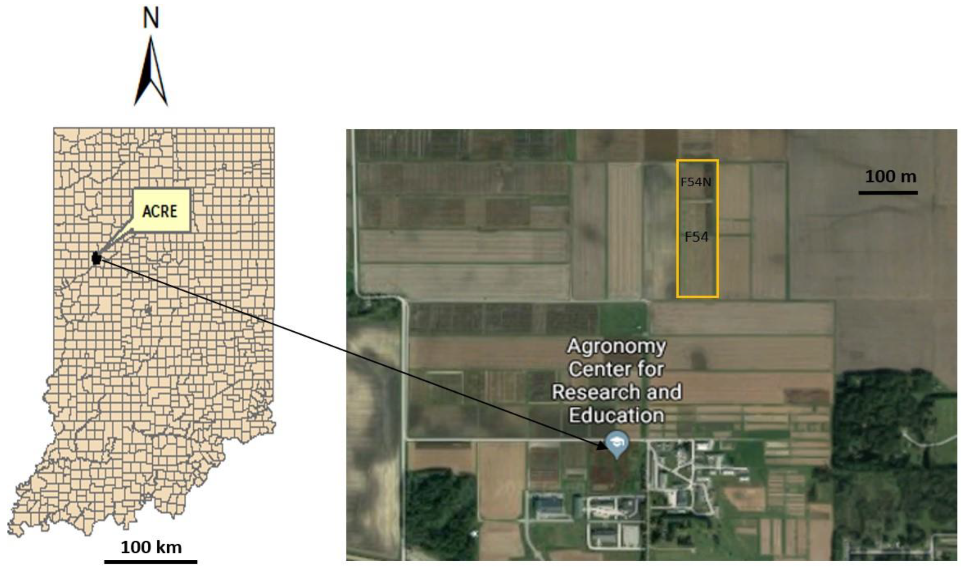
2.1. Field Site

Data was collected in the summer of 2018 and 2020. All of the flights took place at the Agronomy Center for Research and Education (ACRE), a research farm operated by Purdue University. A mixture of corn and sorghum fields identified as “field 54” (40°28′44.98″N, 86°59′23.57″W) (Figure 1) is the target for all flights. This field is about 5 hectares and was set up to support breeding experiments, with one or more experiments established in it every other year, with each experiment consisting of hundreds to thousands of smaller plots with specific genotypes of sorghum or corn.
The air temperature, relative humidity, solar radiation, precipitation, and wind speed are measured at 30-min intervals using an automatic meteorological station located near the experimental site (500 m away). These data were used to calculate the hourly reference latent heat flux according to the Penman-Monteith model [5] and were also used as inputs to the modified TSEB model for calculating latent heat flux from UAS imagery.

2.2. Remote Sensing Data Acquisition and Processing

A FLIR DUO Pro R camera (FLIR Systems, Wilsonville, OR, USA) and a ThermalCapture Fusion Zoom camera (TeAx, Wilnsdorf, Germany) were used to capture all thermal infrared imagery used in this analysis. Each of these cameras consists of two sensors: a thermal infrared imager and a visible-light imager. The thermal imagers are the same, with a resolution of 640 × 512 and a focal length of 19 mm with a field of view 32° × 26°. Both thermal imagers are sensitive to spectral wavelengths from 7.5 to 13.5 µm. Their measurement accuracy is ±5 °C or 5% of the reading in its operating temperature range (20 °C to +50 °C). The visible-light imager of FLIR DUO Pro R has a resolution of 4000 × 3000, while that of ThermalCapture Fusion Zoom is 1920 × 1080 and has a 10 times optical zoom. Both cameras have been calibrated in the lab using methods described in Zhu et al. [24].
The FLIR camera was mounted on the underside of a DJI M200 Drone, and the ThermalCapture Fusion Zoom camera was mounted on the underside of a DJI M600 Drone (Shenzhen, China) with a gimbal so that nadir images were collected during flights. Flights were conducted at a height of 60 m so that the ground sampling distance is about 5.4 cm per pixel for the imagery from both thermal imagers, and 3.3 cm per pixel for the visible imagery from the FLIR camera and 4.2 cm per pixel from ThermalCapture camera. The speed of the M200 drone was 5.6 m/s and that of M600 was 7.5 m/s. The spacing between flight paths was set to be 6.8 m for both drones to achieve a frontal overlap of 80% and 95% for thermal images from FLIR and ThermalCapture and a side overlap of 80%. The ThermalCapture camera takes still images at a frame rate of 5 fps. ThermalViewer (TeAx, Germany) software was used for extracting thermal and RGB frames from the ThermalCapture camera. Most of the flights were conducted in the afternoon around 2:00 p.m. to 4:00 p.m. to provide for stable air temperature conditions.
Pix4D mapper software (Pix4D S.A., Prilly, Switzerland) was used for creating mosaics for both RGB and thermal datasets. The mosaics of these two datasets on the same day and same flight were then registered to each other in ENVI (L3Harris Geospatial, Broomfield, CO, USA) using ground control points deployed around the field. The RGB images were used as the base images for warping the corresponding thermal images. Four other GCPs on each side of the field which were not used in the coregistration process were used for accuracy evaluation. The RMSE for both horizontal and vertical directions of these GCPs in both images have been calculated for evaluating the accuracy of registration.
After the registration, areas of interest (an area within the field usually contains multiple plots in the shape of rectangle) were extracted from the full mosaic image. A supervised classification workflow in ENVI was run on the RGB images. The Mahalanobis Distance algorithm [25] was selected to provide a conservative result which largely avoided misclassifying soil pixels into vegetation pixels but may ignore some dark vegetation pixels. The classification accuracy was evaluated by a confusion matrix method as described by Lillesand et al. [26]. More than 100 points were selected randomly between classification results and original images for three classes: dark soil, sunlit soil, and crops. These points were used to compute the producer and user accuracies of the classified imagery. The classification results were then overlaid on the corresponding thermal images as a mask to separate vegetation from soil, as only the vegetation temperature is used for calculating latent heat flux.
Canopy temperature and soil temperature are directly acquired from the high-resolution thermal imagery. Thermal imagery was calibrated by on-site water targets to get accurate temperature measurements [24].

2.3. Two-Source Energy Balance (TSEB) Model

Instead of treating the land surface as a big leaf with a single uniform layer as was done with the original one source energy balance (OSEB) models, the TSEB model distinguishes between the surface energy transfer of soil and vegetation sub-systems and requires soil and canopy surface temperatures to solve the energy budgets of these layers separately [27,28] which improves the accuracy of the resulting latent heat flux estimates. An overview of the critical components of the TSEB employed in this research is provided below, along with a discussion of how the model was modified and employed for this project.
The canopy and soil energy balance are described as:
R N = G + H + L E
In which R N is the net radiation, G is the soil heat conduction flux; H is the sensible heat flux and L E is the latent heat flux. The above Equation (1) is particularly useful for quantifying energy fluxes in satellite imagery; however, with high resolution thermal imagery becoming more available these days, vegetation and soil can be separated in imagery and surface energy fluxes calculated separately. Because the focus of this study is on LE from crops, only the canopy energy balance equations are discussed below.
The latent heat flux of the canopy is calculated with the following equations.
L E C = R n , C A N O P Y H C
In which, R n , C A N O P Y is the canopy net radiation and H C is the sensible heat flux of the canopy. Canopy net radiation is simply the balance between incoming and outgoing shortwave and longwave radiation. Canopy net shortwave radiation consists of two components: net direct radiation and net diffuse radiation, and is estimated as the sum of direct visible radiation, diffuse visible radiation, direct near infrared radiation and diffuse near infrared radiation [29,30,31]. For this application, the use of high-resolution thermal imagery required modifications to the original methodology specifically for the estimation of net longwave radiation and atmospheric stability. These modifications are detailed in the following sections.

2.3.1. Longwave Radiation

The net longwave radiation on the canopy, where incoming longwave radiation from the sky and soil is balanced by outgoing longwave radiation from the canopy itself, is calculated using [29]:
L N , C = [ 1 τ b t ( ψ ) ] [ L s k y + L S 2 L C ]
where L s k y , L C and L S are longwave radiation (W/m2) from the sky canopy and soil, respectively. ψ is the wavelength of energy and τ b t ( ψ ) is the percent of total beam radiation (direct and down scattered) transmitted through the canopy, which is computed as:
τ b t ( ψ ) = exp ( α K b e ( ψ ) L t )
in which α is the leaf absorptivity; K b e ( ψ ) is the extinction coefficient which depends on the canopy structure and the beam zenith angle; L t is the depth of the canopy. Longwave radiationfrom the sky and canopy are calculated using the Stefan-Boltzmann law based on their observed temperatures. Most of the thermal images acquired are nadir images, which means that much of the soil is obscured by the canopy at later growth stages, and this part of the soil cannot be separated by the classification algorithm. Since the soil is completely shaded, L s is calculated using the minimum values of neighboring soil temperature measurements of the target vegetative surface.

2.3.2. Monin-Obukhov Similarity Theory

Monin-Obukhov similarity theory describes the non-dimensionalized mean flow and mean temperature in the surface layer under non-neutral conditions as a function of the dimensionless height parameter [32]. Obukhov stability length is defined as [29,33]:
L = u * 3 L c o n s t a n t ( H v ρ c p )
where u * is friction velocity (m/s), H v is the virtual sensible heat flux (W/m2), ρ is the density of air (kg/m3), c p is the heat capacity of air (J kg−1 °C−1); L c o n s t a n t is expressed as follows:
L c o n s t a n t = k g T A
where k is von Karman’s constant (≈0.4), g is the acceleration of gravity (m/s2) and T A is the air temperature at the time of measurement.
The relationship between virtual sensible heat flux, sensible heat flux and latent heat flux is defined as:
H v = H C + ( 0.61 × T A × c p × L E C λ )
In which, λ is the latent heat of vaporization, L E C (W/m2) is the latent heat flux and H C is the sensible heat flux (W/m2). In this research, the latent and sensible heat flux are assumed to be for vegetation.
The aerodynamic resistance is expressed as:
R A = [ ln ( z U d z M ) Ψ m ] [ ln ( z T d z M ) Ψ h ] 0.16 U
where z U and z T are the height of wind speed measurement U and air temperature measurement. Ψ m and Ψ h are the diabatic correction factors for momentum and heat. d is displacement height ( d 0.65 h C , where h C is canopy height.) z M is the roughness length for momentum ( z M 0.125 h C ).
When leaves are cooler than the air, the atmosphere is stable, and the direction of sensible heat flux is downward with a negative sign. In that case, the following Equation (9) is used to calculate Ψ m and Ψ h [33]:
Ψ m ( ζ ) = Ψ h ( ζ ) = 5 ζ
Otherwise, if the atmosphere is unstable, empirical linear equations, which are a simplified version of original equations, are used:
Ψ m = 2.486 ζ + 0.0036
Ψ h = 5.624 ζ + 0.0449
where ζ is defined in the following Equation (12):
ζ = h c d L
Substituting the above results into the equation for R A (Equation (8)), R A can be expressed as a parameter with only one unknown value which is the canopy sensible heat flux.
The canopy sensible heat flux can be calculated as [16]:
H C = ρ c P T C T A R A
Latent heat flux can then be calculated by substituting the sensible heat flux into Equation (2).

2.4. Ground-Based Latent Heat Estimates

Given the difficulty of measuring small-scale ET directly from a large field, two methods were used to provide ground reference for the UAS-based latent heat estimates. These were the calculation of ET using the Penmen-Monteith method and local atmospheric conditions, and the direct measurement of stomatal conductance from a number of plants within the field experiment to provide localized ET measurements. More about each of these methods is provided below.

2.4.1. Penmen-Monteith Estimation of Canopy ET

Hourly Crop reference ET ( E T O ) is calculated using the method defined by the United Nation’s Food and Agriculture Organization (FAO) [4]. The relationship between crop ET ( E T c ) and E T O is:
E T c = K c × E T O
In which K c is the crop coefficient which can be acquired from Piccinni et al. [34] and Allen et al. [5] based on the number of days after planting (DAP) for each field plot. Estimates of ETc from the Penman-Monteith method provide a general baseline for latent heat flux across the entire experiment relative to local weather conditions. It is used in this study, along with additional metrics of water stress, to confirm that latent heat estimates from the UAS imagery were reasonable and were able to represent large-scale changes in latent heat fluxes between flight dates.

2.4.2. Ground Reference Porometry Measurements for ET Validation

Stomatal conductance is the measure of the rate of water loss through stomata on a leaf. This rate is a function of the plant type (density and size of the stomata) and the degree to which the stomata are open. Plants can close their stomata when stressed or at night to reduce water loss. The degree to which the stomata are open can be measured using a commercially available porometer, which measures the conductance of the leaf in series with two known conductance elements and comparing the humidity between them. The humidity difference across each of the known conductance elements results in measurements of the water vapor flux. The stomata conductance is a function of the distances between humidity sensors, temperature, and the humidity inside the leaf and at both of the humidity sensors [35].
Latent heat flux for the porometer measurement can be calculated from the stomatal conductance measurement by the following Equation (15) [36,37]:
λ E T = ρ c p ( e c * e A ) / [ γ ( r b + r s ) ]
where ρ is the density of air (kg m−3), c p is the heat capacity of air (J kg−1 °C−1), e c * is the saturated vapor pressure (Pa) dependent on canopy temperature, e A is the vapor pressure of the air, γ is the psychrometric constant (Pa °C−1), r b is the resistance of the leaf boundary laminar sub-layer and r s is the resistance to the stomatal openings. r b is calculated by the following Equation (16):
r b = 132 ( d l e a f u ) 0.5
where d l e a f is the downwind leaf dimension and can be approximated by the sample area of the porometer which is 4 cm2.
In this research, we measured the stomatal conductance (the reverse of r s ) by using the porometer. The values of ρ , c p and γ are known constants and r b can be derived from the Equation (16). Finally, e c * and e A can be acquired from the weather station that is located about 500 m from the target field.
Each porometer measurement is for only a small part of a single leaf on a plant (Figure 2a), so a sampling strategy was implemented to obtain ET estimates relevant for estimating latent heat for the entire canopy. The plot was selected to be the second plot inside the northern boundary of the field and is located in line with a ground control point so that the plot is easily located in UAS imagery. Within the eight-row plot, two central rows were selected to minimize edge effects. The length of each row was determined with a tape measure. Knowing the length of each row will allow for the selection of two equidistant sampling locations within the row. The strategy is to use the porometer to measure the top leaves of a green and healthy plant at each point. Top leaves were selected, as they will receive the most solar radiation compared with other leaves on the same plant. Since nadir images from the UAS were taken, these leaves are also visible to the camera more frequently than leaves farther down the plant stem. Consistent measurements between flight dates are taken at the same point in the same rows. Within a segment in a plot, four measurements were taken. As the growing season progresses, it sometimes became necessary to adjust the points and plants where measurements were taken to avoid measurements of damaged, unhealthy, or dying plants. Because of this, the row being sampled had to be changed one or two times (one in 2018 and two times in 2020) to avoid yellowing plants towards the end of the growing season.

2.5. Supplemental Ground Reference Data

Measurements of soil temperature and canopy temperature were taken by handheld infrared thermometers (TG54 spot IR thermometer, FLIR Systems, Wilsonville, OR, USA); plant height and soil moisture were also collected from tape measurements and water content sensors (CS 620, Campbell Scientific, Logan, UT, USA). These measurements were collected within the same segments where stomatal conductance was measured. LAI were measured by a LAI-2200C plant canopy analyzer (LI-COR Biosciences, Lincoln, NE, USA) (Figure 2b). These supplemental data will be used as inputs for calculating latent heat flux. The stomatal conductance measurements were used as inputs for Equation (15) to calculate ground reference latent heat flux, while the plant height and LAI are inputs for the TSEB model. Soil and canopy temperature are ancillary data used for the evaluation of UAS thermal temperature measurements.

2.6. Evaluation of TSEB Latent Heat Estimates

Since locations of ground reference measurements in the plant canopy could not be recorded accurately enough to match the resolution of thermal imagery, measurements from the UAS imagery were extracted from multiple pixels representing the established sample area. The central point was based on the length of a row (about 4.8 m) and the equidistant sampling points, then three extra pixels were selected in both vertical directions and two extra pixels in both horizonal directions to represent an area of 35 pixels (0.09 m2 in real size with pixel size equals 0.05 m), which incorporates the location where the ground measurements were made. The average and standard deviation of pixel values within this area were used to represent the modeled latent heat flux in the vicinity of the porometer measurements. Additional ancillary data, including air temperature, relative humidity, wind speed, solar radiation and five-day precipitation totals are used to assess the representativeness of latent heat flux values from all estimation methods based on existing moisture conditions. The root mean squared error (RMSE) [38] is used to quantitively assess the uncertainty between the UAS-based latent heat estimates and porometry measurements.

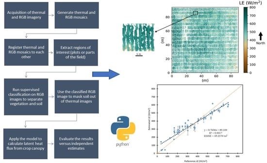
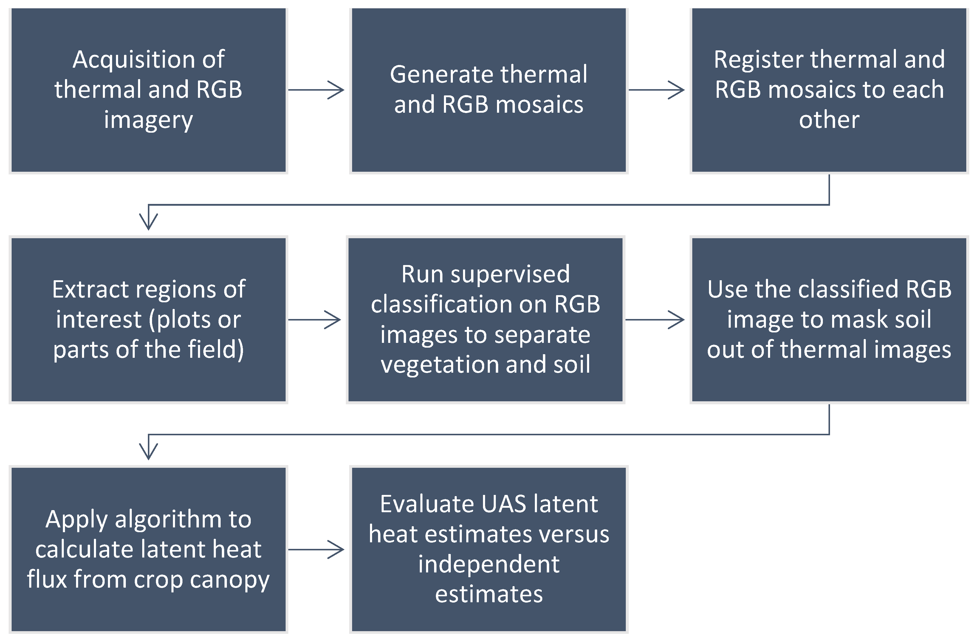
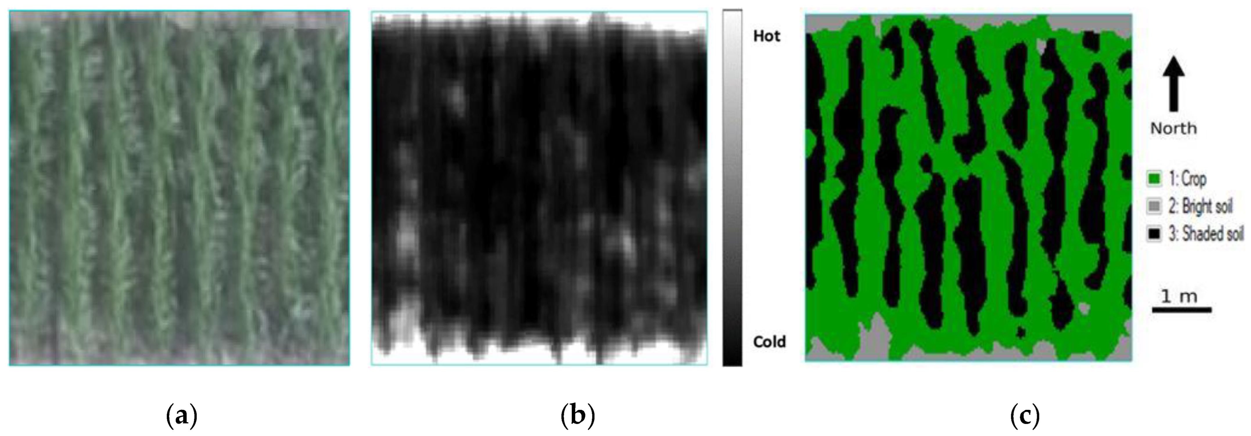
2.7. Image Analysis Workflow

The workflow for UAS-based latent heat flux calculations is summarized in Figure 3. After the acquisition of the imagery, a Pix4D mapper is used to generate mosaics for thermal and RGB images. The mosaics are then registered with each other in the ENVI software package (L3Harris Geospatial, CO, USA). Areas of interest which could be plots or the entire field are then extracted from the mosaics. Supervised classification is run on the RGB extractions to separate the canopy from soil and the resulting mask is applied to the corresponding thermal extractions to separate vegetation and soil. Only the pixels classified as vegetation are used for latent heat flux. Finally, results are evaluated versus independent measurements of latent heat flux.

3. Results

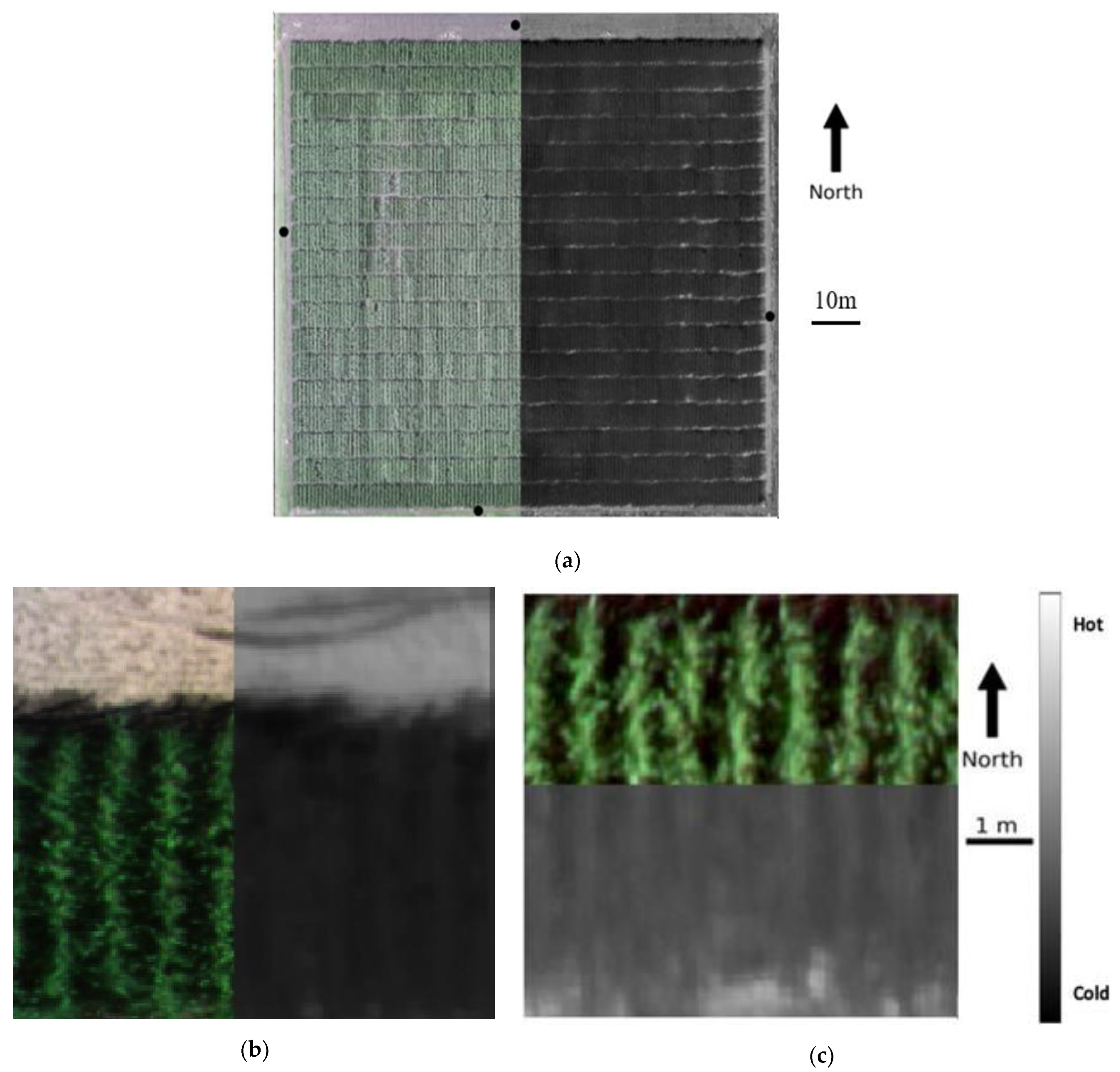
3.1. Image Registration Accuracy

Image registration and classification accuracy have also been evaluated on a sample dataset. Because of the lower resolution and limited contrast in the thermal infrared imagery, finding the ground control points deployed for georegistration around this field is difficult and their positions cannot be determined with the same degree of precision as in higher resolution imagery used on other flights. Four ground control points (GCPs) around the perimeter of the field (identified in Figure 4) are used to compute the RMSE of image coregistration between thermal and RGB imagery, and that of x (horizontal) direction is 0.019 m and that of y (vertical) direction is 0.028 m. Additionally, image registration can be evaluated through the visible inspection of image overlap as illustrated in Figure 4. From Figure 4, the individual segment and other ground features from both field level can be seen, and the plot level registration aligns well with each.

3.2. Canopy Classification Accuracy

In order to separate the vegetation from the soil, a supervised classification (Mahalanobis Distance, as described in Section 2.2) workflow was established in the ENVI software and applied to the RGB images. In order to demonstrate the accuracy of the classification scheme, Figure 5 presents an example of the classification results for one plot in F54N, and the classification accuracy results are summarized in Table 1.
The goal for this classification is to separate vegetation from soil pixels and only calculate the latent heat flux using those pixels identified as containing vegetation. While the method was applied to the entire experiment, results are demonstrated here using a single 8-row plot. In this example, there are three classes in the sample plot and the overall classification accuracy for all classes is above 96%. Also, the spectral features of both crop and shaded soil are similar, which results in the lower user accuracy for shaded soil.
To assess the sensitivity and specificity of the classification, the classes can be reduced to a binary choice: positive = crop, and negative = soil (sunlit and shaded), where the positive class is the class of interest. The sensitivity of the analysis is equal to the producer accuracy of the crop (95.45%), while the specificity is equal to the joint producer’s accuracy for the two soil classes (97.33%). This means that more than 95% of soil pixels are correctly classified as soil, while fewer than 3% of soil pixels are incorrectly classified as crop. As the experimental field is captured using the same RGB camera under similar illumination conditions and over a short period of time (typically less than 20 min), we assume that application of the same classification method to the whole field will result in a similar classification accuracy. The same classification methodology was applied to RGB images for all flight dates.

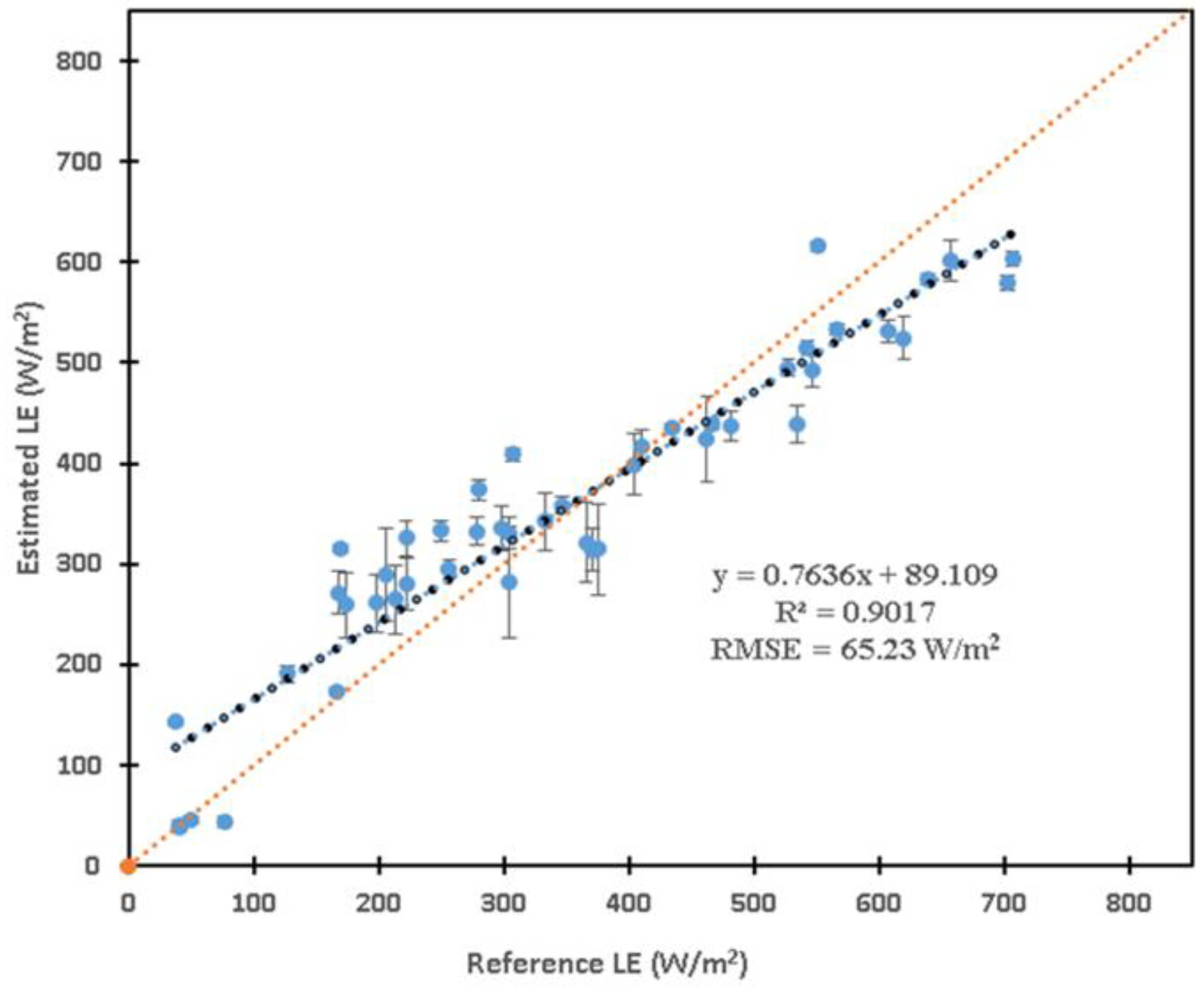
3.3. Evaluation of TSEB Model Latent Heat Estimates

Accurate canopy temperature measurements are critical for latent heat estimation. The RMSE of soil and canopy temperature extracted from the thermal imagery following the methods of Zhu et al. [24] was found to be less than 1.50 °C. The temperature accuracy of the calibrated images used for the flights presented here was confirmed to have a similar RMSE. The resulting temperature maps were then used to estimate latent heat for every canopy pixel on each flight date for both 2018 and 2020. Resulting latent heat flux estimates were evaluated for general responsiveness to climate conditions, and for accuracy versus porometry based latent heat estimates. The distribution of latent heat fluxes for each canopy pixel within the 8-row analysis plot for each flight date is presented in Figure 6.

3.3.1. Penmen-Monteith Based Latent Heat

The Penmen-Monteith (PM) equation was used to estimate the latent heat flux for the crop at the time of UAS flight operations using local weather observations summarized in Table 2. This results in a single value of LE for corn for the entire experiment, which can be compared against the distribution of LE that is calculated from the UAS imagery (Figure 6). This comparison was used to confirm that the TSEB estimates make sense relative to the weather conditions at the time of flight. For all dates in 2018 and 2020 included in the analysis, the Penmen-Monteith (PM) estimated latent heat is within the range of UAS estimated latent heat for the single plots where porometry measurements took place. PM latent heat values are well below the median UAS estimated LE for all observations between 60 and 80 days after planting (DAP), while late season estimates 31 August 2018 (DAP 115) and 28 August 2020 (DAP 108) fall between the median and first quartile line for both years. Overall, both the UAS and PM estimated latent heat fluxes respond as expected to the growth stage with latent heat increasing in the early season, stabilizing, then dropping late in the growing season. The effect of growth stage on latent heat is best illustrated by comparing observations with similar weather and growth stage between the years of observation, for example 12 July 2018 (DAP 65) with a median latent heat flux of 561.58 W/m2 and 14 July 2020 (DAP 63) of 556.47 W/m2 as well as 31 August 2018 (DAP 115) of 300.16 W/m2 and 28 August 2020 (DAP 108) of 292.11 W/m2.
Additional climate metrics are calculated (Table 2) and used to assess the role of real-time and antecedent environmental conditions on the estimated LE, with dates of special note described here in greater detail. The flight on 13 August 2020 (DAP 93) was especially late in the day (7:30 p.m.) when the reduced incoming solar radiation (109.40 W/m2) contributes to the closure of the stomata which results in the low latent heat flux (<100 W/m2). The five-day accumulated rain prior to the flight was also found to be helpful in understanding observed latent heat fluxes, for example, in July 2020, the incoming solar radiation is above 700 W/m2 for all dates, however, the accumulated rain prior to the 2 July (DAP 51) flight was only 2.03 mm which is significantly lower than the rest of dates, which results in its overall latent heat flux (median just under 400 W/m2) being amongst the lowest observed in July 2020.

3.3.2. Porometry Based Latent Heat

Porometer measurements of stomatal conductance were collected for a total of nine dates during the 2018 and 2020 field campaigns (Table 2) as described in Section 2. These measurements were used to estimate canopy transpiration, which in turn are compared with TSEB latent heat estimates for canopy pixels in the vicinity of the porometer measurements (Figure 7). The correlation between latent heat flux calculated from stomatal conductance measurements and that from the TSEB model is high, with an R2 higher than 0.90 and a low RMSE of 65.23 W/m2.
When latent heat flux is less than 400 W/m2, outputs from the UAS based model tend to overestimate the reference latent heat flux, while when the latent heat flux is over this threshold, outputs from the model underestimate the reference latent heat flux. The uncertainty of the model estimates is below 20 W/m2 for most of the measurements, which indicates that the temperature is relatively uniform across an area consisting of about 35 pixels. The variability of model estimates is smaller than that from the porometer measurements. This is most likely because the model assumes weather parameters (solar radiation, wind speed, air temperature, humidity, etc.) and plant phenotypic traits (plant height) are the same within an eight-row plot and the only variable is the vegetative temperature measured by the UAS camera. The ground reference measurements are subject to microclimate effects as well as to the actual measurement locations within the canopy.
The PM estimated latent heat flux values are generally lower than those estimated using the TSEB method. That is because of the need for standardization and to be able to quantify ET for most conditions, the constants in the PM equation presume a constant surface resistance of 70 s/m during all periods. This constant surface resistance which is equivalent to aerodynamic resistance in the TSEB model may cause some underprediction of hourly reference ET during some daytime periods when actual surface resistance may be somewhat lower [5].

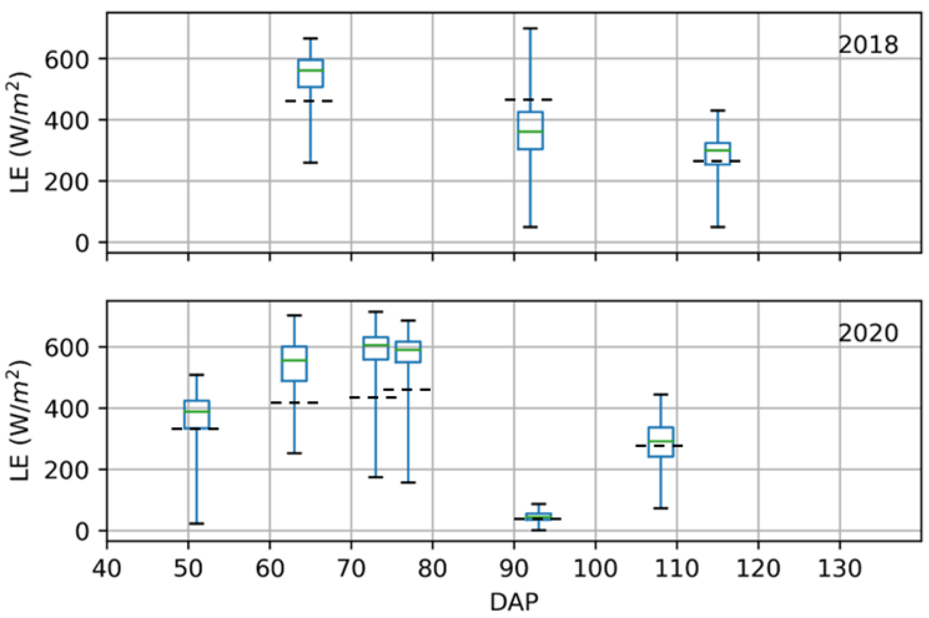
3.3.3. Change in Latent Heat through the Growing Season

The change in latent heat flux (shown in Figure 6) through the growing season can also be visualized by looking at the spatial distribution of latent heat estimated at the plot scale (Figure 8). There is some increase in canopy closure through the first four dates in 2020, but the latent heat is estimated only for the leaf area, so the change in latent heat between days should be independent of the canopy area. As noted previously, the solar radiation between the first four measurement dates in 2020 (Figure 8a–d) is very similar (between 705 and 744 W/m2) but latent heat flux is low on 2 July (DAP 51; Figure 8a). In this case, most of the other environmental factors are similar, the biggest difference is the total rainfall over the previous five days, which was very low (2.03 mm) compared to the next three days, which had precipitation totals of 27.69, 15.49 and 34.04 mm, respectively. This suggests that the target plot was under greater water stress on the first date of observation than on the subsequent ones.
Measurements on 13 August 2020 (Figure 8e) are later in the growing season, but not late enough that a substantial drop in latent heat flux would be expected. Air temperature, wind speed and rainfall are comparable with other sampling dates. The humidity is higher and the incoming solar radiation is lower than all other observation dates. While the higher humidity likely helps constrain latent heat, the bigger factor is the reduced solar radiation. Flights on that day occurred much later in the day, at 7:30 p.m. local time, and latent heat is severely limited by the incoming solar radiation that is only 109.4 W/m2.
The final flight date of the 2020 season on 28 August (DAP 108) also found consistently low latent heat flux across the plot (Figure 8f). Flight time is again in-line with the earlier dates, as are temperature, wind speed and antecedent precipitation. Humidity is still higher, while solar radiation is still lower than that found in the July flights. Lower latent heat estimates are consistent with the lower solar radiation, but the crop is also nearing senescence, which would also reduce latent heat.
It can also be seen from Table 2 that the range of RMSE is from 16.76 to 106.63 W/m2. The lowest RMSE appear on 13 August 2020 when there is low solar radiation and low latent heat flux in general; the highest RMSE, however, happened on 28 July 2020 when the latent heat flux is one of the highest among all dates in 2020. This is in agreementwith the findings in Figure 7, which indicate that the largest errors occur when the reference latent heat flux is low or high. On 2 July 2020, since there was a water deficit stress, the soil temperature was consistently higher than the canopy temperature measured. That is visualized in the Figure 8a in which the northern and southern parts of the vegetative plots have obviously lower latent heat flux compared with the other parts of the plots. That is because the soil of high temperature emits radiation that heats the leaves. Leaves of high temperature are considered to have less latent heat flux.

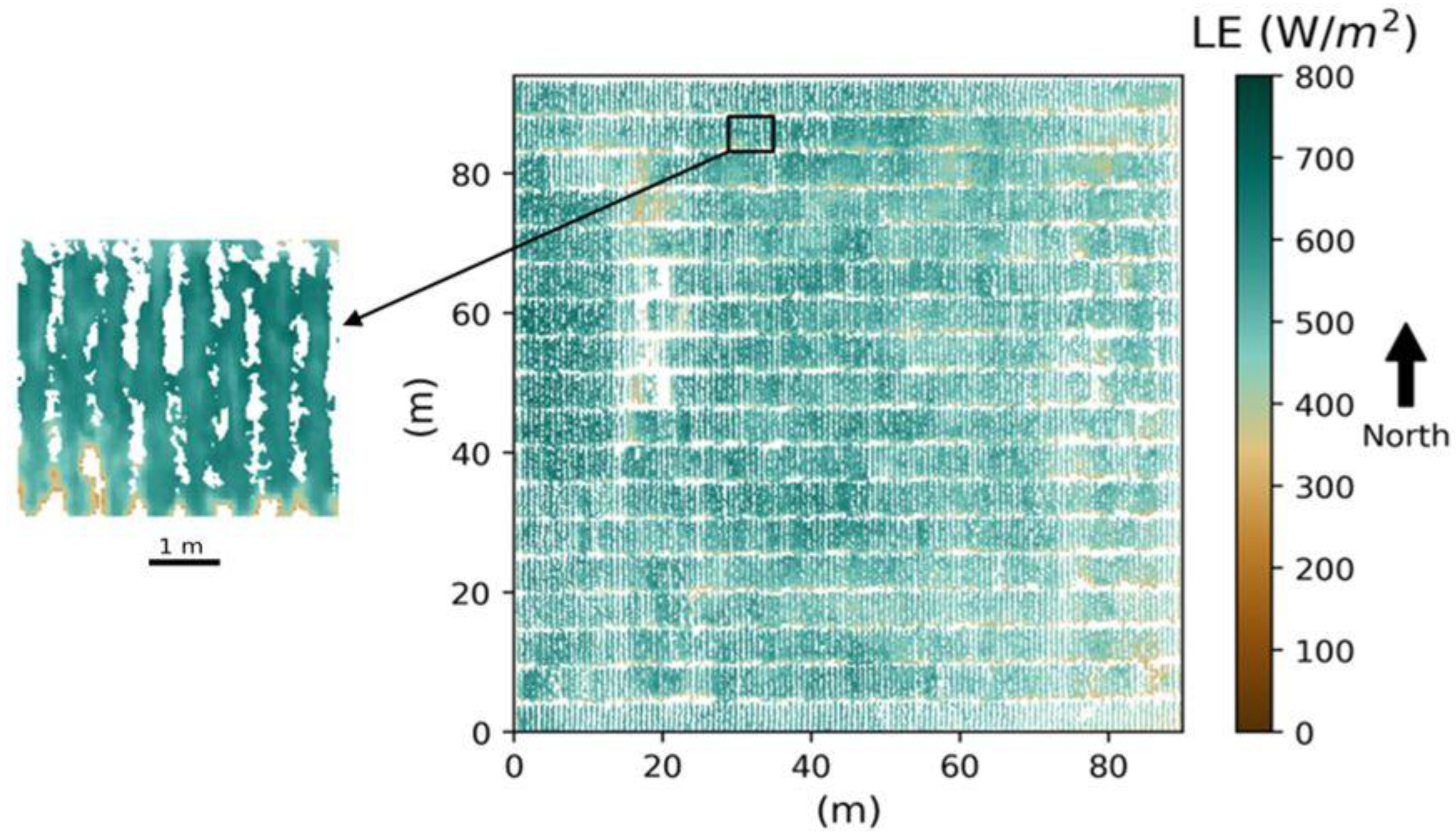
3.3.4. Latent Heat Flux of the Entire Field

A latent heat flux map of an entire field (Figure 9) has been generated to demonstrate the ability of the workflow to provide information at a larger scale. This map shows that for a large part of the field, the latent heat flux is above 400 W/m2, with the lowest latent heat fluxes concentrated at the ends of field plots. The area around 20 m east and 50 m north is mostly devoid of latent heat flux estimates because the crops in this area are not well developed. The area of relatively consistent high latent heat between 0 and 15 m east and 40 to 80 m north is a single experiment with more consistent genetics. The full field is subdivided into three breeding experiments in the east, middle and west parts of the field with border rows of a commercial variety (same genetics) between them and between the experiments and the field edges. The central experiment is also visible as an area with more consistent high latent heat flux. In general, the field on this day is not under water stress, which is consistent with the weather conditions listed in Table 2. The plot identified in the figure is the same plot as in Figure 8d.

4. Discussion

Efficient use of water resources has become increasingly important because of rapid depletion, industrial development, population increase, more frequent drought conditions, and degradation of ground and surface water quality in many regions [39]. Improved techniques are needed for accurate quantification of latent heat flux at the field or plot scale to facilitate irrigation management and to provide additional information on susceptibility to water stress in crop breeding experiments. Satellite and aircraft based remote sensing platforms with thermal infrared sensors have been used for quantifying the water status of crops for many years, but interest has been growing in recent years with the increased availability of inexpensive thermal infrared cameras mounted on UAS platforms. Obtaining accurate canopy and soil temperature measurements from such systems was addressed in Zhu et al. [24], while this research focuses on the estimation of latent heat flux from the crop canopy using thermal infrared imagery and local weather observations. Traditional workflows for latent heat estimation were designed for coarser resolution datasets collected from satellite or aircraft systems that cannot distinguish between vegetation and soil. Latent heat estimation methods from such datasets must deal with errors and uncertainty introduced into the latent heat estimates from the mixture of soil and vegetation in the remote sensing imagery. This study presents a novel workflow for crop latent heat flux quantification from high-resolution (around 5 cm per pixel) imagery, in which RGB imagery was used to distinguish between vegetation and soil by supervised classification and then was used to mask thermal imagery so that only canopy pixels were included in the latent heat calculations. As with the two-source energy balance (TSEB) model on which it is based, the method made use of two atmospheric stability scenarios where the relative temperature of the canopy to the air was used to determine if conditions were stable and unstable, which affects the estimation of latent heat flux.
Penmen-Monteith (PM) estimated latent heat is within the range of UAS estimated latent heat for the single plots where porometry measurements took place. Overall, both the UAS and PM estimated latent heat fluxes respond as expected to the crop growth stage with latent heat increasing in the early season, stabilizing, then dropping late in the growing season. The effect of growth stage on latent heat is best illustrated by comparing observations with similar weather and growth stages between the years of observation. The effect of changing weather conditions can also be observed in the UAS-estimated latent heat flux by comparisons between crops in similar growth stages but with different weather conditions. Latent heat fluxes did respond as expected to changes in weather conditions quantified using metrics such as total rainfall over the previous five days and relative humidity. This indicates that the UAS-based latent heat estimates have potential for monitoring crop water stress.
For latent heat flux estimation from the TSEB model, Brenner et al. [18] reported an RMSE of 69 W/m2, which is higher than the RMSE reported here. Riveros-Burgos et al. [21] reported an RMSE value of 37 W/m2 for latent heat flux estimations using a clumped model to directly estimate LE over discontinuous canopies in an olive orchard. However, the flight’s starting time varied from 12:39 to 14:17 and the LE range is from 100 to 220 W/m2, which may increase the estimation accuracy because only low latent heat flux conditions were considered.
Similarly, Ortega-Farías et al. [20] reported that the RMSE value for LE is 50 W/m2 using an energy balance algorithm over a drip-irrigated olive orchard. The flight time is constrained between 11:56 a.m. to 12:46 p.m. local time and the incoming solar radiation is from 801 to 901 W/m2.
Nieto et al. [23] used four different TSEB approaches to estimate the component soil and canopy temperatures and ET partitioning between soil and canopy. Thirteen data acquisition flights were conducted from 2014 to 2016. They were using an empirical NDVI threshold to differentiate between canopy and soil to retrieve soil and canopy temperatures separately. The pixel resolution for their visible and near-infrared datasets are 0.15 m and 0.6 m, respectively. They estimated that the RMSE range of latent heat flux estimates is from 49 to 75 W/m2 for the four approaches used in their research.
The accuracy reported here is sufficient to estimate the instantaneous latent heat flux with an average of RMSE of 65.23 W/m2, which is within the range achieved by other researchers. Challenges remain for the testing of the algorithm for more types of crops and a variety of atmospheric conditions. Also, the latent heat flux acquired here is on a pixel level, so how to reduce the information to provide a value for a plant and a plot accurately will need to be investigated in the future.

5. Conclusions

A workflow was presented to estimate the latent heat flux of row crops from a UAS-based thermal and RGB camera system. The main part of the workflow is to use a modified TSEB model to calculate the values of canopy latent heat on a pixel level. The workflow developed here requires high resolution RGB and thermal imagery from a single camera and a variety of weather parameters collected locally. The RGB data is classified into canopy and soil and used to mask the thermal imagery to extract canopy temperatures that are then used to calculate latent heat flux from a field experiment with corn being planted.
The latent heat estimates are evaluated against ground reference measurements using both in-situ porometer measurements and calculating latent heat using the Penmen-Monteith method using local weather conditions. When comparing with the ground reference data calculated from porometer measurements, the RMSE for between latent heat estimated using UAS imagery and porometer surveys for nine flight dates in 2018 and 2020 is 65.23 W/m2, with a coefficient of determination (R2) that is above 0.9. The results indicate that the workflow developed here is suitable for using high resolution thermal imagery to calculate the latent heat flux of corn accurately.
The best estimation results usually were achieved in cloudless weather conditions when solar radiation did not change abruptly. When there were intense clouds in the sky, solar radiation could change dramatically, which brought huge errors to the estimation results. However, through the calibrations, reasonable results were able to be achieved under a variety of weather and illumination conditions.
Future work includes testing the performance of this workflow on more types of crops and also the development of an appropriate way to account for the variance of latent heat flux on different parts of leaves, for example differences in LE estimation from sunlit and shaded leaves, even on the same plant.

Author Contributions

Conceptualization, Y.Z. and K.A.C.; methodology, Y.Z. and K.A.C.; writing—review and editing, Y.Z., K.A.C. and E.M.L.; funding acquisition, K.A.C. All authors have read and agreed to the published version of the manuscript.

Funding

This research was funded in part by the Advanced Research Projects Agency-Energy (ARPA-E) of the U.S. Department of Energy under Award No. DE-AR0001135.

Acknowledgments

We thank John Evan Flatt, John Bullock, Lucas Wright and Nicholas Hansen for piloting the UAS and in helping deploy the water targets in the field.

Conflicts of Interest

The other authors declare that they have no conflict of interest. Keith A. Cherkauer is a founder of and owns stock in GRYFN.

References

  1. Jensen, M.E.; Allen, R.G. Evaporation, Evapotranspiration, and Irrigation Water Requirements, 2nd ed.; American Society of Civil Engineers: Reston, VA, USA, 2016. [Google Scholar] [CrossRef]
  2. Anderson, M.C.; Allen, R.G.; Morse, A.; Kustas, W.P. Use of Landsat Thermal Imagery in Monitoring Evapotranspiration and Managing Water Resources. Remote Sens. Environ. 2012, 122, 50–65. [Google Scholar] [CrossRef]
  3. Khanal, S.; Fulton, J.; Shearer, S. An Overview of Current and Potential Applications of Thermal Remote Sensing in Precision Agriculture. Comput. Electron. Agric. 2017, 139, 22–32. [Google Scholar] [CrossRef]
  4. Zhu, Y.; Cherkauer, K. Estimation of Crop Latent Heat Flux from High Resolution Thermal Imagery. In Proceedings of the Autonomous Air and Ground Sensing Systems for Agricultural Optimization and Phenotyping IV, Baltimore, MD, USA, 14 May 2019. [Google Scholar] [CrossRef]
  5. Allen, R.G. Crop Evapotranspiration: Guidelines for Computing Crop Water Requirements; Food and Agriculture Organization of the United Nations, Ed.; FAO Irrigation and Drainage Paper; Food and Agriculture Organization of the United Nations: Rome, Italy, 1998; ISBN 978-92-5-104219-9. [Google Scholar]
  6. Heitman, J.L.; Horton, R.; Sauer, T.J.; Ren, T.S.; Xiao, X. Latent Heat in Soil Heat Flux Measurements. Agric. For. Meteorol. 2010, 150, 1147–1153. [Google Scholar] [CrossRef] [Green Version]
  7. Marek, T.H.; Schneider, A.D.; Howell, T.A.; Ebeling, L.L. Design and Construction of Large Weighing Monolithic Lysimeters. Trans. ASAE 1988, 31, 0477–0484. [Google Scholar] [CrossRef]
  8. Howell, T.A.; McCormick, R.L.; Phene, C.J. Design and Installation of Large Weighing Lysimeters. Trans. ASAE 1985, 28, 106–112. [Google Scholar] [CrossRef]
  9. Swinbank, W.C. The measurement of vertical transfer of heat and water vapor by eddies in the lower atmosphere. J. Meteorol. 1951, 8, 135–145. [Google Scholar] [CrossRef] [Green Version]
  10. Twine, T.E.; Kustas, W.P.; Norman, J.M.; Cook, D.R.; Houser, P.R.; Meyers, T.P.; Prueger, J.H.; Starks, P.J.; Wesely, M.L. Correcting Eddy-Covariance Flux Underestimates over a Grassland. Agric. For. Meteorol. 2000, 103, 279–300. [Google Scholar] [CrossRef] [Green Version]
  11. Bowen, I.S. The Ratio of Heat Losses by Conduction and by Evaporation from Any Water Surface. Phys. Rev. 1926, 27, 779–787. [Google Scholar] [CrossRef] [Green Version]
  12. Penman, H.L. Natural Evaporation from Open Water, Bare Soil and Grass. Proc. R. Soc. Lond. Ser. A Math. Phys. Sci. 1948, 193, 120–145. [Google Scholar] [CrossRef] [Green Version]
  13. Singh, R.K.; Irmak, A. Estimation of Crop Coefficients Using Satellite Remote Sensing. J. Irrig. Drain. Eng. 2009, 135, 597–608. [Google Scholar] [CrossRef]
  14. Song, L.; Liu, S.; Kustas, W.P.; Zhou, J.; Xu, Z.; Xia, T.; Li, M. Application of Remote Sensing-Based Two-Source Energy Balance Model for Mapping Field Surface Fluxes with Composite and Component Surface Temperatures. Agric. For. Meteorol. 2016, 230–231, 8–19. [Google Scholar] [CrossRef] [Green Version]
  15. Hoffmann, H.; Nieto, H.; Jensen, R.; Guzinski, R.; Zarco-Tejada, P.; Friborg, T. Estimating Evaporation with Thermal UAV Data and Two-Source Energy Balance Models. Hydrol. Earth Syst. Sci. 2016, 20, 697–713. [Google Scholar] [CrossRef] [Green Version]
  16. Norman, J.M.; Kustas, W.P.; Humes, K.S. Source Approach for Estimating Soil and Vegetation Energy Fluxes in Observations of Directional Radiometric Surface Temperature. Agric. For. Meteorol. 1995, 77, 263–293. [Google Scholar] [CrossRef]
  17. Priestley, C.H.B.; Taylor, R.J. On the Assessment of Surface Heat Flux and Evaporation Using Large-Scale Parameters. Mon. Weather Rev. 1972, 100, 81–92. [Google Scholar] [CrossRef]
  18. Brenner, C.; Thiem, C.E.; Wizemann, H.-D.; Bernhardt, M.; Schulz, K. Estimating Spatially Distributed Turbulent Heat Fluxes from High-Resolution Thermal Imagery Acquired with a UAV System. Int. J. Remote Sens. 2017, 38, 3003–3026. [Google Scholar] [CrossRef] [Green Version]
  19. Norman, J.M.; Kustas, W.P.; Prueger, J.H.; Diak, G.R. Surface Flux Estimation Using Radiometric Temperature: A Dual-Temperature-Difference Method to Minimize Measurement Errors. Water Resour. Res. 2000, 36, 2263–2274. [Google Scholar] [CrossRef] [Green Version]
  20. Ortega-Farías, S.; Ortega-Salazar, S.; Poblete, T.; Kilic, A.; Allen, R.; Poblete-Echeverría, C.; Ahumada-Orellana, L.; Zuñiga, M.; Sepúlveda, D. Estimation of Energy Balance Components over a Drip-Irrigated Olive Orchard Using Thermal and Multispectral Cameras Placed on a Helicopter-Based Unmanned Aerial Vehicle (UAV). Remote Sens. 2016, 8, 638. [Google Scholar] [CrossRef] [Green Version]
  21. Riveros-Burgos, C.; Ortega-Farías, S.; Morales-Salinas, L.; Fuentes-Peñailillo, F.; Tian, F. Assessment of the Clumped Model to Estimate Olive Orchard Evapotranspiration Using Meteorological Data and UAV-Based Thermal Infrared Imagery. Irrig. Sci. 2021, 39, 63–80. [Google Scholar] [CrossRef]
  22. Brenner, A.J.; Incoll, L.D. The Effect of Clumping and Stomatal Response on Evaporation from Sparsely Vegetated Shrublands. Agric. For. Meteorol. 1997, 84, 187–205. [Google Scholar] [CrossRef]
  23. Nieto, H.; Kustas, W.P.; Torres-Rúa, A.; Alfieri, J.G.; Gao, F.; Anderson, M.C.; White, W.A.; Song, L.; del Mar Alsina, M.; Prueger, J.H.; et al. Evaluation of TSEB Turbulent Fluxes Using Different Methods for the Retrieval of Soil and Canopy Component Temperatures from UAV Thermal and Multispectral Imagery. Irrig. Sci. 2019, 37, 389–406. [Google Scholar] [CrossRef] [Green Version]
  24. Zhu, Y.; Cherkauer, K. Pixel-Based Calibration and Atmospheric Correction of a UAS-Mounted Thermal Camera for Land Surface Temperature Measurements. Trans. ASABE 2021, 64, 2137–2150. [Google Scholar] [CrossRef]
  25. De Maesschalck, R.; Jouan-Rimbaud, D.; Massart, D.L. The Mahalanobis Distance. Chemom. Intell. Lab. Syst. 2000, 50, 1–18. [Google Scholar] [CrossRef]
  26. Lillesand, T.M.; Kiefer, R.W.; Chipman, J.W. Remote Sensing and Image Interpretation, 7th ed.; John Wiley & Sons, Inc.: Hoboken, NJ, USA, 2015; ISBN 978-1-118-34328-9. [Google Scholar]
  27. Colaizzi, P.D.; Kustas, W.P.; Anderson, M.C.; Agam, N.; Tolk, J.A.; Evett, S.R.; Howell, T.A.; Gowda, P.H.; O’Shaughnessy, S.A. Two-Source Energy Balance Model Estimates of Evapotranspiration Using Component and Composite Surface Temperatures. Adv. Water Resour. 2012, 50, 134–151. [Google Scholar] [CrossRef] [Green Version]
  28. Tang, R.; Li, Z.-L.; Jia, Y.; Li, C.; Chen, K.-S.; Sun, X.; Lou, J. Evaluating One- and Two-Source Energy Balance Models in Estimating Surface Evapotranspiration from Landsat-Derived Surface Temperature and Field Measurements. Int. J. Remote Sens. 2013, 34, 3299–3313. [Google Scholar] [CrossRef]
  29. Kustas, W.P.; Norman, J.M. Evaluation of Soil and Vegetation Heat Flux Predictions Using a Simple Two-Source Model with Radiometric Temperatures for Partial Canopy Cover. Agric. For. Meteorol. 1999, 94, 13–29. [Google Scholar] [CrossRef]
  30. Campbell, G.S.; Norman, J.M. An Introduction to Environmental Biophysics; Springer: New York, NY, USA, 1998; ISBN 978-0-387-94937-6. [Google Scholar]
  31. Weiss, A.; Norman, J.M. Partitioning Solar Radiation into Direct and Diffuse, Visible and near-Infrared Components. Agric. For. Meteorol. 1985, 34, 205–213. [Google Scholar] [CrossRef]
  32. Monin, A.S.; Obukhov, A.M. Basic Laws of Turbulent Mixing in the Surface Layer of the Atmosphere. Contrib. Geophys. Inst. Acad. Sci. USSR 1954, 151, e187. [Google Scholar]
  33. Brutsaert, W. Hydrology: An Introduction; Cambridge University Press: Cambridge, UK; New York, NY, USA, 2005; ISBN 978-0-521-82479-8. [Google Scholar]
  34. Piccinni, G.; Ko, J.; Marek, T.; Howell, T. Determination of Growth-Stage-Specific Crop Coefficients (KC) of Maize and Sorghum. Agric. Water Manag. 2009, 96, 1698–1704. [Google Scholar] [CrossRef]
  35. SC-1. Available online: http://library.metergroup.com/Manuals/20773%20_SC-1_Manual_Web.pdf (accessed on 5 January 2022).
  36. Jackson, R.D.; Idso, S.B.; Reginato, R.J.; Pinter, P.J. Canopy Temperature as a Crop Water Stress Indicator. Water Resour. Res. 1981, 17, 1133–1138. [Google Scholar] [CrossRef]
  37. Gerosa, G.; Mereu, S.; Finco, A.; Marzuoli, R. Stomatal Conductance Modeling to Estimate the Evapotranspiration of Natural and Agricultural Ecosystems. In Evapotranspiration-Remote Sensing and Modeling; Irmak, A., Ed.; InTech: London, UK, 2012; ISBN 978-953-307-808-3. [Google Scholar]
  38. Zhu, Y.; Irmak, S.; Jhala, A.J.; Vuran, M.C.; Diotto, A. Time-Domain and Frequency-Domain Reflectometry Type Soil Moisture Sensor Performance and Soil Temperature Effects in Fine- and Coarse-Textured Soils. Appl. Eng. Agric. 2019, 35, 117–134. [Google Scholar] [CrossRef]
  39. Irmak, S. Evapotranspiration. In Encyclopedia of Ecology; Elsevier: Amsterdam, The Netherlands, 2008; pp. 1432–1438. ISBN 978-0-08-045405-4. [Google Scholar]
Figure 1. Locations of ACRE and the research field (image acquired from Google Maps).
Remotesensing 14 02682 g001
Figure 2. Ground reference measurements in F54 north on 28 August 2020 (a) stomatal conductance measurements from SC-1 leaf porometer; (b) LAI measurements from LAI-2200C plant canopy analyzer.
Remotesensing 14 02682 g002
Figure 3. Latent heat flux calculations workflow.
Remotesensing 14 02682 g003
Figure 4. Comparison of the registration between RGB and thermal infrared images (stretched for better visualization) taken on 28 July 2020. Both images were collected at the same time from the same camera during flight, but have slightly different fields of view and resolutions, so co-registration is required to remove any offsets. (a) field level registration where black dots indicate the GCPs used for registration accuracy evaluation; (b) plot level registration (vertical registration); (c) plot level registration (horizontal registration).
Remotesensing 14 02682 g004
Figure 5. Supervised classification result of a plot in F54 north on 28 July 2020. (a) original RGB image; (b) thermal image (stretched for better visualization); (c) supervised classification result based on the RGB image.
Remotesensing 14 02682 g005
Figure 6. Box plots of latent heat flux distribution estimated from UAS imagery within the sample area of target plots in Field 54 north, where the black dashed lines indicate the latent heat flux values calculated from the Penman-Monteith equation for the time of observation and top whisker indicates the highest LE values, the top of the box indicates the 25th percentile LE, the middle line indicates the median LE, the bottom of the box indicates that 75th percentile LE, and the lower whisker indicates the lowest values of LE. The x-axis is labeled based on the days after planting (DAP), which is specific to the year and field being evaluated.
Remotesensing 14 02682 g006
Figure 7. Scatter plot of reference latent heat flux calculated using porometer measurements versus TSEB model estimations. Symbol indicates the average value of measurements, while the error bars indicate the standard deviation of model estimates based on all pixels identified as potentially representing the location of the porometer measurements. Data is for all days of flight operations in 2018 and 2020.
Remotesensing 14 02682 g007
Figure 8. Latent heat flux estimates for the target plot in F54 north of six different dates. (a) 2 July 2020 (DAP 51); (b) 14 July 2020 (DAP 63); (c) 24 July 2020 (DAP 73); (d) 28 July 2020 (DAP 77); (e) 13 August 2020 (DAP 93); (f) 28 August 2020 (DAP 108). Images are clipped so latent heat flux is estimated only for canopy pixels.
Remotesensing 14 02682 g008
Figure 9. Latent heat flux map of field 54 north on 28 July 2020 with a zoomed in picture showing the plot in detail.
Remotesensing 14 02682 g009
Table 1. Classification results. Confusion matrix for classification evaluation including producer and user accuracy of three classes: Crop, Sunlit Soil and Shaded Soil is of a plot in F54N on 28 July 2020.
Ground Reference
ClassCropSunlit SoilShaded SoilRow
Total
User Accuracy
Crop1070210998.17%
PredictedSunlit Soil13003196.77%
Shaded Soil40434791.49%
Column Total1123045187
Producer
Accuracy
95.54%100.00%95.56% Overall Accuracy
96.26%
Table 2. Weather parameters on the day of flight operations including those used to estimate latent heat (air temperature, wind speed, relative humidity and solar radiation), used to assess crop growth stage and water stress (five-day rain accumulation and days after planting (DAP)) and the RMSE of latent heat estimated from UAS imagery versus the porometry measurements. Date and time of each flight in 2018 and 2020 is provided. Air temperature, wind speed, relative humidity and solar radiation are from the 30-min period including the flight, while the five-day rain accumulation is for the five-day period preceding each flight operation.
TimeAir
Temperature (°C)
Wind Speed (m/s)Relative Humidity (%)Solar
Radiation (W/m2)
5-Day Rain (mm)DAPRMSE
(W/m2)
12 July 2018(16:00)29.52.144.7836.9410.166569.37
8 August 2018
(15:30)
28.54.757.7699.1724.139263.03
31 August 2018
(17:00)
31.13.056.5459.589.1411560.99
2 July 2020
(17:00)
31.13.640.9705.002.035171.82
14 July 2020
(16:30)
29.04.043.5743.6527.696354.52
24 July 2020
(17:00)
28.92.249.1731.6415.497370.08
28 July 2020
(17:00)
28.83.146.2707.9034.0477106.63
13 August 2020
(19:30)
26.62.764.5109.4020.329316.76
28 August 2020
(16:30)
30.73.160.0568.305.8410865.02
Publisher’s Note: MDPI stays neutral with regard to jurisdictional claims in published maps and institutional affiliations.

