
Integrating Deep Learning and Hydrodynamic Modeling to Improve the Great Lakes Forecast
by
 , and
, and
Pengfei Xue
1,2,3,4,* ,
,
Aditya Wagh
5,
Gangfeng Ma
6,
Yilin Wang
7,
Yongchao Yang
5,
Tao Liu
8 and
and
Chenfu Huang
2 1
Department of Civil, Environmental and Geospatial Engineering, Michigan Technological University, Houghton, MI 49931, USA
2
Great Lakes Research Center, Michigan Technological University, Houghton, MI 49931, USA
3
Argonne National Laboratory, Environmental Science Division, Lemont, IL 60439, USA
4
Department of Civil and Environmental Engineering, Massachusetts Institute of Technology, Cambridge, MA 02139, USA
5
Department of Mechanical Engineering-Engineering Mechanics, Michigan Technological University, Houghton, MI 49931, USA
6
Department of Civil and Environmental Engineering, Old Dominion University, Norfolk, VA 23529, USA
7
Department of Computer Science, Michigan Technological University, Houghton, MI 49931, USA
8
College of Forest Resources and Environmental Science, Michigan Technological University, Houghton, MI 49931, USA
*
Author to whom correspondence should be addressed.
Remote Sens. 2022, 14(11), 2640; https://doi.org/10.3390/rs14112640
Submission received: 16 April 2022
/
Revised: 22 May 2022
/
Accepted: 27 May 2022
/
Published: 31 May 2022
(This article belongs to the Special Issue Linking Upper Ocean Dynamics with Extreme Weather and Climate Events over the Ocean)
Abstract
:The Laurentian Great Lakes, one of the world’s largest surface freshwater systems, pose a modeling challenge in seasonal forecast and climate projection. While physics-based hydrodynamic modeling is a fundamental approach, improving the forecast accuracy remains critical. In recent years, machine learning (ML) has quickly emerged in geoscience applications, but its application to the Great Lakes hydrodynamic prediction is still in its early stages. This work is the first one to explore a deep learning approach to predicting spatiotemporal distributions of the lake surface temperature (LST) in the Great Lakes. Our study shows that the Long Short-Term Memory (LSTM) neural network, trained with the limited data from hypothetical monitoring networks, can provide consistent and robust performance. The LSTM prediction captured the LST spatiotemporal variabilities across the five Great Lakes well, suggesting an effective and efficient way for monitoring network design in assisting the ML-based forecast. Furthermore, we employed an explainable artificial intelligence (XAI) technique named SHapley Additive exPlanations (SHAP) to uncover how the features impact the LSTM prediction. Our XAI analysis shows air temperature is the most influential feature for predicting LST in the trained LSTM. The relatively large bias in the LSTM prediction during the spring and fall was associated with substantial heterogeneity of air temperature during the two seasons. In contrast, the physics-based hydrodynamic model performed better in spring and fall yet exhibited relatively large biases during the summer stratification period. Finally, we developed a statistical integration of the hydrodynamic modeling and deep learning results based on the Best Linear Unbiased Estimator (BLUE). The integration further enhanced prediction accuracy, suggesting its potential for next-generation Great Lakes forecast systems.
Keywords:
deep learning; LSTM; XAI; lake surface temperature; Great Lakes; model integration; earth system1. Introduction
The Laurentian Great Lakes, including Lake Superior, Lake Michigan, Lake Huron, Lake Ontario, and Lake Erie, are the world’s largest freshwater systems. The five lakes collectively contain 84% of North America’s surface fresh water and 21% of Earth’s surface fresh water [1]. With a maximum water depth of more than 400 m and spanning a region of 94,250 square miles (approximately 2.6 times greater than the Gulf of Maine), the vast freshwater system has long been referred to as “inland seas”. They exhibit sea-like characteristics such as basin-wide gyres, coastal jet currents, regional upwellings, thermal bars, rolling waves, and large thermal and ice variability.
Due to their large volume and surface area, the Great Lakes are a significant driver of regional weather and climate. Lake surface temperature (LST) is a fundamental thermodynamic variable for the regional climate [2,3,4,5], and a widely used environmental indicator for climate and environmental changes [6,7,8,9]. LST, as an over-lake lower boundary condition for atmospheric processes, influences the climate and hydroclimate through various multiscale lake–atmosphere interactions [4,5,10]. Large lake thermal inertia reduces annual and diurnal temperature variability across the Great Lakes basin [11] and results in a less significant warming over the lakes than over the surrounding land [10]. LST also has a strong influence on regional precipitation patterns. During cold seasons, as the cold air mass travels over the unfrozen and relatively warm waters of the Great Lakes, LST is a key factor in determining moisture and heat supplies from the lake, which leads to the formation of lake-effect snow on the lee sides of the Great Lakes [2,4]. During warm seasons, higher LST increases local instability and enhances moisture transport, which alternates the regional precipitation pattern by reducing mesoscale convective precipitation upstream of the Great Lakes region and increasing isolated deep convective precipitation and non-convective precipitation downstream of the Great Lakes region [5]. Therefore, an accurate estimation of LST is not only crucial for lake hydrodynamic processes it is also critical for understanding regional climate change and weather extremes.
LST in the Great Lakes exhibits strong seasonal, interannual, and spatial variabilities. The LST ranges from 0 °C during the winter to more than 30 °C during the summer. The summer temperature can vary more than 10–15 °C between cold and warm years and across the lakes. The strong variability of LST is controlled by regional meteorological processes through their impacts on lake surface heat and momentum fluxes [12,13], as well as hydrodynamic processes such as stratifications, overturns, gyres, upwellings, river plumes, and the presence of ice in the winter [8,14,15,16,17].
Physics-based hydrodynamic modeling is a common and fundamental approach to predicting lake conditions. It simulates a set of spatiotemporally varying state variables to predict hydrodynamic conditions, using the numerical integration of the governing equations [18]. However, due to uncertainties in model representation of physical processes, boundary forcing, and parameterization, modeling errors still exist in hydrodynamic simulations [8,17,19,20]. Various efforts have been made to improve the Great Lakes hydrodynamic modeling, such as improving the representation of the physical processes [21,22], resolving the interactions of the atmosphere–lake interface [3,10,23], improving model resolution and forcing accuracy [13,22], and incorporating data assimilation techniques [8]. While significant advancements have been made for the Great Lakes hydrodynamic modeling, improving the forecast accuracy remains critical.
Machine learning (ML) has quickly emerged in geoscience applications as a new technology to improve hydrodynamic forecasting. Examples include applying deep learning neural networks to a postprocessing framework to improve atmospheric river forecasts [24], developing an emulator of the simplified general circulation models [25,26], detecting extreme events from large climate datasets [27], predicting weather forecast uncertainties [28], building a hybrid model to conserve the surface energy balance [29], approximating the subgrid-scale processes in climate modeling [30], determining the weighted aggregation to combine ensemble wave forecasts [31,32], correcting the cold bias of sea surface temperature to improve the typhoon–ocean feedback [33,34], and predicting unresolved turbulent processes and subsurface flow fields to leverage observations and coarse-resolution model data [35].
However, the ML application to the Great Lakes is still in its early stages. Until recently, deep learning has begun to be used for the Great Lakes hydrodynamic modeling, in particular, in wave simulation in Lake Erie and Lake Michigan [36,37]. Hu et al. [37] tested two ML approaches for predicting wave height and period at two selected buoy locations in Lake Erie, based on the local wind information. The results show that both ML techniques improved the prediction of wave height spikes under strong wind conditions compared to a physics-based wave model (WaveWatch III). Nonetheless, their predictions were limited to two observational locations and does not provide wave conditions for the entire Lake Erie. On the other hand, Feng et al. [36] applied a multi-layer perceptron (MLP) network for wave prediction in Lake Michigan. The MLP was trained using the data generated by a physics-based SWAN (Simulating WAves Nearshore) model for 2005–2014 and tested for wave prediction in 2015 for the entire Lake Michigan. Hence, the MLP performance depended on the SWAN model accuracy. Their research focused on using deep learning as an emulator of the SWAN to improve computational efficiency.
Applying deep learning to the LST prediction makes the situation more challenging. Unlike waves that are primarily controlled by wind features, the LST is influenced by various meteorological factors such as surface air temperature, wind, surface heat fluxes, as well as lake thermodynamics and hydrodynamics. This paper explores the feasibility of using deep learning techniques to predict LSTs in all five Great Lakes under a scenario when only limited observational data are available. Furthermore, we apply an explainable artificial intelligence technique to examine the importance of features to the trained deep learning model. Finally, we seek an approach to integrate data-driven deep learning and physics-based hydrodynamic modeling that can further enhance forecast accuracy.
2. Neural Network
According to the Universal Approximation Theorem, artificial neural networks (ANNs) can approximate any nonlinear function with sufficient data for training [38]. At the very core of deep learning, ANNs are versatile and scalable, making them ideal for tackling large and highly complex nonlinear problems. ANN and other deep learning methods have dramatically improved performances in processing time series, images, text, speech, etc. [39]. A typical ANN framework comprises an input layer, one or more hidden layers, and an output layer. Every layer except the output layer includes a bias neuron and is fully connected to the next layer. For ANNs to work properly, they often need to be well trained using a labeled dataset, including inputs (i.e., features) and desired outputs (i.e., targets). The training of an ANN framework determines the neural network hyperparameters, including the connection weights and biases in each layer. This learning process is carried out iteratively until a desired level of accuracy is achieved between the predicted outputs and the expected results, measured by a loss function.
2.1. LSTM
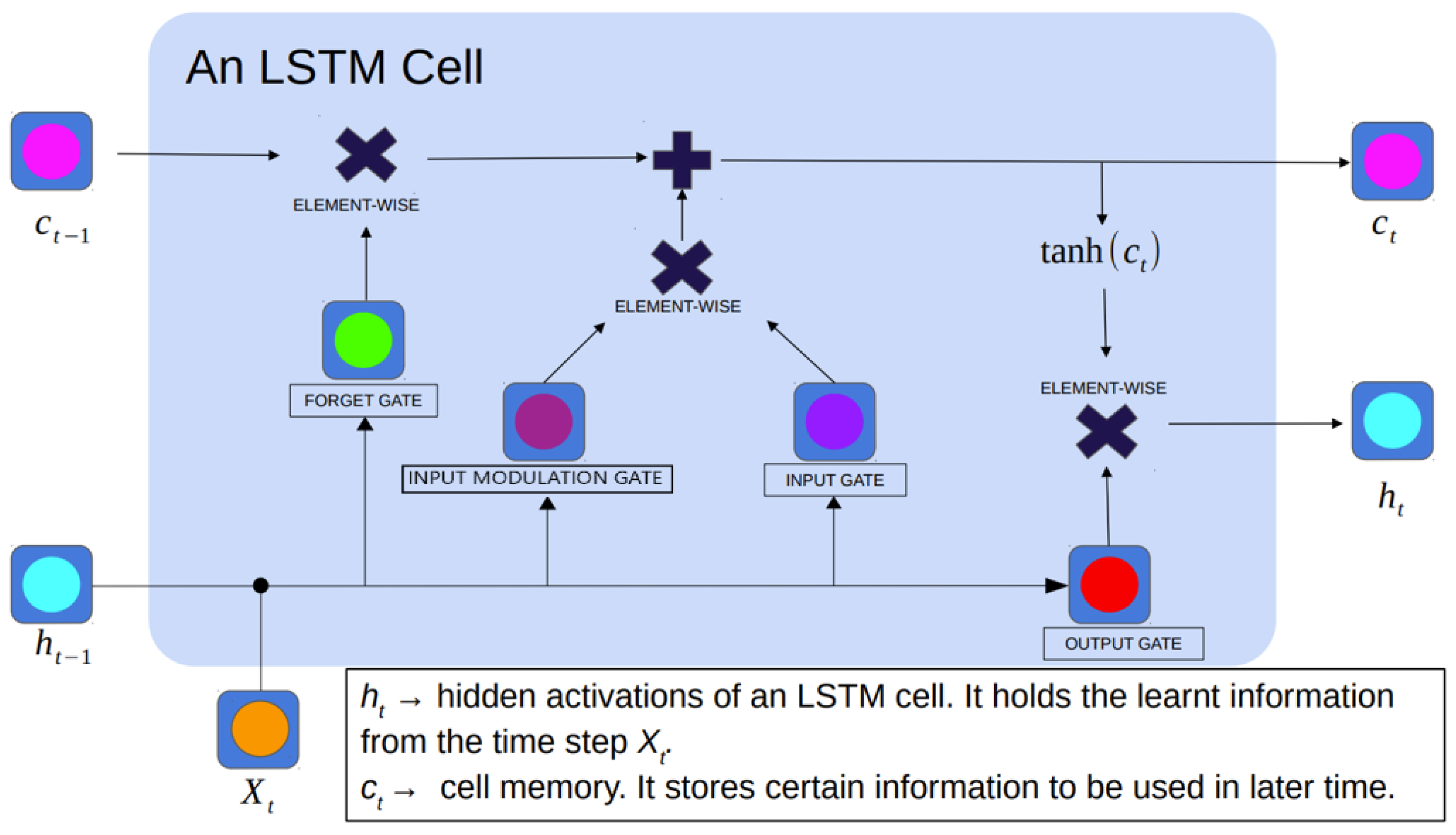
Depending on the type of inputs, different algorithms in neural networks could be used. Long Short-Term Memory Neural Networks [LSTM] [40,41] are known to produce desirable results while dealing with time-series data. LSTM is a Recurrent Neural Network that analyzes time series data and receives inputs as well as its own outputs from the previous time step to make predictions at the current time step. Although the basic concept of mapping the inputs and outputs remains the same, the training algorithm in LSTM differs from a regular multi-layer ANN model. The structure of an LSTM cell is demonstrated in Figure 1.
The current input vector and the previous short-term state are fed to four different, fully connected layers, which serve different purposes [42]. The main layer is the one that outputs , which has the usual role of analyzing the current inputs and the previous state . The other three layers are gate controllers, in which the logistic activation function is used. The forget gate controls which parts of the long-term state should be erased. The input gate controls which parts of should be added to the long-term state. Finally, the output gate controls which parts of the long-term state should be read and output at this time step to . Equations (1)–(6) show the operations through which every time step of the data goes through to produce an output in an LSTM cell.
where , , , are the weight matrices of each of the four layers for their connection to the input vector . , , , are the weight matrices of each of the four layers for their connection to the previous short-term state . , , , are the bias terms for each of the four layers. The weights and biases are determined through model training and are responsible for learning the mapping function between inputs and outputs. The outputs from the LSTM cell are usually not in the desirable shape; thus, a batch normalization layer or dense layer is required to produce the desired outputs.
2.2. Architecture
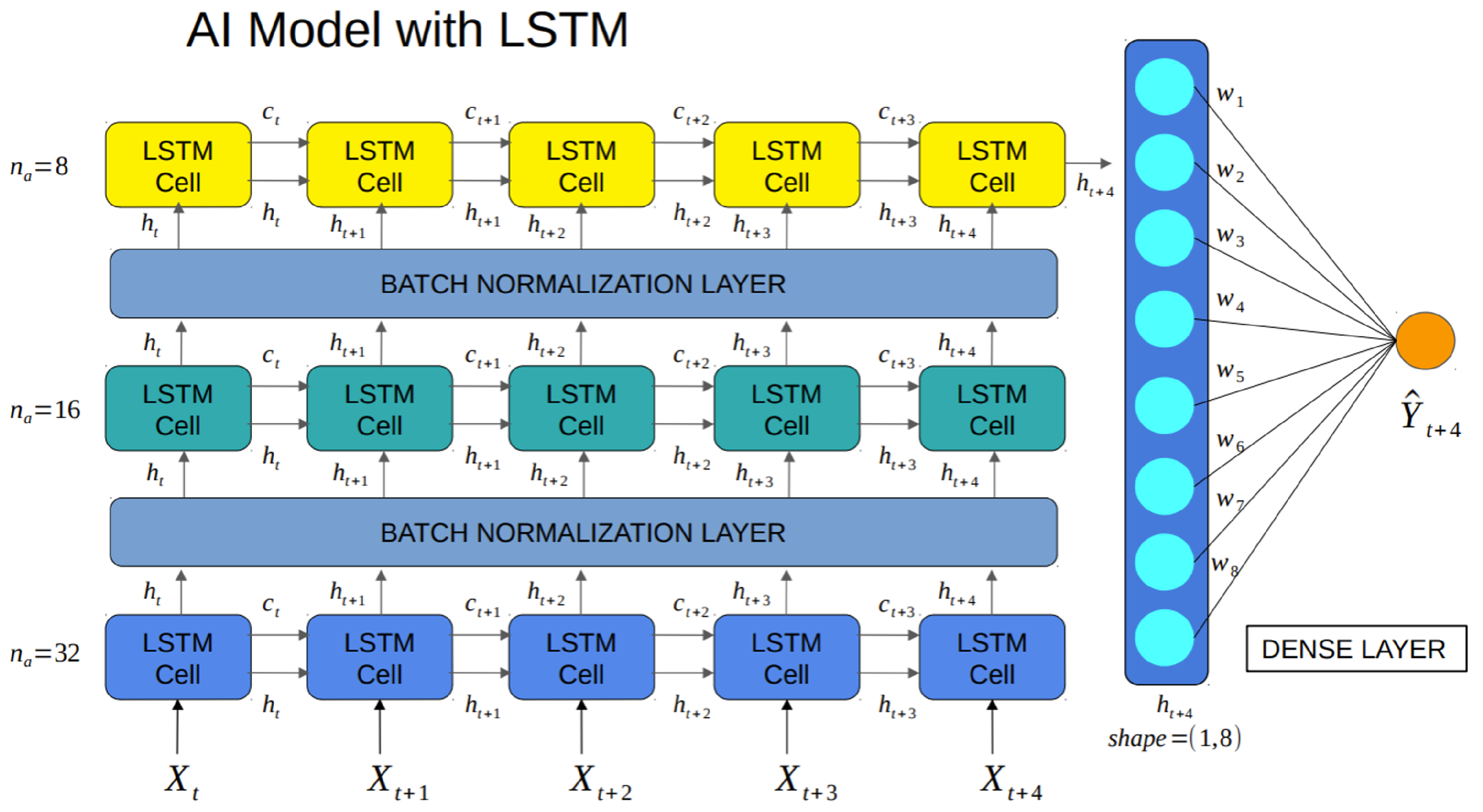
The architecture of the LSTM model for the Great Lakes is demonstrated in Figure 2, which consists of three LSTM layers, two batch normalization layers, and a dense layer. The model takes five days of historical feature data and predicts the target on the fifth day. The hyperparameters of the model are determined through trial and error to reach the best model performance. The test values and the optimal values of the hyperparameters are given in Table 1. The first LSTM layer has 32 neurons, which takes the five days of historical feature data as inputs. Its outputs are fed into a batch normalization layer to normalize the inputs for the second LSTM layer, which includes 16 neurons. The third LSTM layer has eight neurons and takes inputs from the second batch normalization layer. Its outputs are fed to a dense layer, which finally predicts the results. During model training, additional dropout layers with a dropout rate of 0.2 are added to avoid overfitting.
2.3. Data Processing
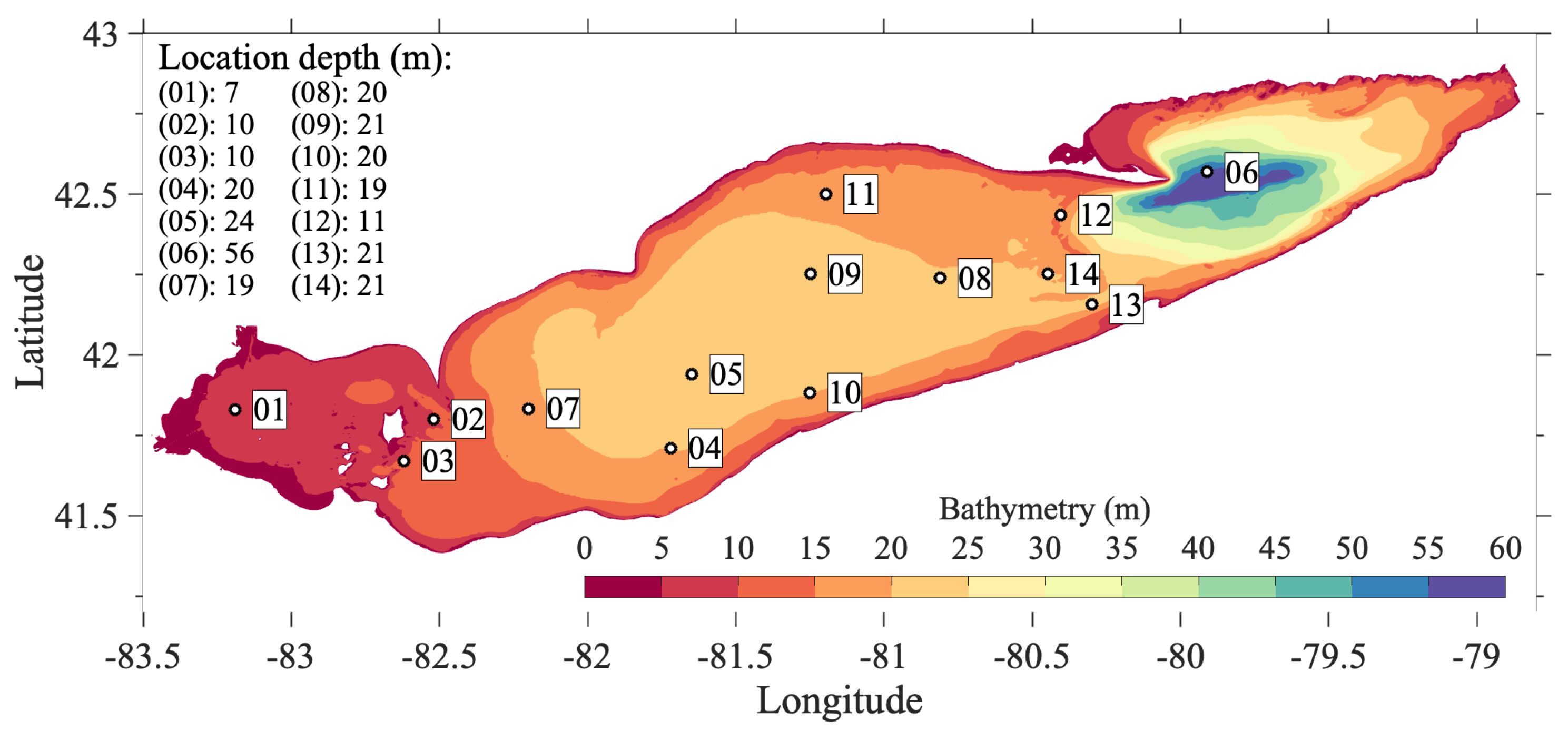
The LSTM input features consist of seven meteorological variables that are critical to the LST variation, including downward shortwave, downward longwave, latent heat, sensible heat, surface air temperature, zonal wind speed, meridional wind speed, with water depth as an optional eighth input feature. The target variable for the LSTM prediction is the LST. In this study, we evaluated the feasibility of using observations from the proposed hypothetical monitoring network(s) in each lake to train the LSTMs. For example, we test a hypothetical monitoring network in Lake Erie consisting of 14 observing sites that were designed in the International Field Years of Lake Erie (IFYLE) program in 2005 (Figure 3) to train the LSTM model for Lake Erie. It is referred to as a “hypothetical” monitoring network because there are no long-term (decade-long) observations in these proposed monitoring locations, as it was a seasonal monitoring effort in the summer of 2005. Therefore, we extracted the required variables at the proposed 14 sites from the reanalysis datasets for the LSTM training. After that, we evaluated the LSTM performance in predicting the LST over the entire lake with gridded over-lake meteorological inputs. The LSTM performance, in turn, can be used to evaluate the effectiveness of the proposed monitoring network in assisting the ML-based forecast. Such a method has been widely used in the Observing System Simulation Experiments (OSSEs) [43,44,45,46]. The same procedure and analysis are conducted for each lake.
The 7 meteorological features at the 14 hypothetical monitoring sites were extracted from the Climate Forecast System Reanalysis (CFSR) dataset for 1995–2010 and from the CFSR’s upgraded extension (i.e., Climate Forecast System Version 2 (CFV2)) available from 2011 to present at the National Center for Environmental Prediction (NCEP) [47]. For simplicity, we refer to both datasets as CFSR. CFSR is global reanalysis data with the assimilation of satellite radiances and all available conventional and satellite observations, and has been used to drive hydrodynamic models for the Great Lakes in various studies [13,17,48,49].
The target variable (daily LSTs) at the 14 hypothetical monitoring sites was extracted from the Great Lakes Surface Environmental Analysis (GLSEA; https://coastwatch.glerl.noaa.gov/glsea/glsea.html, accessed on 26 May 2022) developed by the NOAA Great Lakes Environmental Research Lab (GLERL). The data are derived from the Advanced Very High-Resolution Radiometer (AVHRR) satellite imagery and updated daily with information from the cloud-free portions of the previous day’s satellite imagery. GLSEA products applied a smoothing algorithm to generate a continuous evolution of the LST as described in Schwab et al. [50]. The GLSEA-LST is currently the best available resource to examine the spatial and temporal variability of LST for the entire Great Lakes [2,3,51].
The training dataset includes 17 years (1995–2011) of 6205 daily data (29 February in leap years were ignored) at 14 locations. At each location, the dataset was grouped into two matrices, including an input matrix with the shape of (6205 days, 7 features) and a labeled output matrix of (6205 days, 1 target). In the designed LSTM, we used 5 days of historical feature data to predict the LST. Hence, the inputs were further temporalized into 6205 daily instances, each of which includes the historical 5-day feature data. For instance, to predict the LST on the 5th day, the selected features on the 1st, 2nd, 3rd, 4th, and 5th days were used as inputs. Thus, the resultant input matrix had a shape of (6205, 5, 7) for each point. Finally, the temporalized data for all 14 sites were stacked to create the input dataset for training, which had a shape of (86,870 (i.e., 6205 × 14), 5, 7). Correspondingly, the output dataset for training had a shape of (86,870 (i.e., 6205 × 14), 1).
An important transformation in the data processing for machine learning models is feature scaling. This is critical when input attributes have very different scales, as in this study. A standardization transformation was performed to make all the input features and the target on the same scale. The Standard Scaler function in the scikit-learn package was employed for this task. The mean and variance of the training dataset were stored and used to standardize the testing dataset.
2.4. LSTM Training and Validation
For each of the Great Lakes, an LSTM model was developed following the same procedure. The LSTM was implemented using the Keras API in the TensorFlow open-source platform. The training and validation of the LSTM were performed in Google Colab using GPU acceleration. The LSTM for the input datasets with and without the water depth feature were trained separately. The training dataset (1995–2011), after standardization and temporalization, was randomly shuffled into a training dataset and a validation dataset with a ratio of 95:5. The hyperparameters of the models, such as the number of activations, number of LSTM layers, and number of epochs, were determined through trial and error to produce the best model performance. The optimal values of these hyperparameters are given in Table 1. Two optimizers (i.e., Adam and Stochastic Gradient Descent (SGD)) were tested. The Adam optimizer converged faster and produced slightly better model performance. Therefore, the Adam optimizer and the mean-square-error (MSE) loss function were employed to train all the LSTM models. To avoid model overfitting or underfitting, the number of LSTM layers and the number of nodes in each layer must be properly chosen. By using a grid search technique, it was determined that three LSTM layers with activation units of (32, 16, 8) produced better performance. In addition, a dropout method was applied to avoid model overfitting. Two dropout layers with a dropout rate of 0.2 were added after the first and second LSTM layers. Other parameters, such as learning rate, epochs, batch size, and validation split, were determined by optimizing the model performance.
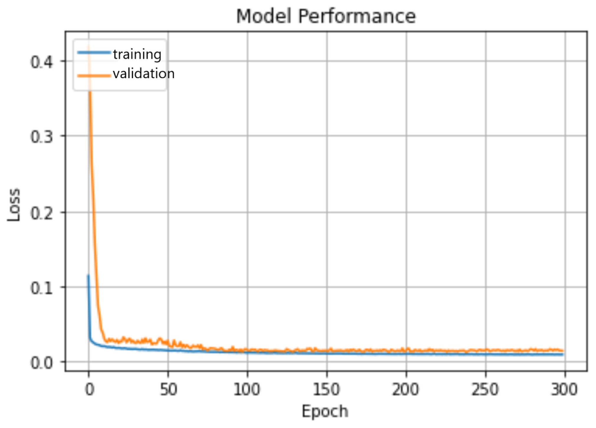
LSTM validation was carried out by comparing the LSTM performances on the training and validation datasets to determine whether the model is overfitting, underfitting, or well trained. If a model has good performance on the training data but poor generalization to the validation data, it is considered overfitting. If a model has poor performance on both the training and validation data, it is deemed to be underfitting. On the other hand, a well-trained model should perform well on both the training and validation datasets. During model validation, the model parameters determined from training, including all the hyperparameters, weights, and bias terms, remain unchanged. The validation dataset that was not used for training was fed into the model to produce the predictions. The model performance was evaluated by computing the MSE error between the model predictions and the labeled data in the validation dataset. Figure 4 shows the model performances on the training and validation datasets in Lake Erie. The training and validation errors reached a sufficiently low level with increased epochs. The loss functions decreased rapidly with increasing epochs (which defines the number of times that the learning algorithm will work through the entire training dataset) to a low level as the weights and bias terms in the model were optimized through model training. The model performance on both the training and validation data reached its optimized state with greater than 100 epochs, indicating that the model was well trained and did not suffer from overfitting or underfitting. Similar performances were observed in the training and validation for other lakes.
2.5. LSTM Prediction
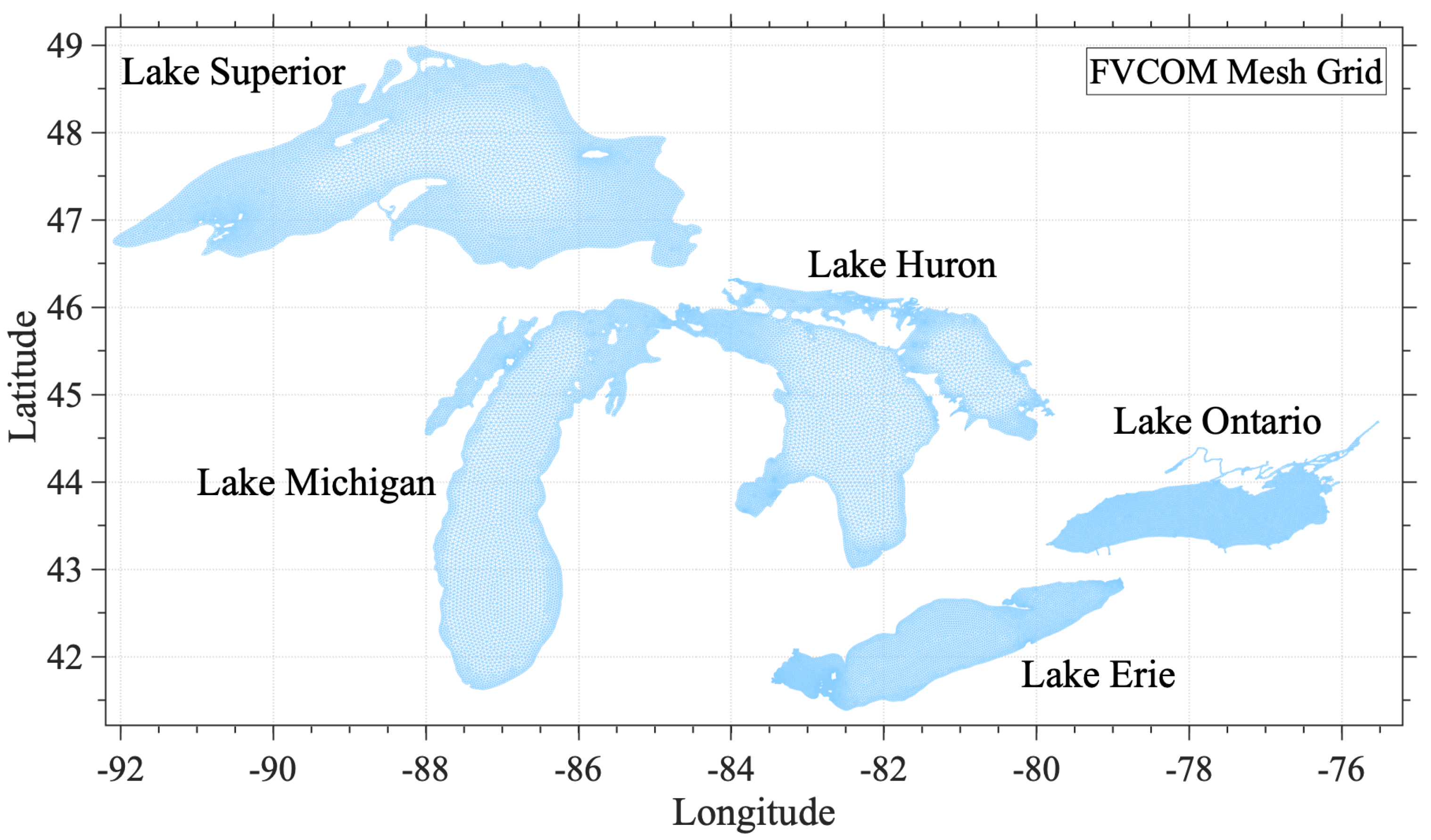
The above validation confirms that the trained LSTM can predict the LST at the 14 selected hypothetical monitoring locations. However, the goal of this study is to evaluate if the trained LSTM is capable of predicting the LST spatiotemporal patterns over the entire lake. We generated mesh grids (Figure 5) that cover the entirety of each lake to employ the trained LSTM to predict the LST at each mesh grid based on its meteorological features extracted from the CFSR dataset. The same grid mesh is used for a hydrodynamic model described in the next section. Therefore, the LSTs predicted from the LSTM and the hydrodynamic model are consistent for direct comparison.
3. Hydrodynamic Modeling
In parallel to deep learning, we applied a physics-based hydrodynamic model to simulate the surface temperatures in the Great Lakes to identify the strengths and weaknesses of ML and mechanistic modeling. The hydrodynamic model used in this study is based on the Finite Volume Community Ocean Model (FVCOM) [52]. FVCOM is a free-surface, primitive equation hydrodynamic model that solves the momentum, continuity, temperature, salinity, and density equations and is closed physically and mathematically using turbulence closure submodels. FVCOM is solved numerically using the finite-volume method in the integral form of the primitive equations over an unstructured triangular grid mesh and vertical sigma layers. The model grid resolution varies from 1–2 km near the coast to 2–4 km offshore (Figure 5), with a total of 35,000 model grids and 40 vertical sigma layers. The Mellor–Yamada level-2.5 (MY25) turbulence closure model [53] was used for simulating vertical mixing processes, and the horizontal diffusivity was calculated based on horizontal velocity shear and grid resolution using the Smagorinsky numerical formulation [54]. The FVCOM model was run in the two-way coupled atmosphere–lake system [3] and driven by hourly surface meteorological forcing, including incoming shortwave and longwave radiations, air temperature, atmospheric pressure, wind fields, total cloud cover, and relative humidity.
4. Results
4.1. LST Spatiotemporal Pattern from the LSTM Prediction
As presented in Section 2, we established the LSTM to predict the LST for each of the Great Lakes, including Lake Superior, Lake Michigan, Lake Huron, Lake Ontario, and Lake Erie. As Lake Erie has several concerning environmental issues associated with lake temperature (e.g., harmful algal blooms, large-scale hypoxic conditions), we use Lake Erie as an example to present detailed model results and analyses. The LSTM performances in the other four lakes are consistent and presented in Section 4.5.
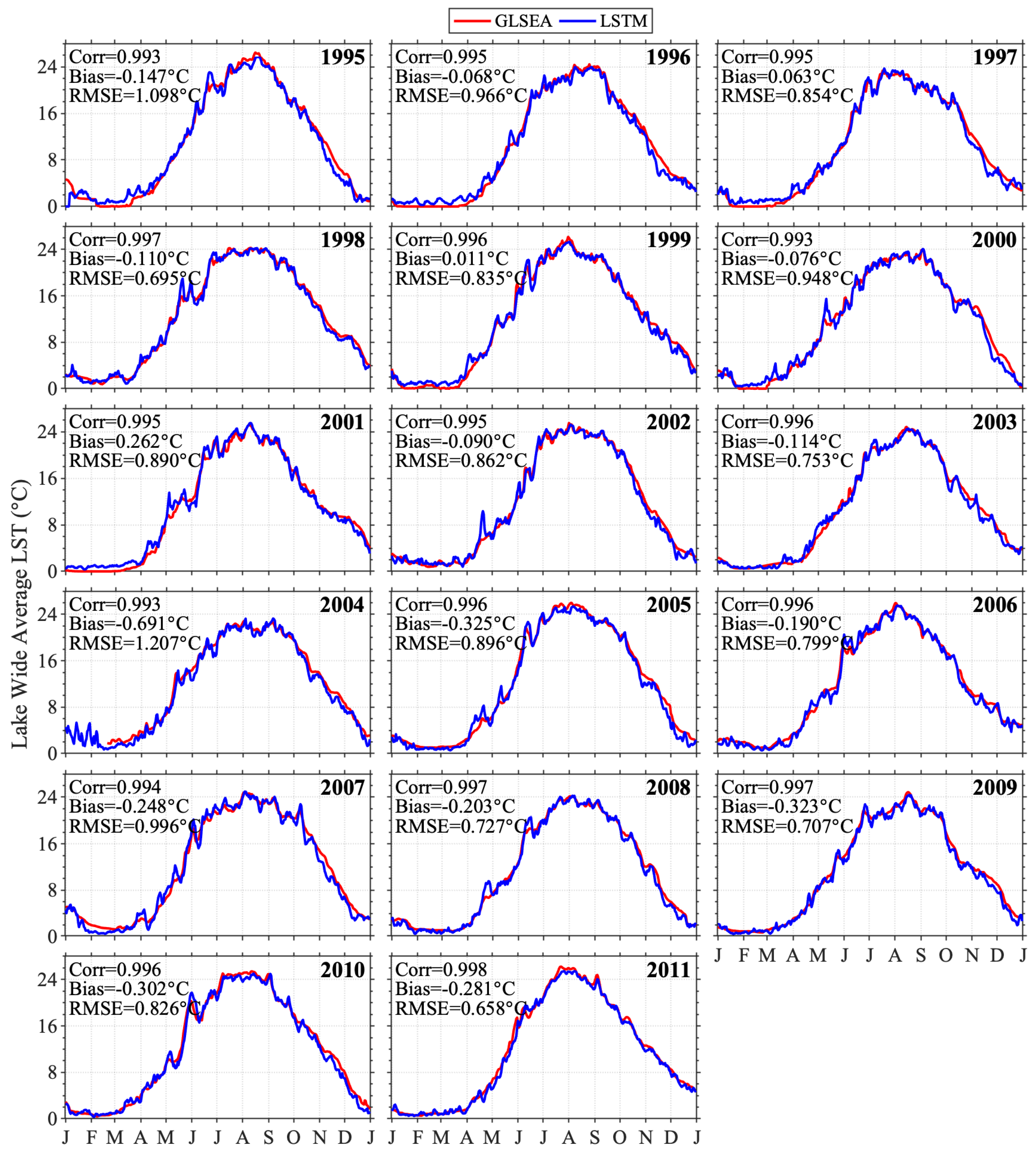
We highlight the LSTM predictions of the two most important LST characteristics of the Great Lakes ecosystem: the temporal evolution of lake-wide average LST and the seasonal spatial patterns of LST. Figure 6 presents the daily lake-wide average surface temperature for 1995–2011. The LSTM performed very well in predicting the temporal variations of the surface temperature in all years in comparison to the GLSEA data. Both the seasonal and interannual variabilities are well captured by the LSTM. The model accurately reproduced seasonal variability for the warmer years (e.g., 2005, 2010) and the cold years (e.g., 2000, 2004). The correlations between LSTM predictions and GLSEA data are very high at the daily scale (>0.99), low in annual mean bias (±0.3 °C), and the root-mean-square-errors (RMSE) (0.5–1.0 °C) across all years.
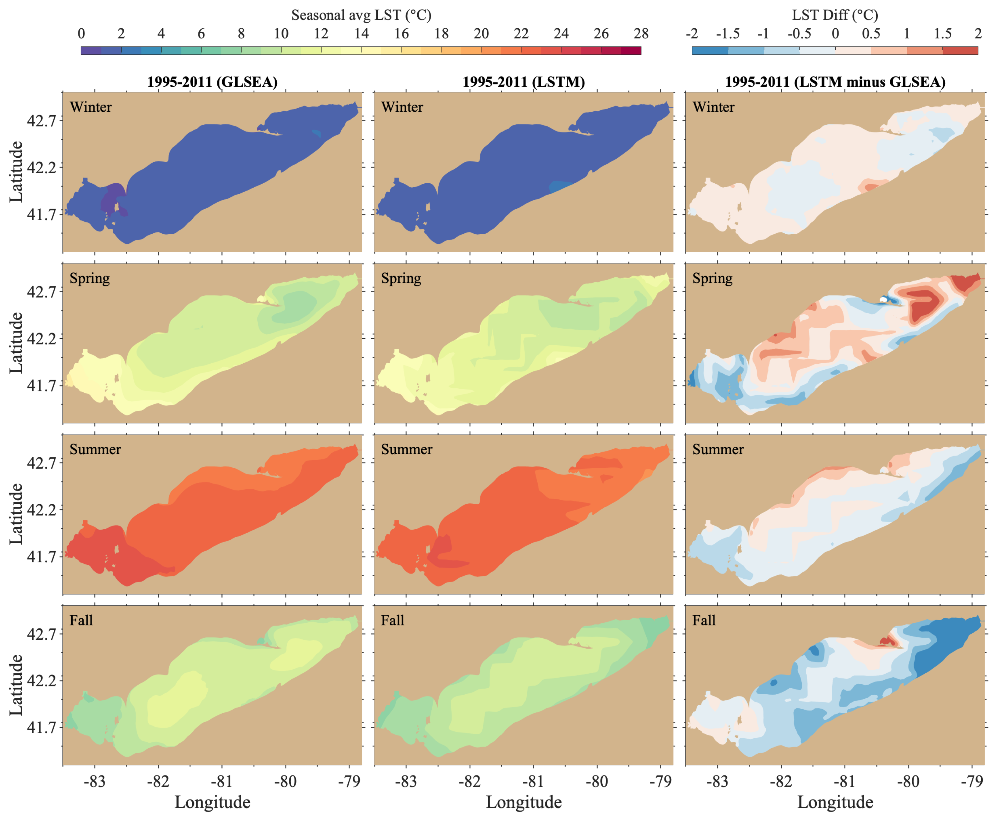
Figure 7 presents the spatial climatology of LSTs averaged over the 17-year prediction by the LSTM in comparison to the GLSEA reanalysis data. The LST is generally homogeneous in winter. In spring, the lake temperature warms progressively from the shallow western basin and southern coastal water to the deep water in the central and eastern basins when the stratification is developing with cross-slope LST gradients. The warmest surface water exists in the whole lake in summer, with relatively warmer waters in the shallow western basin and cooler water along the north coast. In fall, the LST decreases first in the western basin due to its shallowness, while the waters in the deep central and eastern basins are still relatively warm. The LSTM predicted the spatial patterns of the water temperature reasonably well, particularly during summer and winter, with biases less than 0.5 °C in most regions. However, relatively large warm (1–2 °C) biases appeared in the central and northern basins in spring and cold biases (1–2 °C) in these regions in fall.
4.2. LST Spatiotemporal Pattern from the FVCOM Prediction
The above results confirmed that the LSTM can be an efficient and effective tool for LST prediction, yet, physics-based hydrodynamic modeling is still considered the most fundamental approach. The hydrodynamic model resolves the physical processes described by primitive equations that satisfy the conservation of mass, momentum, and energy. Therefore, the hydrodynamic model simulates the time evolution of entire 3-D hydrodynamic processes (not only surface temperature), including water currents, surface elevation, temperature, eddy viscosity, and diffusivity. More importantly, it provides us with a mechanistic understanding of the system.
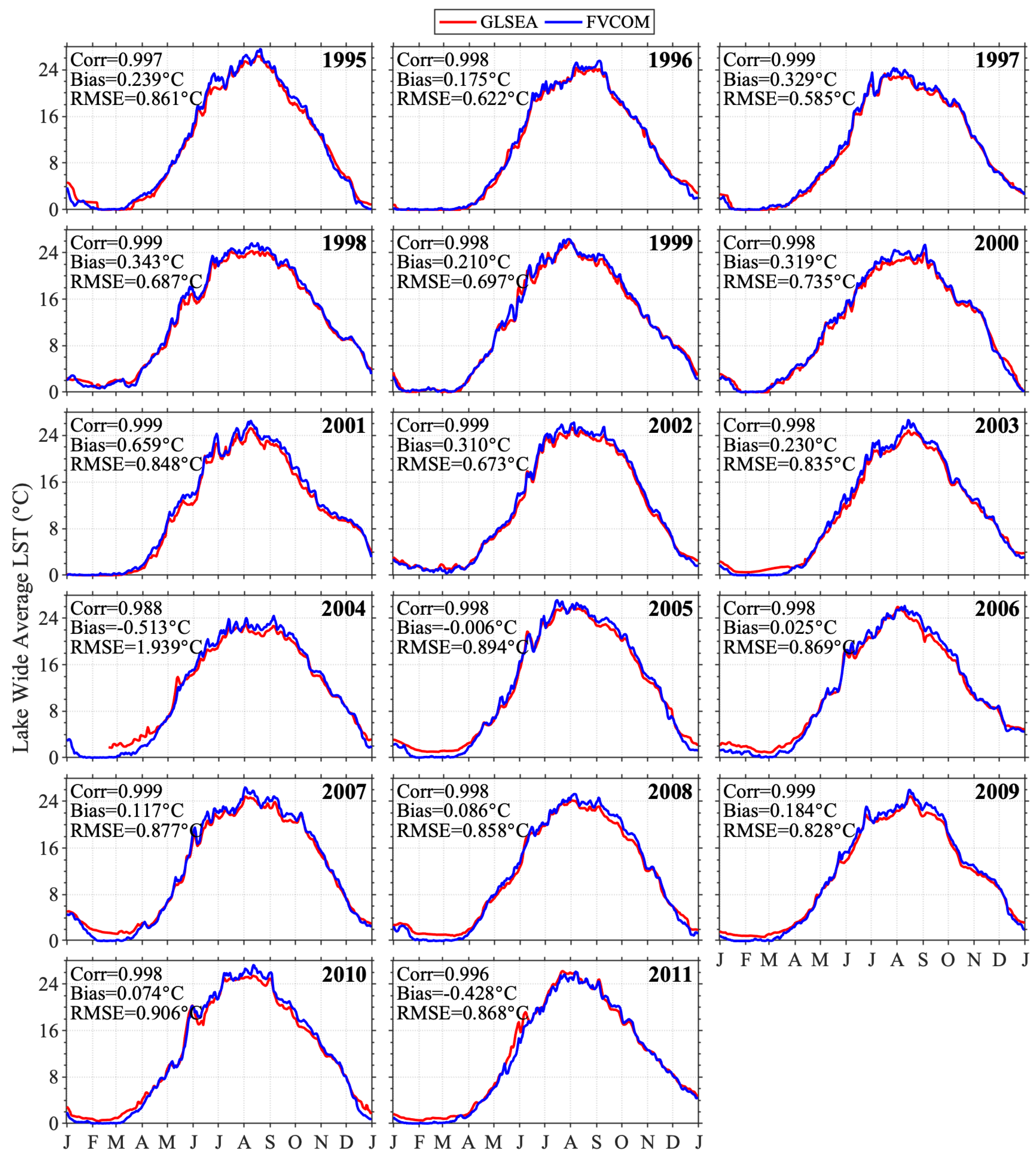
The results from the hydrodynamic model FVCOM are presented in Figure 8. Overall, the FVCOM also simulated the seasonal and interannual variability of the LST well. However, the model over-predicted the summer surface temperature in most of the years, with some most noticeable summer warm biases in 1998, 2000, 2004, 2006, and 2009. This is also shown in the model simulated seasonal spatial pattern and error distribution of the LST (Figure 9). The FVCOM simulation showed a close agreement with GLSEA data in the winter, spring, and fall seasons in terms of detailed spatial patterns and temperature gradients in the lake. However, in the summer, a noticeable warm bias (1–2 °C) exists in the region below the latitude of 42.2 degrees as well as in the northern end of the lake. The model predicted a stronger meridional temperature gradient than was observed in the GLSEA. Note that the exception for the comparison is the surface temperature difference near the northern coast. The narrow strip of cold water is caused by local upwelling, which is realistically resolved by the hydrodynamic model and is often missed in the GLSEA dataset due to its lower accuracy near the coast.
4.3. Integration of Hydrodynamic Model and LSTM
The above analyses show that both LSTM and FVCOM can predict the LST reasonably well, yet with different bias characteristics. Therefore, we explore the approach to integrating both predictions to optimize the estimation of lake status. In this study, we test a variational method to incorporate the results from the LSTM and FVCOM to further improve prediction accuracy.
Denote the LST as a state vector . and are results from FVCOM and LSTM with respective error covariance matrices and . The Best Linear Unbiased Estimator (BLUE) theory states that the best linear estimate () is the solution to the following variational optimization problem:
where is called the cost function of the analysis (or misfit, or penalty function) for the hydrodynamic model penalty term and LSTM penalty term .
Applying Equations (10) and (11) to each model grid point for localization, the best linear estimate () at a given grid point i is:
where and are the root mean squared error (RMSE) of the FVCOM and LSTM predictions relative to the GLSEA at grid point i. The and were calculated for each season, respectively, based on the results for 1995–2011. For the upwelling region along the northern coast, we assigned normalized empirical weights of 0.8 and 0.2 to the FVCOM and LSTM predictions since only the hydrodynamic model simulation resolved the local upwellings.
The improvement of LST estimation through the LSTM-FVCOM integration is significant and evident in Figure 10 and Figure 11. Temporally, integrating the LSTM and FVCOM model results improved the LST predictions during all seasons. As summarized in the seasonal climatology (Figure 10), the warm biases (RMSE of 0.72 °C) in lake-wide average surface temperature during summer in the FVCOM results are largely removed, and so are the cold bias with (RMSE of 0.65 °C) during the winter. Similarly, the cold bias (RMSE of 0.8 °C) in the LSTM prediction during the fall is also effectively corrected. The integration produced a more accurate estimate of LST than the individual prediction from either LSTM or FVCOM.
Spatially, the LSTM and FVCOM integration efficiently reduced spatial errors in all seasons (Figure 11). The biases are minimized to ( °C) for nearly the entire lake, except for a small area at the northern end of the lake in spring. The integration significantly reduced the relatively large errors in the central and northern basins from the LSTM prediction during spring and fall (Figure 7 vs. Figure 11) as well as the summer warm bias in the majority of the lake in the hydrodynamic modeling (Figure 9 vs. Figure 11). More importantly, the spatial temperature gradients and variability across the slope from shallow water to deep water and between the basins are well captured, reinforcing the enhanced prediction accuracy through the integration. The integrated results also retain upwelling regions as expected.
4.4. Prediction beyond the Training Period
The results in Section 4.1 show that the LSTM trained with limited data from the hypothetical monitoring network has the ability to predict the spatial and temporal patterns in the entire lake over the training period. This section examines whether the LSTM can be used to make predictions beyond the training period. We extended the LSTM prediction for a 5-year period (2012–2016) beyond the training period (1995–2011) with exact parameters, including all the hyperparameters, weights, and bias terms unchanged. The satisfactory performance of the LSTM is well retained for 2012–2016. The LSTM accurately captured the seasonal variation of LST as well as its interannual variability, indicated by the envelopes (Figure 12). The results during the 5-year period appeared to be even slightly better than in the training period due to the upgraded, higher-resolution CFSR meteorological dataset after 2011 (i.e., CFV2, see Section 2.3). Improvement in hydrodynamic simulations due to the upgrade of CFSR since 2011 has also been documented in other studies [49].
4.5. Evaluation of the LSTM Performance for Other Lakes
The LSTMs for each lake were trained using data from 14 points following the same approach we used for Lake Superior, as described in Section 2.3 and Section 2.4. The results are consistent with what we presented for Lake Erie, as summarized in Figure 13. The predictions for all lakes retain high correlations (>0.99) with the GLSEA reanalysis, low mean biases (0.02–0.77 °C), and low RMSE values (0.3–0.9 °C). The consistent LSTM performance across the five lakes suggests that the findings from Lake Erie’s analysis are applicable to the other four lakes, such as the integration of deep learning and hydrodynamic modeling. It should be noted that the selection of the 14 hypothetical monitoring sites in the four lakes was fairly arbitrary (there was no trial-and-error or iterative tuning for selecting sites). The site selection was completed in a one-time attempt with a general principle that the sites chosen should have good coverage over the entire lake and represent both deep basins and coastal waters. The satisfactory results under such conditions reinforce the robustness of the LSTM performances. Lastly, we acknowledge that the selection of the monitoring sites may be further optimized to achieve better results to some extent, although this is beyond the scope of this study.
4.6. Effect of Water Depth
Water depth (bathymetry) is one of the most critical inputs in a physics-based hydrodynamic model. However, it is unclear whether it is an essential feature for LSTM training. The water depth is spatially varying but remains constant temporally. To examine its impact on LSTM performance, we added water depth as the eighth feature and re-trained the LSTM. Neural networks, in general, can learn to disregard non-essential input features during training. The features affecting more on the target are weighted more than the less relevant features. By comparing the model skills with and without the water depth feature, we found that the water depth feature was deemed redundant in the LSTM in our case. The skill metrics such as correlation, mean bias, and RMSE remain similar in the two LSTMs trained with or without the water depth feature, and adding the water depth feature does not further improve the LSTM prediction. This is likely because water depth is temporally constant, and, therefore, its effects can be directly modeled by the bias terms in the LSTM.
5. Discussion
5.1. Understanding of Model Performance
While deep learning models are often considered as blackboxes, there is a growing need to understand the relationship between features and predictions. To that end, we employed an explainable artificial intelligence (XAI) technique named SHapley Additive exPlanations (SHAP) to uncover how the features impact the predictions [55]. SHAP can be used for explaining the prediction of an ML model by computing the contribution of each feature to the prediction. The SHAP analysis shows that the air temperature is the most influential feature of the LST prediction, with a significantly larger SHAP value than the other features (Figure 14a). Notice that the results suggest a strong correlation (which can be nonlinear) between the air temperature and LST, rather than indicating the causal relationship between the two, as physical conditions near the lake-atmosphere interface strongly influence both variables. The SHAP analysis also supports previous efforts that aimed to utilize the air temperature to reconstruct the lake temperature by developing simplified empirical functions [56,57]. These studies achieved certain success in reconstructing the lake-wide mean temperature but could not predict spatiotemporal patterns of LST as presented in this work using deep learning. In addition, the impact of the features on the LST is generally consistent with our mechanistic understanding of how LST would be affected by environmental factors, including the positive impact of air temperature, longwave radiation on the LST, and the negative impacts of latent and sensible heat fluxes, and wind speed (Figure 14b).
Knowing that the air temperature is the most influential feature, we hypothesize that the relatively large bias in LSTM prediction during the spring and fall is closely associated with spatial anomalies in both air temperature and LST. The most substantial heterogeneity of air temperature occurs during the spring and fall with a spatial variability of ±2 °C, while it is fairly homogeneous during the winter and summer with a spatial variability of less than 0.8 °C (Figure 15a). The strong correlation of spatial patterns between air temperature and LST anomalies reinforces the SHAP analysis (Figure 15b).
However, from the hydrodynamic modeling perspective, simulating the summer thermal structure is more challenging, partly due to the strong summer stratification. In the central basin, the hydrodynamic model often underestimates the mixed-layer depth and results in a warmer surface layer [8]. In addition, modeled temperature and circulation patterns are also sensitive to the anticyclonic wind vorticity, which can also lead to thinning of the hypolimnion in the central basin [12]. In the western basin, where the water depth is much shallower and often unstratified, the warm bias is most sensitive to surface heat flux with much less buffering effect due to its shallowness. To test the impact of atmospheric forcing uncertainty on the hydrodynamic modeling, we also conducted the simulation in which the FVCOM model is driven by in situ observation-interpolated forcing [13]. With this forcing, LST biases were reduced during the summer but caused more significant warm biases (not shown) during the fall due to the underestimated surface heat fluxes and wind speed.
5.2. Future Model Improvement
In the current study, the LST prediction at each grid cell is independent and determined by input features over the grid cell and the previous LST at the grid. This is because we aimed to evaluate the feasibility of using scattered observational data from the proposed hypothetical monitoring network(s) in each lake to train the LSTMs. The results confirm that the current LSTM framework worked well with comparable accuracy to the hydrodynamic modeling. However, if aiming to use data with a more completed spatial coverage in the entire lakes (e.g., satellite images and reanalysis data), we can alternate the ML framework to consider the spatial changes in the LST and the atmospheric forcing from neighboring grids in the prediction. This can be achieved with a hybrid convolutional neural network (CNN) and LSTM approach, in which the model learns the spatial feature of atmospheric and lake variables by CNN and then utilizes LSTM to examine the temporal relations in lake thermal progression [58]. In addition, a possible approach is to learn the dynamics in the frequency domain using Fourier neural operator (FNO), which uses a Fourier layer that implements a Fourier transform, a linear transform, and an inverse Fourier transform for a convolution-like operation to extract mesh-independent spatiotemporal features [59,60,61].
In this study, we demonstrated a postprocessing framework to statistically integrate the LSTM and FVCOM results. We note that there are various ways in which deep learning approaches can help improve hydrodynamic modeling. For instance, deep learning has been used to approximate subscale processes to improve climate and ocean modeling [30,35]. Wang et al. [62] also applied a deep learning approach to reconstruct Reynolds stresses in RANS simulations of a turbulent flow. In these studies, deep learning approaches were used to predict the unclosed terms in a hydrodynamic model to improve the prediction accuracy and efficiency of the model. Meanwhile, deep learning can assist hydrodynamic modeling by optimizing ensemble averages of physics-based model predictions [31,32] and can be embedded in the hydrodynamic model to parameterize the air–sea feedback [34].
On the other hand, ML models can also be improved by injecting the physical constraints into the design of deep learning models to force the outputs of deep learning to respect physical laws related to mechanistic modeling [29,63]. For example, one can apply the energy balance rule in the loss function of deep learning models when predicting lake temperature. Moreover, simulated data generated from a physical model can be used to pre-train the deep learning model to allow deep learning to converge faster with a smaller number of ground truth samples [64]. Furthermore, deep learning models can also be used to more efficiently calibrate the physical model [65]. However, those approaches are yet to be tested for hydrodynamic modeling and will be part of our future study.
6. Summary and Conclusions
In this paper, we applied LSTMs to predict the spatiotemporal variation of LST, an essential environmental variable and climate indicator in the Great Lakes. Furthermore, we demonstrated an integrated framework that incorporates LST predictions from physics-based hydrodynamic modeling and data-driven deep learning to further enhance prediction accuracy. Compared to the previous ML applications to the Great Lakes prediction, our work advances the deep learning application in three aspects:
- Previous ML studies of the Great Lakes hydrodynamic forecast focused on wave predictions, which are controlled primarily by wind features. These studies either developed the emulator of the physics-based wave model in a single lake [36] or developed a wind-wave nonlinear relationship at a few specific sites [37]. Using seven meteorological features, this study is the first one to apply deep learning to predict the spatiotemporal patterns of the LSTs across the five Great Lakes.
- Our approach is highly efficient in developing systematic predictions across the Great Lakes. In the previous study [36], the training of the surrogate model required a large amount of training data generated from the physics-based wave model. This approach has two drawbacks (1) developing a physics-based model for all the five lakes becomes a prerequisite, and (2) the accuracy of the physics-based model constrains the deep learning performance. This study demonstrated the feasibility of training LSTMs with limited observations to make reliable predictions for the entire lake. The predictions from the LSTM models have consistent and robust performance across the lakes and are able to capture the temporal and spatial variabilities of LSTs for the entirety of the five Great Lakes. This is important as designing the observation network for data collection is primarily limited by the costs of deployment and maintenance.
- We further examined the features through an explainable AI technique (i.e., SHAP) to better understand their contributions to the model prediction. The SHAP analysis revealed air temperature is the most influential feature for predicting the LST in the trained LSTMs. The prediction bias is closely associated with substantial spatial heterogeneity of air temperature, particularly during spring and fall.
- Lastly, we demonstrated the integration of data-driven deep learning and mechanistic hydrodynamic modeling in the Great Lakes LST prediction. Our results showed that using the variational method to integrate the FVCOM and LSTM results can further enhance prediction accuracy. While the hydrodynamic model provides us with the mechanistic understanding and description of the Great Lakes system, a well-trained deep learning model could serve as an auxiliary tool to the hydrodynamic model simulation. Therefore, this work offers a new viable avenue for developing the next-generation Great Lakes forecast system.
Author Contributions
Conceptualization, P.X.; methodology, A.W., Y.W., C.H., P.X., G.M. and T.L.; software, A.W. and Y.W.; validation, C.H. and A.W.; formal analysis, P.X., C.H. and G.M.; resources, P.X. and Y.Y.; writing—original draft preparation, P.X., G.M. and A.W.; writing—review and editing, P.X., G.M., A.W. and T.L.; visualization, C.H.; supervision, P.X.; project administration, P.X.; funding acquisition, P.X. All authors have read and agreed to the published version of the manuscript.
Funding
This research was funded by the Michigan Tech Hydrodynamic Modeling Research Initiative. Funding was also provided by the National Oceanic and Atmospheric Administration (NOAA) Office of Oceanic and Atmospheric Research (OAR), through the University of Michigan Cooperative Institute for Great Lakes Research (CIGLR) cooperative agreement with NOAA (NA17OAR4320152). Hydrodynamic modeling was also supported, in part, by COMPASS-GLM, a multi-institutional project supported by the U.S. Department of Energy, Office of Science, Office of Biological and Environmental Research, Earth and Environmental Systems Modeling program.
Acknowledgments
This is contribution NO. 93 of the Great Lakes Research Center at Michigan Technological University. The Michigan Tech high-performance computing cluster, Superior, was used in obtaining the modeling results presented in this publication.
Conflicts of Interest
The authors declare no conflict of interest.
Abbreviations
The following abbreviations are used in this manuscript:
| LST | Lake Surface Temperature |
| ML | Machine Learning |
| ANN | Artificial Neural Network |
| LSTM | Long short-term memory |
| MLP | Multi-layer Perceptron |
| FVCOM | Finite Volume Community Ocean Model |
References
- U.S.EPA. State of the Great Lakes 2011; Technical Report, EPA 950-R-13-002; EPA: Washington, DC, USA, 2014. [Google Scholar]
- Shi, Q.; Xue, P. Impact of lake surface temperature variations on lake effect snow over the Great Lakes region. J. Geophys. Res. Atmos. 2019, 124, 12553–12567. [Google Scholar] [CrossRef]
- Xue, P.; Pal, J.S.; Ye, X.; Lenters, J.D.; Huang, C.; Chu, P.Y. Improving the simulation of large lakes in regional climate modeling: Two-way lake–atmosphere coupling with a 3D hydrodynamic model of the Great Lakes. J. Clim. 2017, 30, 1605–1627. [Google Scholar] [CrossRef]
- Notaro, M.; Zhong, Y.; Xue, P.; Peters-Lidard, C.; Cruz, C.; Kemp, E.; Kristovich, D.; Kulie, M.; Wang, J.; Huang, C.; et al. Cold Season Performance of the NU-WRF Regional Climate Model in the Great Lakes Region. J. Hydrometeorol. 2021, 22, 2423–2454. [Google Scholar] [CrossRef]
- Wang, J.; Xue, P.; Pringle, W.; Yang, Z.; Qian, Y. Impacts of Lake Surface Temperature on the Summer Climate Over the Great Lakes Region. J. Geophys.-Res.-Atmos. 2022; in press. [Google Scholar] [CrossRef]
- Austin, J.A.; Colman, S.M. Lake Superior summer water temperatures are increasing more rapidly than regional air temperatures: A positive ice-albedo feedback. Geophys. Res. Lett. 2007, 34. [Google Scholar] [CrossRef] [Green Version]
- Huang, C.; Kuczynski, A.; Auer, M.T.; O’Donnell, D.M.; Xue, P. Management transition to the Great Lakes nearshore: Insights from hydrodynamic modeling. J. Mar. Sci. Eng. 2019, 7, 129. [Google Scholar] [CrossRef] [Green Version]
- Ye, X.; Chu, P.Y.; Anderson, E.J.; Huang, C.; Lang, G.A.; Xue, P. Improved thermal structure simulation and optimized sampling strategy for Lake Erie using a data assimilative model. J. Great Lakes Res. 2020, 46, 144–158. [Google Scholar] [CrossRef]
- Wuebbles, D.; Cardinale, B.; Cherkauer, K.; Davidson-Arnott, R.; Hellmann, J.; Infante, D.; Ballinger, A. An Assessment of the Impacts of Climate Change on the Great Lakes; Environmental Law & Policy Center: Chicago, IL, USA, 2019. [Google Scholar]
- Xue, P.; Ye, X.; Pal, J.S.; Chu, P.Y.; Kayastha, M.B.; Huang, C. Climate Projections over the Great Lakes Region: Using Two-way Coupling of a Regional Climate Model with a 3-D Lake Model. Geosci. Model Dev. Discuss. 2022; in press. [Google Scholar]
- Notaro, M.; Holman, K.; Zarrin, A.; Fluck, E.; Vavrus, S.; Bennington, V. Influence of the Laurentian Great Lakes on regional climate. J. Clim. 2013, 26, 789–804. [Google Scholar] [CrossRef] [Green Version]
- Beletsky, D.; Hawley, N.; Rao, Y.R. Modeling summer circulation and thermal structure of Lake Erie. J. Geophys. Res. Ocean. 2013, 118, 6238–6252. [Google Scholar] [CrossRef] [Green Version]
- Xue, P.; Schwab, D.J.; Hu, S. An investigation of the thermal response to meteorological forcing in a hydrodynamic model of Lake Superior. J. Geophys. Res. Ocean. 2015, 120, 5233–5253. [Google Scholar] [CrossRef]
- Fujisaki, A.; Wang, J.; Bai, X.; Leshkevich, G.; Lofgren, B. Model-simulated interannual variability of Lake Erie ice cover, circulation, and thermal structure in response to atmospheric forcing, 2003–2012. J. Geophys. Res. Ocean. 2013, 118, 4286–4304. [Google Scholar] [CrossRef]
- Liu, Q.; Anderson, E.J.; Zhang, Y.; Weinke, A.D.; Knapp, K.L.; Biddanda, B.A. Modeling reveals the role of coastal upwelling and hydrologic inputs on biologically distinct water exchanges in a Great Lakes estuary. Estuar. Coast. Shelf Sci. 2018, 209, 41–55. [Google Scholar] [CrossRef]
- Anderson, E.J.; Fujisaki-Manome, A.; Kessler, J.; Lang, G.A.; Chu, P.Y.; Kelley, J.G.; Chen, Y.; Wang, J. Ice forecasting in the next-generation Great Lakes operational forecast system (GLOFS). J. Mar. Sci. Eng. 2018, 6, 123. [Google Scholar] [CrossRef] [Green Version]
- Ye, X.; Anderson, E.J.; Chu, P.Y.; Huang, C.; Xue, P. Impact of water mixing and ice formation on the warming of Lake Superior: A model-guided mechanism study. Limnol. Oceanogr. 2019, 64, 558–574. [Google Scholar] [CrossRef]
- Cushman-Roisin, B.; Beckers, J.M. Introduction to Geophysical Fluid Dynamics: Physical and Numerical Aspects; Academic Press: Cambridge, MA, USA, 2011. [Google Scholar]
- Xue, P.; Malanotte-Rizzoli, P.; Wei, J.; Eltahir, E.A. Coupled ocean-atmosphere modeling over the Maritime Continent: A review. J. Geophys. Res. Ocean. 2020, 125, e2019JC014978. [Google Scholar] [CrossRef]
- Ibrahim, H.D.; Xue, P.; Eltahir, E.A. Multiple salinity equilibria and resilience of Persian/Arabian Gulf basin salinity to brine discharge. Front. Mar. Sci. 2020, 7, 573. [Google Scholar] [CrossRef]
- Fujisaki, A.; Wang, J.; Hu, H.; Schwab, D.J.; Hawley, N.; Rao, Y.R. A modeling study of ice–water processes for Lake Erie applying coupled ice-circulation models. J. Great Lakes Res. 2012, 38, 585–599. [Google Scholar] [CrossRef]
- Huang, C.; Anderson, E.; Liu, Y.; Ma, G.; Mann, G.; Xue, P. Evaluating essential processes and forecast requirements for meteotsunami-induced coastal flooding. Nat. Hazards 2021, 110, 1693–1718. [Google Scholar] [CrossRef]
- Sun, L.; Liang, X.Z.; Xia, M. Developing the Coupled CWRF-FVCOM Modeling System to Understand and Predict Atmosphere-Watershed Interactions Over the Great Lakes Region. J. Adv. Model. Earth Syst. 2020, 12, e2020MS002319. [Google Scholar] [CrossRef]
- Chapman, W.; Subramanian, A.; Delle Monache, L.; Xie, S.; Ralph, F. Improving atmospheric river forecasts with machine learning. Geophys. Res. Lett. 2019, 46, 10627–10635. [Google Scholar] [CrossRef]
- McGovern, A.; Elmore, K.L.; Gagne, D.J.; Haupt, S.E.; Karstens, C.D.; Lagerquist, R.; Smith, T.; Williams, J.K. Using artificial intelligence to improve real-time decision-making for high-impact weather. Bull. Am. Meteorol. Soc. 2017, 98, 2073–2090. [Google Scholar] [CrossRef]
- Scher, S. Toward data-driven weather and climate forecasting: Approximating a simple general circulation model with deep learning. Geophys. Res. Lett. 2018, 45, 12–616. [Google Scholar] [CrossRef] [Green Version]
- Liu, Y.; Racah, E.; Correa, J.; Khosrowshahi, A.; Lavers, D.; Kunkel, K.; Wehner, M.; Collins, W. Application of deep convolutional neural networks for detecting extreme weather in climate datasets. arXiv 2016, arXiv:1605.01156. [Google Scholar]
- Scher, S.; Messori, G. Predicting weather forecast uncertainty with machine learning. Q. J. R. Meteorol. Soc. 2018, 144, 2830–2841. [Google Scholar] [CrossRef]
- Zhao, W.L.; Gentine, P.; Reichstein, M.; Zhang, Y.; Zhou, S.; Wen, Y.; Lin, C.; Li, X.; Qiu, G.Y. Physics-constrained machine learning of evapotranspiration. Geophys. Res. Lett. 2019, 46, 14496–14507. [Google Scholar] [CrossRef]
- Brenowitz, N.D.; Bretherton, C.S. Prognostic validation of a neural network unified physics parameterization. Geophys. Res. Lett. 2018, 45, 6289–6298. [Google Scholar] [CrossRef]
- O’Donncha, F.; Zhang, Y.; Chen, B.; James, S.C. An integrated framework that combines machine learning and numerical models to improve wave-condition forecasts. J. Mar. Syst. 2018, 186, 29–36. [Google Scholar] [CrossRef] [Green Version]
- O’Donncha, F.; Zhang, Y.; Chen, B.; James, S.C. Ensemble model aggregation using a computationally lightweight machine-learning model to forecast ocean waves. J. Mar. Syst. 2019, 199, 103206. [Google Scholar] [CrossRef] [Green Version]
- Wei, J.; Jiang, G.Q.; Liu, X. Parameterization of typhoon-induced ocean cooling using temperature equation and machine learning algorithms: An example of typhoon Soulik (2013). Ocean Dyn. 2017, 67, 1179–1193. [Google Scholar] [CrossRef]
- Jiang, G.Q.; Xu, J.; Wei, J. A deep learning algorithm of neural network for the parameterization of typhoon-ocean feedback in typhoon forecast models. Geophys. Res. Lett. 2018, 45, 3706–3716. [Google Scholar] [CrossRef] [Green Version]
- Bolton, T.; Zanna, L. Applications of deep learning to ocean data inference and subgrid parameterization. J. Adv. Model. Earth Syst. 2019, 11, 376–399. [Google Scholar] [CrossRef] [Green Version]
- Feng, X.; Ma, G.; Su, S.F.; Huang, C.; Boswell, M.; Xue, P. A multi-layer perceptron approach for accelerated wave forecasting in Lake Michigan. Ocean Eng. 2020, 211, 107526. [Google Scholar] [CrossRef]
- Hu, H.; van der Westhuysen, A.J.; Chu, P.; FujisakiManome, A. Predicting Lake Erie wave heights using XGBoost and LSTM. Ocean Model. 2021, 164, 101832. [Google Scholar] [CrossRef]
- Hornik, K.; Stinchcombe, M.; White, H. Multilayer feedforward networks are universal approximators. Neural Netw. 1989, 2, 359–366. [Google Scholar] [CrossRef]
- LeCun, Y.; Bengio, Y.; Hinton, G. Deep learning. Nature 2015, 521, 436–444. [Google Scholar] [CrossRef]
- Hochreiter, S.; Schmidhuber, J. Long short-term memory. Neural Comput. 1997, 9, 1735–1780. [Google Scholar] [CrossRef]
- Hammer, B. On the approximation capability of recurrent neural networks. Neurocomputing 2000, 31, 107–123. [Google Scholar] [CrossRef]
- Géron, A. Hands-On Machine Learning with Scikit-Learn, Keras, and TensorFlow: Concepts, Tools, and Techniques to Build Intelligent Systems; O’Reilly Media: Newton, MA, USA, 2019. [Google Scholar]
- Arnold, C.P., Jr.; Dey, C.H. Observing-systems simulation experiments: Past, present, and future. Bull. Am. Meteorol. Soc. 1986, 67, 687–695. [Google Scholar] [CrossRef] [Green Version]
- Xue, P.; Chen, C.; Beardsley, R.C.; Limeburner, R. Observing system simulation experiments with ensemble Kalman filters in Nantucket Sound, Massachusetts. J. Geophys. Res. Ocean. 2011, 116. [Google Scholar] [CrossRef] [Green Version]
- Xue, P.; Chen, C.; Beardsley, R.C. Observing system simulation experiments of dissolved oxygen monitoring in Massachusetts Bay. J. Geophys. Res. Ocean. 2012, 117. [Google Scholar] [CrossRef] [Green Version]
- Zeng, X.; Atlas, R.; Birk, R.J.; Carr, F.H.; Carrier, M.J.; Cucurull, L.; Hooke, W.H.; Kalnay, E.; Murtugudde, R.; Posselt, D.J.; et al. Use of observing system simulation experiments in the United States. Bull. Am. Meteorol. Soc. 2020, 101, E1427–E1438. [Google Scholar] [CrossRef]
- Saha, S.; Moorthi, S.; Wu, X.; Wang, J.; Nadiga, S.; Tripp, P.; Behringer, D.; Hou, Y.T.; Chuang, H.y.; Iredell, M.; et al. The NCEP climate forecast system version 2. J. Clim. 2014, 27, 2185–2208. [Google Scholar] [CrossRef]
- Jensen, R.E.; Cialone, M.A.; Chapman, R.S.; Ebersole, B.A.; Anderson, M.; Thomas, L. Lake Michigan Storm: Wave and Water Level Modeling; Technical report; Engineer Research and Development Center Vicksburg MS Coastal and Hydraulics Lab: Vicksburg, MS, USA, 2012. [Google Scholar]
- Huang, C.; Zhu, L.; Ma, G.; Meadows, G.A.; Xue, P. Wave Climate Associated With Changing Water Level and Ice Cover in Lake Michigan. Front. Mar. Sci. 2021, 8, 746916. [Google Scholar] [CrossRef]
- Schwab, D.J.; Leshkevich, G.A.; Muhr, G.C. Automated mapping of surface water temperature in the Great Lakes. J. Great Lakes Res. 1999, 25, 468–481. [Google Scholar] [CrossRef]
- Anderson, E.J.; Stow, C.A.; Gronewold, A.D.; Mason, L.A.; McCormick, M.J.; Qian, S.S.; Ruberg, S.A.; Beadle, K.; Constant, S.A.; Hawley, N. Seasonal overturn and stratification changes drive deep-water warming in one of Earth’s largest lakes. Nat. Commun. 2021, 12, 1–9. [Google Scholar] [CrossRef]
- Chen, C.; Beardsley, R.; Cowles, G.; Qi, J.; Lai, Z.; Gao, G.; Stuebe, D.; Xu, Q.; Xue, P.; Ge, J.; et al. An Unstructured-Grid, Finite-Volume Community Ocean Model: FVCOM User Manual; Sea Grant College Program, Massachusetts Institute of Technology Cambridge: Cambridge, MA, USA, 2012. [Google Scholar]
- Mellor, G.L.; Yamada, T. Development of a turbulence closure model for geophysical fluid problems. Rev. Geophys. 1982, 20, 851–875. [Google Scholar] [CrossRef] [Green Version]
- Smagorinsky, J. General circulation experiments with the primitive equations: I. The basic experiment. Mon. Weather Rev. 1963, 91, 99–164. [Google Scholar] [CrossRef]
- Lundberg, S.M.; Lee, S.I. A unified approach to interpreting model predictions. Adv. Neural Inf. Process. Syst. 2017, 30, 4768–4777. [Google Scholar]
- Trumpickas, J.; Shuter, B.J.; Minns, C.K. Forecasting impacts of climate change on Great Lakes surface water temperatures. J. Great Lakes Res. 2009, 35, 454–463. [Google Scholar] [CrossRef]
- Toffolon, M.; Piccolroaz, S.; Majone, B.; Soja, A.M.; Peeters, F.; Schmid, M.; Wüest, A. Prediction of surface temperature in lakes with different morphology using air temperature. Limnol. Oceanogr. 2014, 59, 2185–2202. [Google Scholar] [CrossRef] [Green Version]
- Chen, R.; Wang, X.; Zhang, W.; Zhu, X.; Li, A.; Yang, C. A hybrid CNN-LSTM model for typhoon formation forecasting. GeoInformatica 2019, 23, 375–396. [Google Scholar] [CrossRef]
- Mathieu, M.; Henaff, M.; LeCun, Y. Fast training of convolutional networks through ffts. arXiv 2013, arXiv:1312.5851. [Google Scholar]
- Li, Z.; Kovachki, N.; Azizzadenesheli, K.; Liu, B.; Bhattacharya, K.; Stuart, A.; Anandkumar, A. Fourier neural operator for parametric partial differential equations. arXiv 2020, arXiv:2010.08895. [Google Scholar]
- Jiang, P.; Meinert, N.; Jordão, H.; Weisser, C.; Holgate, S.; Lavin, A.; Lütjens, B.; Newman, D.; Wainwright, H.; Walker, C.; et al. Digital Twin Earth–Coasts: Developing a fast and physics-informed surrogate model for coastal floods via neural operators. arXiv 2021, arXiv:2110.07100. [Google Scholar]
- Wang, J.X.; Wu, J.L.; Xiao, H. Physics-informed machine learning approach for reconstructing Reynolds stress modeling discrepancies based on DNS data. Phys. Rev. Fluids 2017, 2, 034603. [Google Scholar] [CrossRef] [Green Version]
- Read, J.S.; Jia, X.; Willard, J.; Appling, A.P.; Zwart, J.A.; Oliver, S.K.; Karpatne, A.; Hansen, G.J.; Hanson, P.C.; Watkins, W.; et al. Process-guided deep learning predictions of lake water temperature. Water Resour. Res. 2019, 55, 9173–9190. [Google Scholar] [CrossRef] [Green Version]
- Liu, L.; Xu, S.; Tang, J.; Guan, K.; Griffis, T.J.; Erickson, M.D.; Frie, A.L.; Jia, X.; Kim, T.; Miller, L.T.; et al. KGML-ag: A modeling framework of knowledge-guided machine learning to simulate agroecosystems: A case study of estimating N2O emission using data from mesocosm experiments. Geosci. Model Dev. 2022, 15, 2839–2858. [Google Scholar] [CrossRef]
- Tsai, W.P.; Feng, D.; Pan, M.; Beck, H.; Lawson, K.; Yang, Y.; Liu, J.; Shen, C. From calibration to parameter learning: Harnessing the scaling effects of big data in geoscientific modeling. Nat. Commun. 2021, 12, 1–13. [Google Scholar] [CrossRef]
Figure 1.
Structure of an LSTM cell.

Figure 2.
The LSTM model architecture, which includes three LSTM layers, two batch normalization layers, and a dense layer. is the number of neurons in each LSTM layer. and are hidden activation states and cell memory states. is the input time series, and is the predicted output.
Figure 2.
The LSTM model architecture, which includes three LSTM layers, two batch normalization layers, and a dense layer. is the number of neurons in each LSTM layer. and are hidden activation states and cell memory states. is the input time series, and is the predicted output.

Figure 3.
Bathymetry of Lake Erie overlaid with the 14 hypothetical monitoring sites based on the design of the International Field Years of Lake Erie (IFYLE) program in 2005.
Figure 3.
Bathymetry of Lake Erie overlaid with the 14 hypothetical monitoring sites based on the design of the International Field Years of Lake Erie (IFYLE) program in 2005.

Figure 4.
LSTM performance evaluated by MSE on the training and validation datasets in Lake Erie.

Figure 5.
Unstructured mesh of the FVCOM hydrodynamic model.

Figure 6.
Comparison of lake-wide average daily surface temperatures in Lake Erie between the LSTM predictions and GLSEA data for 1995–2011.
Figure 6.
Comparison of lake-wide average daily surface temperatures in Lake Erie between the LSTM predictions and GLSEA data for 1995–2011.

Figure 7.
Comparison of the seasonal climatology of the LSTs between the GLSEA data (left panels) and LSTM predictions (middle panels), and their difference (LSTM minus GLSEA) (right panels) for 1995–2011.
Figure 7.
Comparison of the seasonal climatology of the LSTs between the GLSEA data (left panels) and LSTM predictions (middle panels), and their difference (LSTM minus GLSEA) (right panels) for 1995–2011.

Figure 8.
Comparison of lake-wide average daily surface temperatures in Lake Erie between the FVCOM simulations and GLSEA data for 1995–2011.
Figure 8.
Comparison of lake-wide average daily surface temperatures in Lake Erie between the FVCOM simulations and GLSEA data for 1995–2011.

Figure 9.
Comparison of the seasonal climatology of the LSTs between the GLSEA data (left panels) and FVCOM simulation (middle panels), and their difference (FVCOM minus GLSEA) (right panels) for 1995–2011.
Figure 9.
Comparison of the seasonal climatology of the LSTs between the GLSEA data (left panels) and FVCOM simulation (middle panels), and their difference (FVCOM minus GLSEA) (right panels) for 1995–2011.

Figure 10.
Comparison of climatological daily lake-wide average surface temperature in Lake Erie between LSTM, FVCOM, and GLSEA (top); between the hybrid LSTM-FVCOM integration (labeled as Hybrid) and GLSEA (middle); and the RMSEs of LSTM, FVCOM, and the LSTM-FVCOM integration in four seasons (bottom).

Figure 11.
Comparison of the seasonal climatology of the LSTs between the GLSEA data (left panels) and the hybrid FVCOM-LSTM integration (middle panels) and their difference (Hybrid minus GLSEA) (right panels) for 1995–2011.
Figure 11.
Comparison of the seasonal climatology of the LSTs between the GLSEA data (left panels) and the hybrid FVCOM-LSTM integration (middle panels) and their difference (Hybrid minus GLSEA) (right panels) for 1995–2011.

Figure 12.
Comparison of climatological daily lake-wide average surface temperature in Lake Erie between the LSTM predictions and GLSEA data for the 17-year training period (1995–2011) and the 5-year prediction (2012–2016). The envelopes represent the interannual variability.
Figure 12.
Comparison of climatological daily lake-wide average surface temperature in Lake Erie between the LSTM predictions and GLSEA data for the 17-year training period (1995–2011) and the 5-year prediction (2012–2016). The envelopes represent the interannual variability.

Figure 13.
Comparison of climatological daily lake-wide average surface temperature between the LSTM predictions and GLSEA data for the 17-year training period (1995–2011) and 5-year prediction (2012–2016) in the other four Great Lakes. The envelopes represent the interannual variability.
Figure 13.
Comparison of climatological daily lake-wide average surface temperature between the LSTM predictions and GLSEA data for the 17-year training period (1995–2011) and 5-year prediction (2012–2016) in the other four Great Lakes. The envelopes represent the interannual variability.

Figure 14.
(a) feature importance, (b) impacts of features on the prediction. In (a), the horizontal axis represents the absolute SHAP value, and a larger absolute SHAP value indicates a more significant influence of the feature on the prediction. In (b), the horizontal axis shows the SHAP values of the samples of each feature, where a positive SHAP value means a feature sample generates a higher-than-average LST prediction value and vice versa. A warm (cold) color indicates a feature sample has a high (low) value relative to its average.

Figure 15.
(a) spatial anomalies of air temperature in four seasons, and (b) spatial anomalies of LST in four seasons.
Figure 15.
(a) spatial anomalies of air temperature in four seasons, and (b) spatial anomalies of LST in four seasons.


Table 1.
The test values and the optimal values of the hyperparameters.
| Parameters | Values Tested | Optimal Value |
|---|---|---|
| Optimizer | Adam, SGD | Adam |
| LSTM layers | 2, 3, 4 | 3 |
| Activation units | (16, 8), (32, 16, 8), (32, 16, 16, 8), (64, 32, 16, 8) | (32, 16, 8) |
| Activations | ‘relu’, ‘tanh’, ‘sigmoid’ | ‘tanh’ |
| Dropout | 0.1, 0.2, 0.3, 0.4, 0.5 | 0.2 |
| Learning rate | 0.01, 0.001, 0.0001 | 0.001 |
| Epochs | 100, 200, 300, 500 | 300, 500 |
| Batch size | 32, 256, 1024, 2048 | 2048 |
| Validation Split | 0.2, 0.1, 0.05 | 0.05 |
Publisher’s Note: MDPI stays neutral with regard to jurisdictional claims in published maps and institutional affiliations. |
© 2022 by the authors. Licensee MDPI, Basel, Switzerland. This article is an open access article distributed under the terms and conditions of the Creative Commons Attribution (CC BY) license (https://creativecommons.org/licenses/by/4.0/).
Share and Cite
MDPI and ACS Style
Xue, P.; Wagh, A.; Ma, G.; Wang, Y.; Yang, Y.; Liu, T.; Huang, C. Integrating Deep Learning and Hydrodynamic Modeling to Improve the Great Lakes Forecast. Remote Sens. 2022, 14, 2640. https://doi.org/10.3390/rs14112640
AMA Style
Xue P, Wagh A, Ma G, Wang Y, Yang Y, Liu T, Huang C. Integrating Deep Learning and Hydrodynamic Modeling to Improve the Great Lakes Forecast. Remote Sensing. 2022; 14(11):2640. https://doi.org/10.3390/rs14112640
Chicago/Turabian StyleXue, Pengfei, Aditya Wagh, Gangfeng Ma, Yilin Wang, Yongchao Yang, Tao Liu, and Chenfu Huang. 2022. "Integrating Deep Learning and Hydrodynamic Modeling to Improve the Great Lakes Forecast" Remote Sensing 14, no. 11: 2640. https://doi.org/10.3390/rs14112640
Note that from the first issue of 2016, this journal uses article numbers instead of page numbers. See further details here.