Object Tracking and Geo-Localization from Street Images

Abstract

Object geo-localization from images is crucial to many applications such as land surveying, self-driving, and asset management. Current visual object geo-localization algorithms suffer from hardware limitations and impractical assumptions limiting their usability in real-world applications. Most of the current methods assume object sparsity, the presence of objects in at least two frames, and most importantly they only support a single class of objects. In this paper, we present a novel two-stage technique that detects and geo-localizes dense, multi-class objects such as traffic signs from street videos. Our algorithm is able to handle low frame rate inputs in which objects might be missing in one or more frames. We propose a detector that is not only able to detect objects in images, but also predicts a positional offset for each object relative to the camera GPS location. We also propose a novel tracker algorithm that is able to track a large number of multi-class objects. Many current geo-localization datasets require specialized hardware, suffer from idealized assumptions not representative of reality, and are often not publicly available. In this paper, we propose a public dataset called ARTSv2, which is an extension of ARTS dataset that covers a diverse set of roads in widely varying environments to ensure it is representative of real-world scenarios. Our dataset will both support future research and provide a crucial benchmark for the field.

1. Introduction

Due to the rise of the internet and social media platforms, there exists an overwhelming quantity of publicly available images containing key geospatial information in the background. Furthermore, most modern hardware automatically records the location at which an image was taken. Most notably, transportation departments collect millions of street images every year. The purpose of these images is to manage road assets for road safety purposes; therefore, recognizing and geo-localizing road assets from these images is of extreme importance to many applications.

Object geo-localization is the process of taking objects identified in one or more images and determining their geospatial location represented as global positioning system (GPS) coordinates. It has a variety of applications including land surveying, self-driving vehicles [1], asset management [1,2,3], and any other domain that might benefit from the capability to automatically detect and geolocate objects of interest [4,5].

Determining objects’ GPS locations from street images can be a cheap solution for road asset geo-localization, but this task is also very challenging due to GPS error, multiple appearances of the same objects in images or frames, the variety of object types (for example road signs can contain more than 200 sub-classes), etc. A particularly challenging component of this problem is the lack of a pre-defined relationship between the number of images and how many times each object appears in the dataset. Objects may appear in one, two, or any number of images, meaning an algorithm must both detect re-occurrences of the same object across multiple images, and then collapse them into a single prediction.

Geo-localization algorithms can be categorized based on how they handle repeated detections. Triangulation-based methods use a classic triangulation approach to determine an object’s GPS using the depth to an object in an image and the image’s coordinates, and typically a clustering algorithm to condense repeated object occurrences [6,7]. Re-identification approaches use an object detector that detects objects by receiving multiple frames as input, which implicitly merges repeated detections across the multiple input frames [2,3]. Tracker-based approaches separately detect objects in each frame, and re-occurrences of objects across multiple frames are identified using an object tracking algorithm [1].

Ref. [6] proposed a triangulation-based method using a two-stage framework which performed object segmentation and then object geo-localization. They later improved their approach in [7] by combining footage from a drone point cloud to enhance accuracy. These methods have an inherent performance ceiling as they rely on noisy segmented objects. In addition, they assume object sparsity, in which all objects within a certain distance threshold are assumed to be a single object.

Re-identification methods were proposed by [2]. Their model receives two images as input, and jointly detects and geo-localizes objects between those two frames. Following this idea, they proposed a graph-based approach in [3] to handle greater than two frames. A limitation is these methods require the objects to appear in at least two frames. In addition, they assume all objects are close to the camera for easy detection.

Recently, ref. [1] proposed a tracking-based method to geo-localize traffic signs using a deep neural network that was mostly end-to-end trainable. Their architecture detects objects, predicts their pose in five dimensional space, and then associates those objects between frames. In their approach, they only selected objects appearing in at least five frames. Their system required a total of six cameras, imposing a crucial hardware limitation.

In addition to the aforementioned drawbacks of each technique, most notably, all share a major limitation in which they are only capable of geo-localizing one class of objects. In addition, many of these approaches rely on expensive or uncommon hardware not accessible in many use cases. For example, ref. [7] relies on drone footage, and ref. [1] uses an array of six cameras, which requires the use of specialized hardware.

An additional current pitfall in the field is the use of datasets constructed exclusively in a single environment, such as city streets [1,2]. Datasets also commonly only annotate occurrences of objects close to the camera, since these are the easiest for an algorithm to detect [1,2,3]. Datasets also contain objects that are visually distinct and spaced far apart from one another [1,2,3], making them easier to distinguish. A comprehensive survey of the field of object geo-localization is provided in [8].

In this paper, we seek to rectify the limitations of the current algorithms by proposing a new tracking-based deep learning approach to geo-localize dense objects from low frame rate video using a novel tracker algorithm. The proposed approach handles multi-class objects that might exist in one or multiple frames and uses only cheap hardware. Our proposed system relies exclusively on a single camera, each image’s GPS location, and the image heading, which makes our system practical for mass adoption.

We also propose a new dataset for benchmarking geo-localization algorithms. Our proposed dataset is an extension of [9]. We capture a variety of driving environments, and achieve a broad class distribution containing 199 different sign types. Crucially, it contains clusters of signs with similar and in some cases identical appearance, posing a very challenging and much more realistic benchmark compared to previous datasets.

Our proposed dataset and methodology is not limited to traffic signs. Our system is generalizable and could easily applied to other applications including geo-localization of telegraph poles, painted street markings, traffic lights, side walks, trees, buildings, and any other land features of interest. Our dataset provides a crucial benchmark that any class-based geo-localization algorithm from these domains could use as an additional benchmark to aid in research and development.

Our research contributions can be summarized as:

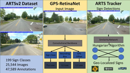
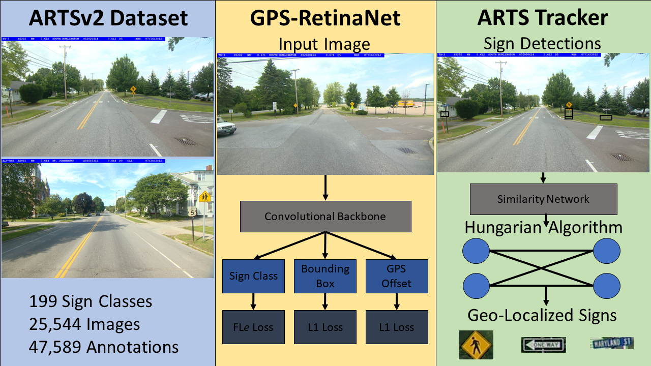
• An enhanced version of the ARTS [9] dataset, ARTSv2, to serve as a benchmark for the field of object geo-localization.
• A novel object geo-localization technique that handles a large number of classes and objects existing in an arbitrary number of frames using only accessible hardware.
• An object tracking system to collapse a set of detections in a noisy, low-frame rate environment into final geo-localized object predictions.

2. Related Work

A somewhat similar area of research are simultaneous localization and mapping (SLAM) algorithms which are designed to model the surrounding environment typically for the purposes for vehicle navigation [10]. By contrast, the purpose of geo-localization algorithms is to determine object positions on a global scale by predicting their GPS coordinates and building a geographical information systems (GIS) map. Furthermore, since SLAM is intended primarily for navigation, these algorithms are designed to run in real time. Object geo-localization algorithms can be applied to pre-existing datasets, since they are not necessarily intended for real time applications.

Object geo-localization from images has been the focus of important recent research. Before deep learning, the most common approach for object geo-localization was to use epipolar constraints [11] to reconstruct 3D points from corresponding image locations. This method has been used to predict traffic light locations [12], and to triangulate and estimate the locations of traffic signs that were detected from their silhouette [13]. A related approach [14] proposed a pipeline that triangulated telecom assets using a histogram of oriented gradients (HOG) as feature descriptors, along with a linear SVM [15] from Google Street View (GSV) images. These methods suffer from poor performance as they used handcrafted features.

Deep neural networks (DNNs) have become the new state-of-the-art technique in geo-localization due to their capabilities to capture complex relationships directly from data through building an effective hierarchical feature representation. While it is already common practice to detect objects in images using deep learning approaches, object geo-localization has the additional requirement that objects appearing in multiple images must be merged into a single prediction. There are three core approaches to accomplishing this merging. First, in triangulation-based approaches, triangulation is used to determine object geo-locations and then a clustering algorithm is typically employed to merge repeated detections [6,7]. The second class of approaches are re-identification-based. In these approaches, a model jointly detects objects using multiple frames as input. When making predictions, these models produce a single prediction for an object from the multiple input frames, thus implicitly merging objects in those frames into a single prediction [2,3]. Third, tracker-based approaches explicitly associate objects between frames, forming tracklets of detections from the same object [1]. These tracklets can then be condensed using a weighted average or a similar approach to create a final sign prediction.

The first triangulation-based approach was proposed by [6], who built a framework that uses a convolutional neural network (CNN) to perform monocular depth estimation from images. They used a Markov random field (MRF) to triangulate the coordinates of the detected objects, and merged the repeated occurrences of objects across multiple images using a clustering algorithm. The authors later expanded their method by incorporating point cloud data captured from drones to enhance geo-localization accuracy [7]. This enhancement came at the cost of introducing a hardware constraint due to requiring drone footage. Triangulation methods are limited in their performance as they rely on noisy segmented objects. Ref. [16] proposed to reduce the noise associated with this method using a structure from motion technique. All these approaches contain the fundamental assumption of object sparsity, in which all objects within a certain distance threshold are assumed to be a single object.

The first re-identification-based method was proposed by [2], who combined object detection and re-identification into a joint learning task using a soft geometric constraint on detected objects from GSV images. The largest limitation of this approach is it required each object to appear in exactly two images, which was not a reasonable real world assumption. To address this limitation the same authors [3] proposed GeoGraph, a graph neural network (GNN)-based method for geo-localization, which is capable of jointly detecting objects in more than two frames. Both these models require a fixed number of input images to be determined before training. Real-world data do not contain objects that disappear after a fixed number of frames, meaning these approaches are not sufficient for real scenarios.

The only tracker-based approach was proposed by [1]. They constructed a deep neural network consisting of an object pose regression network and an object matching network. The object pose regression network detects objects and predicts their 5D pose. The object matching network matches the detected objects to combine objects with repeated appearances in multiple images. The limitation of this approach is that the camera’s intrinsic matrix along with six different image perspectives were used as input to the algorithm, meaning specialized hardware must be used to gather the inputs for the model.

In addition to the drawbacks mentioned for these techniques, most notably, all share a major limitation in which they are only capable of geo-localizing one class of objects. In this paper, we are going to propose a new multi-class tracking-based technique for object geo-localization from images. Our proposed technique can handle objects that might exist in one or multiple frames. Our algorithm uses a single camera, the image’s GPS location, and the image’s heading, which makes our system viable for mass adoption using a cheap hardware.

Many general purpose tracking-by-detection frameworks have been developed over the past decade for a wide range of applications [17,18,19,20,21,22]. The most common approach is to use visual cues and motion tracking to trace objects in a sequence of images [23,24,25,26]. An alternative approach is to train a model to explicitly measure the similarity of each pair of objects. Ref. [27] constructed a deep siamese convolutional network to learn such a similarity function, which was trained during an offline learning phase and then evaluated during tracking. Another approach is to model multiple object tracking using a Markov decision process (MDP), as proposed by [28]. A final noteworthy approach uses dual matching attention networks to incorporate both spatial and temporal information [23]. The networks generate attention maps on input images, which are used to perform tracking.

Most object geo-localization datasets are limited to low frame rates. Traditional object trackers are designed for high frame rate data in which objects only move small distances between frames. They cannot be effectively applied to datasets where there are large jumps between frames. Furthermore, traditional trackers are not designed to take advantage of objects’ GPS coordinates as additional information with which to perform association between frames. We therefore cannot apply traditional object tracking approaches to our dataset, and instead opt to design a novel tracker to address the unique properties of our geo-localization dataset.

3. Datasets

3.1. Existing Datasets

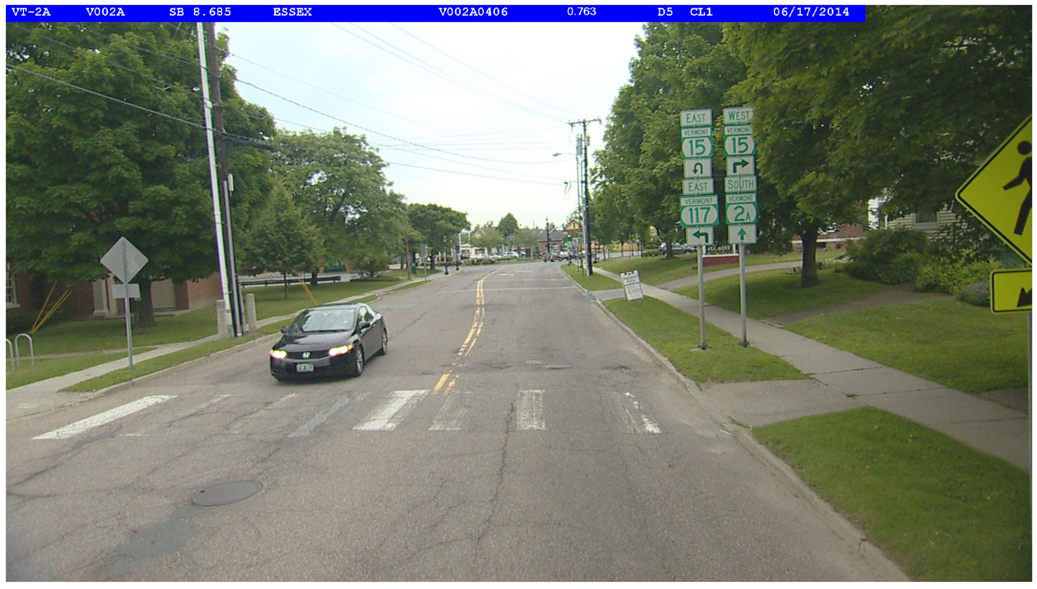
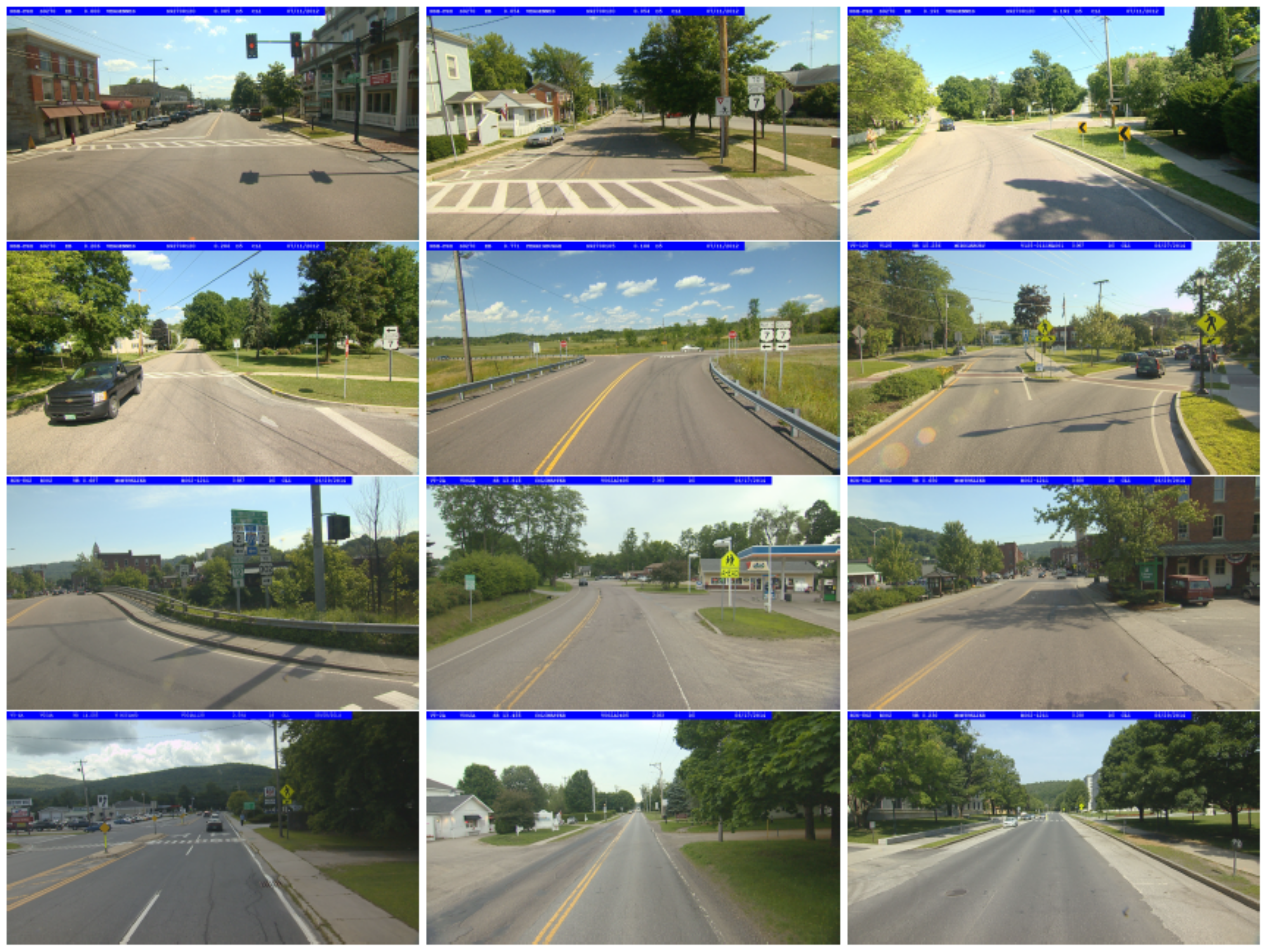
Despite recent interest, only a limited of datasets have been proposed to support research in object geo-localization. There are three major datasets (Pasadena, TLG, and ARTS) which are summarized in

Table 1. A comparison between the Pasadena multi-view object re-identification [2], the traffic light geo-localization (TLG) [1], ARTS v1.0 easy and challenging [9], and ARTSv2.0 datasets.

	Pasadena Multi-View ReID [2]	Traffic Light Geo-Localization (TLG) [1]	ARTS v1.0 [9]		ARTSv2.0
			Easy	Challenging
Number of classes	1	1	78	171	199
Number of images	6141	96,960	9647	19,908	25,544
Number of annotations	25,061	Unknown	16,540	35,970	47,589
Side of the road					🗸
Assembly					🗸
Unique Object IDs	🗸	🗸			🗸
5D Poses		🗸
GPS	🗸	🗸	🗸	🗸	🗸
Color Channels	RGB	RGB	RGB	RGB	RGB
Image Resolution	$2048\times 1024$	$1600\times 1900$	$1920\times 1080$	$1920\times 1080$	$1920\times 1080$
Publicly Available		🗸	🗸	🗸	🗸

.

Ref. [2] proposed a multi-view dataset in which the goal is to re-identify multiple occurrences of street side trees from different views. It includes 6020 individual trees, 6141 GSV images formatted as panoramas, and 25,061 bounding boxes. Each tree was annotated from its four closest panoramas, and is labeled with a unique ID so re-identification can be performed; however, their dataset is not publicly available, and is limited due to not containing distinct classes of objects. It is limited in its size due to only containing 6141 images. This dataset also assumes object sparsity, meaning that all objects within a nearby radius are assumed to be the same object. Furthermore, their dataset does not contain clusters of objects, which is the most challenging scenario for object geo-localization algorithms.

Researchers from Uber [1] compiled another dataset for traffic light detection derived from nuScenes, a popular open-source dataset for autonomous driving [29]. The dataset has 400 scenes, each lasting 20 s with 12 frames per second. All images have metadata indicating the 5D pose of the camera and each annotated traffic light. Each traffic light can be distinguished by a uniquely assigned ID. Their dataset is also limited in that it lacks object classes. It is built from images in a single city-like environment, which lacks the variation associated with data from the real world. Objects are only selected for the dataset if they appear in at least five keyframes. These assumptions artificially reduce the difficulty of the dataset relative to the real world. This dataset is also reliant on the availability of the camera’s intrinsic matrix, which requires the use of specialized hardware to capture.

The third noteworthy dataset was ARTS proposed by [9]. The original ARTS dataset is composed of nearly 20,000 images containing 171 different classes of signs. The dataset is structured as sequences of images referred to as road segments. Each segment contains a sequence of images taken from a camera mounted to the top of a car driving down a road, with roughly one second intervals between each image to satisfy storage constraints. Each image contains an annotation for each readable sign, and each annotation specifies a bounding box around the sign, the sign’s class, and the GPS coordinates of that sign. The camera’s coordinates and heading are also available for each image. The ARTS dataset contains an easy and challenging subset, along with a third format referred to as video logs. All three configurations of the dataset provide manually labeled annotations in a format similar to PASCAL VOC [30]. The easy version of the dataset contains a total of ∼10 K images and ∼17 K annotations, covering 78 different sign classes. All annotated signs in the easy version were captured at up to a 100 m radius of the camera with a minimum of 50 samples per class. The challenging version of the dataset contains a total of ∼35 K annotations scattered in ∼20 K images, covering 171 sign classes, with a minimum of 20 samples per class captured from a distance up to 100 ms. The video logs contain the raw sequences of images and their annotations in the same directory, without being organized into train, validation, and test sets.

The ARTS dataset would benefit from more training samples to address its sparse class distribution by providing more effective samples per class. In addition, a limitation of the ARTS dataset is that it lacks unique identifiers to indicate repeated occurrences of the same sign in multiple images, which inhibits the capability of researchers to benchmark models on this dataset. In the following section, we are going to propose our extension to the ARTS dataset, which will be the largest dataset for traffic sign geo-localization and benchmarking.

3.2. ARTSv2 Dataset

Substantial enhancements have been made to the ARTS dataset [9] to construct ARTSv2. We have increased the number of images to 25,544, the number of unique sign classes to 199, and the number of annotations to 47,589. These enhancements help provide more training samples for less common sign classes, which is one of the fundamental problems with this dataset. Moreover, each sign annotation has been updated with additional attributes. First, each annotation specifies the ‘sign side’, which indicates the side of the road the sign is on, represented as a string indicating left, right, or other. The “other” string is provided for signs that should not be labeled as either left or right, such as signs attached overhangs above the road. Second, each annotation has a binary attribute marking whether the sign is part of an assembly. A sign assembly refers to a group of signs supported by the same post. An example assembly is shown in Figure 1. Each sign that is part of an assembly will have this boolean attribute annotated as True, whereas stand-alone signs that are not part of an assembly will have this attribute set to false. Finally, each physical sign in a road segment has been given unique integer identifier. Since most signs appear in multiple images, a sign annotation will have the same ID each time the that physical sign appears. These unique identifiers are crucial since in order to evaluate the performance of geo-localization algorithms, repeated occurrences of the same object must be identified. Sample images are shown in Figure 2.

All the systems proposed and implemented in this paper use the ARTSv2 dataset.

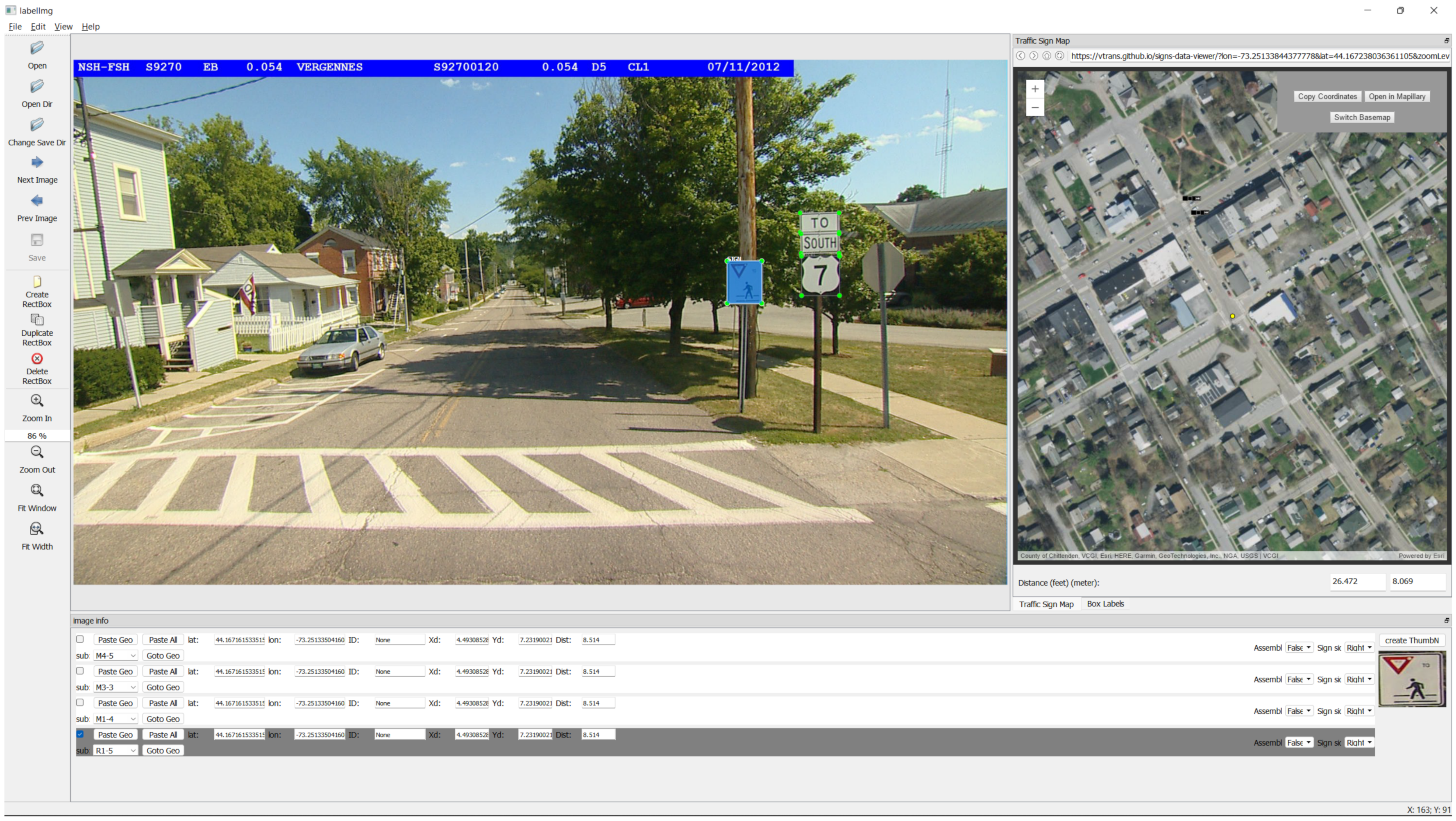
3.3. Dataset Construction

To construct this dataset, images were first gathered from a vehicle with a top-mounted camera, which records footage while traveling in the State of Vermont in the United States. The vehicle travels across the state to capture footage in a wide range of environments, including highways, cities, and rural streets. Since the storage constraints associated with storing so much video would be prohibitive, frames along with their respective GPS and headings are extracted from the video at approximately 1 s intervals. To construct the annotated dataset from these images, human annotators used a version of labelImg [31], which we have modified with the capability to annotate each sign’s GPS coordinates, road side, assembly attribute, and unique integer identifier. This tool will be made publicly available to support the construction of other geo-localization datasets. An image of the user interface is shown in Figure 3.

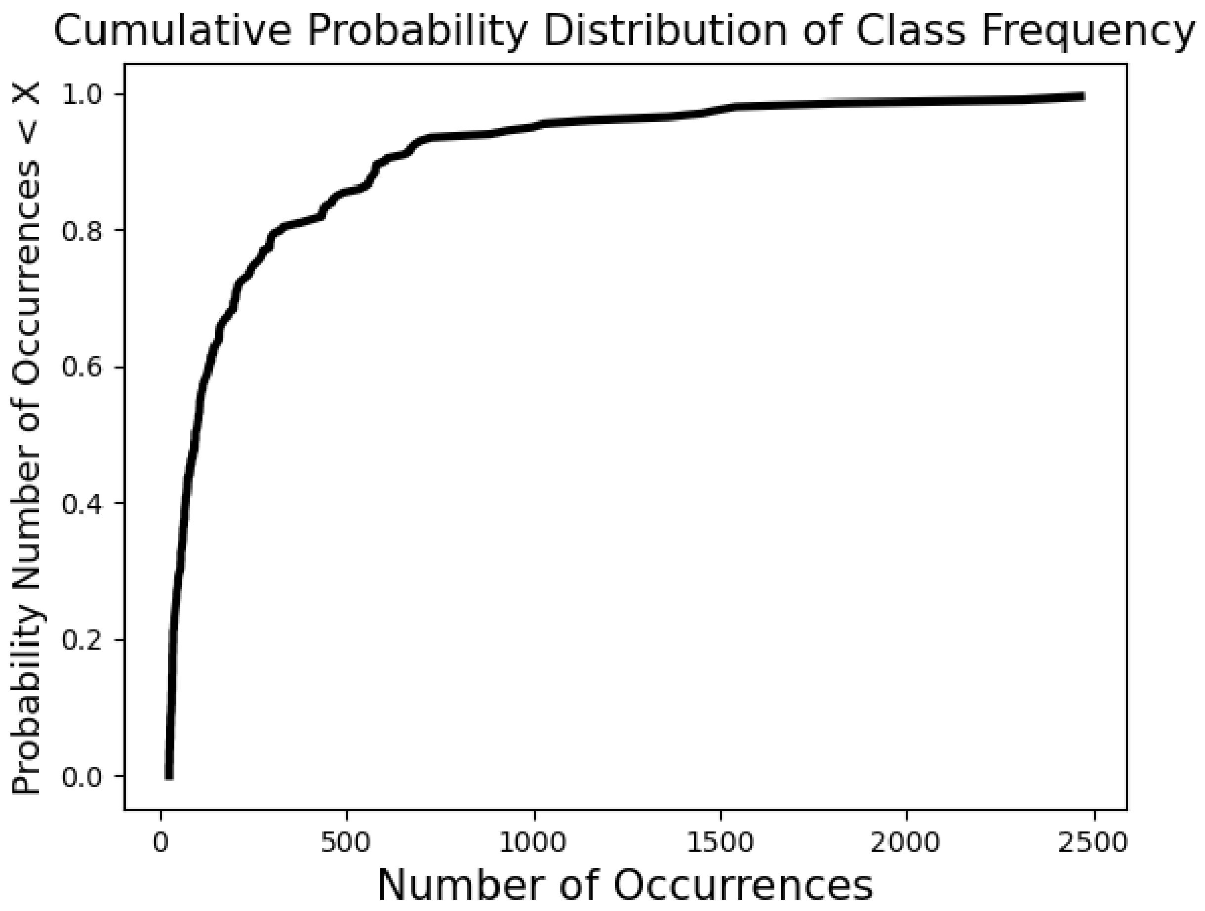
3.4. Unique Characteristics

Compared to other traffic recognition and geo-localization datasets, ARTS is the largest in terms of both the number of images, classes, and annotations. The dataset contains high quality 1920 × 1080 resolution images, available in multiple formats including video logs and individual annotations in a format similar to the PASCAL VOC format. ARTSv2 is also the only dataset containing labels specifying side of road and assembly attributes. Table 1 shows a full comparison between ARTS and similar geo-localization datasets in terms of number of classes, number of images, and number of annotations for each dataset.

Current datasets for object geo-localization algorithms are simple and constructed under ideal circumstances [1,2]. The ARTSv2 dataset contains multiple unique challenges, which makes it more representative of circumstances encountered in the real world. First, ARTSv2 features 199 different sign classes appearing with a highly imbalanced distribution, thereby classes such as stop signs appear far more frequently than more obscure classes of signs. This is an important characteristic of our dataset, since imbalanced class distributions are a substantial challenge currently faced by machine learning models. The heavy-tailed distribution increases the difficulty of training models to predict sign classes appearing less frequently because they have fewer training samples. In addition to posing a significant challenge, this class imbalance is much more representative of what we expect to see in the real world compared to other datasets. This class imbalance is visually illustrated in Figure 4, which shows the cumulative probability distribution of class frequencies in the dataset.

US traffic sign classification also faces the unique challenge of inconsistency between states. While the US Department of Transportation standards are followed to varying degrees, there are a wide variety of specific traffic sign configurations across state road networks. Roads contain many signs that do not conform to known standards. Classifying these non-standard signs therefore poses another unique challenge, as models must learn to cope with signs that may be truly unique, meaning that they only appear once in the entire dataset. Signs that do not fit into a clear category were annotated with an “unknown” class label.

Another unique challenge associated with this dataset is the existence of many objects with similar appearances to road signs, which tends to create false positives from object detectors. Business signs and billboards, hand-made signs placed for events such as yard sales, and car license plates tend to create false positives because they contain visual characteristics similar to road signs. Models trained on this dataset therefore face the challenge of learning to distinguish between road signs, sign-like objects, and other signs that are not technically classified as road signs.

The ARTSv2 dataset was captured in a wide variety of driving environments. There are road segments corresponding to highways, small rural roads, complex intersections, and busy city roads. The vehicle travels at a variety of speeds, takes many turns, and moves up and down hills, which causes signs to change their positions unpredictably between frames. The vehicle may move between other cars or trees such that a sign is visible in one frame and obscured in the next, only to re-appear again a few frames later. Unlike other datasets, we do not remove these non-ideal scenarios since we expect them to be encountered when applying this technology to the real world.

Finally, sign assemblies are a particularly challenging component of our dataset for several reasons. First, assemblies contain clusters of nearby signs that need to be individually detected and geo-localized. Clusters of nearby objects is the most common challenge for object geo-localization algorithms, which is why other datasets have opted to remove them. This challenge is compounded by the fact that signs of similar appearance are particularly likely to occur on the same assembly, since assemblies tend to group together signs intended for a specific function, such as an indicating nearby highways. These assemblies of signs have similar GPS coordinates and often extremely similar appearances, meaning there are few features a model can use to distinguish between these objects. Clusters of similar objects is the most difficult characteristic of the ARTSv2 dataset, which is a challenge that has been neglected by previous research.

4. Materials and Methods

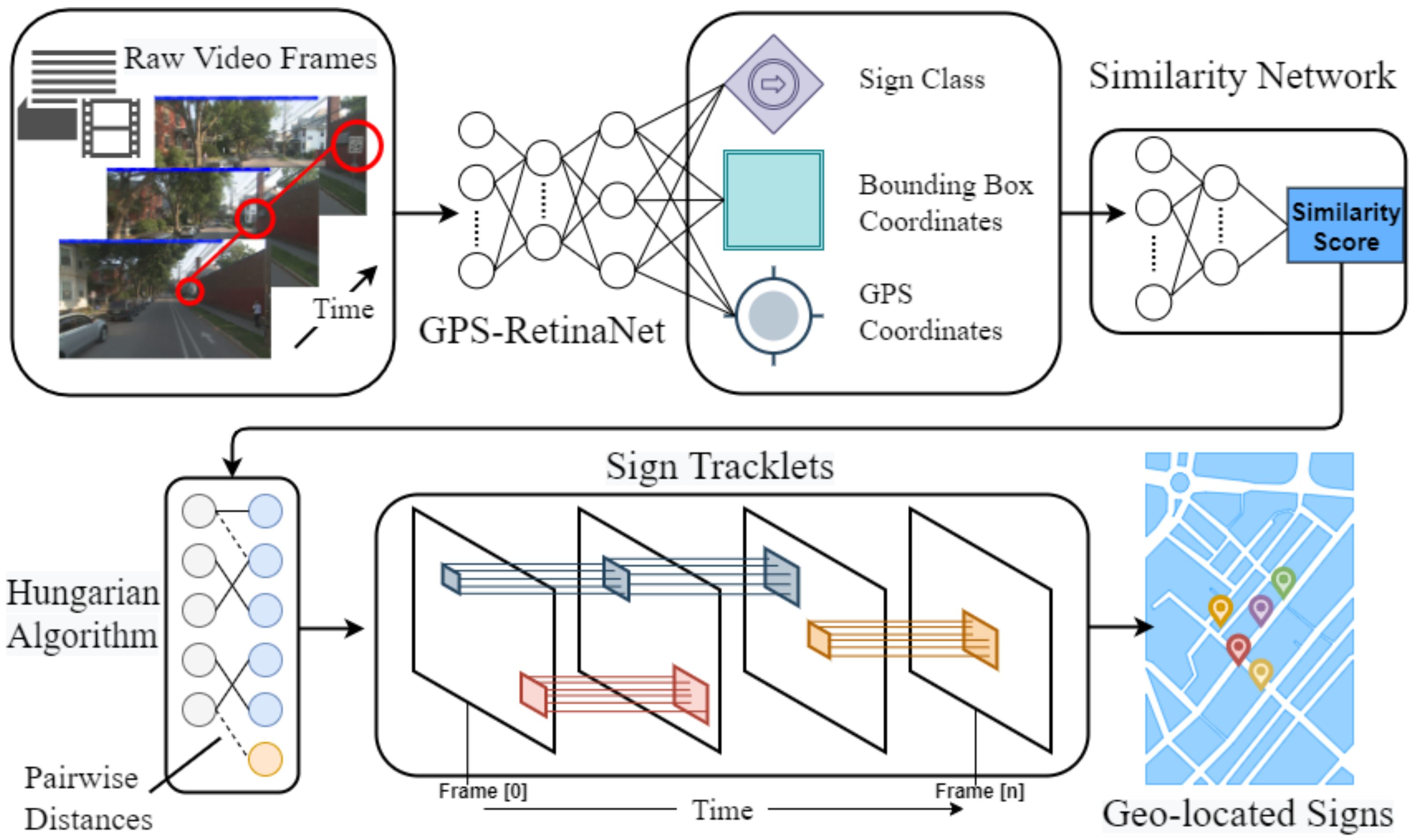
4.1. System Overview

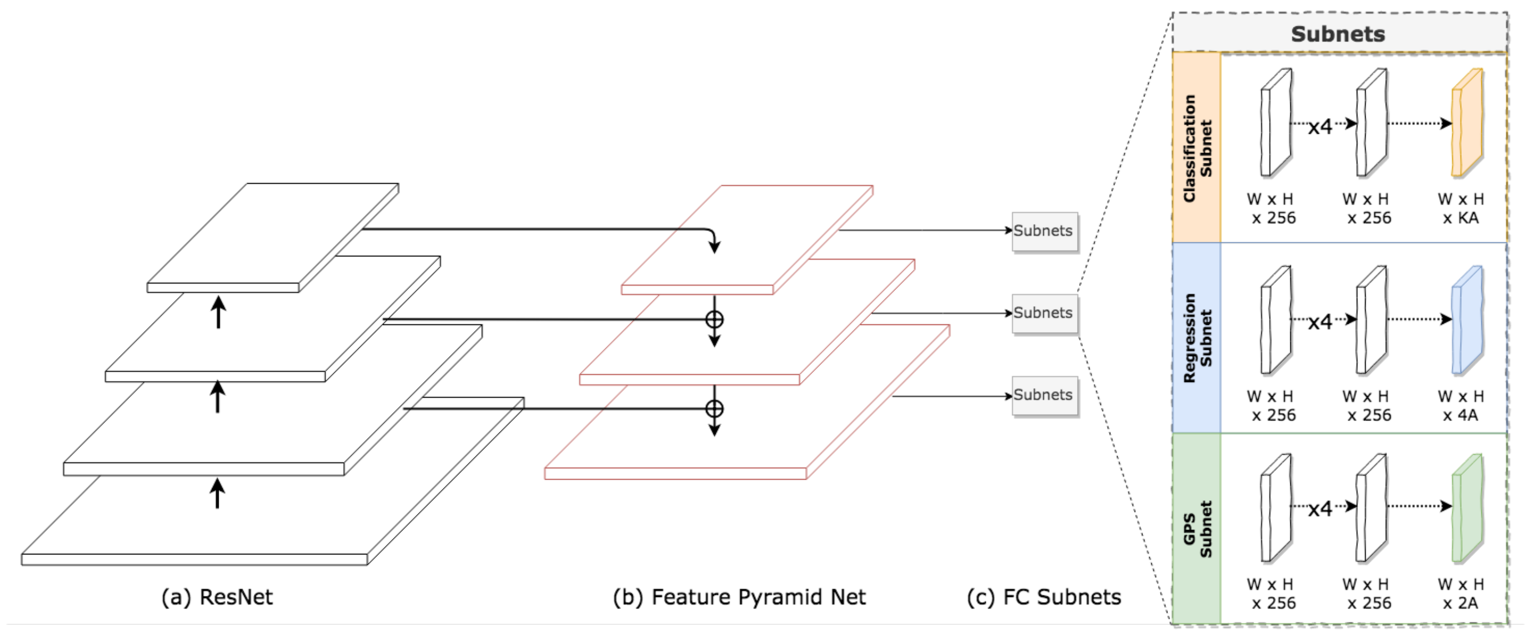
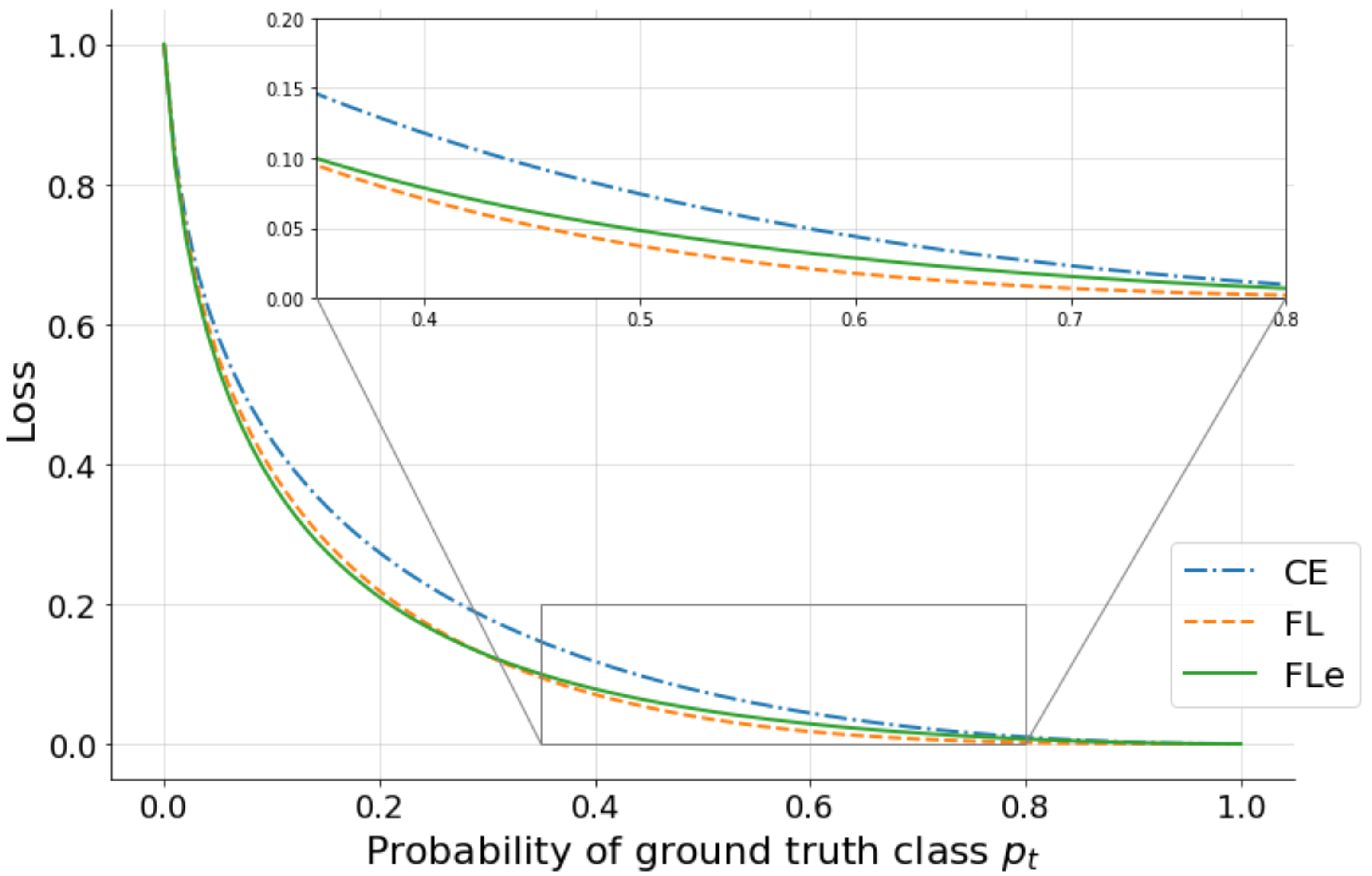
At a high level, our system is composed of two core stages as displayed in Figure 5.

In the first stage, road images are provided to a modified RetinaNet we have constructed called GPS-RetinaNet. GPS-RetinaNet receives these images as input, and outputs a bounding box around each sign, its sign class, and its geospatial location. Since most signs will appear in multiple images, the purpose of the second stage of our system is to condense these repeated detections into a single prediction. First, we train a similarity network, which receives pairs of sign detections predicted by GPS-RetinaNet as input. The similarity network learns to predict a scalar value that measures how similar its input detections are. Next, we used a modified variant of the Hungarian algorithm to pair detections of high similarity. Intuitively, detections with high similarity are more likely to be from the same sign. A list of signs paired together by the Hungarian algorithm is referred to as a tracklet. Each tracklet is then condensed into final sign prediction using a weighted average, producing the final GIS map as shown in Figure 6. The following sections will break the components of this pipeline down in more detail.

4.2. GPS RetinaNet

The first stage of our model performs three functions. It detects each sign visible in a road side image, classifies what type of sign it is, and regresses its geospatial coordinates. We have constructed a system with these capabilities by modifying the popular object detector RetinaNet [21]. RetinaNet is an object detector already capable of performing detection and classification. It uses a backbone network as the core of the architecture, and employs a feature pyramid network to extract features from this backbone. The outputs from the feature pyramid are provided as input to two sub-networks, one of which regresses bounding boxes around objects and the other of which predicts the detected object’s class. RetinaNet is not, however, capable of regressing geo-coordinates. We modified its architecture by building GPS-RetinaNet, which contains an additional fully connected GPS sub-network. The GPS sub-network extracts features from RetinaNet’s feature pyramid [21] and learns to regress a detected object’s offset in a coordinate system local to the image. We call this additional sub-network the GPS subnet, which expands RetinaNet’s base architecture as is displayed in Figure 7. Each sub-network is composed of four fully connected convolutional layers with ReLU activations. The classification sub-network terminates with ($K\times A$) linear outputs, where A is the number of different anchors used in the network and K represents the number of classes. The box-regression sub-network ends with ($4\times A$) linear outputs to determine the relative position of the object [21]. The GPS sub-network concludes with ($2\times A$) linear outputs for each spatial level in the network. We use the popular ResNet [33] as the backbone for this architecture. Sample outputs are shown in Figure 8.

Since directly predicting GPS coordinates of signs is challenging without knowing which direction an image is facing, we instead train the GPS sub-network to predict offsets relative to the image, which we then convert to the sign’s actual GPS coordinates. In more detail, the GPS-subnet learns to regress two local offset values, indicating the horizontal and vertical distance to the sign in meters, which represents the position of the detected object from the perspective of the camera image. These offsets are then fed into a coordinate transform to generate the object’s predicted GPS location as follows:

$$X_r=X_o\times cos\theta +Y_o\times sin\theta$$

(1)

$$Y_r=X_o\times sin\theta -Y_o\times cos\theta$$

(2)

$$O_{lat}=Y_r/6378137$$

(3)

$$O_{lon}=X_r/(6378137\times cos(\pi \times C_{lat}/180))$$

(4)

$$P_{lat}=C_{lat}+O_{lat}\times 180/\pi$$

(5)

$$P_{lon}=C_{lon}+O_{lon}\times 180/\pi$$

(6)

The variables $X_o$ and $Y_o$ represent the respective horizontal and vertical offsets predicted by the network from the perspective of the image in meters. We use $\theta$ to represent the camera’s facing direction (measured with a compass), and $C_{lat}$ and $C_{lon}$ indicate the camera’s latitude and longitude. Both $X_r$ and $Y_r$ are calculated as the meter offsets along the longitudinal and latitudinal axis after being rotated from the camera’s coordinate system. Hence, $O_{lat}$ and $O_{lon}$ are offsets converted from meters to latitude and longitude, and $P_{lat}$ and $P_{lon}$ provide the final latitude and longitude prediction of the detected object after adding the predicted offset of the camera coordinates.

To provide supervision when training the network, we must be able to calculate the desired offsets from the annotated GPS coordinates. In other words, in addition to the capability of converting the offsets predicted by the network to GPS coordinates, we also require the ability to invert this transformation and convert the annotated GPS coordinates to offsets. This can be simply accomplished by re-arranging the above formulas as show below, in which all of the variables remain the same, except that $P_{lat}$ and $P_{lon}$ are replaced with $A_{lat}$ and $A_{lon}$, which represent the annotated latitude and longitude of the sign, respectively.

$$O_{lat}=(A_{lat}-C_{lat})\times \pi /180$$

(7)

$$O_{lon}=(A_{lon}-C_{lon})\times \pi /180$$

(8)

$$X_r=O_{lon}\times (6378137\times cos(\pi \times C_{lat}/180))$$

(9)

$$Y_r=O_{lat}\times 6378137$$

(10)

$$X_o=X_r\times cos\theta +Y_r\times sin\theta$$

(11)

$$Y_o=X_r\times sin\theta -Y_r\times cos\theta$$

(12)

One of the most challenging characteristics of the ARTSv2 dataset is its heavy class imbalance. To address this, we propose a modification to Focal Loss [21] that replaces $\gamma$ in the original definition with an adaptive modulator. We define the new focusing parameter as:

$$\mathrm{\Gamma }=e^{(1-p_t)},$$

(13)

$$\mathrm{F}\mathrm{L}e\left(p_t\right)=-{(1-p_t)}^{\mathrm{\Gamma }}log\left(p_t\right).$$

(14)

For convenience, we refer to our new definition of Focal Loss as (FLe) throughout the paper. FLe introduces two new properties to the original definition. First, it dynamically fine-tunes the exponent based on the given class performance to reduce the relative loss for well-classified classes while maintaining the primary benefit of the original FL. Figure A1 directly compares FL with FLe, highlighting that FLe (shown in green) crosses over $F{L}_{\gamma =2}$ (shown in orange) around ($p_t=0.3$). As $p_t$ goes up from $0.3\to 1$, FLe starts to shift up slowly ranging in between FL and Cross Entropy CE (shown in blue). See Appendix A for more technical details. We use FLe loss to train the classification sub-network, and we use the standard L1 loss to train the bounding box and GPS regression sub-networks.

4.3. Multi-Object Tracker

When GPS-RetinaNet is applied to an image, it produces detections for each sign specifying a bounding box, sign class, and (after a coordinate transform) GPS coordinates. Because images in the ARTSv2 dataset are taken approximately one second apart, the same sign will typically appear in multiple frames. Since our final goal is to produce one geo-localized sign prediction for each sign, we need to collapse the multiple detections produced for many signs into a single prediction for each distinct, physical sign. Our proposed solution is a tracker that iteratively steps through the images in each road segment from the ARTSv2 video logs. As the tracker steps through the images, it merges repeated detections from the same signs appearing in multiple frames. This tracker is composed of two core components, the similarity network and the Hungarian algorithm. The role of the similarity network is to compute a learned heuristic indicating how likely it is a pair of detections provided by GPS-RetinaNet refer to the same sign. The second component, which is a modified variant of the Hungarian algorithm, uses these similarity scores as input to merge repeated detections. Our multi-object tracker is designed to operate in a low-frame rate environment in which objects can move considerable distances along unpredictable trajectories between frames due to the vehicle’s motion. The tracker incorporates both the use of visual cues, predicted GPS position, predicted class, and relative bounding box position to address the core challenge posed by clusters of similar signs.

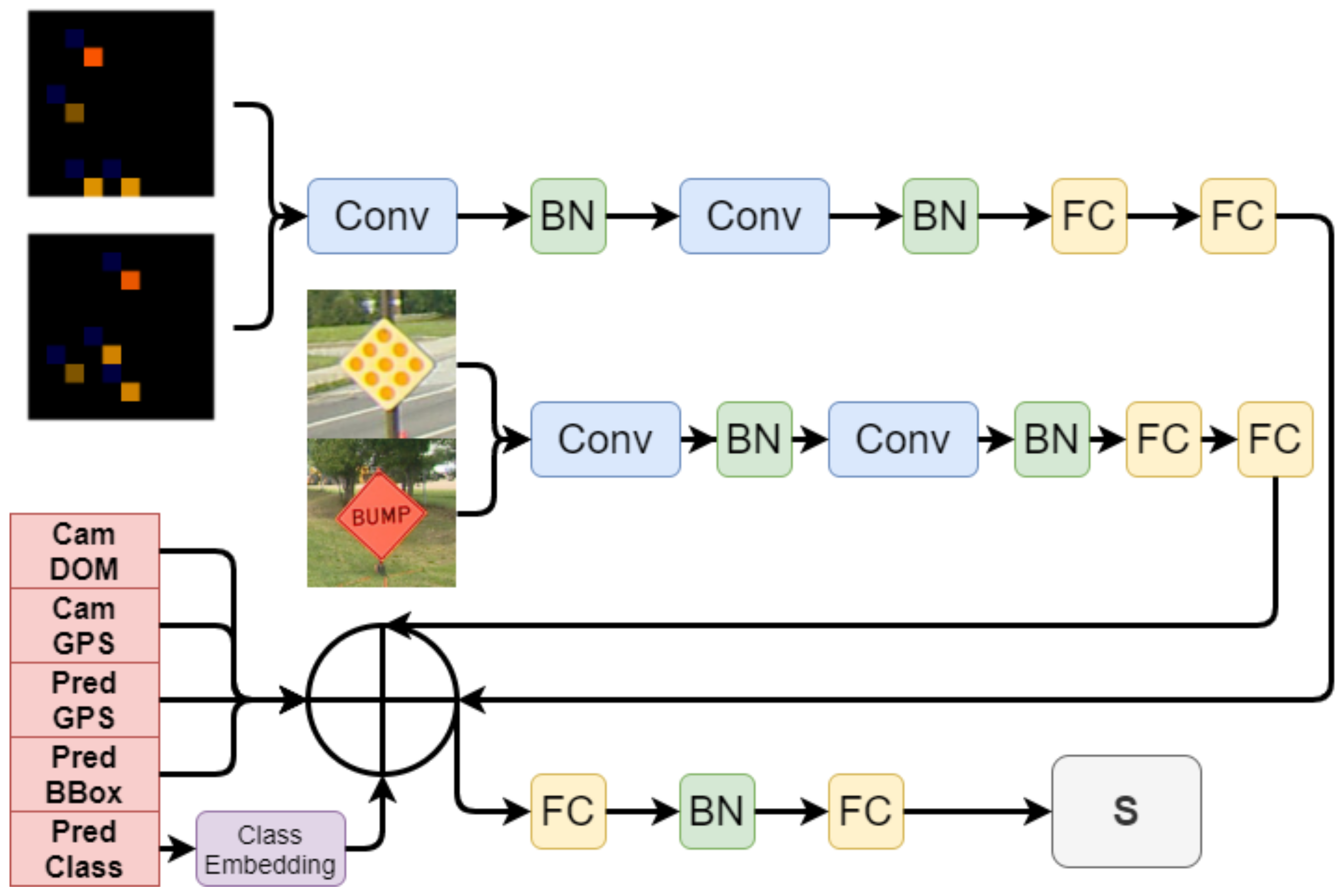
4.3.1. Similarity Network

To train the similarity network, we format the sign annotations from the ARTSv2 dataset to the same format as the detections output by GPS-RetinaNet, so that they can be used as the inputs when training the network. We can use the unique integer identifiers from ARTSv2 to determine if a pair of annotations fed to the similarity network are from the same sign, which will determine the appropriate output for the network during training.

As shown in Figure 9, the similarity network receives three types of inputs associated with each annotation. First, the similarity network receives a vector of values containing the image GPS, image heading, the sign class (represented as a 50 dimensional embedding vector), sign GPS, and bounding box. The second input to the similarity network is the pixels showing an image of the sign. The pixel information within the sign’s bounding box is extracted and resized to a $32\times 32\times 3$ resolution using bi-linear interpolation. The third input to the network is a rank 3 tensor containing a “snapshot” encoding the spatial position of each sign relative to all other signs in the image. This is accomplished by assigning each sign in the frame to a square in a $10\times 10$ grid, corresponding to its location in the image. The correct square to place the sign at is calculated using Equation (15), in which $G_x$ and $G_y$ represent the grid X and Y cells the sign is placed, $B_x$ and $B_y$ indicate the center coordinates of the sign’s bounding box, H and W are the height and width of the image, and S is the size (in our case 10) of the grid. Along the depth axis at each square in grid containing a sign, we concatenate a vector containing that sign’s GPS coordinates and its 50 dimensional class embedding. Grid locations that do not contain a sign are padded with a vector of zeros. The net result is a 3D tensor containing a “snapshot” of information encoding the relative position of signs in the image. This component of our architecture is crucial to address the challenge of signs with similar or identical appearance discussed in Figure 1. If two identical by appearance signs are in an image, this input can allow those signs to be distinguished based on their position in the grid relative to one another. Since the similarity network predicts the similarity of a pair of signs, it receives two instances of each of these three inputs, one of which is from each sign.

$$G_x=\lfloor B_x/W\rfloor \times S$$

(15)

$$G_y=\lfloor B_y/H\rfloor \times S$$

(16)

The network is trained to predict a value between 0 and 1, which represents the probability that a pair of detections belong to the same sign. These values can be interpreted as a similarity metric, where output values closer to 0 indicate the sign detections have greater similarity, and are thus less different from one another. Conversely, when receiving inputs from different signs the network should predict outputs closer to 1, indicating that the detections have less in common with one another.

The architecture of this network contains two siamese sub-networks and a third sub-network designed to handle the remaining inputs. The $32\times 32\times 3$ scaled images containing the pixels from the detections are fed through the first siamese sub-network consisting of two sets of convolutional layers containing 32 $3\times 3$ convolutional filters followed by batch normalization. The resulting features are sent through two fully connected layers resulting in a vector of 32 features. The 3D tensors containing a snapshot of all the signs are processed by a second siamese sub-network consisting of two convolutional layers each containing 32 $3\times 3$ convolutional filters, which are followed by two fully connected layers resulting in a vector of 8 features. The fully connected outputs of these two siamese sub-networks are concatenated with the vector containing the camera heading and GPS, predicted sign GPS, sign class, bounding box, and sign class embedding. The resulting vector is sent through multiple fully connected layers to generate the final prediction. The exact architecture is shown in Figure 9.

The final task of training the similarity network is to develop a satisfactory noise distribution when training. During test time, the similarity network receives output detections from GPS-RetinaNet as input, but as discussed above we must train the similarity network on annotations from our dataset since they contain the labels indicating if two signs are the same. We therefore want to construct a noise distribution for these training annotations that mimics the noise introduced by our object detector. To find a noise distribution, we implemented an algorithm that tests if an annotation has an obvious detector output match when the image that annotations is from is provided as input to GPS-RetinaNet. First, we checked if the annotation’s bounding box has one (and only one) detection in the same image for which their intersection over union (IOU) is greater than 0.9. If this is the case, we measure the latitude and longitude discrepancy between the annotation and detection, create a boolean variable indicating if the classes match, and subtract the differences between the X and Y coordinates of their bounding boxes. These three values quantify how much “noise” was introduced by the detector by measuring how different the annotation is from the corresponding detection predicted by GPS-RetinaNet. By repeating this process for each annotation, we construct a noise distribution representing how often and by how much the detected GPS, detected class, and detected bounding boxes differ from the annotated GPS, annotated class, and annotated bounding box. We can then stochastically sample from this noise distribution to serve as our data augmentation when training the similarity network.

We trained this network on an Nvidia GTX 1080 ti with 11 GB of VRAM and implemented the network using the Keras application programming interface with tensorflow as the back-end. We regularized the inputs from each image such that each color value of each pixel was scaled from 0 to 1. Our network incorporated batch normalization after each layer, in addition to a dropout ratio of 0.25 after each fully connected layer. We fed inputs into the network in batch sizes of 128, and used the Adam optimizer [34] with a learning rate of 0.0001 to optimize the weights of the network. We trained the network for 20 epochs. Finally, since we found categorical cross entropy led to poor performance, we used the mean squared error as the loss function optimize.

4.3.2. Modified Hungarian Algorithm

Once we have learned a function to quantify the similarity between detections, we used the similarity values provided by the network to merge repeated detections from the same signs. We accomplished this with a modified version of the Hungarian algorithm [32]. The Hungarian algorithm provides a polynomial time solution to compute the minimum cost in a bipartite graph where each edge has a matching cost. In each pair of consecutive frames from our dataset, we constructed a bipartite graph where each node represents a detection from that image, and each edge connecting two nodes has a weight that indicates the assignment cost for marking those two nodes as belonging to the same sign. The assignment cost of each pair of signs is determined by providing them as input to the similarity network and taking the resulting similarity score as previously described. By using the Hungarian algorithm to compute the assignments of nodes that achieves the minimum sum of costs, similar sign detections as measured by the similarity network are most likely to be paired, and detections with greater pairing cost are less likely to be paired with one another.

One limitation of the Hungarian algorithm is that it always pairs as many nodes from the bipartite graph as possible. For example, if one set in the graph has 5 nodes and the other set contains 4 nodes, the 4 pairings that minimize the sum of costs will be selected by the Hungarian algorithm. This behavior is undesirable for our application, since it is possible for multiple signs to disappear from view between frames and for many new signs appear to appear in the second frame, so pairing as many nodes as possible would result in nodes representing detections from different objects being incorrectly paired. We solve this problem with a simple modification to the algorithm. If the similarity score computed between a pair of detections is greater than a cutoff threshold of 0.7, then the detected objects are forcibly split, meaning the detections will be placed in separate tracklets. The final output of the tracker is a set of tracklets in which each tracklet represents a list of detections predicted to belong to the same sign.

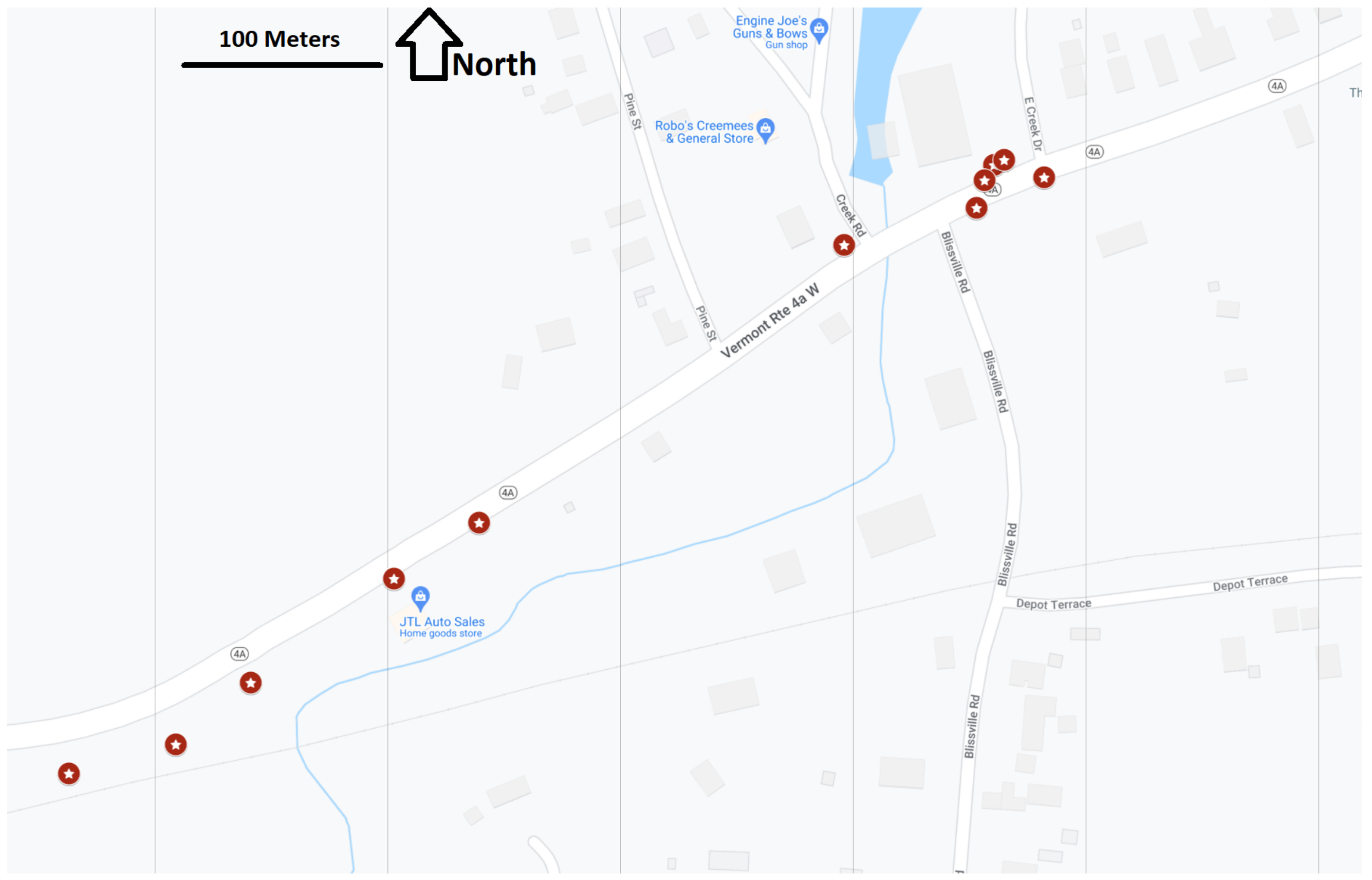
4.3.3. Geo-Localized Sign Prediction

The only remaining step in our pipeline is to condense the tracklets into sign predictions. The simplest method is to predict a sign at the GPS coordinates and with the class from the last frame in the tracklet, which we refer to as the frame of interest (FOI) method. A similarly simple approach is to take a weighted average of the predicted GPS coordinates from each detection in the tracklet. Frames in which the camera is closer to the sign have their predicted GPS weighted more heavily. We predict the class as being the mode of the detections in the tracklet. A third approach involves performing triangulation to condense the tracklets into sign predictions, and predicting the sign class as the mode class from the tracklet. Finally, we can use the Markov random field model proposed in [6] to reduce the tracklets we have produced into sign predictions.

5. Results

5.1. Object Detector Performance

While the ultimate objective of our system is to perform object geo-localization, as an intermediary step we first benchmark the performance of our object detection system. We initialized our object detector with weights from a pre-trained model on the COCO dataset [35]. We kept the default optimization parameters provided by RetinaNet [21] with the exception of increasing the initial learning rate to 1 × 10⁻⁴. We used smooth L1 loss on both the bounding box regression-subnet and the GPS-subnet. The L1 loss for the GPS subnet is computed relative to the correct offset by transforming the annotated GPS coordinates to the local image coordinate system using the transformation outlined in Section 4. We used our custom focal loss function to train the classification subnet. Our models were trained and tested on a workstation with an NVIDIA 1080ti GPU, as well as a computing cluster with NVIDIA Tesla V100 GPUs. We reported the mean average precision mAP evaluated with an intersection over union IoU = 0.5 on the ARTSv2 dataset. To further illustrate the effect of the proposed FLe loss function, we show how the average precision score differs between the worst, 50th percentile, and best performing class. Results are shown in

Table 2. Average precision scores on the testing portion of the ARTSv2 dataset. The MAP score indicates the mean of all average precision scores evaluated at an IoU threshold equal to 0.5. We further show average precision scores for the class with the minimum average precision score, the 50th percentile AP score, and the maximum AP score.

Loss Function	mAP50	APmin	AP50%	APmax
RetinaNet-50 (FL)	69.9	15.9	70.0	100
RetinaNet-50 (FLe)	70.1	17.2	70.1	100

.

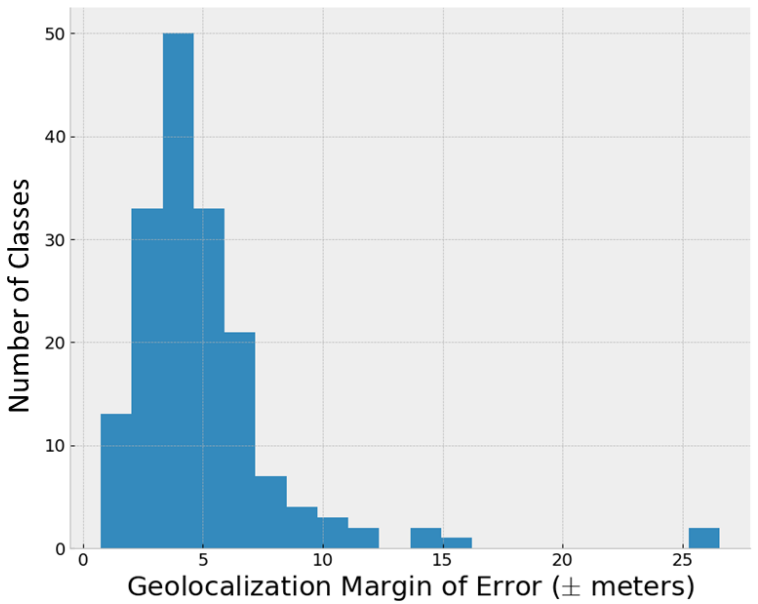
5.2. Object Detector GPS Prediction

Each detection produced by the detector has a corresponding offset prediction from the GPS-subnet, which can be transformed to a GPS location using the previously established coordinate transformation. To quantify the performance of this component of our system, we computed the mean absolute error between the location predicted by GPS-RetinaNet and the ground-truth location of the corresponding sign. To construct an error metric easily interpretable by humans, we converted the absolute error between GPS locations to meters using the Haversine formula, which provides accurate approximations at close distances. The Haversine formula is denoted as follows where $\delta$ is the relative distance, $\psi$ is latitude, $\lambda$ is longitude, and R is the mean of earth’s radius equal to 6371 km:

$$\begin{array}{l}a={sin}^2\left({\displaystyle \frac{\Delta \psi }{2}}\right)+cos{\psi }_1·cos{\psi }_2·{sin}^2\left({\displaystyle \frac{\Delta \lambda }{2}}\right),\\ \delta =2R·atan2\left(\sqrt{a},\sqrt{1-a}\right).\end{array}$$

The distribution of mean GPS regression errors for each class is displayed in Figure 10.

5.3. Similarity Network

Next, we quantified the performance of the similarity network, which learns to predict a value closer to 0 if the two input detections belong to the same physical sign and a value closer to 1 if the detections are from different signs. Intuitively, the range of values from 0 to 1 can be interpreted as an abstract measure of “distance” between the two detections. Values closer to 0 indicate the signs are less distant and thus have more in common, whereas values closer to 1 indicate the signs are more distant and thus less similar. Since this network is not performing classification, we can instead quantify its performance by measuring the absolute error at different percentiles. In

Table 3. A table showing the distribution of prediction errors. Each percentile indicates the percent of absolute errors from the similarity network that are at worst equal to the listed error value.

Percentile	Absolute Error
50	0.0165
75	0.1195
90	0.3846
95	0.6106
97	0.7436
98	0.8064
99	0.8844

, each percentage indicates how often the network predicts a value with an absolute error less than or equal to the listed error value. We use $80\%$ of the annotations for training the network, $10\%$ for validation, and the remaining $10\%$ is reserved for testing.

5.4. Tracker

The objective of the tracker is to collapse down the detections produced by RetinaNet into geo-localized sign predictions. Object geo-localization using deep learning is a new and growing field. There are yet to be any universally accepted performance metrics, especially since performance in this domain is particularly sensitive to the difficulty of the dataset. The goal of our performance evaluation is to quantify how well the physical sign predictions match up with the annotated physical signs distinguished in the ARTS dataset by their integer ID. Specifically, we define a true positive as when the tracker predicts a sign that correctly matches to a real sign within 15 m. We define a false negative as a circumstance where there exists a real sign, but the tracker fails to generate a corresponding prediction. Lastly, we define a false positive to be when the tracker predicts the existence of a sign, but no real-world counterpart exists. An ideal tracker should achieve as many true positives as possible, while minimizing the count of false negatives and false positives.

In

Table 4. A performance benchmark of the full system end-to-end. Raw images are fed into GPS-RetinaNet, which detects signs, predicts their class, and regresses their GPS offsets. Pairs of detections from consecutive frames predicted by GPS-RetinaNet are fed into the similarity network to predict a similarity score. These similarity scores are provided to the Hungarian algorithm to merge repeated detections of the same sign. These final sign predictions are compared to the annotations in the dataset to determine if they are true positives, false negatives, or false positives. The data are organized into three separate years in which it was gathered. Since each year represents a different set of driving environments, the results are shown separately. The 2012 data contain many towns, 2013 contain mostly highways, and 2014 contain a combination of towns are rural segments. The “All” section shows the combined results for all three years.

End-to-End Performance
Year Collected	2012	2013	2014	All
Noteworthy Features	Towns	Highways	Rural Segments and Small Towns	All Geographical Environments
True Positives	264	3170	3179	6163
False Negatives	176	604	842	1622
False Positives	67	826	1581	2474

, we show the number of true positives, false negatives, and false positives during different years containing different road segments. The data for geo-localization are divided into years in which they were gathered, and each year contains road segments that the tracker steps through to perform geo-localization. Each individual year is captured in a variety of geographical regions spread throughout the state of Vermont. Individual years do, however, differ in terms of the driving environments they contain. The 2012 data mostly contain footage from towns, which are challenging due to the density of signs and extra objects present. The 2013 data are composed mostly of highways, and are therefore the least challenging due to having fewer signs, more space between signs, and fewer non-road signs such as signs for businesses. The 2014 data contain many rural segments, which are less challenging, but also contain some towns with difficult sign assemblies.

Figure 11 quantifies the GPS error between each predicted sign and its corresponding ground truth. The x-axis shows the GPS error measured in meters, and y-axis indicates the probability of a sign being geo-localized within the corresponding mean error.

5.5. Comparison to Other Methods

Comparison to existing geo-localization techniques is challenging due to the limitations of current approaches, lack of standardized evaluation metrics and varying structure to datasets.

We believe our dataset is the most representative of data encountered by geo-localization systems in the real world; however, this also limits the comparisons we are capable of performing. For example, it is impossible for us to compare our results to [1], since their method uses 5D pose data, which are unavailable in our dataset. Many other tracking methods do not transfer well to our problem either due to not being designed to deal with the very low frame rate or the broad and sparse class distribution contained by the dataset. Other systems also do not take object class into account, and thus are unable to generate complete predictions on our dataset.

While there are not directly analogous state-of-the-art approaches to compare to, we can compare the geo-localization performance of different techniques on our tracklets. Each algorithm receives as input each sequence of detections created by the tracker, and we will compare how effectively the GPS coordinates of each sign can be determined from each of these tracklets. The simplest method is to predict a sign at the GPS coordinates and the sign’s class using the last detection in the tracklet, which we refer to as the frame of interest method. The intuition behind this approach is the detection should contain the most accurate class and GPS predictions during the last frame in which the camera is closest to the sign. A similarly simple approach is to take a weighted average of the GPS coordinates from the tracklet, in which images where the camera is closer to the sign are weighted more heavily. The class is predicted to be the mode of the detections in the tracklet. Our third approach is to perform triangularization to condense the tracklets into sign predictions. Finally, we use the Markov random field model proposed in [6] to reduce the tracklets into sign predictions. The results are displayed in

Table 5. Performance comparison using different methods to reduce tracklets into sign detections. For each method, we count the total true positives, false negatives, and false postives compared to the ground truth for the full dataset. The mean GPS error indicates the mean absolute distance between a true positive sign prediction and its corresponding ground truth in meters. The STD GPS error indicates the standard deviation of the distribution of true positive GPS errors.

Geo-Localization Performance Comparisons
Tracking Method	True Positives	False Negatives	False Positives	Mean GPS Error	STD GPS Error
Triangularization	6079	3000	1918	6.67	4.33
MRF	6677	4379	2156	6.57	4.98
Frame of Interest	6677	2759	1558	5.85	4.40
Weighted Average	6670	2751	1565	5.81	4.38

.

6. Discussion

6.1. Object Detector Performance

We can see in Table 2 that our proposed FLe loss function slightly improves the average mean average precision score of the object detector. The particular difference between these loss functions, however, is that FLe demonstrated improved tail performance with greater AP scores for more challenging classes. This result supports the effectiveness of FLe in emphasizing low performing classes and ensuring that training gives more weight towards improving their AP. Moreover, FLe does not appear to have significantly decreased the mAP or the AP of classes that performed well with FL. This suggests that FLe is a sound compromise between promoting poorly performing classes and retaining the performance of easier classes.

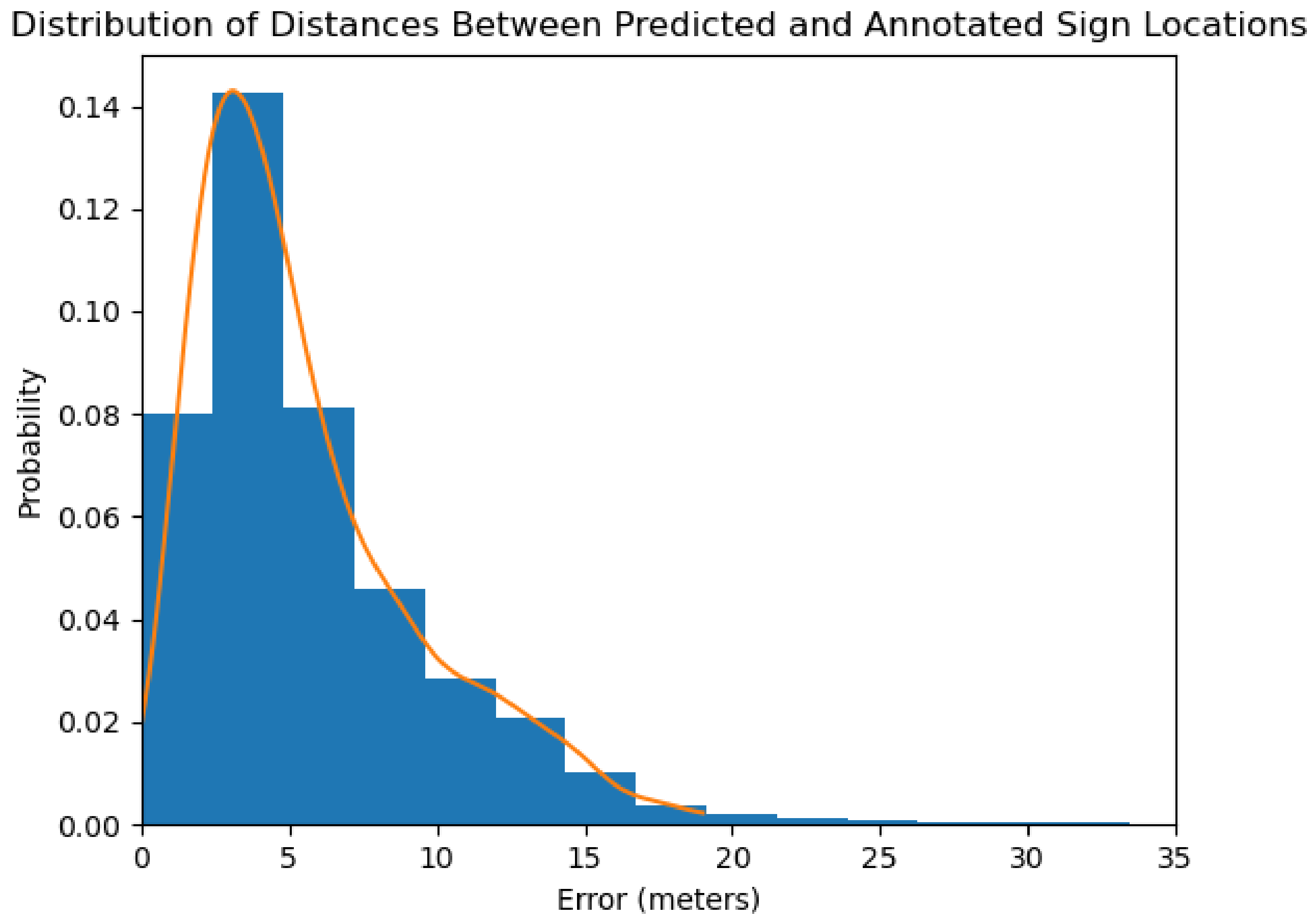
6.2. Object Detector GPS Performance

In Figure 10, we show the distribution of the mean prediction errors for each sign class. We observe that most classes have mean predicted distances within 5 m of their labeled ground truth coordinates; however, we note that it is possible the ground truth coordinates themselves could have additional error due to hardware limitations associated with GPS. We observe that the distribution has a right skew due to a few outlier classes with much larger errors. This is largely a consequence of these signs appearing with low frequency in the dataset. Inspection of these difficult classes revealed they corresponded to signs that have a particularly broad distribution in their size, which is unsurprisingly challenging on a data set composed of images from a single camera.

6.3. Similarity Network

As we can see from Table 3, the similarity network achieved a 90th percentile error of approximately $0.38$. This means that $90\%$ of predictions it made had an absolute error less than or equal to this value. A total of $95\%$ of the prediction errors were less than $0.61$. We can use these values as feedback to decide how we should set our cutoff value for the modified Hungarian algorithm we used. Since we only want to use our cutoff to forcibly split detections when the network is confident they are the not the same sign, this result justifies our decision to use 0.7 as the cutoff threshold.

Visual inspection of failed predictions from the similarity network showed it struggles most with signs that are far away from the camera or similar in appearance to each other. Both these failure cases make intuitive sense because further away and more similar signs will both have fewer visible distinguishing features. Another common failure case for the similarity network is when signs disappear between frames due to being occluded by an object, or are are only partially visible due to being on the edge of the camera’s field of view.

6.4. Tracker

Table 4 shows the final performance results of the full end-to-end system broken down by the different years the images from the dataset are organized into. The performance is strongest for 2013. The images from 2013 are captured from the highway, meaning signs tend to be spread further apart. This means the tracker makes fewer errors in combining detections into tracklets, which results in fewer false positives. By contrast, the 2014 data were captured in a combination of rural environments and towns, and therefore have many sign assemblies containing clusters of similar in appearance signs. This additional challenge resulted in greater false positives due to the previously discussed challenge with differentiating between similar signs within clusters.

Manual inspection of false negatives showed that they typically belonged to small signs that are far away or rotated such that they are not directly facing the camera. Due to their lower visibility, it is unsurprising these characteristics increase the likelihood of a sign being undetected. Inspection of false positives shows many of them are caused by detections of other signs that are not actual road signs. For example, a sign from a restaurant may be detected and predicted as a sign, but since this is not technically a traffic sign it is considered a false positive during evaluation. False positives are also caused by other objects with sign-like appearances such as license plates. Finally, inspection of some false positives revealed they were correct detections of actual traffic signs, however they were not annotated as part of the dataset due to being far off in the background of the image or only partially visible in the frame.

6.5. Comparison to Other Methods

We compared the different methods for condensing tracklets into the final sign prediction as is shown in Table 5. The weighted average approach is the most effective method of converting the tracklets into sign predictions. It achieved the lowest GPS error, low standard deviation, and good scores for true positives, false negatives, and false positives. Using the “Frame of Interest” from each tracklet to create the final sign prediction achieved similar performance. Triangulation has a low standard deviation in its error and is therefore more consistent; however, both triangulation and the MRF approach have greater mean GPS error.

7. Conclusions

In this paper, we presented an enhanced version of the ARTS dataset [9], ARTSv2, which will serve as a comprehensive geo-localization dataset to support future research in the field. Each sign annotation in ARTSv2 consists of a sign class, a side of road indicator, a sign assembly indicator, and a unique sign integer identifier.

We also proposed a novel two-stage object geo-localization system that handles a objects from a large number of heavily skewed classes which exist in an arbitrary number of frames using only accessible hardware. In the first stage, we constructed an object detector called GPS-RetinaNet, which predicts bounding box coordinates, sign classes, and GPS offsets for each detected sign in an input image. GPS-RetinaNet uses FLe, a novel variant of focal loss, during training to effectively handle the class imbalance present in ARTSv2.

The second stage of our proposed modes is a novel object tracking system to collapse a set of detections in a noisy, low-frame rate environment into final geo-localized object predictions. The traffic sign tracking and geo-localization was handled using a learned metric network and a variant of the Hungarian algorithm.

Future research should explore optimizations and tuning to facilitate high frame rate object geo-localization.

The noise introduced to GPS coordinates due to both equipment error and annotation inconsistencies limits the capability of GPS to serve as a ground truth. To limit GPS error, future work could use satellite images to achieve enhanced geo-localization performance. Future work could also experiment with how to better distinguish between signs with similar visual features and locations during tracking, as these objects have the fewest distinguishing features.

References

1. Chaabane, M.; Gueguen, L.; Trabelsi, A.; Beveridge, R.; O’Hara, S. End-to-End Learning Improves Static Object Geo-Localization From Video. In Proceedings of the IEEE/CVF Winter Conference on Applications of Computer Vision (WACV), Virtual, 5–9 January 2021; pp. 2063–2072. [Google Scholar]
2. Nassar, A.S.; Lefèvre, S.; Wegner, J.D. Simultaneous multi-view instance detection with learned geometric soft-constraints. In Proceedings of the IEEE/CVF International Conference on Computer Vision, Seoul, Korea, 27 October–2 November 2019; pp. 6559–6568. [Google Scholar]
3. Nassar, A.S.; D’Aronco, S.; Lefèvre, S.; Wegner, J.D. GeoGraph: Graph-Based Multi-view Object Detection with Geometric Cues End-to-End. In Proceedings of the European Conference on Computer Vision, Glasgow, UK, 23–28 August 2020; pp. 488–504. [Google Scholar]
4. McManus, C.; Churchill, W.; Maddern, W.; Stewart, A.D.; Newman, P. Shady dealings: Robust, long-term visual localisation using illumination invariance. In Proceedings of the Institute of Electrical and Electronics Engineers (IEEE) International Conference on Robotics and Automation (ICRA), Hong Kong, China, 31 May–7 June 2014; pp. 901–906. [Google Scholar] [CrossRef]
5. Suenderhauf, N.; Shirazi, S.; Jacobson, A.; Dayoub, F.; Pepperell, E.; Upcroft, B.; Milford, M. Place recognition with ConvNet landmarks: Viewpoint-robust, condition-robust, training-free. In Proceedings of the Robotics: Science and Systems XI, Rome, Italy, 13–17 July 2015; pp. 1–10. [Google Scholar]
6. Krylov, V.A.; Kenny, E.; Dahyot, R. Automatic Discovery and Geotagging of Objects from Street View Imagery. Remote Sens. 2018, 10, 661. [Google Scholar] [CrossRef] [Green Version]
7. Krylov, V.A.; Dahyot, R. Object geolocation using mrf based multi-sensor fusion. In Proceedings of the 2018 25th IEEE International Conference on Image Processing (ICIP), Athens, Greece, 7–10 October 2018; pp. 2745–2749. [Google Scholar]
8. Wilson, D.; Zhang, X.; Sultani, W.; Wshah, S. Visual and Object Geo-localization: A Comprehensive Survey. arXiv 2021, arXiv:2112.15202. [Google Scholar]
9. Almutairy, F.; Alshaabi, T.; Nelson, J.; Wshah, S. ARTS: Automotive Repository of Traffic Signs for the United States. IEEE Trans. Intell. Transp. Syst. 2019, 22, 457–465. [Google Scholar] [CrossRef]
10. Bailey, T.; Durrant-Whyte, H. Simultaneous localization and mapping (SLAM): Part II. IEEE Robot. Autom. Mag. 2006, 13, 108–117. [Google Scholar] [CrossRef] [Green Version]
11. Szeliski, R. Computer Vision: Algorithms and Applications; Springer Science & Business Media: Berlin/Heidelberg, Germany, 2010; pp. 307–312. [Google Scholar]
12. Fairfield, N.; Urmson, C. Traffic light mapping and detection. In Proceedings of the 2011 IEEE International Conference on Robotics and Automation, Shanghai, China, 9–13 May 2011; pp. 5421–5426. [Google Scholar]
13. Soheilian, B.; Paparoditis, N.; Vallet, B. Detection and 3D reconstruction of traffic signs from multiple view color images. ISPRS J. Photogramm. Remote Sens. 2013, 77, 1–20. [Google Scholar] [CrossRef]
14. Hebbalaguppe, R.; Garg, G.; Hassan, E.; Ghosh, H.; Verma, A. Telecom Inventory management via object recognition and localisation on Google Street View Images. In Proceedings of the 2017 IEEE Winter Conference on Applications of Computer Vision (WACV), Santa Rosa, CA, USA, 24–31 March 2017; pp. 725–733. [Google Scholar]
15. Dalal, N.; Triggs, B. Histograms of oriented gradients for human detection. In Proceedings of the 2005 IEEE Computer Society Conference on Computer Vision and Pattern Recognition (CVPR’05), San Diego, CA, USA, 21–23 September 2005; Volume 1, pp. 886–893. [Google Scholar]
16. Liu, C.J.; Ulicny, M.; Manzke, M.; Dahyot, R. Context Aware Object Geotagging. arXiv 2021, arXiv:2108.06302. [Google Scholar]
17. Lin, T.; Dollar, P.; Girshick, R.; He, K.; Hariharan, B.; Belongie, S. Feature Pyramid Networks for Object Detection. In Proceedings of the 2017 IEEE Conference on Computer Vision and Pattern Recognition (CVPR), Honolulu, HI, USA, 21–26 July 2017; pp. 936–944. [Google Scholar] [CrossRef] [Green Version]
18. Girshick, R.; Donahue, J.; Darrell, T.; Malik, J. Rich feature hierarchies for accurate object detection and semantic segmentation. In Proceedings of the IEEE Conference on Computer Vision and Pattern Recognition, Columbus, OH, USA, 23–28 June 2014; pp. 580–587. [Google Scholar]
19. Girshick, R. Fast R-CNN Object detection with Caffe. In Proceedings of the 2015 IEEE International Conference on Computer Vision (ICCV), Santiago, Chile, 7–13 December 2015; pp. 1440–1448. [Google Scholar] [CrossRef]
20. Ren, S.; He, K.; Girshick, R.; Sun, J. Faster R-CNN: Towards real-time object detection with region proposal networks. In Proceedings of the Advances in Neural Information Processing Systems, Montreal, QC, Canada, 7–12 December 2015; pp. 91–99. [Google Scholar]
21. Lin, T.; Goyal, P.; Girshick, R.B.; He, K.; Dollár, P. Focal Loss for Dense Object Detection. arXiv 2018, arXiv:1708.02002. [Google Scholar]
22. He, K.; Gkioxari, G.; Dollár, P.; Girshick, R. Mask R-CNN. In Proceedings of the 2017 IEEE International Conference on Computer Vision (ICCV), Venice, Italy, 22–29 October 2017; pp. 2980–2988. [Google Scholar]
23. Zhu, J.; Yang, H.; Liu, N.; Kim, M.; Zhang, W.; Yang, M.H. Online multi-object tracking with dual matching attention networks. In Proceedings of the European Conference on Computer Vision (ECCV), Munich, Germany, 8–14 September 2018; pp. 366–382. [Google Scholar]
24. Voigtlaender, P.; Krause, M.; Osep, A.; Luiten, J.; Sekar, B.B.G.; Geiger, A.; Leibe, B. Mots: Multi-object tracking and segmentation. In Proceedings of the IEEE/CVF Conference on Computer Vision and Pattern Recognition, Long Beach, CA, USA, 15–20 June 2019; pp. 7942–7951. [Google Scholar]
25. Son, J.; Baek, M.; Cho, M.; Han, B. Multi-object tracking with quadruplet convolutional neural networks. In Proceedings of the IEEE Conference on Computer Vision and Pattern Recognition, Honolulu, HI, USA, 21–26 July 2017; pp. 5620–5629. [Google Scholar]
26. Xu, J.; Cao, Y.; Zhang, Z.; Hu, H. Spatial-temporal relation networks for multi-object tracking. In Proceedings of the IEEE/CVF International Conference on Computer Vision, Seoul, Korea, 27 October–2 November 2019; pp. 3988–3998. [Google Scholar]
27. Bertinetto, L.; Valmadre, J.; Henriques, J.F.; Vedaldi, A.; Torr, P.H.S. Fully-Convolutional Siamese Networks for Object Tracking. In Proceedings of the Computer Vision—ECCV 2016 Workshops, Amsterdam, The Netherlands, 11–14 October 2016; Hua, G., Jégou, H., Eds.; Springer International Publishing: Cham, Switzerland, 2016; pp. 850–865. [Google Scholar]
28. Xiang, Y.; Alahi, A.; Savarese, S. Learning to Track: Online Multi-object Tracking by Decision Making. In Proceedings of the 2015 IEEE International Conference on Computer Vision (ICCV), Santiago, Chile, 7–13 December 2015; pp. 4705–4713. [Google Scholar] [CrossRef] [Green Version]
29. Caesar, H.; Bankiti, V.; Lang, A.H.; Vora, S.; Liong, V.E.; Xu, Q.; Krishnan, A.; Pan, Y.; Baldan, G.; Beijbom, O. nuScenes: A multimodal dataset for autonomous driving. In Proceedings of the IEEE/CVF Conference on Computer Vision and Pattern Recognition, Seattle, WA, USA, 14–19 June 2020; pp. 11621–11631. [Google Scholar]
30. Everingham, M.; Van Gool, L.; Williams, C.K.I.; Winn, J.; Zisserman, A. The Pascal Visual Object Classes (VOC) Challenge. Int. J. Comput. Vis. 2010, 88, 303–338. [Google Scholar] [CrossRef] [Green Version]
31. Tzutalin. Tzutalin. LabelImg. Git Code. 2015. Available online: https://github.com/tzutalin/labelImg (accessed on 5 April 2022).
32. Kuhn, H.W. The Hungarian Method For The Assignment Problem. Nav. Res. Logist. Q. 1955, 2, 83–97. [Google Scholar] [CrossRef] [Green Version]
33. He, K.; Zhang, X.; Ren, S.; Sun, J. Deep Residual Learning for Image Recognition. In Proceedings of the 2016 IEEE Conference on Computer Vision and Pattern Recognition (CVPR), Las Vegas, NV, USA, 27–30 June 2016; pp. 770–778. [Google Scholar] [CrossRef] [Green Version]
34. Kingma, D.P.; Ba, J. Adam: A Method for Stochastic Optimization. arXiv 2015, arXiv:1412.6980. [Google Scholar]
35. Lin, T.; Maire, M.; Belongie, S.J.; Bourdev, L.D.; Girshick, R.B.; Hays, J.; Perona, P.; Ramanan, D.; Dollár, P.; Zitnick, C.L. Microsoft COCO: Common Objects in Context. arXiv 2014, arXiv:1405.0312. [Google Scholar]
36. Grabner, H.; Grabner, M.; Bischof, H. Real-Time Tracking via On-line Boosting. In Proceedings of the British Machine Vision Conference 2006, Edinburgh, UK, 4–7 September 2006; Volume 1, pp. 47–56. [Google Scholar] [CrossRef] [Green Version]
37. Babenko, B.; Yang, M.H.; Belongie, S. Visual tracking with online Multiple Instance Learning. In Proceedings of the 2009 IEEE Conference on Computer Vision and Pattern Recognition, Miami, FL, USA, 20–25 June 2009; pp. 983–990. [Google Scholar] [CrossRef]
38. Henriques, J.F.; Caseiro, R.; Martins, P.; Batista, J. High-Speed Tracking with Kernelized Correlation Filters. IEEE Trans. Pattern Anal. Mach. Intell. 2015, 37, 583–596. [Google Scholar] [CrossRef] [Green Version]
39. Kalal, Z.; Mikolajczyk, K.; Matas, J. Tracking-Learning-Detection. IEEE Trans. Pattern Anal. Mach. Intell. 2012, 34, 1409–1422. [Google Scholar] [CrossRef] [Green Version]
40. Kalal, Z.; Mikolajczyk, K.; Matas, J. Forward-Backward Error: Automatic Detection of Tracking Failures. In Proceedings of the 2010 20th International Conference on Pattern Recognition, Istanbul, Turkey, 23–26 August 2010; pp. 2756–2759. [Google Scholar] [CrossRef] [Green Version]
41. Held, D.; Thrun, S.; Savarese, S. Learning to Track at 100 FPS with Deep Regression Networks. arXiv 2016, arXiv:1604.01802. [Google Scholar]
42. Bolme, D.; Beveridge, J.; Draper, B.; Lui, Y. Visual object tracking using adaptive correlation filters. In Proceedings of the 2010 IEEE Computer Society Conference on Computer Vision and Pattern Recognition, San Francisco, CA, USA, 13–18 June 2010; pp. 2544–2550. [Google Scholar] [CrossRef]
43. Lukežič, A.; Vojíř, T.; Čehovin Zajc, L.; Matas, J.; Kristan, M. Discriminative Correlation Filter with Channel and Spatial Reliability. Int. J. Comput. Vis. 2018, 126, 671–688. [Google Scholar] [CrossRef] [Green Version]
Figure 1. An example of a sign assembly containing multiple signs of similar appearance. All of the signs on the assembly have a green and white appearance, so it is difficult for a model to distinguish between them. There are two signs containing the word “East” which appear essentially identical. There are also two signs with the text “Vermont 15”. The arrow in the bottom left is a mirrored version of the arrow in the middle right. Since these signs contain so many similar characteristics, and in some cases are nearly identical, it is extremely challenging to create a geo-localization model that separately geo-localizes these signs.
Remotesensing 14 02575 g001
Figure 2. Sample images from the ARTSv2 dataset. The images contain a variety of sign types, often clustered very close together, which makes for challenging geo-localization. Environment and road types also vary widely.
Remotesensing 14 02575 g002
Figure 3. A sample image of the graphical user interface provided by our modified version on labelImg. The image being annotated is displayed in the upper left, and bounding boxes that have been annotated are overlaid on the image. The user can use the map displayed in the upper right to select the GPS coordinates for each sign. In the bottom pane, the user can enter all appropriate information associated with the sign, including its class, GPS coordinates, assembly attribute, sign side, and integer identifier.
Remotesensing 14 02575 g003
Figure 4. A cumulative class distribution plot showing the distribution of frequencies at which different classes appear in ARTSv2. The x-axis indicates a class frequency, and the y-axis value indicates the probability that a class occurs at most the number of times indicated on the x-axis. The sharp rise on the left side of the graph shows there are many classes that appear with low frequency, posing a unique challenge for geo-localization algorithms, which must adapt to classes with few training samples.
Remotesensing 14 02575 g004
Figure 5. An overview of the Sign Hunter pipeline. First, raw images extracted from videos of a road vehicle (top-left) are fed into GPS-RetinaNet (top-middle) which detects, classifies, and predicts signs’ GPS offsets. Pairs of detections output by GPS-RetinaNet are provided as input to the similarity network (top-right), which quantifies the similarity between the signs. The Hungarian algorithm [32] (bottom-left) uses the similarity scores to merge repeated occurrences of objects, which forms tracklets (bottom-middle) containing all the occurrences of each object in the dataset. These tracklets are condensed into final sign predictions to create a GIS map (bottom-right) of sign locations.
Remotesensing 14 02575 g005
Figure 6. The end result of our pipeline is that signs are classified based on their sign type and placed on a map corresponding to their geo-location. Each dot indicates the location of a single sign after all the repeated detections have been merged. Properties of the sign such as its class can be inspected by clicking on it on the map tool.
Remotesensing 14 02575 g006
Figure 7. GPS-RetinaNet. Similar to RetinaNet [21], this architecture uses a FPN [17] backbone on top of a ResNet [33] model (a) to create a convolutional feature pyramid (b). Then, we attach three sub-networks (c); one for classification, one for box regression, and one for GPS/depth regression.
Remotesensing 14 02575 g007
Figure 8. Sample images and detections from the ARTSv2 datset. Images contain a variety of sign types, often clustered very close together, which makes for challenging geo-localization. Each box around each sign represents a separate detection from GPS-RetinaNet. The color of the box represents which tracklet the detection has been assigned to by the multi-object tracker. Since a tracklet is a list of signs predicted to be the same, re-occurrences of the same sign in multiple images should have the same color box around it.
Remotesensing 14 02575 g008
Figure 9. The architecture of the similarity network. The network uses two siamese sub-networks and then concatenates all the resulting features. The remaining features are sent through two more fully connected layers before predicting the similarity score.
Remotesensing 14 02575 g009
Figure 10. Average GPS testing error for each class. The x-axis shows the average geo-localization margin of error of a given class, and the y-axis indicates how many classes fell within that approximate margin of error. Our GPS-subnet scored a median MOE of ( ± 5 ) meters. We can see that the GPS-subnet can accurately estimate distance within a reasonably low margin of error, especially considering how far many signs are from the camera in the ARTSv2 dataset.
Remotesensing 14 02575 g010
Figure 11. A probability distribution of GPS errors between the predicted geo-localized sign coordinates and the actual coordinates from the annotations. The x-axis indicates the amount of GPS error in meters between a predicted and an actual sign, and the y-axis indicates the probability of a random sign having the error indicated on the x-axis.
Remotesensing 14 02575 g011