Article

Drone-Sensed and Sap Flux-Derived Leaf Phenology in a Cool Temperate Deciduous Forest: A Tree-Level Comparison of 17 Species

1
The United Graduate School of Agricultural Science, Gifu University, 1-1 Yanagido, Gifu 501-1193, Japan
2
School of Life Sciences and Technology, Institut Teknologi Bandung, Jl. Ganesa 10, Bandung 40132, Indonesia
3
Faculty of Agriculture, Shizuoka University, 836 Ohya, Suruga-ku, Shizuoka 422-8017, Japan
*
Author to whom correspondence should be addressed.
Remote Sens. 2022, 14(10), 2505; https://doi.org/10.3390/rs14102505
Submission received: 15 April 2022 / Revised: 20 May 2022 / Accepted: 21 May 2022 / Published: 23 May 2022
(This article belongs to the Special Issue Hyperspectral Remote Sensing of Vegetation Functions)

Abstract

:
Understanding the relationship between leaf phenology and physiological properties has important implications for improving ecosystem models of biogeochemical cycling. However, previous studies have investigated such relationships only at the ecosystem level, limiting the biological interpretation and application of the observed relationships due to the complex vegetation structure of forest ecosystems. Additionally, studies focusing on transpiration are generally limited compared to those on photosynthesis. Thus, we investigated the relationship between stem sap flux density (SFD) and crown leaf phenology at the individual tree level using the heat dissipation method, unmanned aerial vehicle (UAV)-based observation, and ground-based visual observation across 17 species in a cool temperate forest in Japan, and assessed the potential of UAV-derived phenological metrics to track individual tree-level sap flow phenology. We computed five leaf phenological metrics (four from UAV imagery and one from ground observations) and evaluated the consistency of seasonality between the phenological metrics and SFD using Bayesian modelling. Although seasonal trajectories of the leaf phenological metrics differed markedly among the species, the daytime total SFD (SFDday) estimated by the phenological metrics was significantly correlated with the measured ones across the species, irrespective of the type of metric. Crown leaf cover derived from ground observations (CLCground) showed the highest ability to predict SFDday, suggesting that the seasonality of leaf amount rather than leaf color plays a predominant role in sap flow phenology in this ecosystem. Among the UAV metrics, Hue had a superior ability to predict SFDday compared with the other metrics because it showed seasonality similar to CLCground. However, all leaf phenological metrics showed earlier spring increases than did sap flow in more than half of the individuals. Our study revealed that UAV metrics could be used as predictors of sap flow phenology for deciduous species in cool, temperate forests. However, for a more accurate prediction, phenological metrics representing the spring development of sap flow must be explored.

Graphical Abstract

1. Introduction

Leaf phenology is the study of annually recurring biological events in plant leaves, such as budburst, development, and senescence, which are tightly linked to plant productivity and water use, especially in deciduous tree species. Leaf phenology is highly sensitive to changes in climatic conditions, particularly air temperature [1,2]. For example, field and remote sensing evidence, predominantly from northern hemisphere regions, shows that a warming climate has advanced the timing of leaf-out and prolonged the growing season in the last half-century [3,4], which may alter the seasonal cycle of ecosystem CO2 fluxes and energy balance [5]. However, when predicting such impacts on biogeochemical cycling with dynamic vegetation and ecosystem process models, leaf phenology is one of the most difficult processes for parameterizing such models because the mechanism behind leaf phenology and its response to environmental drivers are complex [6,7,8]. In this context, simultaneous observation of leaf phenology and physiological functions in forest ecosystems provides important implications for improving the parameterization and structure of such process-based models and, thus, our understanding of how plant communities and terrestrial ecosystems respond to climate change [9].
Leaf phenology has traditionally been evaluated using ground-based visual observations. However, this method is labor intensive, prone to human error, and difficult to apply to trees in dense and multi-layered forests wherein an observer cannot see the entire canopy. Consequently, remote sensing approaches using satellite and tower-mounted digital cameras have become popular for monitoring leaf phenology in forest ecosystems because they enable continuous monitoring of leaf phenology due to fixed viewing geometry and allow objective evaluation of leaf phenology using the reflectance data of acquired images. Especially, a tower-mounted digital camera called a “phenocam”, which is categorized as a near-surface remote sensing approach, can provide ecosystem-level leaf phenology at a higher temporal frequency and finer spatial resolution than satellite remote sensing without being obscured by clouds, enabling detailed comparison of leaf phenology with ecosystem carbon and water flux obtained by the eddy covariance method [10,11]. Because canopy color derived from phenocam imagery depends on both the leaf amount and the color of individual leaves, it reflects both physiological and structural characteristics of the canopy, such as leaf area index (LAI), leaf chlorophyll and carotenoid concentrations [12,13,14,15,16,17], which are key components of canopy photosynthesis and transpiration. Therefore, phenocams have been installed in many flux sites in various ecosystems, such as temperate and boreal forests, savannas, and grasslands, and time-series data of canopy greenness or redness have been used to analyze seasonal changes in ecosystem gas flux, especially for CO2, e.g., [9,10,18,19,20,21].
Although several studies have reported tight correlations between phenocam-derived color metrics and gross primary production (GPP) across seasons in temperate deciduous forest ecosystems, e.g., [22,23,24], many others found large discrepancies between GPP and phenological metrics, especially for the pattern within the growing season; that is, phenocam-derived metrics tend to result in both earlier spring peak and later onset of autumn decrease compared to canopy photosynthesis [9,13,14,18]. Although mid-growing season phenology has received less attention than phenology at the beginning and end of the growing season, it determines the attainment of full photosynthetic capacity and its period, thus affecting the annual sums of GPP. Many possible explanations for the dissimilarity have been inferred, for example, earlier saturation of green signal at relatively low LAI [13], slower development of leaf physiological properties than leaf area [18], spring increase in leaf carotenoid content and subsequent decrease in the fraction of green signal from the canopy, [14] and earlier decrease in leaf physiological properties than the onset of leaf fall, e.g., [25]. However, it is difficult to clarify the cause of these discrepancies from ecosystem-level studies because the observed patterns and relationships between flux and leaf phenology integrate the responses of multiple species, age classes, and canopy layers within the ecosystem; thus, biological interpretation of these relationships is far from trivial. Additionally, phenocam tends to overrepresent dominant trees located closest to the field of view, which causes a footprint mismatch between the flux and optical measurements, especially in species-rich forests with complex structures, leading to errors in the flux–leaf phenology relationship [26]. Consequently, it is difficult to apply the flux–leaf phenology relationship obtained at the ecosystem level to other sites, even in the same biome. In this context, identifying the flux–leaf phenology relationship at the individual tree level is an important step for disentangling the cause of dissimilarity in the ecosystem-level relationship.
Drones, also referred to as unmanned aerial vehicles (UAVs), are other near-surface remote sensing tools that have been increasingly used to monitor leaf phenology [27,28]. Although the temporal resolution of the acquired images is lower than that of phenocams, UAV can produce aerial images at the same spatial resolution as phenocams and cover vast areas, ranging from hectares to multiple square kilometers. This enables the identification and analysis of an extensive number of individual crowns across seasons and years, with the same spatial standard. With respect to flux measurement at the tree level, there is no suitable approach for linking CO2 flux measurement to UAV-derived phenology because tree-level CO2 flux measurement requires enclosing the entire crown with a gas exchange chamber, impeding UAV observation [29]. In contrast, stem sap flow measurements using heat dissipation probes can provide a time series of tree-level transpiration data on an hourly to daily scale without enclosing the crown with the chamber, and thus can be directly linked to UAV observation. Additionally, the sap flow sensor is simple to construct, easy to install, and inexpensive compared with other approaches, such as the whole tree chamber, enabling us to measure multiple trees for examining inter- and intra-species variations in flux–leaf phenology relationships. Furthermore, although transpiration is an important factor influencing latent heat flux and photosynthesis, previous studies have primarily focused on the relationship between leaf phenology and canopy photosynthesis but not transpiration, probably because the H2O flux obtained by the eddy covariance method encompasses processes other than transpiration, such as evaporation of soil water, canopy intercepted water, and other free water surfaces, which do not directly correlate with leaf phenology. Although fundamental factors controlling tree transpiration (i.e., amount of leaf area and leaf physiological properties) are similar to those controlling photosynthesis, leaf water-use efficiency (i.e., the ratio of photosynthesis to transpiration) is not constant across seasons [30,31]. Thus, we expected that leaf phenological metrics related to transpiration would differ from those related to photosynthesis. Furthermore, because the spatial scales of stem sap flow and UAV-derived crown leaf phenology are identical at the tree level, we can expect closer correlations between sap flow and UAV-derived phenology than the flux–leaf phenology relationships observed at the ecosystem level. However, to the best of our knowledge, no study has identified the relationship between sap flow and camera-derived leaf phenology at the individual tree level in temperate deciduous species.
The main objective of this study was to assess the potential of UAV-derived leaf phenological metrics for tracking the seasonal dynamics of sap flow (i.e., sap flow phenology) at the individual tree level across multiple species. To achieve this objective, we examined seasonal changes in crown colors using UAV imagery, in conjunction with stem sap flow measurements using the thermal dissipation method, for 17 deciduous broad-leaved species in cool temperate forests for two years (2019–2020). We also monitored crown leaf cover using ground-based visual observations to evaluate the contribution of changes in leaf amount to sap flow phenology. Additionally, because sap flow is sensitive to day-to-day fluctuations in environmental factors (unlike leaf phenology), we used a Bayesian model driven by phenological metrics and environmental factors to compare sap flow and leaf phenology directly.

2. Materials and Methods

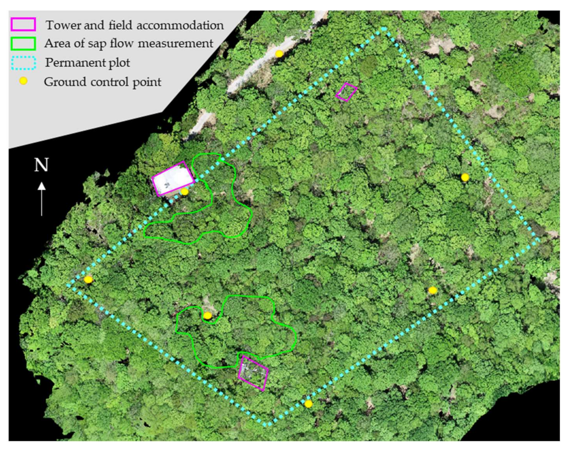
2.1. Study Site and Samples

This study was conducted in a 1.5 ha permanent plot in a cool temperate forest on the eastern side of Mt. Sobatsubu in Shizuoka Prefecture, Japan (35°8′2.5″N, 138°2′43.1″E; 1400 m above sea level, Figure A1). The mean temperature and average annual precipitation for the study years (2019–2020) were 9.7 °C and 3262.5 mm, respectively (precipitation data were obtained from records at the Kawanehoncho meteorological station, provided by the Japan Meteorological Agency; http://www.jma.go.jp/jma/index.html, accessed on 31 March 2022). The plot comprised 43 tree species, including 1100 trees with a diameter at breast height greater than 5 cm. The canopy trees had an average height of approximately 18 m, a total basal area of 51.3 m2 ha−1, and a stand leaf area index of 4.1 m2 m−2. The study plot faced southeast and had moderate relief, with slopes most frequently between 10 and 30%. The canopy and sub-canopy layers (ca. > 15 m and 5–15 m, respectively) were predominated by Acer shirasawanum Koidz. (40.2% of the total basal area); other overstory tree species included Fagus crenata Blume (7.4%), Betula grossa Siebold & Zucc. (5.7%), Fraxinus spp. (5.6%), and Acer nipponicum H.Hara (4.5%). The understory vegetation (<5 m) was substantially less than that expected under normal conditions because of continuous excessive browsing by Sika deer since 2007 and mass flowering and die-off events of dwarf bamboo (Sasa borealis (Hack.) Makino & Shibata) in 2016. Although the study plot was surrounded by a fence in 2016, the vegetation had not recovered completely. Two canopy access towers, 15–20 m in height, were established in the plot (Figure A1), and standard micrometeorological conditions, such as radiation, temperature, humidity, and wind speed, were continuously monitored from April to December at the top of one of the two towers located in the southern part of the plot. Electric power for all types of sensors and dataloggers was provided by solar panels mounted on the south tower and the roof of a field accommodation adjacent to the plot.
During the two consecutive years (2019 and 2020), we chose 29 canopy trees belonging to 17 species (Table 1, Figure A1). Because the UAV approach is prone to be affected by below-crown vegetation, such as understory vegetation, sub-canopy trees, and branches of neighboring trees, we selected target trees with small below-crown vegetation as much as possible, especially for species showing later bud break. Additionally, to minimize errors in ground visual observation, we selected trees for which the entire crown was visible from the ground through gaps around the trees. We changed the sample trees by year, except for the four trees that were continually measured for two years, because suitable tree samples could not be found within 25 m (limit of cable length for sap flow measurement) from the solar panels. Consequently, we obtained data from 33 individuals in total.

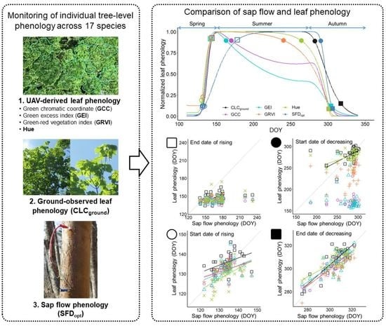
2.2. Observation of Leaf Phenology

Leaf phenology of the sampled tree crown was monitored using ground-based visual observations and UAV observations conducted on the same day from late April to mid-November at a weekly to biweekly frequency, depending on weather conditions. Measurements were taken on 21 and 24 distinct occasions in 2019 and 2020, respectively (Table A1).
With respect to ground-based visual observation, the observer looked at the target crowns from various directions using binoculars and estimated the percentage of unfolded leaves and the mean leaf size as the percentage of mature leaf size. Photographs of the target crown were also taken on each occasion to check the accuracy of the mean leaf size derived from visual observations. Crown leaf cover (CLCground) was then calculated as a product of the percentages of unfolded leaves and leaf size, and the result was categorized into one of the seven classes as follows: 0%, 10% (1–19%), 30% (20–39%), 50% (40–59%), 70% (60–79%), 90% (80–99%), and 100% (Figure S3 in the supplementary materials of [28]). Ground observations were performed by the same person throughout the seasons to minimize any errors associated with different observers. Because changes in leaf color were not considered in the evaluation of CLCground, CLCground represents changes in the relative amount of leaf area. A preliminary experiment showed that CLCground was closely correlated with the effective plant area index derived from hemispherical photographs (Figure A2). Further details of ground-based visual observation are described in the paper by Budianti et al. [28].
For UAV observations, aerial photographs were taken using a commercial drone (DJI Phantom 4 pro, DJI-Innovations Inc., Shenzhen, China) equipped with an RGB camera (DJI FC6310) with an 8.8 mm nominal focal length and a 1” CMOS 20-megapixel sensor with 2.41 × 2.41 µm nominal pixel size. Prior to each UAV flight, the camera was configured for continuous shooting with the following settings: infinity focus, ISO 800, and exposure time of 1/1000 s. The photographs were stored in JPEG format with super-fine compression. Although a clear day was chosen to conduct UAV flights based on the weather forecast, weather conditions at the study site were generally unstable due to rapidly changing regional weather conditions (i.e., fog and cloud). Therefore, the UAV was manually operated to change flight plan flexibly according to the weather conditions. To ensure sufficient overlap of images to produce an orthophoto (80% longitudinal and 50% lateral overlap [33]), the UAV was operated at roughly 1.2 m s−1, with the camera taking images every 2 s, and at least five flights were conducted over the 1.5 ha plot (25 min per flight). The flight height was 35–45 m above the ground (i.e., 15–20 m above the crown surface of sample trees). To minimize the effect of variable illumination on the UAV image due to the solar incidence angle, the flights were conducted at midday (between 10:00 and 14:00) on most occasions, whereas variable illumination conditions during flight inevitably occurred on some occasions due to the unstable weather conditions at the study site (Table A1).
Each acquired image set was processed into a georeferenced orthophoto using the Context Capture software (Bentley Systems Inc., Exton, PA, USA). Although the entire image processing (i.e., bundle adjustment and reconstruction of three-dimensional model) was performed nearly automatically by the software [33], seven ground control points in the plot, determined using a global navigation satellite system with a precision of less than several centimeters (Figure A1), were included in the process to refine georeferencing. Additionally, to mitigate the negative effect of unsteady illumination conditions on orthophoto production, a color equalization algorithm was used in the software, which ensures consistent appearance of the acquired images even under largely different illumination conditions. Orthophotos were successfully produced at the centimeter resolution, except for three occasions in November 2019 when orthophotos could not be produced owing to mechanical trouble with the UAV camera (Table A1).

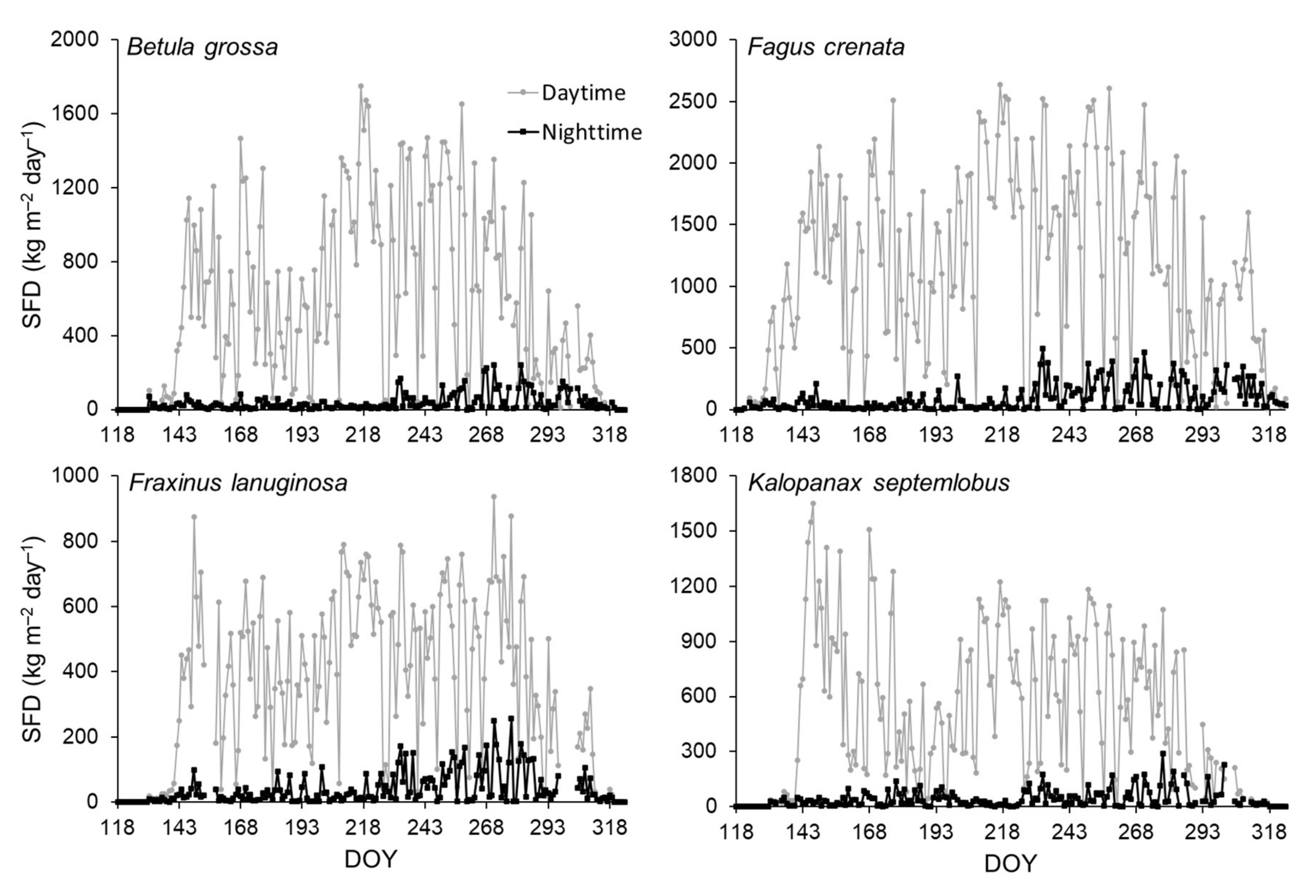
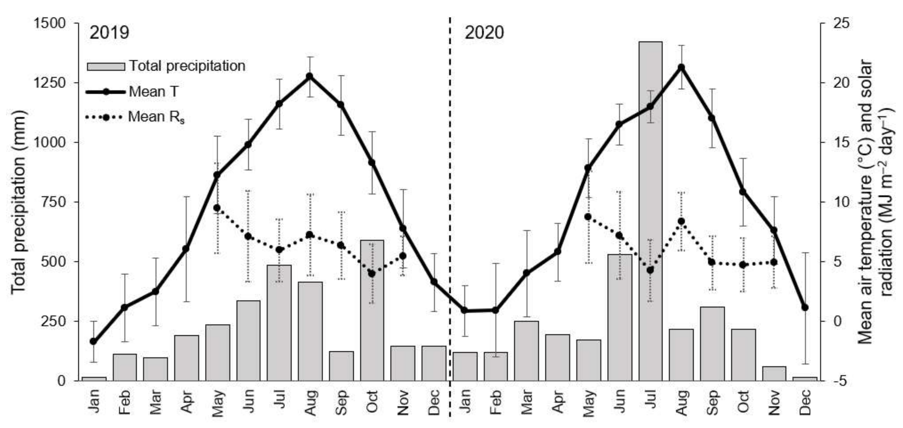
2.3. Measurements of Sap Flow and Environmental Factors

Sap flux density (SFD) of the tree stems was measured with the thermal dissipation method using self-made Granier-type sensors [34] installed 1.5 m above the ground. Each sensor consisted of two probes (2 cm long and 2 mm in diameter). The upper probe included a heater supplied with 0.2 W constant power. The heat was dissipated into the sapwood and provided an estimate of the vertical sap flux surrounding the probe. For each sample tree, one sensor was installed at 0–2 cm depth in the sapwood, with the two probes separated by 15 cm. All sensors were installed on the north side of the stem and covered by a shelter of reflective insulation to avoid thermal disturbance by radiation, wind, and rainfall. Each tree was continuously monitored from mid-April (before bud break) to the end of November (after all the leaves had fallen) at 30 sec intervals, and 30 min averaged data were recorded on a data logger (CR1000, Campbell Scientific, Logan, UT, USA) with a peripheral multiplexer (AM16/32, Campbell Scientific, Logan, UT, USA). However, occasionally, data loss occurred due to equipment failure caused by frequent lightning and animal attacks and also due to power supply problems during prolonged rainy days in July and September (Figure A3). The recorded temperature difference between the two probes was converted into the SFD, as described by Granier [34]. The highest temperature difference (ΔTmax) was defined as the zero-flux condition for each day. The ΔTmax values determined for each day were generally similar throughout the experimental period (data not shown).
Solar radiation above the canopy was measured using a solar radiometer (LI-200, Li-Cor, Lincoln, NE, USA), and air temperature and humidity in the canopy layer were measured using a thermohydrograph (CS215, Campbell Scientific Inc., Logan, UT, USA). Meteorological data were sampled and recorded at the same frequency as the sap flow measurements and on the same data logger. The vapor pressure deficit (VPD), calculated from the temperature and relative humidity using the Tetens formula [35], was also recorded on the data logger using a customized logging program written in CRBasic (Campbell Scientific Inc., Logan, UT, USA).

2.4. Data Analysis

2.4.1. UAV-Derived Leaf Phenological Metrics

We manually delineated the boundaries of the 29 target crowns (i.e., the regions of interest) in orthophotos based on the ground survey and calculated four phenological metrics for the delineated crown space using ArcGIS software (version 10.7, ESRI, Redlands, CA, USA) as follows:
GCC = G/(R + G + B)
GEI = 2G − (R + B)
GRVI = (G − R)/(G + R)
Hue = (G − B)/(DNmax − DNmin) × 60, if R = DNmax
Hue = (B − R)/(DNmax − DNmin) × 60 + 120, if G = DNmax
Hue = (R − G)/(DNmax − DNmin) × 60 + 240, if B = DNmax
where GCC, GEI, and GRVI are green chromatic coordinate, green excess index, and green-red vegetation index, respectively. R, G, and B are the mean values of the red, green, and blue digital numbers, respectively, in the target crown space. DNmin and DNmax are the minimum and maximum digital numbers (DN) of the RGB channels, respectively. To compare the four metrics on the same scale, all the metrics were normalized from 0 to 1 using the minimum and maximum values of these metrics over seasons.
For the three occasions in November 2019 when orthophoto construction failed, the phenological metrics were calculated directly from the aerial JPEG images that had a similar perspective to the orthophotos. Additionally, although we chose sample trees with small below-crown vegetation as much as possible, significant influence of the below-crown vegetation on the start dates of the spring rising phase was found for five of the 29 trees. In that case, we removed the influence by post-processing the orthophotos, for example, by adjusting the size of the region of interest and/or exchanging the below-crown vegetation image with the adjacent ground image.

2.4.2. Calculation and Normalization of Daytime Total Sap Flow

To characterize the seasonal dynamics of sap flow (i.e., sap flow phenology), the daytime total SFD (SFDday) was calculated for each sample tree by summing the SFD values from 5:00 to 20:00. Although nighttime SFD is generally marginal, we excluded it from our analysis because nighttime SFD gradually increased from summer to autumn in response to nighttime VPD for more than half of the individuals (Figure A4), complicating the model for the environmental response of SDF (Equation (6) in the next subsection). The SFDday of the individual trees was also normalized from 0 to 1 in the same manner as that used for the phenological metrics. Normalization allowed us to compare seasonal dynamics and environmental responses between trees with different absolute magnitudes. Although exploration of phenological metrics reflecting absolute SFDday is also an important challenge, quantification of absolute SFD values requires calibration of sap flow sensors by destructive tree sampling and investigation of spatiotemporal variations in SFD within the stem [36,37,38], which was difficult to achieve because of legal restrictions on tree harvesting and limited equipment. Therefore, a comparison of the UAV metrics and absolute SFD was beyond the scope of this study.

2.4.3. Modelling the Phenology of Sap Flow

Wullschleger et al. [39] described the seasonal dynamics of sap flow in temperate deciduous tree species using the following empirical function:
SFD = FLAI·(a·Rs + b·VPD)
where FLAI is the normalized leaf area index (LAI), Rs is the solar radiation (MJ m−2 day−1), VPD is the vapor pressure deficit (hPa), and a and b are coefficients. To evaluate the potential of the leaf phenological metrics for predicting sap flow phenology, we replaced FLAI of Equation (5) with normalized leaf phenological metrics (PMnorm), and adapted the hierarchical Bayesian framework as follows:
SFDday t = PMnorm t·(at·Rs_day + bt·VPDday)
where Rs_day and VPDday are the daily total Rs and the daytime mean VPD, respectively. The subscript of each variable and coefficient, i.e., t, refers to an individual tree. Additionally, to determine the phenological transition dates of sap flow, we estimated the seasonal dynamics of PMnorm using the double logistic model given by Gu et al. [40]:
PMnorm t = c1t/[1 + exp {−(TtT1t)/d1t}]e1tc2t/[1 + exp {−(TtT2t)/d2t}]e2t
where T is the day of the year, and c1, c2, d1, d2, e1, e2, T1, and T2 are coefficients. Because PMnorm is estimated from the measured SFDday and environmental factors using Equations (6) and (7), we referred to it as optimized SFD (SFDopt). The SFDday values estimated by SFDopt were closely correlated with the measured values across all individuals (r2 = 0.89 and root-mean-square error, RMSE = 0.093 for all pooled data, data not shown).
All coefficients were interconnected in this model framework and obtained as probability distributions (i.e., posterior distributions) at the individual tree level. Sampling from the posterior distributions of all parameters was performed using the Markov chain Monte Carlo (MCMC) method. We ran 20,000 iterations for each of the three independent MCMC chains after a warm-up of 12,000 iterations, with the chains thinned every five iterations to yield a posterior sample size of 4800. The convergence of the Markov chains for each parameter was checked using R-hat values (<1.1) by comparing the variance within and among chains. The Bayesian framework and related analyses were run in R version 4.1.2 using the ‘rstan’ package [41].

2.4.4. Calculation of Phenological Transition Dates

To determine the phenological transition dates of the leaf phenological metrics, five double logistic models included in the R package ‘phenopix’ [42] were applied to the time-series data of the phenological metrics, and the best-fitted result was selected based on the RMSE (Figure A5). We then defined the days representing 10%, 50%, and 90% of the maximum amplitude of the fitted results during spring green-up phase as the start, middle, and end dates of the rising phase, respectively (i.e., SOR, MOR, and EOR, respectively). In addition, for the decreasing phase after spring peak, we defined the days that represented 90%, 50%, and 10% of the maximum amplitude as the start, middle, and end dates of the decreasing phase, respectively (i.e., SOD, MOD, and EOD, respectively). The transition dates of SFDopt were defined in the same manner.

3. Results

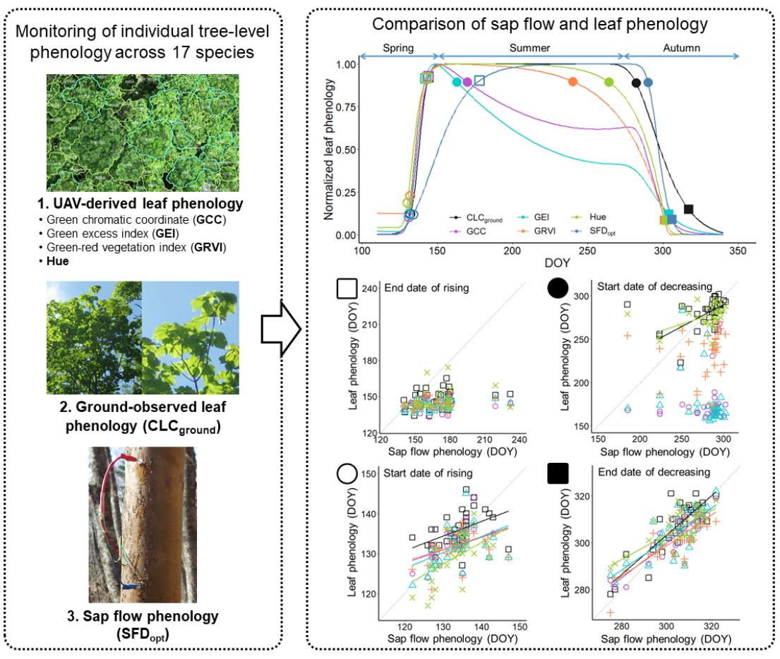
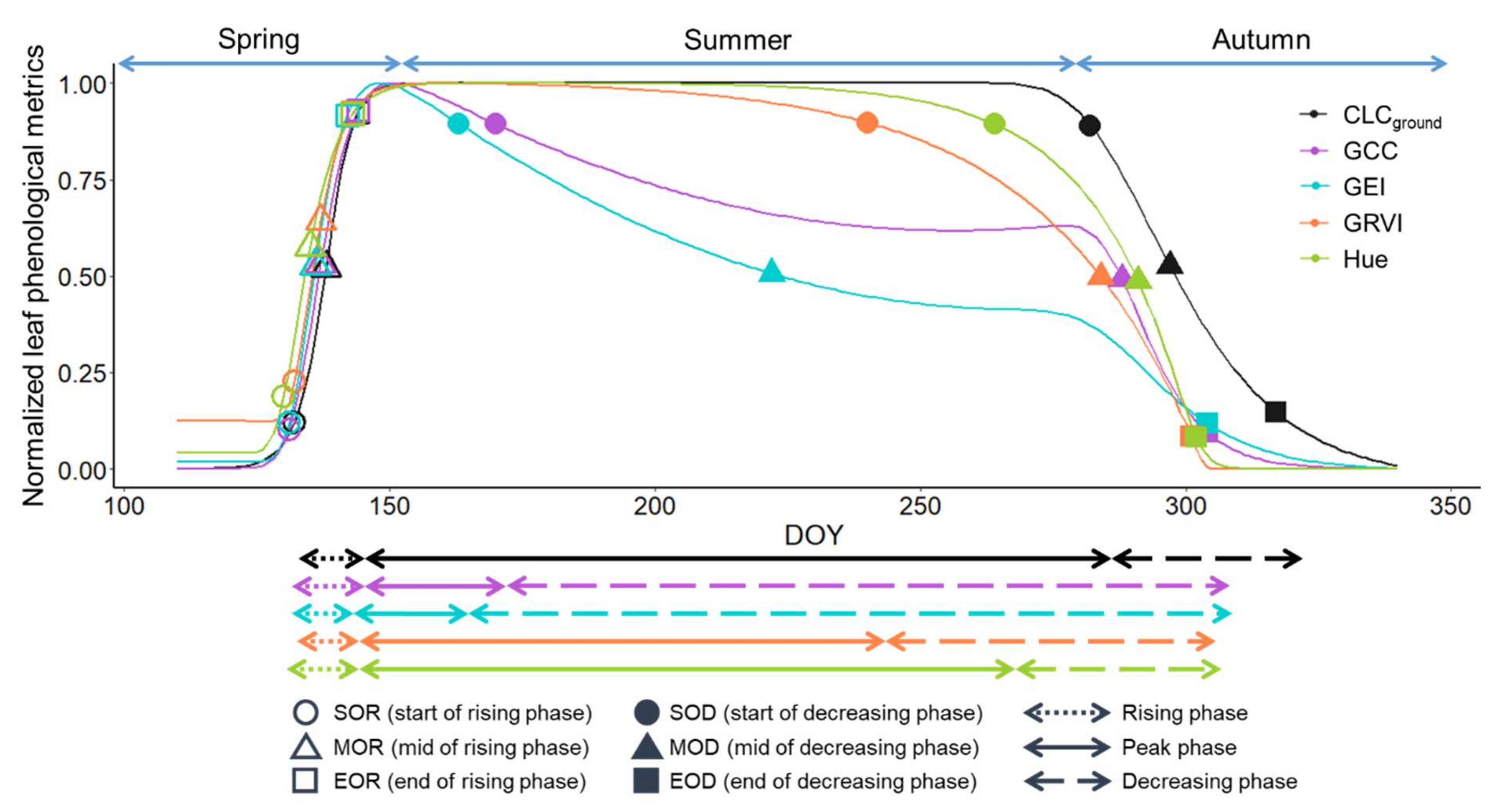
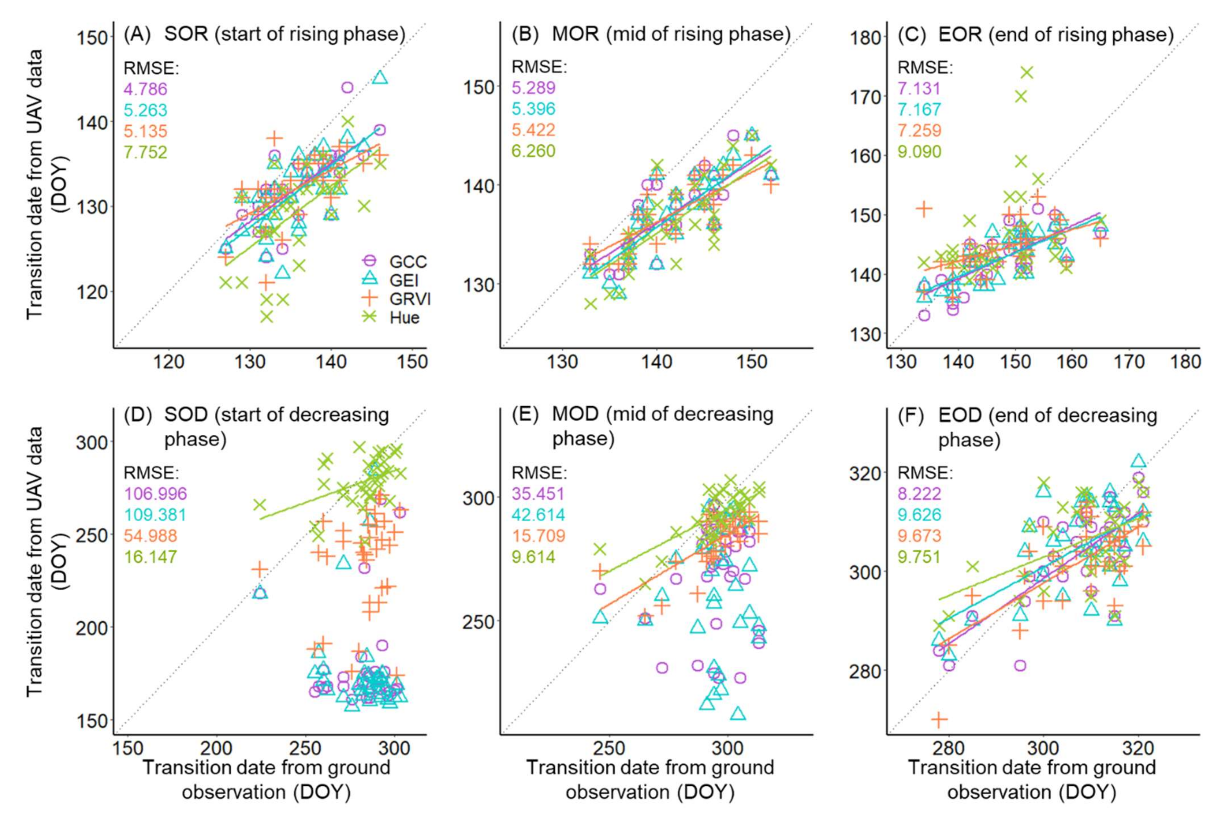
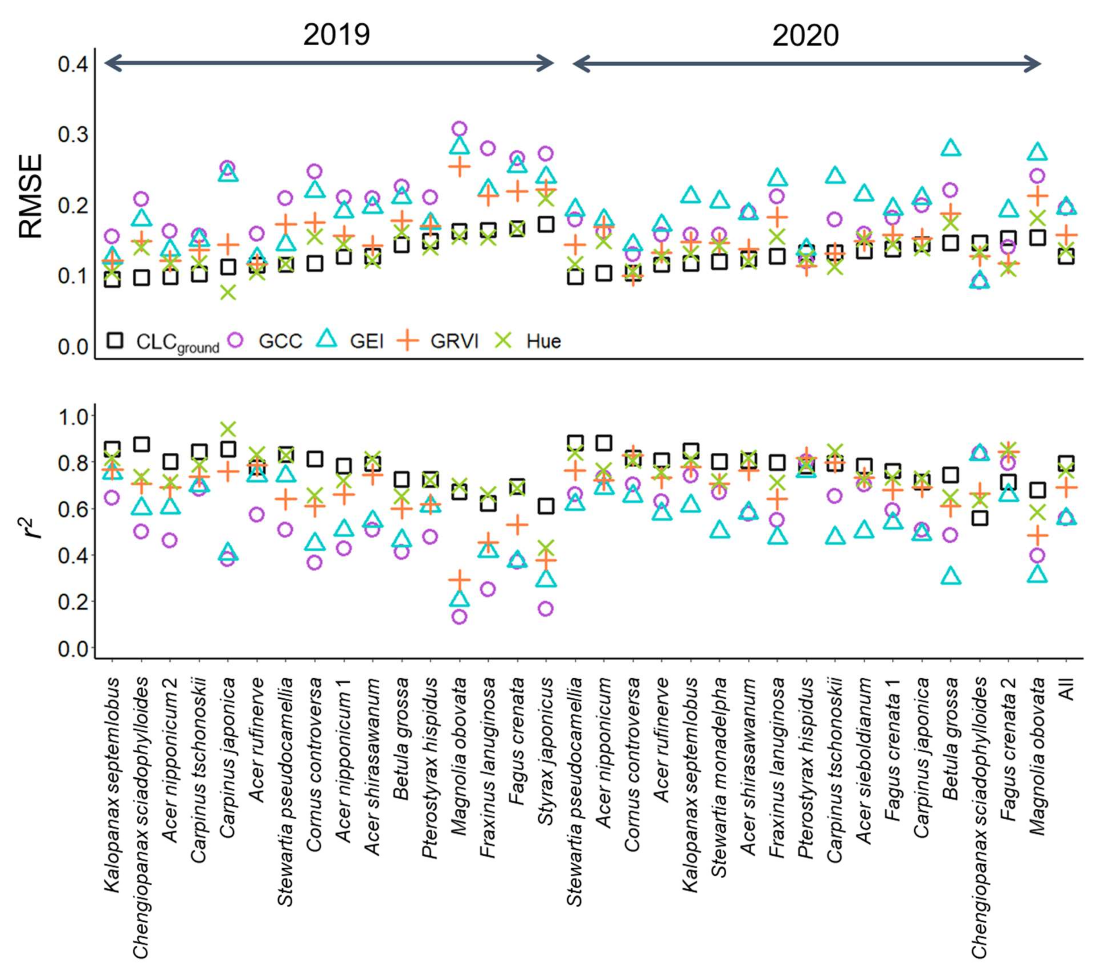
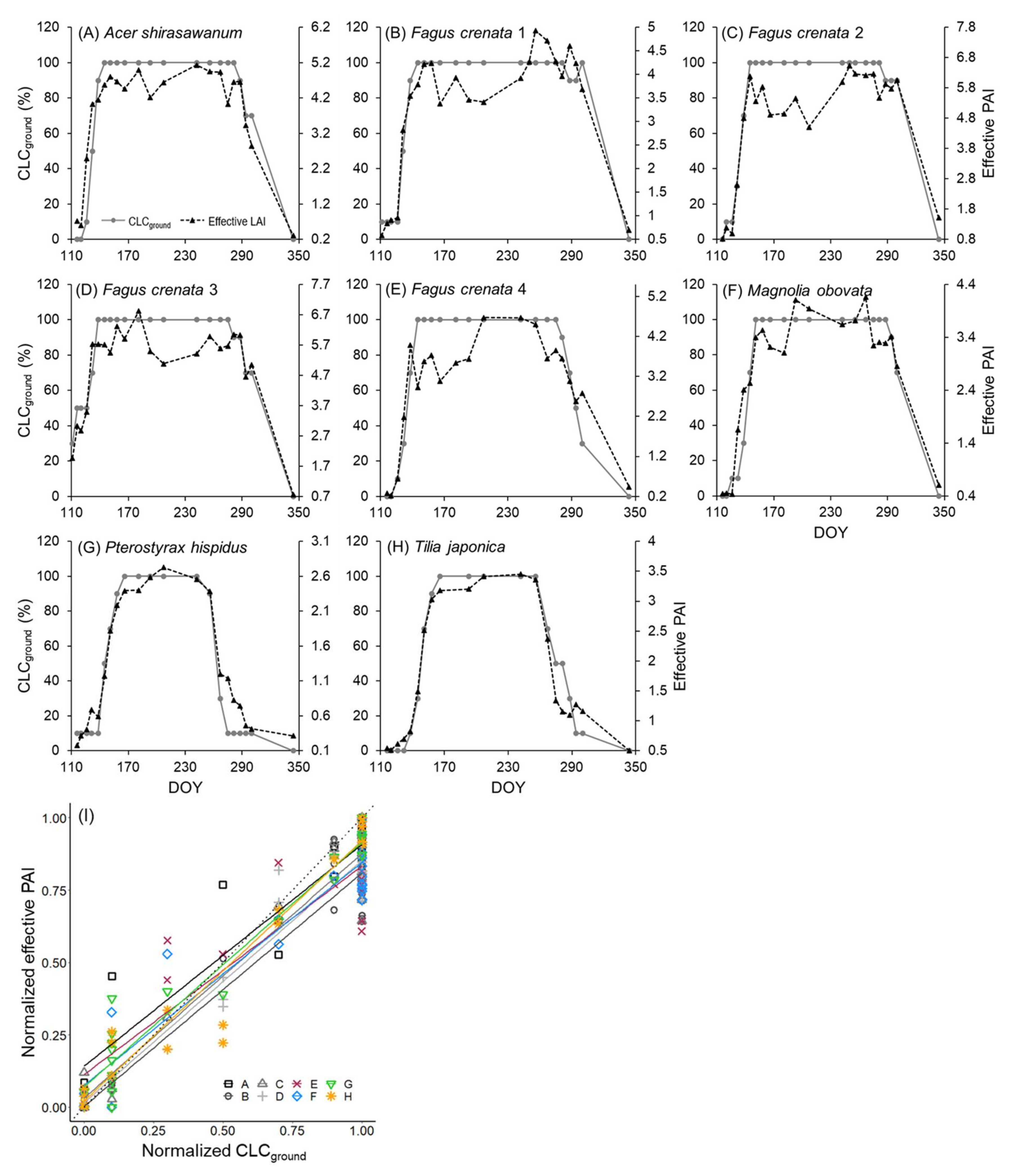
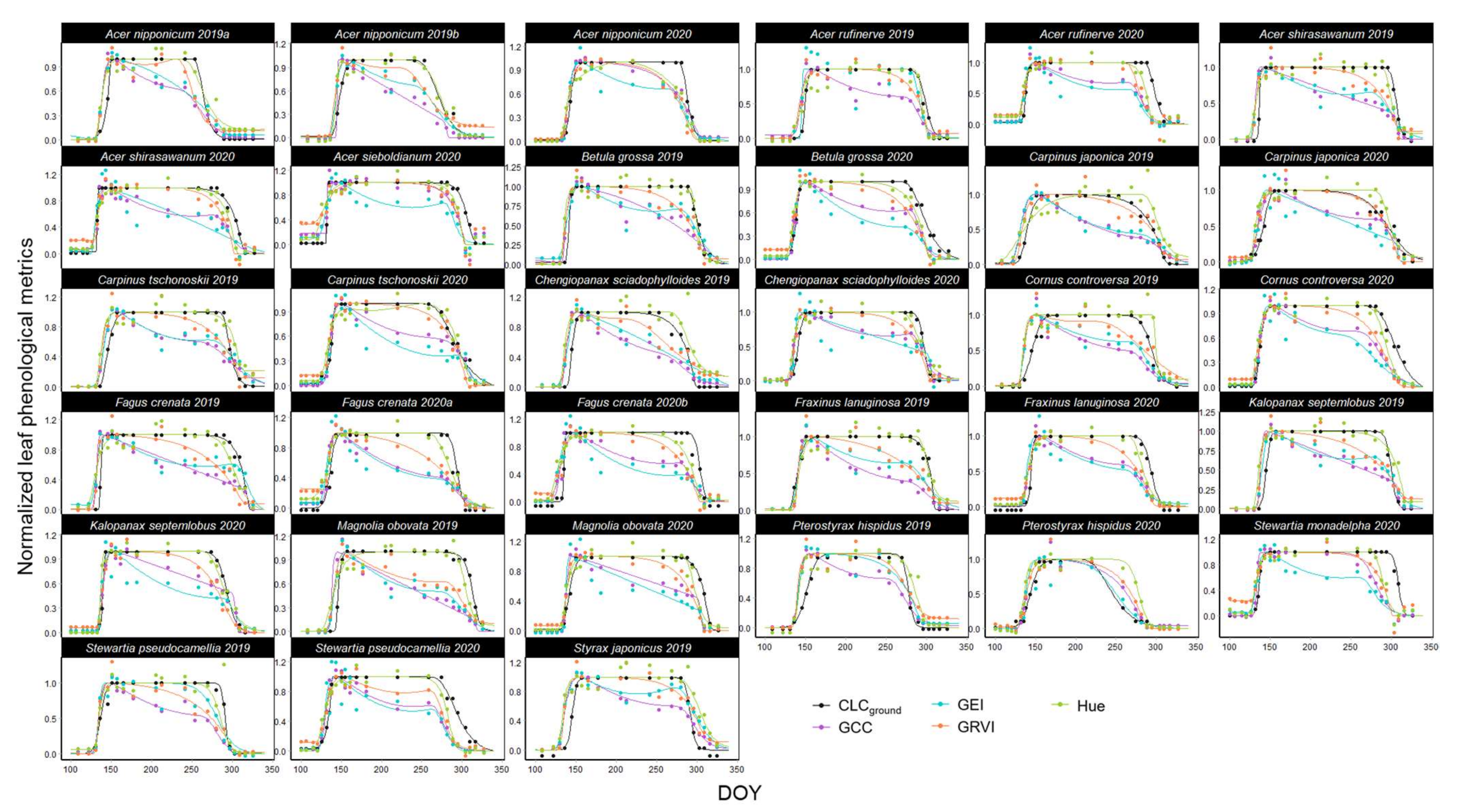
3.1. Leaf Phenology Derived from Ground Observation and UAV Imagery

A typical example of seasonal trajectories of leaf phenological metrics is shown in Figure 1. Although all the metrics showed similar trajectories in the spring, the summer to autumn trajectories were markedly different among the metrics; that is, crown leaf cover based on ground visual observation (CLCground) and Hue had a long peak period, the green chromatic coordinate (GCC), and green excess index (GEI) showed a continuous decline over summer, and the green-red vegetation index (GRVI) had an intermediate pattern between Hue and GCC (Figure 1). These trends were common for all individuals, with several exceptions (e.g., the GEI for Acer rufinerve Siebold & Zucc. in 2019 had a longer peak period than that of the GRVI, Figure A5).
The phenological transition dates derived from CLCground showed large inter-species variations (Figure 2). The mean start and end dates of the spring rising phase (SOR and EOR, respectively) varied by 13.5 and 27 days across the species, respectively. In addition, the mean start and end dates of the decreasing period (SOD and EOD, respectively) varied by 55.5 and 35.5 days, respectively. The climatic conditions in 2020 were characterized by heavier precipitation in July and warmer winter temperature than that in 2019 (Figure A6). Although the influence of such inter-annual variations in climatic conditions was included in the intra-species variations in leaf phenology, the mean intra-species variations in SOR, EOR, SOD, and EOD were 5.4, 6.7, 14.9, and 8.0 days, respectively, which were smaller than the inter-species variations in SOR, EOR, SOD, and EOD.
A comparison of the phenological transition dates derived from CLCground and the UAV metrics is shown in Figure 3. The transition dates derived from the UAV metrics were significantly correlated with those derived from CLCground throughout the spring rising phase irrespective of the type of UAV metric (Figure 3A–C), whereas the RMSE values of the correlations increased as the spring progressed. In contrast, during the decreasing phase, the correlations of the phenological transition dates differed markedly among the UAV metrics, that is, although the Hue-derived transition dates showed significant correlations with the CLCground-derived dates throughout the phase, the GCC and GEI-derived dates were considerably different from the CLCground-derived dates, except for EOD (Figure 3D–F). Regarding GRVI, significant correlations were found in the comparison of MOD and EOD, but not in the comparison of SOD.

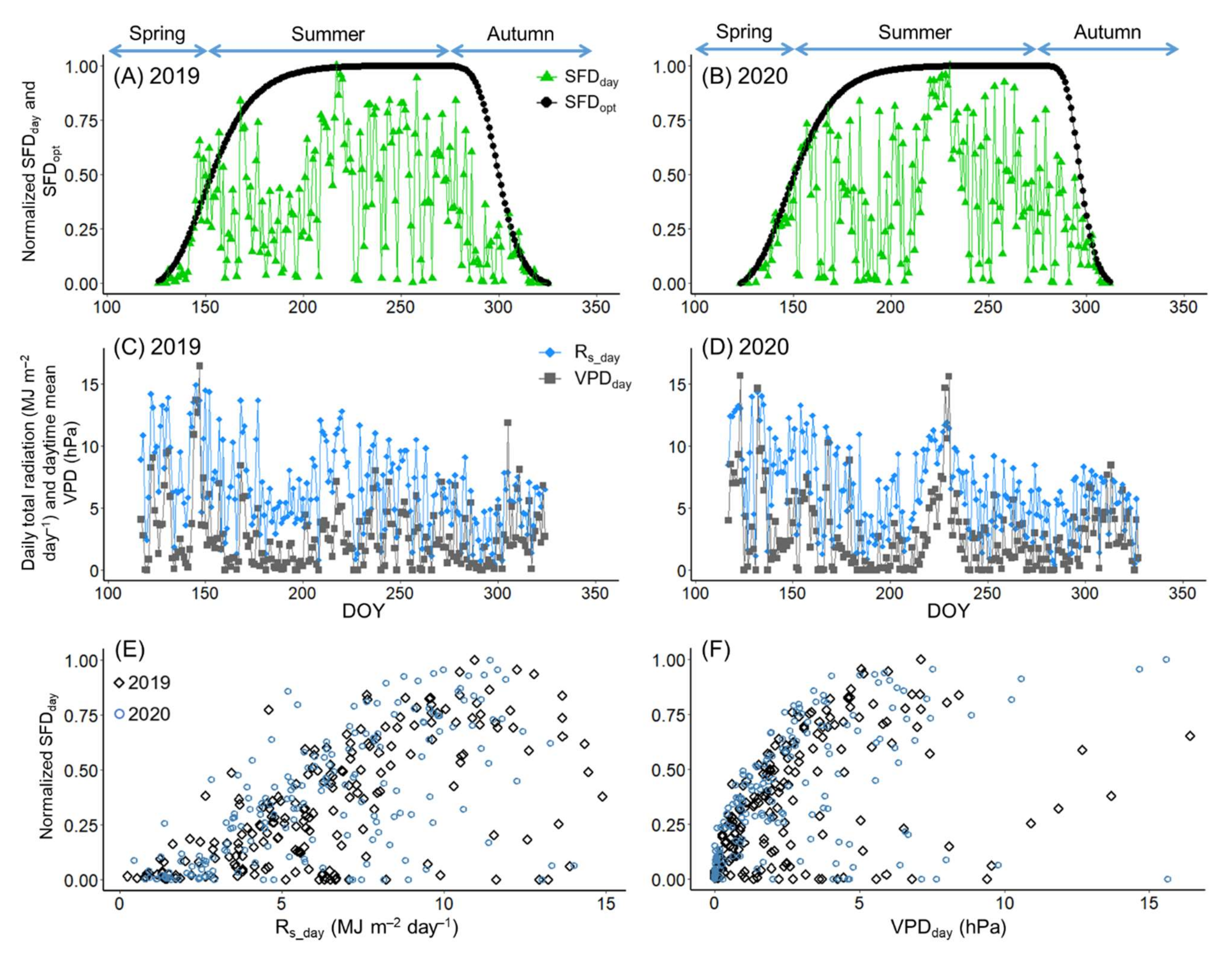
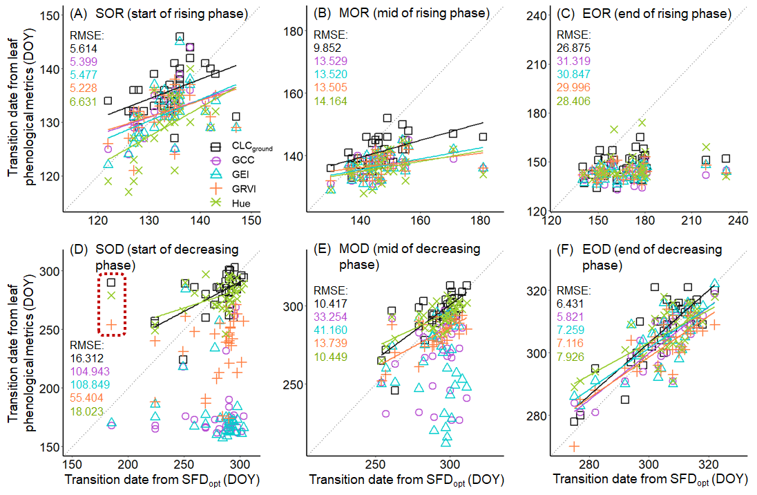
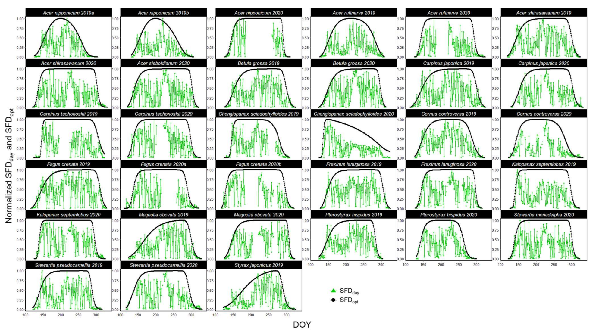
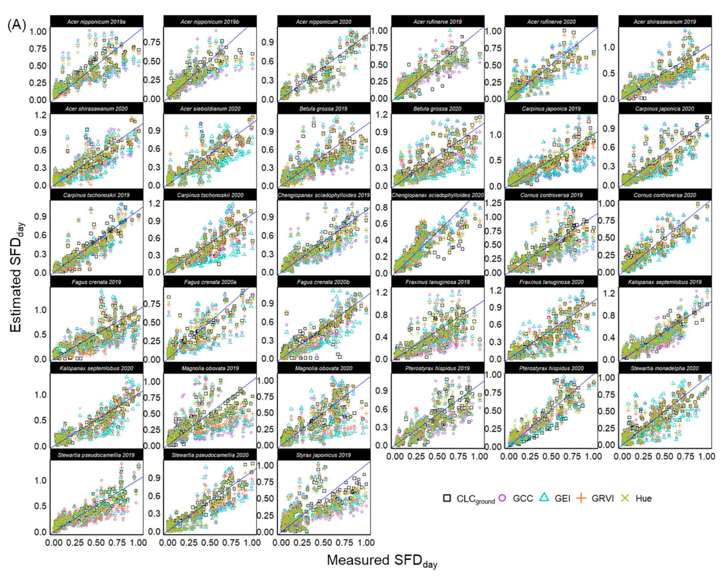
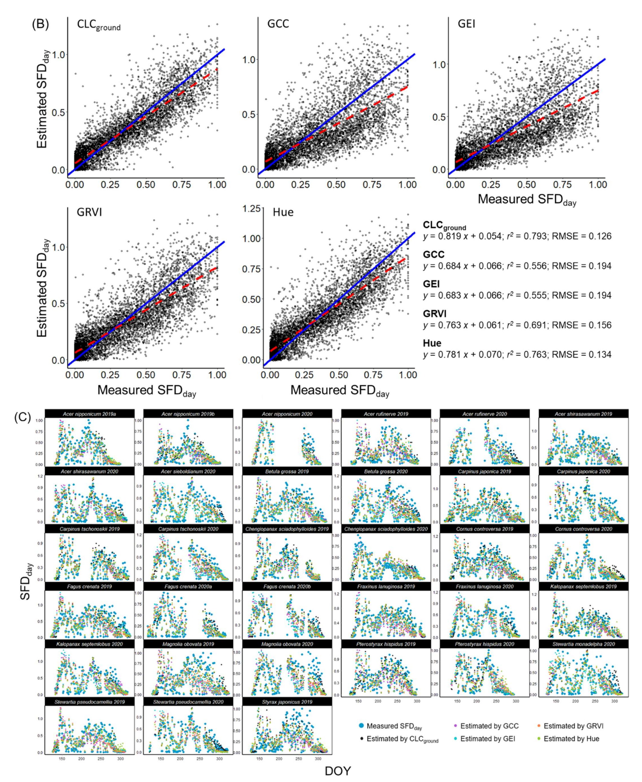
3.2. Sap Flow Phenology and Comparison with Leaf Phenology

The daytime total sap flux density (SFDday) also showed clear seasonality, with high values during summer and low values in early spring and late autumn (Figure 4A,B and Figure A3). However, large day-to-day variations governed by radiation (Rs) and vapor pressure deficit (VPD) were found throughout the seasons, making comparisons between sap flow and leaf phenology difficult (Figure 4C–F). Thus, we estimated SFDday from the phenological metrics using the Bayesian model (Equation (6)), and compared the estimated values with the measured values (Figure 5 and Figure A6). Although significant correlations between the measured and estimated SFDday were found irrespective of the type of phenological metric, predicting ability largely differed among the metrics as follows: CLCground > Hue > GRVI > GCC ≈ GEI. For example, the SFDday estimated by CLCground had the best correlation with the measured data in 20 of the 33 individuals. With respect to Hue, the best correlations were found in 10 of the 33 individuals. In contrast, SFDday estimated by GCC or GEI showed the worst correlations for most individuals, with the exception of the Chengiopanax sciadophylloides (Franch. & Sav.) C.B.Shang & J.Y.Huan tree measured in 2020.
For a more detailed comparison of phenology between leaf and sap flow, we reproduced the optimized SFDday (SFDopt) using Equations (6) and (7) and compared the phenological transition dates of SFDopt and leaf phenological metrics (Figure 6). The SOR derived from the leaf phenological metrics was significantly correlated with that derived from SFDopt irrespective of the type of metric, with an RMSE of less than seven days. However, the RMSE values of the correlations increased as spring progressed, and significant correlations disappeared in comparison with the EOR. In contrast, in the decreasing phase, the RMSE values of the correlations decreased as the seasons progressed. Only the transition dates derived from CLCground and Hue were significantly correlated with those derived from SFDopt throughout the decreasing phase.

4. Discussion

We used two years of concurrent UAV observations and sap flow measurements across 17 species to evaluate the potential of UAV-derived leaf phenological metrics for tracking the seasonal dynamics of sap flow (i.e., sap flow phenology). Although both leaf and sap flow phenology showed large inter- and intra-species variations, daytime total sap flux density (SFDday) estimated by the UAV-derived metrics was significantly correlated with the measured SFDday across species and seasons (Figure 5 and Figure A7), suggesting that UAV-derived metrics have potential as predictors of individual-level sap flow phenology in this ecosystem. However, the predictive ability of the UAV metrics largely differed among the metrics, with Hue showing the highest performance (RMSE = 0.135 for all pooled data), the green chromatic coordinate (GCC) and green excess index (GEI) showing the lowest (RMSE = 0.190), and the green-red vegetation index (GRVI) showing intermediate performance (RMSE = 0.154). The superior performance of Hue has also been reported in ecosystem-level comparisons between photosynthesis and phenocam-derived metrics in temperate deciduous forests [23,24]. Because differences in spring trajectories among the UAV metrics were generally small, the observed differences in predictive ability were attributed to differences in summer to autumn trajectories (Figure 1 and Figure A5), that is, Hue had a long peak period, the GCC and GEI showed a continuous decline, and the GRVI had an intermediate pattern between GCC and Hue.
From summer to autumn, both Hue and CLCground showed similar trajectories with optimized SFDday (SFDopt) for most individuals (Figure 6 and Figure A5), but the overall performance for predicting SFDday was higher for CLCground than for Hue (Figure 5). Because CLCground reflects the phenology of only leaf amount, like leaf area index (LAI), the similar trajectory between CLCground and SFDopt suggests that SFDday during the summer to autumn period is mainly controlled by leaf amount and not by leaf physiological properties, such as stomatal conductance (gs). This might be a surprising result because both leaf amount and leaf gs are important factors for controlling tree transpiration, e.g., [43]; furthermore, previous studies have reported that autumn decreases gs accompanied by leaf coloring, which generally starts before leaf fall in deciduous tree species, e.g., [44,45,46]. On the other hand, empirical evidence indicates that seasonal dynamics of sap flow can be described using environmental factors and LAI in temperate deciduous broad-leaved species [39,47]. Regarding the cause of the small contribution of gs, Hiyama et al. [48] found that gs of colored leaves maintained high values until late autumn in Quercus serrata Murray in a Japanese temperate forest. The stomata of senescent leaves lose responsiveness to environmental variables and cannot be closed efficiently, even under low-light conditions (dull leaf phenomenon [43,49,50]), maintaining leaf gs and thus SFDday at high values during the autumn leaf senescence period. In fact, nighttime SFD tended to increase from summer to autumn for more than half of the sampled trees (Figure A4, [37]), supporting this point of view. Therefore, the lack of stomatal control by leaf senescence may explain why CLCground showed better performance for predicting SFDday than the UAV metrics. This implies that camera-based modelling of SFDday during the summer to autumn period should be based on phenological metrics reflecting changes in leaf amount rather than leaf physiological characteristics for deciduous tree species in cool temperate climates. This finding contrasts with canopy photosynthesis in temperate deciduous forests; that is, autumn decline occurred several weeks earlier for photosynthesis than for LAI, e.g., [9,13], probably because leaf photosynthesis starts to decrease with or before leaf coloring [25]. Although plant transpiration is inevitably linked to photosynthesis through the stomatal control of CO2 absorption, our study suggests that phenological metrics different from photosynthesis should be used to model transpiration phenology.
Although the ability to predict sap flow phenology was slightly lower for Hue than for CLCground, Hue showed a seasonal trajectory similar to that of CLCground compared to the other UAV-derived metrics (Figure 3 and Figure A5). This result is consistent with previous findings that Hue can be used as a proxy for seasonal variations in leaf amount in deciduous broad-leaved species [12,24]. Additionally, Mizunuma et al. [24] showed that Hue values were relatively stable for camera models, camera settings, and sky conditions compared with the other indices. Considering the labor intensity of ground observations, Hue would be a suitable factor for modelling tree transpiration on a large scale. However, the seasonal trajectory of Hue is affected by species-specific differences in leaf color. For example, for species showing bright leaf coloring in autumn, such as Acer sieboldianum Miq., the start date of the decreasing phase (SOD) was 20–30 days earlier for Hue than for CLCground (Figure A5), leading to an underestimation of autumn SFDday. In contrast, for species showing unclear leaf coloring (i.e., with a certain amount of chlorophyll remaining in senescent leaves), such as Pterostyrax hispidus Siebold & Zucc., SOD was markedly later for Hue than CLCground, causing an overestimation of SFDday. The timing and extent of leaf coloring vary not only with species but also with the local growth environments of individual trees and inter-annual variations in climatic conditions [8,51,52]. Therefore, the ability of Hue to predict sap flow phenology can also vary with these factors, which should be considered when Hue is used for modelling transpiration phenology.
Previous research based on tower-mounted phenocams has reported that normalized difference vegetation index (NDVI) is more sensitive to changes in canopy LAI than GCC in deciduous broad-leaved forests [53,54]. This is because NDVI incorporates bands at near-infrared (NIR) wavelengths, where the reflectance of leaves is governed by structural characteristics rather than pigmentation. Therefore, phenological metrics using an NIR band may perform better than Hue. However, because NDVI uses a red color band for the calculation, its seasonal trajectory can also be affected by spatiotemporal variations in leaf color [55,56]. For example, NDVI showed an obvious decrease when leaves turned from green to yellow during early autumn in a Japanese deciduous forest [57]. Although superior characteristics of NDVI compared with metrics calculated from RGB images have been reported at the ecosystem level, no study has compared the seasonality of LAI, NDVI, and Hue at individual tree level. As UAVs equipped with multispectral sensors are commercially available, this issue should be tested in future research.
During spring, although the start date of the rising phase (SOR) derived from the UAV metrics showed good agreement with that derived from SFDopt, the end date (EOR, i.e., spring peak) derived from the UAV metrics preceded that derived from SFDopt by several weeks to two months for more than half of the individuals (Figure 6). Consequently, consistent overestimation of SFDday was found during the rising phase, irrespective of the type of UAV metric (Figure A7). Although studies comparing sap flow and leaf phenology are generally limited, similar discrepancies in the spring peak have been reported in the stand-level comparison for Fagus sylvatica L. [58] and in the branch-level comparison for Rhododendron occidentale (Torr. & A. Gray) A. Gray [59]. Furthermore, large discrepancies in spring peaks have been frequently reported in comparisons between canopy photosynthesis and phenocam-derived phenological metrics at the ecosystem level, e.g., [9,10,13]. For example, Keenan et al. [13] showed that the spring peak of canopy GCC derived from phenocam preceded the peak of gross ecosystem production (GEP) by two weeks in temperate deciduous forests. Since they also found similar discrepancies against canopy LAI and leaf chlorophyll concentration, they concluded that the discrepancy in the spring peak between GEP and GCC could be attributed to the saturation of green signals at low LAI (approximately 2 to 2.5 m2 m−2). However, in this study, not only the UAV-derived metrics but also CLCground, which closely correlated with the effective plant area index derived from hemispherical photography (Figure A2), showed a large discrepancy in the spring peak against SFDopt, implying the involvement of factors other than the saturation of the green signal. Muraoka and Koizumi [25] showed that the annual peak of leaf photosynthetic capacity and gs occurred approximately two months after the peak of leaf chlorophyll concentration and crown leaf area for deciduous broad-leaved tree species in Japanese cool temperate forests. Therefore, late maturation of leaf physiological properties may explain the observed discrepancy in the spring peak between SFDopt and the UAV metrics, as anticipated by Richardson et al. [18].
Because the spatial scale between sap flow and leaf phenological metrics was identical at the tree level in this study, we expected a much closer flux–leaf phenology relationship than the relationships obtained in the ecosystem-level comparison, which involves a mismatch of footprint size between flux and optical measurements [26]. However, contrary to our expectation, a large discrepancy in the spring peak was still observed, indicating that strict matching of footprint size is not always important for evaluating flux–leaf phenology relationships. Instead, disentangling the interaction between leaf physiological properties, crown structure, and reflectance is more important for predicting carbon and water fluxes using a remote sensing approach. Although the spring rising phase is relatively short compared to the peak and decreasing phases during summer and autumn (Figure 1), the transition dates and duration of the rising phase are sensitive to climate change, e.g., [60], which has a significant influence on inter-annual variations in carbon and water flux [5]. To clarify the cause of the systematic discrepancy in spring peak (i.e., EOR) between sap flow and leaf phenology, further data accumulation and combined measurements of leaf phenological metrics and physiological properties, such as gs, chlorophyll fluorescence, and pigment compositions, are necessary.
We are aware of the limitations of our study that should be addressed in future studies. First, the sap flow phenology of individual trees was represented by a single sensor installed at a 0–2 cm depth in the sapwood. Although SFDday generally decreases with increasing sapwood depth, previous studies have shown that ignoring radial variations in SFDday causes considerable errors in estimates of tree transpiration, e.g., [38]. Furthermore, the radial profile of SFDday can vary during the season and is correlated with changes in environmental conditions, such as air VPD [61], soil-water content [37,62,63], and irradiance [64]. If such seasonality was present in the radial profile of the SFDday of our investigated species, the SFD obtained from single-sensor measurements would not reproduce sap flow phenology correctly. Therefore, future studies should investigate spatiotemporal variations in SFD within stems to reproduce sap flow phenology at the tree level. Second, reductions in SFDday due to drought stress are rare at this site because of frequent rain events. However, since inter-annual variations in precipitation have tended to increase in Japan since the 1970s (Japan Meteorological Agency), drought conditions may be created in future rainless years. Previous studies have demonstrated that camera-derived leaf phenological metrics cannot detect drought-dependent decreases in physiological properties when canopy color does not change with drought, e.g., [9]. Therefore, two years of observation may be too short to characterize flux–leaf phenology relationships. To enhance the generic applicability of our study results, further data accumulation through long-term monitoring is necessary. Third, image acquisitions using the UAV were often conducted in variable illumination conditions because of rapidly changing regional weather (i.e., frequent fog and cloud cover, Table A1), which causes large spatiotemporal variations in brightness on the canopy surface, creating a bias in phenological metric estimation at the individual tree level. Although the seasonal amplitude of the phenological metrics is markedly greater than that of noise induced by variable illumination conditions in deciduous trees [27,65], homogeneous illumination conditions are still considered essential for precise estimation of phenological metrics. In unstable weather conditions, such as those in the study site, flight time should be shortened by increasing flight height and adopting higher resolution cameras.

5. Conclusions

Although we chose various species with different successional strategies and crown structures, Hue showed close correlations with sap flow phenology across the species because sap flow phenology, especially during summer to autumn, is explained by changes in leaf amount (i.e., CLCground) for most of the individuals, and the Hue is closely correlated with CLCground. Therefore, UAV observations have the potential to track tree-level sap flow phenology for deciduous broad-leaved species in cool temperate climate forests, which can contribute to the accurate prediction of transpiration in forests with complex vegetation structures. However, during the spring rising period, UAV-derived phenological metrics showed a more pronounced early peak than sap flow phenology, irrespective of the type of metric, probably due to earlier development of leaf area than leaf physiological properties. For a more accurate prediction of sap flow phenology, exploration of reflectance indices for tracking spring sap flow should be conducted in future studies.

Author Contributions

Conceptualization, A.I.; methodology, A.I. and N.B.; validation, N.B., A.I. and M.N.; formal analysis, N.B. and A.I.; investigation, N.B.; resources, A.I.; data curation, N.B.; writing—original draft preparation, N.B.; writing—review and editing, A.I. and M.N.; visualization, N.B.; supervision, A.I. and M.N.; project administration, A.I.; funding acquisition, A.I. All authors have read and agreed to the published version of the manuscript.

Funding

This research was funded by KAKENHI, grant number 18H02236 (Grant-in-Aid for Scientific Research B by the Japan Society for the Promotion of Science).

Data Availability Statement

The data presented in this study are available on request from the corresponding author.

Acknowledgments

The authors thank Hiromi Mizunaga of Shizuoka University and Hiroyuki Muraoka of Gifu University for their critical comments, and the students of the Silviculture Laboratory of Shizuoka University who assisted with field research. N. Budianti was supported by the English special program of the Gifu University.

Conflicts of Interest

The authors declare no conflict of interest.

Abbreviations

CLCgroundCrown leaf cover derived from ground observation
EODEnd of the decreasing phase
EOREnd of the rising phase
GEIGreen excess index
GRVIGreen-red vegetation index
gsStomatal conductance
LAILeaf area index
MODMid of the decreasing phase
MORMid of the rising phase
RMSERoot-mean-square error
RsSolar radiation
SFDSap flux density
SFDdayDaytime (05:00–20:00) total sap flux density
SFDoptOptimized daytime sap flux density
SODStart of the decreasing phase
SORStart of the rising phase
UAVUnmanned aerial vehicle
VPDVapor pressure deficit

Appendix A

Figure A1. Orthophoto of the study site acquired on 25 May 2019 (DOY 145) showing location of ground control points, towers, and field accommodation and the area of sap flow measurement.
Remotesensing 14 02505 g0a1
Figure A2. Comparison between effective plant area index (PAI) derived from digital hemispherical photographs (DHP) and crown leaf cover based on the ground observation (CLCground) for eight canopy trees measured in 2021. To quantify effective PAI from DHP at individual tree level, we chose samples with a large crown but small influence from neighboring trees. The DHP images were acquired using a Nikon D5100 camera (Nikon, Tokyo, Japan) fitted with a 4.5-mm F2.8 EX DC circular fisheye converter (SIGMA, Kanagawa, Japan) and were imported into ImageJ software for post-processing. We defined the processing range for DHP using the circle of interest adjusted according to the crown edges of the individual trees, and calculated effective PAI using CIMES software [66]. All values on panel (I) are normalized to a scale of 0 to 1. Dotted lines are 1:1 lines, and solid lines are linear regression equations as follows: (A) y = 0.766x + 0.142, r2 = 0.886, root mean square error (RMSE) = 0.140; (B) y = 0.806x + 0.003, r2 = 0.903, RMSE = 0.191; (C) y = 0.844x + 0.032, r2 = 0.912, RMSE = 0.144; (D) y = 0.838x + 0.015, r2 = 0.876, RMSE = 0.152; (E) y = 0.720x + 0.113, r2 = 0.828, RMSE = 0.187; (F) y = 0.769x + 0.076, r2 = 0.902, RMSE = 0.164; (G) y = 0.845x + 0.070, r2 = 0.945, RMSE = 0.104; (H) y = 0.899x + 0.022, r2 = 0.943, RMSE = 0.101.
Remotesensing 14 02505 g0a2
Figure A3. Seasonal trajectories of daytime total sap flux density (SFDday) and the optimized SFD (SFDopt) derived from Equations (6) and (7) for all individuals. All values are normalized to the scale from 0 and 1. Abbreviation: DOY, day of the year.
Remotesensing 14 02505 g0a3
Figure A4. Seasonal dynamics of daytime and nighttime sap flux density (SFD) for four representative trees measured in 2019. Nighttime SFD gradually increased from spring to autumn and was found in 19 of the 33 individuals. Abbreviation: DOY, day of the year.
Remotesensing 14 02505 g0a4
Figure A5. Time series of the leaf phenological metrics for all individual trees. Solid lines are fitted results of double logistic models. Fitted results are normalized to a scale from 0 to 1, and the scale of the phenological metrics was adjusted accordingly. Abbreviations: CLCground, crown leaf cover based on the ground observation; GCC, green chromatic coordinate; GEI, green excess index; GRVI, green-red vegetation index; DOY, day of the year.
Remotesensing 14 02505 g0a5
Figure A6. Monthly mean air temperature (T) and solar radiation (Rs), and monthly total precipitation in 2019 and 2020. Precipitation data were taken from the data of the Kawanehoncho meteorological station (the Japan Meteorological Agency, 2021). Error bars indicate the standard deviation.
Remotesensing 14 02505 g0a6
Figure A7. Comparison of the daytime total sap flux density (SFDday) values estimated by leaf phenological metrics and the measured values; individual trees basis (A), all pooled data (B), and comparison of seasonal trajectories (C). Measured SFDday values are normalized to the scale from 0 to 1, and the scale of the estimated SFDday was adjusted accordingly. The solid lines in panels (A,B) are 1:1 lines. Root-mean-square error and coefficient of determination of linear regression analysis for the data in panels (A,B) are shown in Figure 5. Abbreviations: CLCground, crown leaf cover based on the ground observation; GCC, green chromatic coordinate; GEI, green excess index; GRVI, green-red vegetation index; DOY, day of the year.
Remotesensing 14 02505 g0a7aRemotesensing 14 02505 g0a7b
Table A1. Details of the UAV survey and quality of the orthophoto derived using Context Capture. Abbreviations: DOY, day of the year; RMSE, root-mean-square error; nd, not determined. * Two of the seven ground control points (GCPs) showed high RMSE values (1.7–2.0 m) due to a small number of overlapping aerial photos around the GCPs.
YearDateDOYFlight TimeMean ± SD Radiation during the Flight
(J m−2 s−1)
Number of Photos Used for Orthophoto ProductionAverage Ground Resolution
(cm Pixel−1)
RMSE of Reprojection
(Pixel)
3D RSME of GCPs
(m)
201918 April10810:30–12:19N/A30121.620.620.003
02 May12209:44–10:51466.8 ± 38.712641.470.580.021
10 May13010:09–12:28453.1 ± 14.230991.550.690.000
16 May13611:05–12:28262.7 ± 26.430921.150.840.001
25 May14511:05–13:24505.0 ± 18.512081.170.720.001
31 May15110:02–12:22222.2 ± 80.611780.910.710.001
06 May15710:24–11:29532.5 ± 103.717031.300.800.001
14 June16509:25–11:19191.9 ± 67.630081.400.810.001
26 June17710:00–11:44440.9 ± 37.616931.000.850.048
24 July20512:15–12:35398.3 ± 85.67691.270.740.001
31 July21211:08–11:47379.6 ± 151.35361.260.720.000
29 August24115:03–16:23108.2 ± 8.420681.110.800.052
10 September25311:26–13:17388.8 ± 47.421821.200.670.055
26 September26912:10–13:44249.2 ± 78.018501.290.740.048
07 October28010:59–12:31275.3 ± 42.324101.100.720.074
16 October28914:39–15:3196.4 ± 45.412661.010.700.044
23 October29610:36–11:50220.3 ± 29.014121.020.670.060
30 October30310:30–11:48336.5 ± 13.410421.040.600.023
05 November30910:37–12:08305.7 ± 36.8ndndndnd
12 November31610:15–11:33298.44 ± 18.0ndndndnd
21 November32510:39–12:27N/Andndndnd
202009 April10012:06–13:57438.9 ± 28.324751.370.620.054
15 April10610:07–12:00434.6 ± 41.025061.460.600.040
24 April11509:25–11:45439.4 ± 49.122711.240.621.172 *
29 April12010:32–12:18469.3 ± 13.723181.190.610.966 *
05 May12610:17–12:17315.8 ± 119.722801.230.600.027
11 May13210:04–11:40477.9 ± 43.721581.270.710.096
14 May13510:10–12:35480.8 ± 19.026141.140.770.089
17 May13810:19–11:46460.9 ± 68.825711.050.710.096
22 May14310:25–12:17292.7 ± 73.724931.120.770.050
29 May15009:59–11:58394.3 ± 111.923051.050.700.106
03 June15509:49–11:25372.4 ± 41.733670.980.670.049
09 June16110:04–11:41348.7 ± 76.723100.880.690.090
17 June16913:24–14:33183.7 ± 61.715341.030.790.054
29 June18109:55–11:16299.1 ± 94.918730.890.740.062
07 August22010:24–12:06392.9 ± 33.118861.060.800.060
14 September25810:20–12:31341.7 ± 52.822180.940.660.102
30 September27408:18–10:24280.9 ± 66.723221.360.600.047
07 October28110:15–11:35262.9 ± 47.120360.990.690.062
14 October28809:16–10:58183.3 ± 32.719200.910.600.053
20 October29411:10–12:58353.9 ± 10.425850.980.630.063
30 October30409:16–10:58199.7 ± 119.624070.890.600.116
04 November30914:17–14:58213.8 ± 40.210741.150.610.055
11 November31610:05–11:05305.3 ± 29.914451.360.570.246
22 November32710:43–11:5582.0 ± 16.614301.250.580.042

References

  1. Vitasse, Y.; Porté, A.J.; Kremer, A.; Michalet, R.; Delzon, S. Responses of canopy duration to temperature changes in four temperate tree species: Relative contributions of spring and autumn leaf phenology. Oecologia 2009, 161, 187–198. [Google Scholar] [CrossRef] [PubMed]
  2. Zhang, H.; Yuan, W.; Liu, S.; Dong, W. Divergent responses of leaf phenology to changing temperature among plant species and geographical regions. Ecosphere 2015, 6, art250. [Google Scholar] [CrossRef]
  3. Shen, M.; Tang, Y.; Chen, J.; Yang, X.; Wang, C.; Cui, X.; Yang, Y.; Han, L.; Li, L.; Du, J.; et al. Earlier-Season Vegetation Has Greater Temperature Sensitivity of Spring Phenology in Northern Hemisphere. PLoS ONE 2014, 9, e88178. [Google Scholar] [CrossRef] [PubMed]
  4. Gill, A.L.; Gallinat, A.S.; Sanders-DeMott, R.; Rigden, A.J.; Short Gianotti, D.J.; Mantooth, J.A.; Templer, P.H. Changes in autumn senescence in northern hemisphere deciduous trees: A meta-analysis of autumn phenology studies. Ann. Bot. 2015, 116, 875–888. [Google Scholar] [CrossRef] [PubMed] [Green Version]
  5. Richardson, A.D.; Keenan, T.F.; Migliavacca, M.; Ryu, Y.; Sonnentag, O.; Toomey, M. Climate change, phenology, and phenological control of vegetation feedbacks to the climate system. Agric. For. Meteorol. 2013, 169, 156–173. [Google Scholar] [CrossRef]
  6. Vitasse, Y.; Basler, D. What role for photoperiod in the bud burst phenology of European beech. Eur. J. For. Res. 2013, 132, 1–8. [Google Scholar] [CrossRef]
  7. Fu, Y.S.H.; Campioli, M.; Vitasse, Y.; De Boeck, H.J.; Van Den Berge, J.; AbdElgawad, H.; Asard, H.; Piao, S.; Deckmyn, G.; Janssens, I.A. Variation in leaf flushing date influences autumnal senescence and next year’s flushing date in two temperate tree species. Proc. Natl. Acad. Sci. USA 2014, 111, 7355–7360. [Google Scholar] [CrossRef] [Green Version]
  8. Xie, Y.; Wang, X.; Wilson, A.M.; Silander, J.A. Predicting autumn phenology: How deciduous tree species respond to weather stressors. Agric. For. Meteorol. 2018, 250–251, 127–137. [Google Scholar] [CrossRef]
  9. Toomey, M.; Friedl, M.A.; Frolking, S.; Hufkens, K.; Klosterman, S.; Sonnentag, O.; Baldocchi, D.D.; Bernacchi, C.J.; Biraud, S.C.; Bohrer, G.; et al. Greenness indices from digital cameras predict the timing and seasonal dynamics of canopy-scale photosynthesis. Ecol. Appl. 2015, 25, 99–115. [Google Scholar] [CrossRef] [Green Version]
  10. Ahrends, H.E.; Etzold, S.; Kutsch, W.L.; Stoeckli, R.; Bruegger, R.; Jeanneret, F.; Wanner, H.; Buchmann, N.; Eugster, W. Tree phenology and carbon dioxide fluxes: Use of digital photography for process-based interpretation at the ecosystem scale. Clim. Res. 2009, 39, 261–274. [Google Scholar] [CrossRef] [Green Version]
  11. Richardson, A.D.; Braswell, B.H.; Hollinger, D.Y.; Jenkins, J.P.; Ollinger, S.V. Near-surface remote sensing of spatial and temporal variation in canopy phenology. Ecol. Appl. 2009, 19, 1417–1428. [Google Scholar] [CrossRef]
  12. Nagai, S.; Maeda, T.; Gamo, M.; Muraoka, H.; Suzuki, R.; Nasahara, K.N. Using digital camera images to detect canopy condition of deciduous broad-leaved trees. Plant Ecol. Divers. 2011, 4, 79–89. [Google Scholar] [CrossRef]
  13. Keenan, T.F.; Darby, B.; Felts, E.; Sonnentag, O.; Friedl, M.A.; Hufkens, K.; O’Keefe, J.; Klosterman, S.; Munger, J.W.; Toomey, M.; et al. Tracking forest phenology and seasonal physiology using digital repeat photography: A critical assessment. Ecol. Appl. 2014, 24, 1478–1489. [Google Scholar] [CrossRef] [PubMed] [Green Version]
  14. Wingate, L.; Ogeé, J.; Cremonese, E.; Filippa, G.; Mizunuma, T.; Migliavacca, M.; Moisy, C.; Wilkinson, M.; Moureaux, C.; Wohlfahrt, G.; et al. Interpreting canopy development and physiology using a European phenology camera network at flux sites. Biogeosciences 2015, 12, 5995–6015. [Google Scholar] [CrossRef] [Green Version]
  15. Liu, Z.; Hu, H.; Yu, H.; Yang, X.; Yang, H.; Ruan, C.; Wang, Y.; Tang, J. Relationship between leaf physiologic traits and canopy color indices during the leaf expansion period in an oak forest. Ecosphere 2015, 6, 1–9. [Google Scholar] [CrossRef]
  16. Liu, Z.; An, S.; Lu, X.; Hu, H.; Tang, J. Using canopy greenness index to identify leaf ecophysiological traits during the foliar senescence in an oak forest. Ecosphere 2018, 9, 1–14. [Google Scholar] [CrossRef]
  17. Toda, M.; Richardson, A.D. Estimation of plant area index and phenological transition dates from digital repeat photography and radiometric approaches in a hardwood forest in the Northeastern United States. Agric. For. Meteorol. 2018, 249, 457–466. [Google Scholar] [CrossRef]
  18. Richardson, A.D.; Jenkins, J.P.; Braswell, B.H.; Hollinger, D.Y.; Ollinger, S.V.; Smith, M.L. Use of digital webcam images to track spring green-up in a deciduous broadleaf forest. Oecologia 2007, 152, 323–334. [Google Scholar] [CrossRef]
  19. Richardson, A.D.; Hollinger, D.Y.; Dail, D.B.; Lee, J.T.; Munger, J.W.; O’Keefe, J. Influence of spring phenology on seasonal and annual carbon balance in two contrasting New England forests. Tree Physiol. 2009, 29, 321–331. [Google Scholar] [CrossRef]
  20. Moore, C.E.; Brown, T.; Keenan, T.F.; Duursma, R.A.; van Dijk, A.I.J.M.; Beringer, J.; Culvenor, D.; Evans, B.; Huete, A.; Hutley, L.B.; et al. Reviews and syntheses: Australian vegetation phenology: New insights from satellite remote sensing and digital repeat photography. Biogeosciences 2016, 13, 5085–5102. [Google Scholar] [CrossRef] [Green Version]
  21. Zhou, L.; He, H.L.; Sun, X.M.; Zhang, L.; Yu, G.R.; Ren, X.L.; Wang, J.Y.; Zhao, F.H. Modeling winter wheat phenology and carbon dioxide fluxes at the ecosystem scale based on digital photography and eddy covariance data. Ecol. Inform. 2013, 18, 69–78. [Google Scholar] [CrossRef]
  22. Ide, R.; Nakaji, T.; Motohka, T.; Oguma, H. Advantages of visible-band spectral remote sensing at both satellite and near-surface scales for monitoring the seasonal dynamics of GPP in a Japanese larch forest. J. Agric. Meteorol. 2011, 67, 75–84. [Google Scholar] [CrossRef] [Green Version]
  23. Saitoh, T.M.; Nagai, S.; Saigusa, N.; Kobayashi, H.; Suzuki, R.; Nasahara, K.N.; Muraoka, H. Assessing the use of camera-based indices for characterizing canopy phenology in relation to gross primary production in a deciduous broad-leaved and an evergreen coniferous forest in Japan. Ecol. Inform. 2012, 11, 45–54. [Google Scholar] [CrossRef]
  24. Mizunuma, T.; Wilkinson, M.; Eaton, E.L.; Mencuccini, M.; Morison, J.I.L.; Grace, J. The relationship between carbon dioxide uptake and canopy colour from two camera systems in a deciduous forest in southern England. Funct. Ecol. 2013, 27, 196–207. [Google Scholar] [CrossRef]
  25. Muraoka, H.; Koizumi, H. Photosynthetic and structural characteristics of canopy and shrub trees in a cool-temperate deciduous broadleaved forest: Implication to the ecosystem carbon gain. Agric. For. Meteorol. 2005, 134, 39–59. [Google Scholar] [CrossRef]
  26. Yang, J.C.; Magney, T.S.; Yan, D.; Knowles, J.F.; Smith, W.K.; Scott, R.L.; Barron-Gafford, G.A. The photochemical reflectance index (PRI) captures the ecohydrologic sensitivity of a semiarid mixed conifer forest. J. Geophys. Res. Biogeosci. 2020, 125, e2019JG005624. [Google Scholar] [CrossRef]
  27. Klosterman, S.; Richardson, A.D. Observing spring and fall phenology in a deciduous forest with aerial drone imagery. Sensors 2017, 17, 2852. [Google Scholar] [CrossRef] [Green Version]
  28. Budianti, N.; Mizunaga, H.; Iio, A. Crown structure explains the discrepancy in leaf phenology metrics derived from ground- and UAV-based observations in a Japanese cool temperate deciduous forest. Forests 2021, 12, 425. [Google Scholar] [CrossRef]
  29. Medhurst, J.; Parsby, J.; Linder, S.; Wallin, G.; Ceschia, E.; Slaney, M. A whole-tree chamber system for examining tree-level physiological responses of field-grown trees to environmental variation and climate change. Plant Cell Environ. 2006, 29, 1853–1869. [Google Scholar] [CrossRef] [Green Version]
  30. Michelot, A.; Eglin, T.; Dufrene, E.; Lelarge-Trouverie, C.; Damesin, C. Comparison of seasonal variations in water-use efficiency calculated from the carbon isotope composition of tree rings and flux data in a temperate forest. Plant. Cell Environ. 2011, 34, 230–244. [Google Scholar] [CrossRef]
  31. Du, B.; Zheng, J.; Ji, H.; Zhu, Y.; Yuan, J.; Wen, J.; Kang, H.; Liu, C. Stable carbon isotope used to estimate water use efficiency can effectively indicate seasonal variation in leaf stoichiometry. Ecol. Indic. 2021, 121, 107250. [Google Scholar] [CrossRef]
  32. Niinemets, Ü.; Valladares, F. Tolerance to shade, drought, and waterlogging of temperate northern hemisphere trees and shrubs. Ecol. Monogr. 2006, 76, 521–547. [Google Scholar] [CrossRef]
  33. Bentley ContextCapture User Guide. Available online: https://docs.bentley.com/LiveContent/web/ContextCapture_User_Guide_EN_PDF-v18/en/ContextCapture User Guide EN.pdf (accessed on 13 April 2022).
  34. Granier, A. Evaluation of transpiration in a Douglas-fir stand by means of sap flow measurements. Tree Physiol. 1987, 3, 309–320. [Google Scholar] [CrossRef] [PubMed]
  35. Tetens, O. Uber einige meteorologische Begriffe. Z. Geophys. 1930, 6, 297–309. [Google Scholar]
  36. Steppe, K.; De Pauw, D.J.W.; Doody, T.M.; Teskey, R.O. A comparison of sap flux density using thermal dissipation, heat pulse velocity and heat field deformation methods. Agric. For. Meteorol. 2010, 150, 1046–1056. [Google Scholar] [CrossRef]
  37. Ford, C.R.; McGuire, M.A.; Mitchell, R.J.; Teskey, R.O. Assessing variation in the radial profile of sap flux density in Pinus species and its effect on daily water use. Tree Physiol. 2004, 24, 241–249. [Google Scholar] [CrossRef] [Green Version]
  38. Shinohara, Y.; Tsuruta, K.; Ogura, A.; Noto, F.; Komatsu, H.; Otsuki, K.; Maruyama, T. Azimuthal and radial variations in sap flux density and effects on stand-scale transpiration estimates in a Japanese cedar forest. Tree Physiol. 2013, 33, 550–558. [Google Scholar] [CrossRef] [Green Version]
  39. Wullschleger, S.D.; Hanson, P.J.; Todd, D.E. Transpiration from a multi-species deciduous forest as estimated by xylem sap flow techniques. For. Ecol. Manag. 2001, 143, 205–213. [Google Scholar] [CrossRef]
  40. Gu, L.; Post, W.M.; Baldocchi, D.D.; Black, T.A.; Suyker, A.E.; Verma, S.B.; Vesala, T.; Wofsy, S.C. Characterizing the seasonal dynamics of plant community photosynthesis across a range of vegetation types. In Phenology of Ecosystem Processes: Applications in Global Change Research; Noormets, A., Ed.; Springer: New York, NY, USA, 2009; pp. 35–58. ISBN 978-1-4419-0026-5. [Google Scholar]
  41. Quo, J.; Gabry, J.; Goodrich, B.; Weber, S. RStan: The R interface to Stan, Version 2.21.2. 2020. Available online: https://mc-stan.org/rstan (accessed on 9 November 2020).
  42. Filippa, G.; Cremonese, E.; Migliavacca, M.; Galvagno, M.; Forkel, M.; Wingate, L.; Tomelleri, E.; Morra di Cella, U.; Richardson, A.D. Phenopix: A R package for image-based vegetation phenology. Agric. For. Meteorol. 2016, 220, 141–150. [Google Scholar] [CrossRef] [Green Version]
  43. Barnard, D.M.; Bauerle, W.L. The implications of minimum stomatal conductance on modeling water flux in forest canopies. J. Geophys. Res. Biogeosci. 2013, 118, 1322–1333. [Google Scholar] [CrossRef]
  44. Matsumoto, K.; Ohta, T.; Tanaka, T. Dependence of stomatal conductance on leaf chlorophyll concentration and meteorological variables. Agric. For. Meteorol. 2005, 132, 44–57. [Google Scholar] [CrossRef]
  45. Croft, H.; Chen, J.M.; Luo, X.; Bartlett, P.; Chen, B.; Staebler, R.M. Leaf chlorophyll content as a proxy for leaf photosynthetic capacity. Glob. Chang. Biol. 2017, 23, 3513–3524. [Google Scholar] [CrossRef] [PubMed]
  46. Xie, Y.; Civco, D.L.; Silander, J.A. Species-specific spring and autumn leaf phenology captured by time-lapse digital cameras. Ecosphere 2018, 9, 1–21. [Google Scholar] [CrossRef] [Green Version]
  47. Tie, Q.; Hu, H.; Tian, F.; Guan, H.; Lin, H. Environmental and physiological controls on sap flow in a subhumid mountainous catchment in North China. Agric. For. Meteorol. 2017, 240–241, 46–57. [Google Scholar] [CrossRef]
  48. Hiyama, T.; Kochi, K.; Kobayashi, N.; Sirisampan, S. Seasonal variation in stomatal conductance and physiological factors observed in a secondary warm-temperate forest. Ecol. Res. 2005, 20, 333–346. [Google Scholar] [CrossRef]
  49. Čatský, J.; Solárová, J.; Pospišilová, J.; Tichá, I. Conductances for Carbon Dioxide Transfer in the Leaf. In Photosynthesis during leaf Development; Šestăk, Z., Ed.; Springer: Dordrecht, The Netherlands, 1985; pp. 217–249. ISBN 978-94-009-5530-1. [Google Scholar]
  50. Hoshika, Y.; Watanabe, M.; Inada, N.; Koike, T. Ozone-induced stomatal sluggishness develops progressively in Siebold’s beech (Fagus crenata). Environ. Pollut. 2012, 166, 152–156. [Google Scholar] [CrossRef] [Green Version]
  51. Schaberg, P.G.; Van Den Berg, A.K.; Murakami, P.F.; Shane, J.B.; Donnelly, J.R. Factors influencing red expression in autumn foliage of sugar maple trees. Tree Physiol. 2003, 23, 325–333. [Google Scholar] [CrossRef] [Green Version]
  52. Renner, S.S.; Zohner, C.M. The occurrence of red and yellow autumn leaves explained by regional differences in insolation and temperature. New Phytol. 2019, 224, 1464–1471. [Google Scholar] [CrossRef] [Green Version]
  53. Yang, H.; Yang, X.; Heskel, M.; Sun, S.; Tang, J. Seasonal variations of leaf and canopy properties tracked by ground-based NDVI imagery in a temperate forest. Sci. Rep. 2017, 7, 1–10. [Google Scholar] [CrossRef]
  54. Filippa, G.; Cremonese, E.; Migliavacca, M.; Galvagno, M.; Sonnentag, O.; Humphreys, E.; Hufkens, K.; Ryu, Y.; Verfaillie, J.; Morra di Cella, U.; et al. NDVI derived from near-infrared-enabled digital cameras: Applicability across different plant functional types. Agric. For. Meteorol. 2018, 249, 275–285. [Google Scholar] [CrossRef]
  55. Junker, L.V.; Ensminger, I. Relationship between leaf optical properties, chlorophyll fluorescence and pigment changes in senescing Acer saccharum leaves. Tree Physiol. 2016, 36, 694–711. [Google Scholar] [CrossRef] [PubMed] [Green Version]
  56. Viña, A.; Gitelson, A.A.; Nguy-Robertson, A.L.; Peng, Y. Comparison of different vegetation indices for the remote assessment of green leaf area index of crops. Remote Sens. Environ. 2011, 115, 3468–3478. [Google Scholar] [CrossRef]
  57. Motohka, T.; Nasahara, K.N.; Oguma, H.; Tsuchida, S. Applicability of Green-Red Vegetation Index for remote sensing of vegetation phenology. Remote Sens. 2010, 2, 2369–2387. [Google Scholar] [CrossRef] [Green Version]
  58. Urban, J.; Bednářová, E.; Plichta, R.; Kučera, J. Linking phenological data to ecophysiology of European beech. Acta Hortic. 2013, 991, 293–300. [Google Scholar] [CrossRef]
  59. Graham, E.A.; Yuen, E.M.; Robertson, G.F.; Kaiser, W.J.; Hamilton, M.P.; Rundel, P.W. Budburst and leaf area expansion measured with a novel mobile camera system and simple color thresholding. Environ. Exp. Bot. 2009, 65, 238–244. [Google Scholar] [CrossRef]
  60. Klosterman, S.; Hufkens, K.; Richardson, A.D. Later springs green-up faster: The relation between onset and completion of green-up in deciduous forests of North America. Int. J. Biometeorol. 2018, 62, 1645–1655. [Google Scholar] [CrossRef]
  61. Nadezhdina, N.; Čermák, J.; Ceulemans, R. Radial patterns of sap flow in woody stems of dominant and understory species: Scaling errors associated with positioning of sensors. Tree Physiol. 2002, 22, 907–918. [Google Scholar] [CrossRef] [Green Version]
  62. Phillips, N.; Oren, R.; Zimmermann, R. Radial patterns of xylem sap flow in non-, diffuse- and ring-porous tree species. Plant, Cell Environ. 1996, 19, 983–990. [Google Scholar] [CrossRef]
  63. Gartner, K.; Nadezhdina, N.; Englisch, M.; Čermak, J.; Leitgeb, E. Sap flow of birch and Norway spruce during the European heat and drought in summer 2003. For. Ecol. Manag. 2009, 258, 590–599. [Google Scholar] [CrossRef] [Green Version]
  64. Fiora, A.; Cescatti, A. Diurnal and seasonal variability in radial distribution of sap flux density: Implications for estimating stand transpiration. Tree Physiol. 2006, 26, 1217–1225. [Google Scholar] [CrossRef] [Green Version]
  65. Fawcett, D.; Bennie, J.; Anderson, K. Monitoring spring phenology of individual tree crowns using drone-acquired NDVI data. Remote Sens. Ecol. Conserv. 2021, 7, 227–244. [Google Scholar] [CrossRef]
  66. Gonsamo, A.; Walter, J.M.N.; Pellikka, P. CIMES: A package of programs for determining canopy geometry and solar radiation regimes through hemispherical photographs. Comput. Electron. Agric. 2011, 79, 207–215. [Google Scholar] [CrossRef]
Figure 1. Seasonal trajectories of leaf phenological metrics for Betula grossa Siebold & Zucc. measured in 2020, with a visual explanation of seasons (thin arrows in the upper part of the panel; spring, April–May; summer, June–September; autumn, October–November), phenophases (thick arrows below the panel), and phenological transition dates (symbols). Solid lines are the fitted results of double logistic models. All values are normalized to the scale from 0 to 1. The data points used for curve fitting and the other trees’ data are shown in Figure A5. Abbreviations: DOY, day of the year; CLCground, crown leaf cover based on the ground observation; GCC, green chromatic coordinate; GEI, green excess index; GRVI, green-red vegetation index.
Remotesensing 14 02505 g001
Figure 2. Inter-species variations in the phenological transition dates derived from crown leaf cover based on ground observations (CLCground) during the rising phase (A) and decreasing phase (B). Each data point represents the transition date of individual trees. The y-axis of each panel is sorted based on either SOR or SOD. Abbreviations: DOY, day of the year; SOR, start of the rising phase; EOR, end of the rising phase; SOD, start of the decreasing phase; EOD, end of the decreasing phase.
Remotesensing 14 02505 g002
Figure 3. Comparison of leaf phenological transition dates derived from UAV metrics and those derived from crown leaf cover based on ground observations (CLCground). Each point represents data for an individual tree. Dotted lines are 1:1 lines, and solid lines are linear regression equations (p < 0.05) as follows: Panel (A) GCC: y = 0.69x + 38.75, r2 = 0.53; GEI: y = 0.73x + 32.16, r2 = 0.51; GRVI: y = 0.51x + 62.51, r2 = 0.37; Hue: y = 0.73x + 30.89, r2 = 0.37; all p < 0.001. Panel (B) GCC: y = 0.62x + 49.84, r2 = 0.62; GEI: y = 0.69x + 39.26, r2 = 0.69; GRVI: y = 0.50x + 66.11, r2 = 0.59; Hue: y = 0.64x + 44.86, r2 = 0.56; all p < 0.001. Panel (C) GCC: y = 0.45x + 76.80, r2 = 0.54, p < 0.001; GEI: y = 0.40x + 83.07, r2 = 0.54, p < 0.001; GRVI: y = 0.26x + 105.25, r2 = 0.24, p < 0.01. Panel (D) Hue: y = 0.34x + 180.98, r2 = 0.19, p < 0.05. Panel (E) GRVI: y = 0.57x + 114.37, r2 = 0.52; Hue: y = 0.50x + 145.04, r2 = 0.53; all p < 0.001. Panel (F) GCC: y = 0.67x + 100.22, r2 = 0.56, p < 0.001; GEI: y = 0.52x + 144.68, r2 = 0.35, p < 0.001; GRVI: y = 0.57x + 127.77, r2 = 0.47, p < 0.001; Hue: y = 0.39x + 185.80, r2 = 0.26, p < 0.01. Abbreviations: GCC, green chromatic coordinate; GEI, green excess index; GRVI, green-red vegetation index.
Remotesensing 14 02505 g003
Figure 4. Seasonal trajectories of daytime total sap flux density (SFDday) and optimized sap flux density (SFDopt) derived from Equations (6) and (7) (A,B) with daily total solar radiation (Rs_day) and daytime mean vapor pressure deficit (VPDday) (C,D) and SFDday response to the environmental drivers (E,F) for Betula grossa Siebold & Zucc. tree. Values of SFDday and SFDopt are normalized to the scale from 0 to 1. The data of SFDday and SFDopt for other individuals is shown in Figure A3. Abbreviation: DOY, day of the year.
Remotesensing 14 02505 g004
Figure 5. Comparison of the ability of leaf phenological metrics for predicting daytime sap flux density (SFDday). We evaluated ability based on the root-mean-square error (RMSE) and coefficient of determination (r2) of the linear regression between the estimated SFDday values from Equation (6) and the measured values. The x-axis is sorted based on the measurement year and the RMSE values of crown leaf cover based on the ground observation (CLCground). All regressions showed significant correlations (p < 0.001). The data used for the regression analysis are shown in Figure A7. Abbreviations: GCC, green chromatic coordinate; GEI, green excess index; GRVI, green-red vegetation index.
Remotesensing 14 02505 g005
Figure 6. Comparison of phenological transition dates between optimized sap flux density (SFDopt) and leaf phenological metrics. Each point represents data for an individual tree. Dotted lines are 1:1 lines and solid lines are the significant linear regression equations (p < 0.05). For panel (D), three outlier points surrounded by the thick dotted line were excluded from the analysis (when the outlier points were included in the regression analysis, the significant correlations in crown leaf cover based on ground observation CLCground and Hue were still maintained). Abbreviations: GCC, green chromatic coordinate; GEI, green excess index; GRVI, green-red vegetation index.
Remotesensing 14 02505 g006
Table 1. List of species used in this study, including the tree size and successional type. Asterisks indicate the tree sample that was continually used for two years. The successional type was determined based on the regeneration status of seedlings in the canopy gaps at the study plot (personal observation) and the data for shade tolerance provided by Niinemets and Valladares [32]. Species for which regeneration status could not be confirmed were classified as “Unknown”. Abbreviations: DBH, diameter at breast height; H, tree height; CA, crown projection area.
No.SpeciesSuccessional TypeNumber of SamplesTree Size
20192020DBH (cm)H (m)CA (m2)
1.Acer nipponicum H.HaraUnknown2119.62–41.1113.70–16.9014.72–28.87
2.Acer rufinerve Siebold & Zucc.Mid1128.63–41.8014.00–15.4015.61–19.81
3.Acer shirasawanum Koidz.Late1128.69–42.4413.50–14.7021.50–45.52
4.Acer sieboldianum Miq.Unknown0123.03N/A15.14
5.Betula grossa Siebold & Zucc. *Early1132.5817.0043.41
6.Carpinus japonica BlumeMid1126.75–61.7712.50–15.0026.46–68.75
7.Carpinus tschonoskii Maxim.Mid1131.07–36.1015.30–22.0025.49–45.47
8.Chengiopanax sciadophylloides (Franch. & Sav.) C.B.Shang & J.Y.HuangMid1134.87–41.5014.3017.80–29.49
9.Cornus controversa Hemsl. *Mid1155.4820.95117.35
10.Fagus crenata BlumeLate1222.96–59.4613.60–23.4012.18–132.99
11.Fraxinus lanuginosa Koidz.Mid1129.01–32.4715.20–15.3031.94–50.00
12.Kalopanax septemlobus (Thunb.) Koidz. *Mid1134.0416.5029.96
13.Magnolia obovata Thunb. *Unknown1150.4416.6063.16
14.Pterostyrax hispidus Siebold & Zucc.Early1121.83–31.349.70–12.2013.57–30.21
15.Stewartia monadelpha Siebold & Zucc.Unknown0138.51N/A43.27
16.Stewartia pseudocamellia Maxim.Unknown1126.55–28.7013.40–13.809.21–12.23
17.Styrax japonicus Siebold & Zucc.Mid1021.2610.605.90
Publisher’s Note: MDPI stays neutral with regard to jurisdictional claims in published maps and institutional affiliations.

