Article

Performance and Uncertainty of Satellite-Derived Bathymetry Empirical Approaches in an Energetic Coastal Environment

by
Bertrand Lubac
1,*,
Olivier Burvingt
1,2,
Alexandre Nicolae Lerma
2 and
Nadia Sénéchal
1
1
U.M.R. 5805 EPOC, Avenue des Facultés, University of Bordeaux, 33405 Talence, France
2
Direction Nouvelle-Aquitaine, BRGM, 24 Av. Léonard de Vinci, 33600 Pessac, France
*
Author to whom correspondence should be addressed.
Remote Sens. 2022, 14(10), 2350; https://doi.org/10.3390/rs14102350
Submission received: 5 April 2022 / Revised: 3 May 2022 / Accepted: 10 May 2022 / Published: 12 May 2022
(This article belongs to the Topic Advances in Environmental Remote Sensing)

Abstract

:
Objectives of this study are to evaluate the performance of different satellite-derived bathymetry (SDB) empirical models developed for multispectral satellite mission applications and to propose an uncertainty model based on inferential statistics. The study site is the Arcachon Bay inlet (France). A dataset composed of 450,837 echosounder data points and 89 Sentinel-2 A/B and Landsat-8 images acquired from 2013 to 2020, is generated to test and validate SDB and uncertainty models for various contrasting optical conditions. Results show that water column optical properties are characterized by a high spatio-temporal variability controlled by hydrodynamics and seasonal conditions. The best performance and highest robustness are found for the cluster-based approach using a green band log-linear regression model. A total of 80 satellite images can be exploited to calibrate SDB models, providing average values of root mean square error and maximum bathymetry of 0.53 m and 7.3 m, respectively. The uncertainty model, developed to extrapolate information beyond the calibration dataset, is based on a multi-scene approach. The sensitivity of the model to the optical variability not explained by the calibration dataset is demonstrated but represents a risk of error of less than 5%. Finally, the uncertainty model applied to a diachronic analysis definitively demonstrates the interest in SDB maps for a better understanding of morphodynamic evolutions of large-scale and complex coastal systems.

Graphical Abstract

1. Introduction

Coastal areas are major socio-ecological interfaces dramatically exposed to climate change and anthropogenic pressures [1,2]. Implementing effective climate change adaptation and disaster risk reduction policies requires correctly anticipating the response of coastal environments to long-term forcing factors and to the increase in intensity and frequency of hydrometeorological hazards. However, this remains a major challenge, particularly for morphodynamics models addressing multi-scale approaches [3]. For immediate needs, improving coastal impact model prediction involves systematic monitoring of coastal zones based on both space-based and in situ observation systems [4,5]. The availability of time-referenced bathymetry data with the appropriate temporal and spatial resolution is still greatly lacking [6] and appears to be a major key to the progress of morphodynamic models [7].
A major obstacle to the availability of accurate large-scale bathymetric data is the high cost (in terms of acquisition and/or post-treatment) associated with conventional observation systems, i.e., echo sounders on ships and LiDAR on aircraft. As a result, and due to constantly enhanced instrument features, radar [8] and optical [9] satellite imagery is expected to be a key complementary tool for generating bathymetry maps in the coming years. Two distinct approaches are used to retrieve Satellite-Derived Bathymetry (SDB). The wave-based inversion exploits the relationship between water depth and surface gravity wave speeds and directions [10]. The radiative signal-based inversion exploits the relationship between water depth and water-leaving radiance for optically shallow waters [11]. Although the light propagation in the water column along the surface-bottom-surface path is limited by the diffuse attenuation coefficient of irradiance [12,13], this second approach is often the only alternative for environments controlled by wave and tidal current energy. In these mixed energy environments, the Doppler effect can negatively affect SDB accuracy of the wave-based inversion method [14].
Radiative signal-based inversion models were initially proposed in the late 1970s [15] and then reformulated in the 1990s [12,13]. Based on these formulations, many empirical [16] and physics-based algorithms [17,18] were developed over the past two decades. For physics-based algorithms, field data are not required, potentially ensuring reproducibility over space and time. However, their performances are strongly impacted by environmental noise and various sources of error performed on the water-leaving signal [19]. Empirical algorithms require a training dataset composed of sounding points in order to statistically calibrate the inversion model. These approaches are site- and time-dependent. Moreover, their accuracy depends on the spatial heterogeneity of substrate and water column optical properties. To overcome these limitations, empirical approaches are now associated with machine learning and multi-temporal techniques [20,21]. However, in most cases, regardless of approach, SDB suffers from a lack of precise quantification of uncertainty, limiting the massive scientific and operational exploitation of this product.
Uncertainty can be defined as a statistical parameter “characterizing the range of values within which the true value of a measurement is expected to lie as defined within a particular confidence level” [22]. Its accurate quantification remains a major issue for most ocean color products [23]. For SDB applications, uncertainty is depth-dependent and requires expressing it as a function of depth. However, in the scientific literature, metrics used to describe the SDB uncertainty are most often computed for all data without differentiating between the specific ranges of depth. Furthermore, the impact of extrapolating models beyond the domain of the calibration dataset on uncertainty is rarely addressed despite being a major issue due to often incomplete spatial data coverage [20]. Finally, the uncertainty associated with SDB is essential information for data interpretation, and, therefore, must be quantified when analyzing and interpreting bathymetric changes.
Objectives of this study are, therefore, to evaluate the performance and robustness of well-established SDB empirical models and to propose and validate an uncertainty model based on inferential statistics, and using a multi-scene approach for a mixed energy coastal environment.

2. Materials and Methods
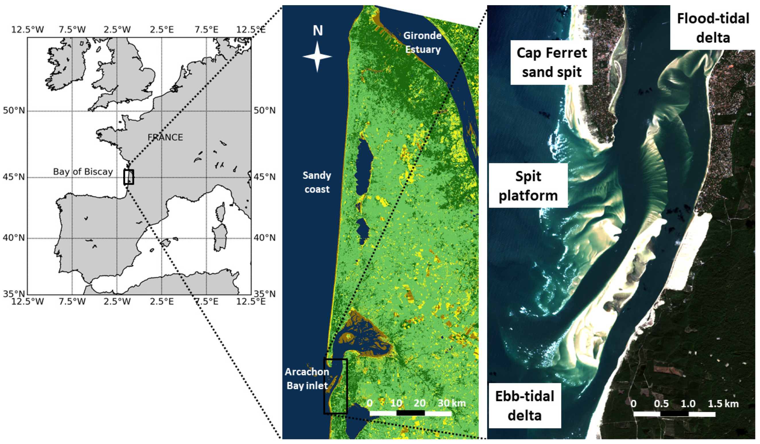
2.1. Study Area

The Arcachon Bay is a semi-enclosed lagoon of approximately 180 km2 located in SW France (44°40′ N, 1°10′ W) (Figure 1). The lagoon is connected to the Atlantic Ocean through a 10 km large tidal inlet, which disrupts the southerly longshore drift of the 110 km-long stretches of sandy coast. The inlet is a mixed energy environment [24], subject to meso- to macro-tidal conditions. The tidal range varies approximately from 1.5 m during neap tide conditions to 5 m during spring tide conditions [25]. The wave climate is energetic and strongly seasonally modulated with a monthly-averaged significant wave height Hs (peak wave period Tp), ranging from 1.1 m (8.5 s) in July with a dominant west-northwest direction to 2.4 m (13 s) in January with a dominant west direction [26]. Extreme wave conditions with the 100-year return Hs picking at 11.5 m [27] were observed during winter, where the significant wave height annually exceeds 6 m during storm events. The inlet was composed of 3 main subtidal morphological units, i.e., the spit platform, the Ebb-tidal delta, and the Flood-tidal delta, connected to a 9 m-deep northern channel and a 11 m-deep southern channel. Their morphology changes dynamically on timescales from months to years and decades [28,29].
Optical properties of seawater along the Arcachon inlet change with hydrodynamics and seasonal conditions. They were mainly controlled by the suspended particulate and colored dissolved organic matters coming from the ocean, lagoon, or adjacent coasts. The particulate organic matter (POM) was mainly dominated by phytoplankton (89% on average) and a non-negligible contribution of anthropogenic (6%) and river (5%) sources [30]. The seasonal variability of total suspended particulate matter (SPM) was controlled by river discharges and biological and hydro-sedimentary processes [31]. Over the period 2010–2020, the mean annual values of the concentration of SPM, chlorophyll-a (Chl), and particulate organic carbon to nitrogen ratio (C/N ratio, proxy of the origin of POM) were 4.95 ± 4.78 mg/L, 1.86 ± 0.79 μg/L, and 8.21 ± 20.13 mol/mol, respectively, at the station Bouée 13 located north of the inlet (statistics extracted from the data set of the French Coastal Monitoring Network SOMLIT). Maximum values of Chl (2.42 ± 1.33 μg/L) were observed in spring due to phytoplankton blooms, while maximum values of SPM (7.90 ± 7.32 mg/L) were recorded in winter due to resuspension processes. These conditions generated mildly to moderately turbid seawaters. The satellite-derived vertically averaged diffuse attenuation coefficient for downwelling irradiance (Kd) at 545 nm ranges from 0.32 to 0.79 m−1, with a mean value of 0.52 m−1 [11]. The bottom substrate of optically shallow waters, defined as seawater surfaces where the bottom significantly affects the remote sensing reflectance Rrs, was uniformly covered by medium quartz sand characterized by a cross-section ranging from 200 to 400 μm [28,32].

2.2. Ground Reference Bathymetry Data

Echo sound bathymetric data of the Arcachon Bay inlet were collected every year from April to October by the Direction Départementale des Territoires et de la Mer (DDTM) and the Syndicat Intercommunal du Bassin d’Arcachon (SIBA). These surveys were mainly carried out for the monitoring of navigation channels and the repositioning of navigation buoys; thus, bathymetric data generally covered only part of the study site. Due to the large lateral extent (almost 10 km from North to South), strong tidal currents and energetic waves, and shallow water areas (spit platform, inter-channels banks), the Arcachon inlet was a very challenging site to survey with conventional tools, which explained the lack of complete synchronous coverage. A comprehensive dataset of 450,837 echo sound data points collected between 2013 and 2020 was used in this study (Table 1). Echo sound data were acquired with an Odom Hydrotrac single-beam echosounder co-located with a Leica DGPS during low or high tide slack. The observed depths were then corrected for roll, pitch, yaw, GPS latency, and theoretical tide computed at the Arcachon-Eyrac reference tide gauge at the time of acquisition. Finally, the bathymetry (noted, Zsitu), which was associated with the corrected depth reduced within the appropriate vertical datum, was obtained after the correction of the local chart datum of the Lowest Astronomical Tide (LAT). Accuracy on Zsitu was assumed to be within 0.2 m.

2.3. Selection and Processing of Landsat-8 and Sentinel-2 Images

The Landsat-8 satellite mission was launched on 11 February 2013 by the National Aeronautics and Space Administration (NASA). Its payload comprised the Operational Land Imager (OLI) and the Thermal Infrared Sensor (TIRS). OLI provides enhanced instrument features for aquatic surface observation compared to former Landsat sensors [33]. OLI operates in the visible (VIS), near-infrared (NIR), and shortwave infrared (SWIR) for 9 spectral bands with a 12-bit radiometric resolution. Its spatial resolution was 30 m for multispectral images and 15 m for the panchromatic band. Landsat-8 Collection 1 Level 1 products were downloaded freely on https://earthexplorer.usgs.gov (accessed on 31 March 2022).
Sentinel-2A and 2B were twin polar-orbiting satellite missions launched in June 2015 and March 2017, respectively, by the European Space Agency (ESA). The multispectral instrument (MSI) mounted on the Sentinel spacecraft was very similar in design and requirements to OLI [34,35]. MSI acquired data in 13 spectral bands from VIS to SWIR with a spatial resolution ranging from 10 to 60 m and a radiometric resolution of 12 bit. Sentinel-2 Level 1C products associated with the T30TXQ tile were downloaded freely from https://scihub.copernicus.eu/ (accessed on 31 March 2022). OLI and MSI products were sufficiently consistent to be merged and to provide comprehensive observations for the monitoring of aquatic systems [36]. The combination of the products of these 3 missions yielded a global median average revisit interval of 2.9 days since the repeat cycle is 16-days for Landsat-8 and 5-days for Sentinel-2A/B [37].
SDB requires satellite images with high standards of quality, considerably reducing the number of usable images. The accuracy of SDB retrievals was strongly impacted by environmental noise caused by atmospheric and ocean surface effects [21]. Before applying atmospheric correction models, a pre-selection of satellite images was performed based on environmental criteria such as the absence of foam due to breaking waves, the absence of clouds that should not cover more than 10% of the images, and the absence of sun glint. An additional criterion of temporal proximity between bathymetry surveys and the date of image acquisition was also required, given that rapid bathymetry changes could be observed along the Arcachon inlet in response to energetic hydrodynamic conditions. For example, Capo et al. [11] demonstrated that, on average, sand bars along the Arcachon inlet migrated by about 10 m a month. Considering the spatial resolution of MSI products, only satellite images acquired within a 30-day time window of the bathymetry surveys were selected to avoid having larger bathymetric changes than the spatial resolution of images. Application of these 4 criteria to the 2013–2020 Landsat-8 and to the 2015–2020 Sentinel-2A/B archives allowed selection of 89 satellite images, among which 49 were Landsat-8 images and 40 were Sentinel-2A/B images (Figure 2a). Most of the images were acquired in October, September, April, and March (Figure 2b), when atmospheric and swell conditions (Figure 2c) were most suitable for acquiring high-quality images [38] and bathymetric field data, respectively.
In optically shallow waters, the remote sensing reflectance (Rrs) is a function of water depth, bottom albedo, and water column optical properties. Extracting Rrs from the top-of-atmosphere signal recorded by sensors requires accurate and consistent atmospheric corrections. In this study, the dark spectrum fitting atmospheric correction method (DSF), associated with the open access ACOLITE processor, was selected to process satellite images from Level-1C to Level-2A [39,40]. ACOLITE-DSF demonstrated high performance in deriving bathymetry from empirical SDB models [41]. This high performance compared to other atmospheric correction algorithms may be explained by less noisy ACOLITE products due to the assumption of spatially consistent aerosols [41,42]. Landsat-8 and Sentinel-2 A/B images were, therefore, processed to Rrs using the fixed aerosol optical thickness option for our 20 km × 20 km region of interest. Due to the large amount of bathymetry and satellite data, the sun glint correction option was not applied. All pixels contaminated by the sun glint effect were masked to avoid additional environmental noise for the assessment of the SDB empirical model performances. Finally, OLI and MSI data were projected on the same 30 m × 30 m grid to enable a joint statistical study to be carried out.

2.4. Inter-Comparison of SDB Empirical Model Performance

Three empirical approaches were selected for inter-comparison of performances. While many SDB empirical models were developed in the literature, the choice of these 3 approaches was motivated by the fact that they were representative of the 3 main well-established and emerging algorithm categories. The linear regression model (LRM) using log-transformed bands or log-transformed band ratios was originally developed by [43] and [44], and recently revisited by [41] for Sentinel-2A/B applications. The switching model (SM) [19] and the cluster-based regression model (CBR) [21] can be considered as an extension of LRM. SM was based on 2 LRM using the Red-Blue (LRM-RB) and Green-Blue (LRM-GB) log-transformed band ratios. This multi-conditional approach selects the most sensitive log-transformed band ratio for a predefined water depth range. LRM-RB was used for very shallow waters, while LRM-GB was used for deeper regions. CBR segments the region into different optical classes for which class-specific LRM were calibrated.
In practice, LRM is based on the following formulation:
Z sat   =   m 1 X   +   m 0 ,
where Zsat is the satellite-derived bathymetry (in meters) and X is the log-transformed band or log-transformed band ratio. The different parameterizations of X used in this study are log(B), log(G), log(R), log(B)/log(G), and log(R)/log(G), where B, G, and R are Rrs at the blue, green, and red bands, respectively. m0 and m1 are the coefficients of the linear regression established between the response variable Zsitu and the explanatory variable X, retrieved from a least-square approach.
The linear regression models calibrated for each satellite image have a range of application bounded by a lower limit (Zmin) and upper limit (Zmax) (Figure 3a,b). To compute Zmin and Zmax, the entire range of X values was divided into 20 intervals, bins, of equal sizes comprised between Xmin and Xmax. For each bin, the number of observations (Nbin) and the standard deviation of Zsitu values (σbin) was computed. When Nbin was lower than 30 or σbin higher than 1 m, observations of the bin were removed. The Nbin value of 30 was selected to ensure a statistical weight to the regression, while the choice of a 1 m-σbin filter was performed to remove observations associated with a strong environmental noise that generated large uncertainty on the Zsitu retrievals. The linear regression model was then calibrated from filtered observations. Zmin and Zmax were defined as the minimum and maximum values of Zsat computed from Equation (1).
SM was based on a multi-conditional procedure. In step 1, Zmax and Zmin values associated with the different parameterizations of X are computed (Figure 3c). In step 2, the calibration dataset is filtered to remove all values of Zsitu higher than the lowest Zmax values (noted Zmax-ref). In step 3, the coefficient of determination (r2) of the linear regression models calibrated for the different parameterizations of X are computed. In step 4, if the r2 value of the parameterization of X associated with Zmax-ref (noted Xref) is higher than all other X parameterization r2 values, the associated LRM is selected for the range of Zsitu values comprised between Zmin-ref and Zmax-ref. The calibration dataset is then filtered to remove all values of Zsitu lower than Zmax-ref. Xref is no longer considered in the procedure and the algorithm returns to step 2. In the opposite case, the LRM associated with Xref is not considered and the algorithm returns to step 2.
If more than one LRM is selected, a procedure of weighting is applied between Zsat values derived from the shallowest (LRM) and deepest (LRM+) models to ensure a smooth transition (Figure 3d). The lower and upper bounds of the smoothing intervals are l i m = Z max σ bin and l i m + = Z max + σ bin , respectively, where Zmax and σbin are computed from the shallowest LRM. The equation of weighting is:
Z sat   =   α   LRM   +   ( 1 α ) LRM + ,
where
α   =   ( l i m + LRM ) / ( l i m + l i m ) .
This procedure for the switching method allows for the switching points ( l i m , l i m + ) to automatically adapt when the water column optical properties change.
For the CBR method, we selected a k-means clustering algorithm for classifying each pixel into homogeneous optical classes, as in [21]. These unsupervised learning techniques showed high performance in differentiating between optically contrasted seawater classes [45,46]. The set of variables used for the classification was composed of B, G, R, and NIR was Rrs at the near-infrared band. Then, class-specific linear regression models were calibrated for each optical class using the LRM approach. To cover the optical variability of the entire study area, we selected a number of 8 optical classes. This number of classes was based on the assumption that optical conditions were controlled mainly by 3 independent environmental variables, each taking 2 outcomes, water depth (deep or shallow), sediment resuspension (yes or no), main origin of water column optical properties (ocean or lagoon), i.e., 8 possible combinations. The spatial distribution of optical classes varied from one satellite image to another, depending on hydrological conditions. One example of the distribution is presented in Figure 3f. It is important to note that pixels assigned to classes associated with optically deep waters or to classes that do not have enough Zsitu points for calibration (see the LRM procedure) will be automatically masked (Figure 3e,g).
Four statistical parameters were used to assess and compare the performance of the LRM, SM, and CBR methodologies applied to the 89 satellite images. The coefficient of determination (r2), bias (Bias), mean relative absolute difference (MRAD), and root mean square error (RMSE) were computed from the matchup dataset (DS) composed of Zsitu and its estimator Zsat. The number of observations (NDS) varies with each pair of satellite images and field bathymetry dataset. Bias, MRAD, and RMSE are computed as follows:
Bias   =   1 N DS i = 1 N DS ( Z sat ; i Z situ ; i ) ,
MRAD   =   1 N DS i = 1 N DS | Z sat ; i Z situ ; i | Z situ ; i   ×   100 % ,
MSE   =   1 N DS i = 1 N DS ( Z sat ; i Z situ ; i ) 2 .

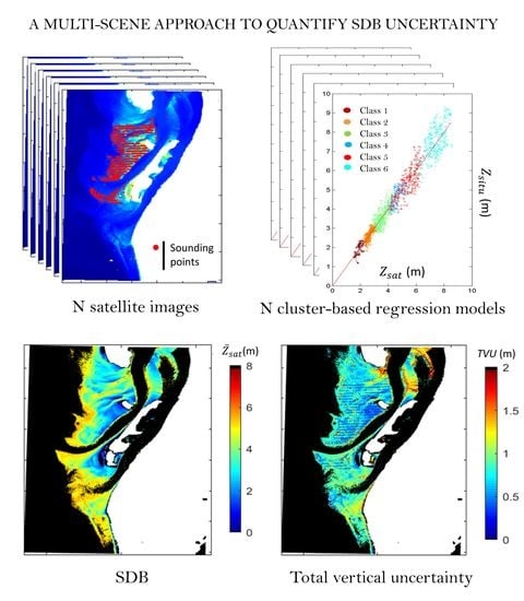
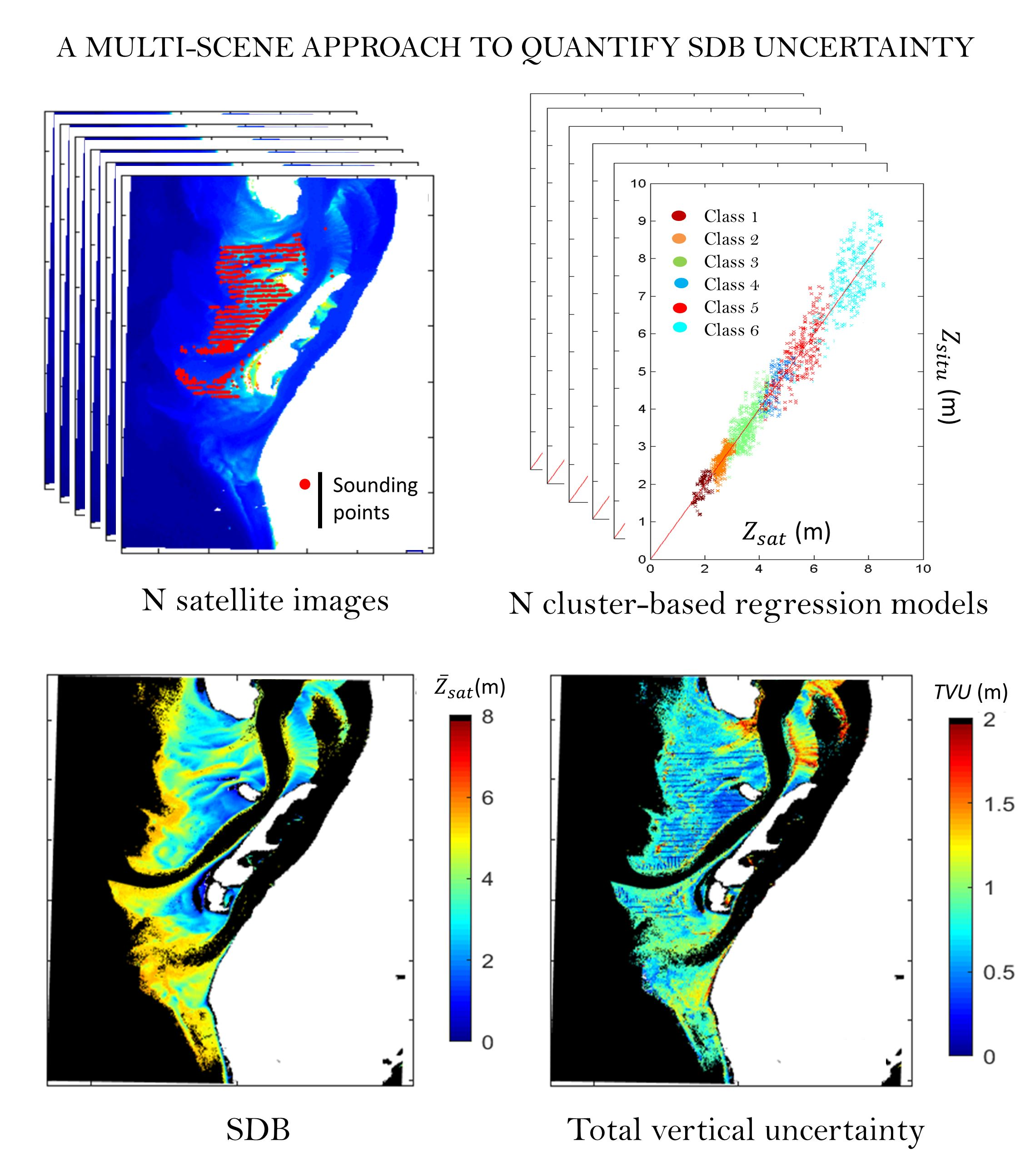
2.5. Assessment of SDB Uncertainty Using a Multi-Scene Approach

The calibration dataset often only partially covers the study area (Figure 3g). For pixels associated with areas that were not sampled and were, therefore, not included within the calibration dataset (here, referred as unsampled pixels), quantification of SDB uncertainty requires taking into account 2 terms (Figure 4). The first term was associated with the uncertainty of the SDB regression model. The second term was associated with the uncertainty generated by the extrapolation of the SDB model beyond the calibration domain. To estimate these 2 terms, an uncertainty model based on a multi-scene approach was proposed. We expressed the uncertainty as a positive value and assumed that error follows a normal distribution.
Combination of Landsat-8 and Sentinel-2 enables to have several image acquisitions in a 1 month-interval around the bathymetric survey. Assume we have N usable images for a given bathymetry survey. For each image, an SDB model was calibrated independently of other SDB models generating N bathymetry maps which can be associated with N random variables Zsat1, Zsat2, … ZsatN. Each variable was then separated into 2 parts comprising observations associated with the DS-matchup dataset, Z satj DS , and observations associated with the NS-unsampled pixels dataset, Z satj NS .
The multi-scene approach allows to define a new variable Z ¯ sat as:
Z ¯ sat   =   1 N j = 1 N Z satj DS .
Quantification of uncertainty associated with the multi-scene model requires characterizing the statistical distribution of errors over DS for different levels of bathymetry. The entire range of Z ¯ sat values were divided into bathymetry intervals of 0.5 m comprised between the minimum and maximum values. For each 0.5 meter-bin, the error term, ε bin , was computed as:
ε bin   =   Z ¯ sat Z situ .
For each bin, the normality of the ε bin distribution was tested. If the normality was rejected, observations associated with the given bin were removed. For the other bins, the bias, ε ¯ bin , was computed as the averaged value of ε bin , and the uncertainty at the 95% confidence level associated with the SDB multi-scene model was computed as:
U bin   =   1.96   ×   σ ε bin ,
where σ ε bin is the standard deviation of ε bin .
Quantification of the uncertainty associated with the extrapolation of the SDB model beyond the calibration domain was based on the model democracy theory or “one model one vote” [47]. This theory requires that variables Z sat 1 NS , Z sat 2 NS , … Z sat N NS are reasonably independent, equally plausible and that the range of model predictions represents the uncertainty in the prediction. Independence is ensured by hydrodynamic conditions, which change from one image to another, and which do not allow inference on the spatial distribution of water column optical properties. The equal plausibility criterion is controlled by a statistical test on the probability density functions that are supposed to be the same. The last criterion is controlled by a test of normality for each pixels using the Shapiro–Wilk normality test. To avoid the problem of a small sample, N should be higher than 5 if possible.
For each observation of Z sat 1 NS , Z sat 2 NS , … Z sat N NS , associated with a given pixel i of the bathymetry maps, the spread of the ensemble is computed as:
s i   =   1 N 1 j = 1 N ( Z satj ; i NS Z ¯ satj ; i NS ) 2 .
The uncertainty at the 95% confidence level associated with the true value of Z ¯ sat , i NS and generated by the extrapolation of the SDB model beyond the calibration is then given by:
U i NS   =   t N 1 ; 1 α / 2   ×   s i N ,
where t N 1 ; 1 α / 2 is the critical value found from the t-distribution table. N − 1 is the degree of freedom and α is the level of significance of the test. For a N and α value of 5 and 5%, respectively, t 4 ; 0.975 is 2.776.
Finally, the total vertical uncertainty at the 95% confidence level associated with Z situ is computed as:
T V U i NS   =   U i NS   +   U bin .
Validation of the uncertainty model was carried out from a dataset composed of 6 satellite images acquired in an interval of 1 month (S2A, 6 October 2017;_S2A, 11 October 2017;_S2A and L8, 16 October 2017;_L8, 25 October 2017; S2A, 31 October 2017) around a bathymetric survey characterized by one of the greatest spatial coverages. DS was randomly separated into 2 parts comprising a calibration dataset (DS-C) and a validation dataset (DS-V), which represented 67% and 33% of the data, respectively. DS-C allows to compute U bin , which was used to estimate T V U i NS for each observation of DS-V. DS-V allows to compute the error, ε i DS V , associated with the SDB multi-scene model for each observation as:
ε i DS V   =   Z ¯ sat , i DS V Z situ DS V .
The uncertainty model was finally evaluated by computing the percentage of absolute values of ε i DS V lower than T V U i NS . To avoid any biais due to the random extraction of a specific dataset for DS-C and DS-V, an analysis of results was conducted on 100 random samplings.

3. Results

3.1. Hydrological Conditions and Spatio-Temporal Variability of Rrs

The dataset encompasses a wide range of hydrodynamic conditions. The number of images per tidal stage (TS) varies depending on flood (N = 29), ebb (N = 26), low tide (N = 19), and high tide (N = 15) conditions (Table 2). Tidal range (TR) and tidal level (TL) data were normally distributed with a mean value of 3.10 ± 0.84 m and 2.16 ± 0.92 m, respectively. Hs ranged from 0.25 to 2.20 m, with a mean value of 1.14 ± 0.50 m. Results showed that variables TL and TS (ANOVA p-value of 1.10–11), and Season and Hs (ANOVA p-value of 0.046) were not independent. However, there was a statistical relationship between TR and TS (ANOVA p-value < 0.001), which represents a sampling bias with respect to hydrodynamic conditions. Low tide and flood were mainly associated with high TR values, while high tide and ebb show on average low TR conditions. TR was also significantly correlated with TL, with a correlation coefficient value of −0.79 (p-value < 0.001).
A principal component analysis (PCA) using the T-mode and S-mode orientations [48] was used to characterize the complexity of the spatio-temporal patterns of Rrs in the Arcachon inlet (Figure 5a). PCA was applied on G maps, as the green band was the most sensitive band for moderate values of SPM [49]. The S-mode PCA focuses on recurrent temporal patterns over space. The first principal component (PC1) explained 93.2% of the total variance. The spatial pattern associated with PC1 exhibited homogenous correlation values over the entire domain (Figure 5b). Statistical analyses performed between PC1 and environmental factors showed a significant seasonal influence with an ANOVA p-value lower than 0.001 (Table 3). The mean loading values for spring, winter, fall, and summer were 62.8, 40.0, −20.0, and −57.5, respectively. PC1 can be interpreted as describing a seasonal oscillation with high values of G in spring and winter probably associated with phytoplankton bloom and sediment resuspension processes, respectively, and low values in fall and summer.
The T-mode PCA focuses on recurrent spatial patterns over time. Results provide additional information to analyze more precisely spatial processes controlling the variability of G. The three first principal components accounted for 27.0%, 14.5%, and 6.9% of the variance. PC1 displayed an out-of-phase relationship between the G anomalies in the north and in the south (Figure 5c). A significant negative correlation was found between the PC1 and TL (p-value < 0.01) and between PC1 and TS (p-value < 0.01) (Table 3). This indicates that these anomalies of G were mainly controlled by tidal cycles. During low tide, positive anomalies of G were observed in the south associated with the downstream migration of turbid water dominated by lagoon optical properties, while negative anomalies observed during hide tide were correlated to the presence of less turbid oceanic seawater. PC2 displayed an out-of-phase relationship between the G anomalies on the western and eastern side of the channel (Figure 5d). TS significantly impacts the PC2 loadings with an ANOVA p-value lower than 0.05. The averaged loading value associated with the flood was strongly negative (−20.7), while the averaged loading value of the ebb was strongly positive (8.6). This indicates that PC2 describes a west-east oscillation of G controlled by the variation in the tidal current direction. During ebb, a strong west-east gradient of turbidity can be observed due to resuspension and advection of sediment on the eastern side of the channel. During the flood, the gradient was reversed, showing the highest turbidity values on the western side of the channel.

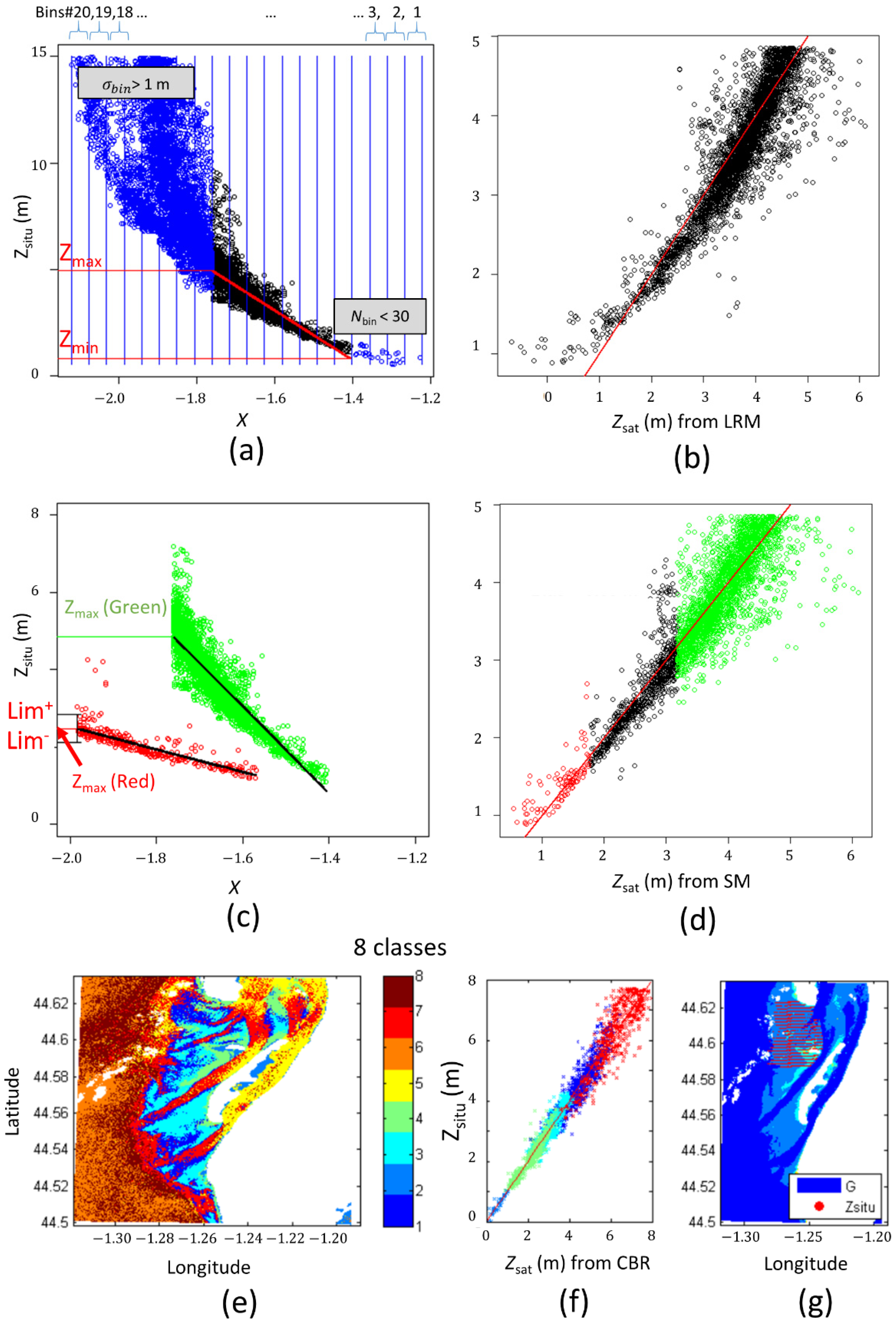
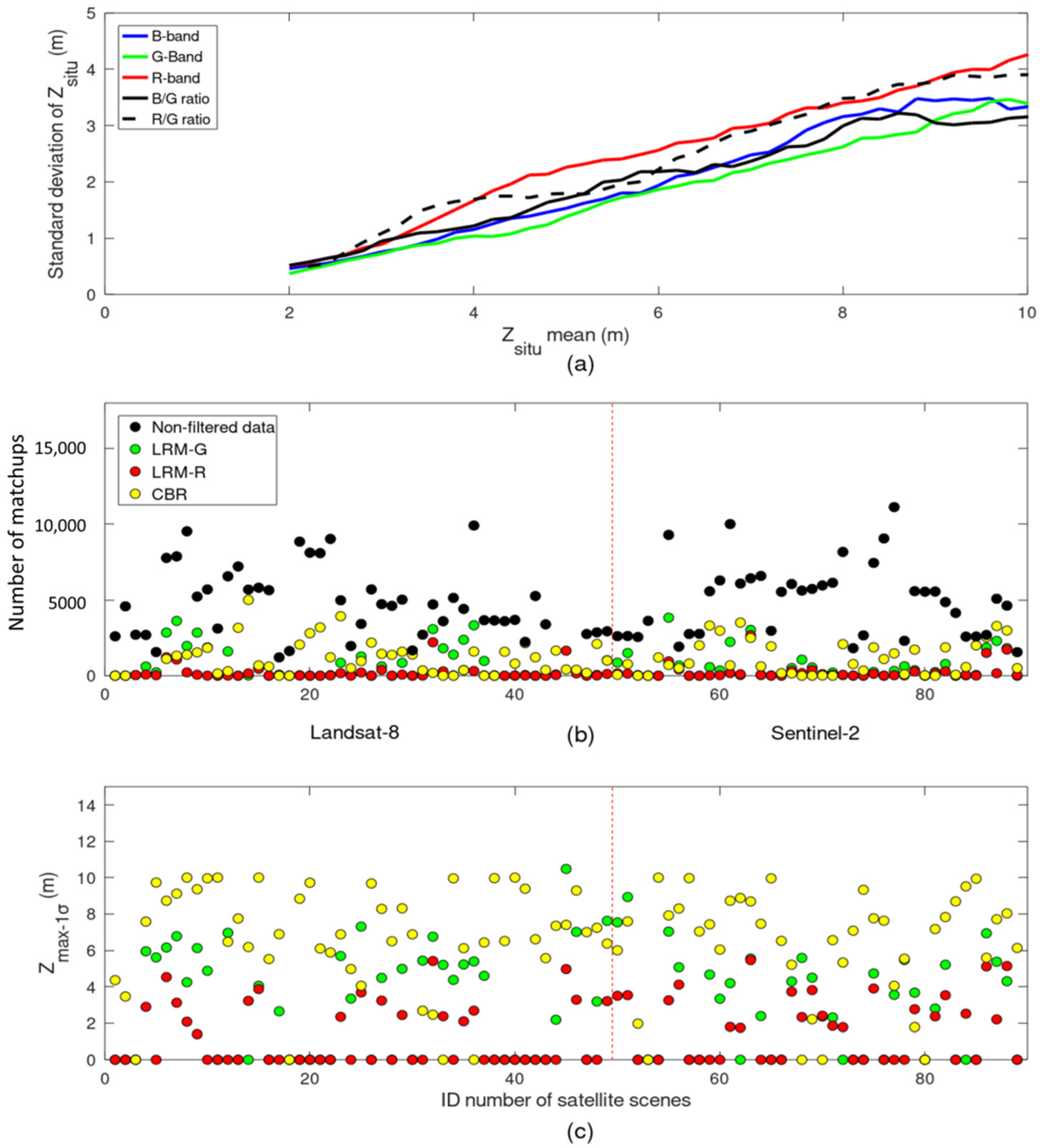
3.2. Sensitivity of Linear Regression Models to Bathymetry Changes

The sensitivity of radiometric bands or ratios to bathymetry changes can be strongly impacted by the water column optical properties, which show very specific spatial patterns associated with the hydrodynamics forcing. To analyze this sensitivity, the mean and standard deviation of Zsitu associated with the 20 X bins were computed for each image and for the different parameterizations of X. For a given value of Zsitu mean, it was assumed that the higher the standard deviation, the lower the possibility of statistically differentiating this mean value from other means and, therefore, the lower the sensitivity.
Standard deviations associated with the G-band were lower than for the other X parameterizations, except for bathymetric values deeper than 9 m (Figure 6a). On the other hand, R-band showed the highest standard deviations except for bathymetric values that ranged from 2 m to 2.5 m. For G-band, the standard deviation was less than 1 m for all bathymetry lower than 4.4 m. This value decreased to 4.1 m, 3.8 m, 3.4 m, and 3.2 m, for B-band, B/G ratio, R-band, and R/G ratio, respectively. B-band and R-band showed a lower sensitivity than the G-band. This confirms a comprehensive sensitivity analysis carried out prior to this study, which demonstrates that the best performance for LRM and CBR was obtained by using G-band, while for SM, it was obtained by using the combination of R-band and G-band. In the following, the presentation of LRM, SM, and CBR results will be focused only on these X parameterizations.
When the filter of 1σ was applied to the calibration dataset, the number of matchups significantly decreased from 915,326 points to 337,607 points, 130,583 points, and 19,737 points, for CBR, LRM using the log-transformed G-band (LRM-G), and LRM using the log-transformed R-band (LRM-R) methods, respectively (Figure 6b). A total of 70 satellite images had more than 100 matchups for CBR, whereas LRM-G and LRM-R had only 44 and 31 satellite images, respectively. It was interesting to note that the number of satellites images with more than 1000 and 10,000 matchups for CBR filter, was 43 and 3, respectively. Satellite images with few match-ups generated a 1σ-filtered maximum bathymetry (Zmax−1σ) value of 0. For CBR, 80 satellite scenes show a Zmax−1σ value different of 0 (Figure 6c). The mean value of Zmax−1σ was 7.3 ± 2.1 m. For LRM-G and LRM-R, the mean values were 5.1 ± 1.7 m and 3.2 ± 1.1 m, with a total number of images of 50 and 39, respectively.
Data filtering for CBR approach was applied on the different class-specific LRM-G. Each class was associated with specific optical conditions. The use of these classes allowed us to split the initial matchup dataset into class-specific matchup datasets for which the natural variability in the relationships between X and Zsitu was significantly reduced. This reduction of variability allowed us to reduce the number of matchups removed by the 1σ-filter.

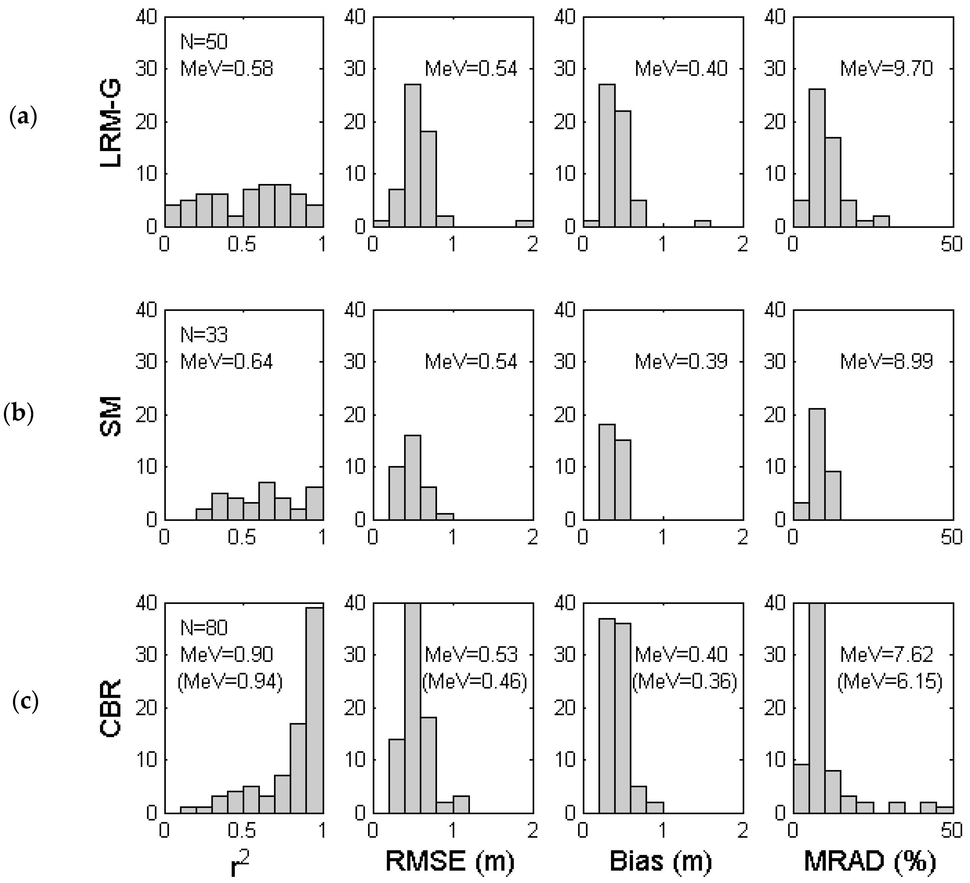
3.3. Inter-Comparison of the Performance of Empirical SDB Approaches

The performance of the LRM-G approach was evaluated using the 50 satellite images for which the Zmax−1σ value was different than 0. The median values for r2, RMSE, Bias, and MRAD were 0.58, 0.54 m, 0.40 m, and 9.70%, respectively (Figure 7). The performance of SM using LRM-G and LRM-R was evaluated using a reduced dataset of 33 satellite images for which the Zmax−1σ value was different than 0 for G-band and R-band. SM performance was slightly higher than LRM-G performance. The median values for r2, RMSE, Bias, and MRAD were 0.64, 0.54 m, 0.39 m, and 8.99%, respectively. The CRB approach allowed us to evaluate the performance using a significantly larger dataset (N = 80). The median values for r2, RMSE, Bias, and MRAD were 0.90, 0.53 m, 0.40 m, and 7.62%, which demonstrated higher performance than LRM-G and SA. When the analysis focused on a reduced dataset of the 33 best satellite scenes, performance became significantly higher. The median values for r2, RMSE, Bias, and MRAD were 0.94, 0.46 m, 0.36 m, and 6.15%.

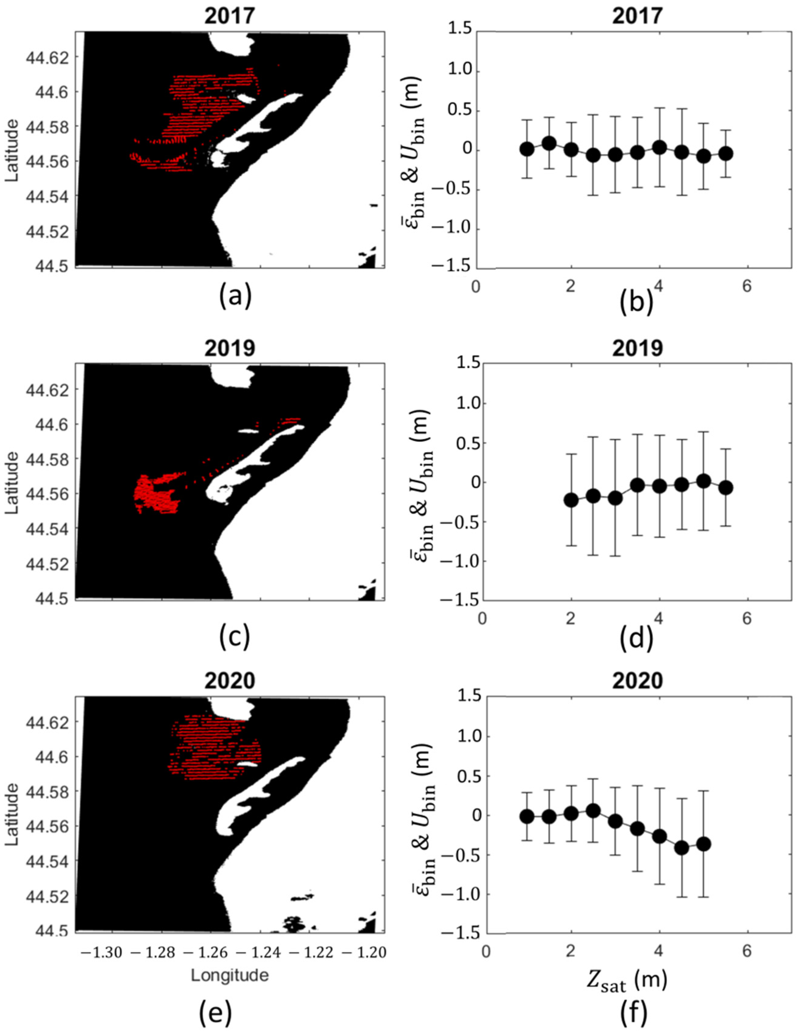
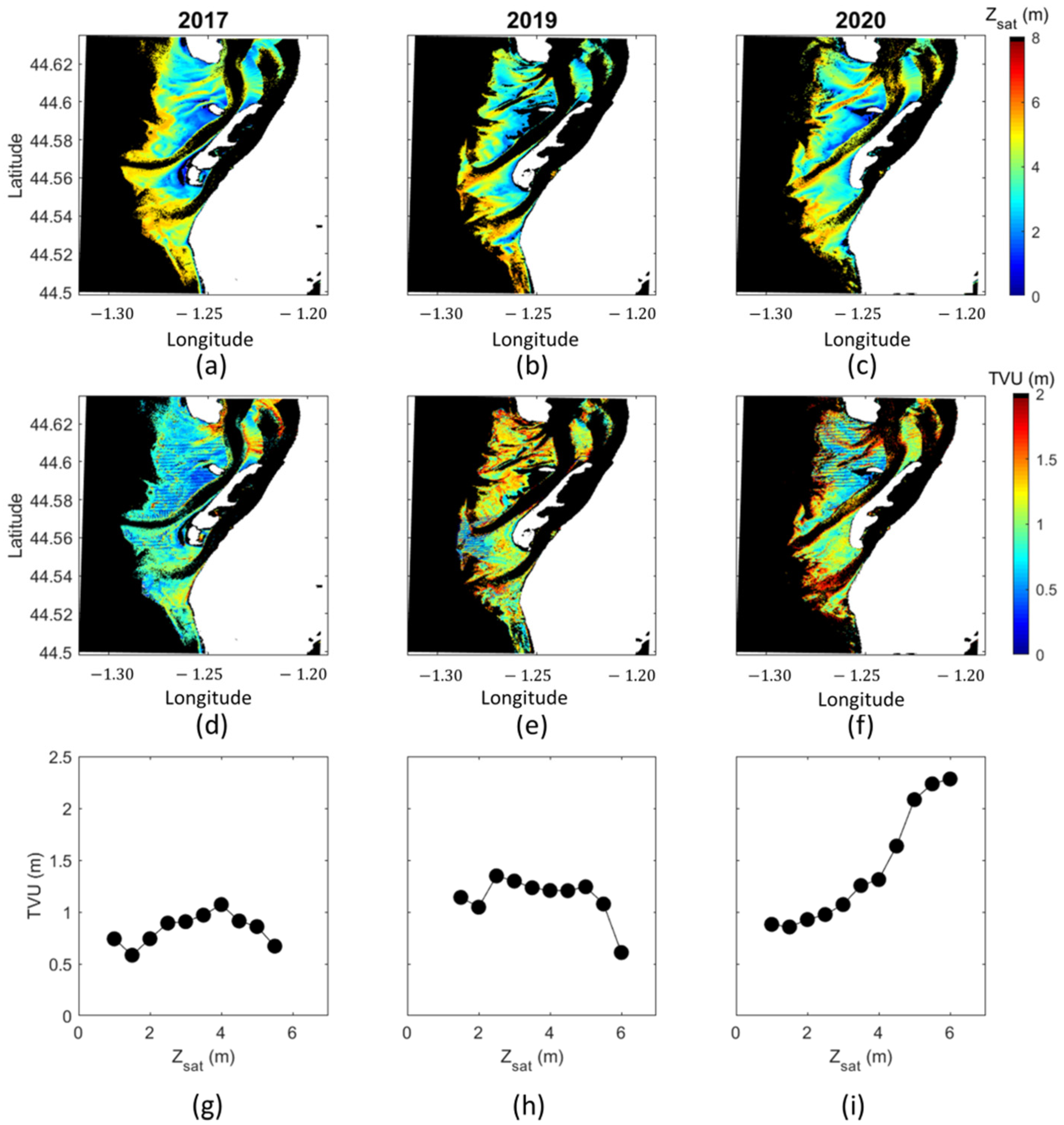
3.4. Validation of the SDB Uncertainty Model

Validation of the multi-scene SDB uncertainty model was carried out only for the CBR approach that showed the best performance for regression models and allowed exploiting more satellite images and generating bathymetry maps over a larger depth range. After applying the 1σ-filter, the matchup dataset (DS), associated with the six satellite images acquired in October 2017, was composed of 3188 sounding points. The random point extraction procedures generated a calibration dataset (DS-C) and a validation dataset (DS-V) composed of 2136 and 1052 points, respectively (Figure 8a). The percentage of observations associated with an SDB error lower than the total vertical uncertainty, P( ε i DS V < TVUi), was computed for each of the 100 random samplings (Figure 8b). The absolute frequency of P( ε i DS V < TVUi) displayed a normal distribution with a mean value of 95.8% and a standard deviation of 0.5%. The minimum and maximum values were 94.6% and 97.2%, respectively. 90% of the P( ε i DS V < TVUi) values were comprised between 95.1% and 96.7%. Only five samplings showed a value lower than 95%, indicating that the risk of failure of our multi-scene SDB uncertainty model was less than 5%.

4. Discussion

4.1. Impact of the Multi-Scene Approach on Uncertainty

Three periods of 1 month each were identified to derive SDB and uncertainty maps from the multi-scene approach. The first period in October 2017 was covered by six satellite images. The second and third periods were centered on the months of September 2019 and September 2020, including, respectively, five and four satellite images of high quality. Field bathymetry datasets associated with these two last periods were composed of 2148 and 2802 sounding points, respectively. In comparison to the 2017 bathymetric survey, the spatial distributions of the bathymetric data points in 2019 and 2020 were smaller (Figure 9a,c,e). In 2020, field bathymetry data were mainly located on the spit platform, while the data collected in 2020, were gathered along the southern part of the inlet. Consequently, the bathymetry acquired in 2017, 2019, and 2020 showed different frequency distributions with median values of 3.8 m, 4.3 m, and 3.3 m, respectively.
The bias ( ε ¯ bin ) and the 95% uncertainty associated with CBR ( U bin ) were computed from DS for each 0.5 m bins (Figure 9b,d,f). ε ¯ bin showed well-distributed values around zero, indicating the good performance of linear regressions. The average values of ε ¯ bin for 2017, 2019, and 2020, were −0.02 m, −0.03 m, and −0.07 m, respectively. It can be noted that in 2020, ε ¯ bin showed a significant deviation from zero for bathymetry higher than 3.5 m. This deviation was due to the low number of observations for these bathymetry ranges. The average values of U bin computed from Z ¯ sat were 0.67 m, 0.94 m, and 0.67 m in 2017, 2019, and 2020, respectively. When U bin were computed from Z satj , with j ranging from 1 to N, the general mean values of U bin were 1.0 m, 1.54 m, and 0.96 m, respectively. These results highlighted that the multi-scene approach allowed us to significantly reduce the 95% uncertainty associated with the SDB regression models.

4.2. Impact of the Spatial Distribution of Sounding Point on Uncertainty

SDB and uncertainty maps, generated from the multi-scene approach, for the three 1-month time periods are presented in Figure 10. Most of the study site area was covered by the SDB models (Figure 10a–c), except for optically deep regions (ocean and tidal channels). The TVU map of 2017 shows values lower or equal to 1 m, except for the northern section of the inlet inner part where more turbid seawaters could generate higher uncertainties (Figure 10d). In 2019 and 2020, areas with uncertainties higher than 1 m (Figure 10e,f) showed larger cumulative surfaces than the ones in 2017. The mean values of TVU for each bin of Z sat were displayed for the three years (Figure 10g–i). The average values were 0.89, 1.21, and 1.41 m, respectively. In 2017, all TVU averaged values were lower than 1.1 m, with a minimum observed for bathymetric values ranging from 1 to 1.5 m and a maximum value for the ones ranging from 4 to 4.5 m. In 2019, the maximum value of TVU was observed for bathymetric values comprised between 2 and 2.5 m, while the minimum value was observed for deeper waters. In 2020, the maximum TVU values were observed for deeper waters. These results may directly be associated with the specific spatial distribution of sounding points in 2019 and 2020, reducing the quality of the representativeness of the calibration dataset.
To better illustrate the impact of the spatial distribution of sounding points on the uncertainty model performance, three examples of the contrasted spatial distribution of sounding points for the 2017 dataset are discussed (Figure 11a). The first case (case 1) was associated with a spatially homogeneous point extraction from DS. One point out of three was extracted in order to generate DS-V. This selection ensured that DS-C was optically representative of DS-V. The second (case 2) and third (case 3) cases were associated with a geographic segmentation of DS-C and DS-V. For case 2, DS-C points were located on the northern part of the study area, while DS-C points were located on the southern part of the study area for case 3. These configurations may potentially affect the representativeness of the optical variability associated with DS-C, as the largest SDB errors, ε bin , in DS were located in the northeast section of the study area. This specific distribution of ε bin was due to a strong east-west optical gradient controlled by the tidal current direction.
ε i DS V and TVUi values were computed for each observation of DS-V for the three different cases (Figure 11b). Case 1 showed a P( ε i DS V < TVUi) value of 95.8% was equal to the mean value of P( ε i DS V < TVUi) computed over the 100 random samplings. For case 2, P( ε i DS V < TVUi) showed a value of 97.7%, significantly higher than the maximum previously observed for the 100 random samplings. This case was a favorable configuration of the spatial distribution of sounding points. The risk of ε i DS V being greater than TVUi was less than 5%. This result was due to lower optical variability in DS-V than in DS-C, which leads to overestimating U bin and finally, TVUi. Case 3 was the opposite configuration. The high optical variability associated with DS-V was not taken into account in DS-C and led to significantly underestimated U bin . In this unfavorable scenario, 10.1% of observations had a ε i DS V value greater than TVUi. However, this result should not be interpreted as a limitation of the uncertainty model but rather as a limitation of the classification approach selected in the CBR approach. Observations in DS-V associated with the strongest errors were classified among the classes that contained observations of DS-C despite a low spectral similarity. For future research, an alternative to the k-means clustering algorithm would be a fuzzy-c means clustering approach, which quantifies the performance of the pixels classification in relation to their optical properties [50,51]. Another alternative would be a supervised approach based, for example, on a random forests classifier [16]. This technique provides an accuracy map for the classification, which contains the indicator of the confidence degree of the classification.

4.3. Morphodynamics Application

SDB maps offer a unique opportunity to study morphological changes of large-scale tidal inlets, such as the Arcachon inlet, including the migration of sandbars, shoals, and tidal ebb and flood deltas. These maps can be used in semi-quantitative way by analyzing the longitudinal and latitudinal changes of specific isobaths. An example of the comparison between two isobaths (3 m and 4 m deep) extracted from SDB maps in 2017 and 2019 (Figure 12a–c) shows a southward migration of the ebb tidal delta and the formation of a large sandbar on the adjacent coast (−1.27°, 44.53°). The analysis of these morphological changes analyzed from SDB maps spanning years to decades supports the comprehensive understanding of the multi-annual dynamics of tidal inlet and the adjacent coast over relatively large spatial scales [52]. The supplementary use of uncertainty maps offers the opportunity to consider the analysis of vertical and volumetric morphological changes observed along the tidal inlet. The comparison of the 2017 and 2019 SDB maps (Figure 12d) showed that absolute vertical changes ranged from 0 to 4 m, while the sum of the uncertainties of 2017 and 2019 ranged from 0 to 3 m (Figure 12e). Despite high TVU values in 2019 due to low representativeness of the calibration dataset, several regions showed lower uncertainty values than bathymetric changes (Figure 12f). This result allows these changes to be assigned a high degree of confidence. For other regions, uncertainties were in the same order of magnitude as the vertical changes. However, they were meant to be significantly reduced in the future with the increase in the number and quality of the satellite images, along with enhancements of the bathymetry survey strategies and SDB algorithms.

5. Conclusions

In this study, the objectives are to evaluate the performance and robustness of well-established SDB empirical models and to propose and validate an uncertainty model for a mixed energy coastal environment. Uncertainty estimation provides new fundamental information for assessing the interpretability of SBDs and new perspectives for the use of these types of maps for the analysis of large-scale coastal systems.
The Arcachon lagoon inlet is characterized by a high spatial and temporal variability of water column optical properties mainly controlled by hydrodynamics and seasonal conditions. The CBR approach is the most appropriate approach to exploit the greatest number of images over the largest depth range and to reduce the natural optical variability of class-specific regression models, providing better performance and robustness than the other methods.
The total vertical uncertainty (TVU) associated with SDB empirical models depends on both the uncertainty generated by the regression model and the uncertainty due to the extrapolation of the SDB model beyond the calibration domain. The multi-scene approach developed in this study allows us to significantly reduce the uncertainty related to the regression models. The uncertainty associated with out-of-scope optical conditions is sensitive to the sampling of optical variability of the study area and consequently to the spatial distribution of sounding points. Furthermore, this component of TVU is impacted by the number of satellite images used for the multi-scene approach and by the associated hydrodynamic conditions. In the context of multisource bathymetric data merging approaches, these results demonstrate the need to adapt the sampling strategy of sounding points of bathymetric surveys to the optical conditions of the water column in order to generate a calibration dataset representative of the optical variability of the study site.

Author Contributions

Conceptualization, B.L. and O.B.; data curation, B.L. and A.N.L.; formal analysis, B.L. and O.B.; funding acquisition, A.N.L. and N.S.; investigation, B.L. and O.B.; methodology, B.L. and O.B.; project administration, A.N.L. and N.S.; supervision, B.L.; validation, B.L., O.B., A.N.L. and N.S.; writing—original draft, B.L. and O.B.; writing—review and editing, B.L., O.B., A.N.L. and N.S. All authors have read and agreed to the published version of the manuscript.

Funding

This research is part of the ARCADE project and was co-funded by the Region Nouvelle-Aquitaine, the Parc Naturel Marin du Bassin d’Arcachon, the Agence de l’Eau Adour-Garonne, the Syndicat Intercommunal du Bassin d’Arcachon, the Bureau de Recherches Géologiques et Minières and the Institut Français de Recherche pour l’Exploitation de la Mer.

Institutional Review Board Statement

Not applicable.

Informed Consent Statement

Not applicable.

Data Availability Statement

Landsat-8 Collection 1 Level 1 products were downloaded freely on https://earthexplorer.usgs.gov accessed on 16 March 2022. Sentinel-2 Level 1C products associated with the T30TXQ tile were downloaded freely from https://scihub.copernicus.eu/ accessed on 16 March 2022. Bathymetry data can be ordered from the Direction Départementale des Territoires et de la Mer 33 and the Syndicat Intercommunal du Bassin d’Arcachon (France).

Acknowledgments

The authors would like to thank the Direction Départementale des Territoires et de la Mer 33 and the Syndicat Intercommunal du Bassin d’Arcachon for kindly providing the bathymetric datasets. This research also significantly benefited from the high-quality of open-access satellite imagery provided by the European Space Agency (Sentinel-2 images) and the United States Geological Survey (Landsat-7 and Landsat-8 images).

Conflicts of Interest

The authors declare no conflict of interest. The funders had no role in the design of the study; in the collection, analyses, or interpretation of data; in the writing of the manuscript, or in the decision to publish the results.

References

  1. Newton, A.; Weichselgartner, J. Hotspots of coastal vulnerability: A DPSIR analysis to find societal pathways and responses. Estuar. Coast. Shelf Sci. 2014, 140, 123–133. [Google Scholar] [CrossRef]
  2. Nicholls, R.J.; Wong, P.P.; Burkett, V.R.; Woodroffe, C.D.; Hay, J.E. Climate change and coastal vulnerability assessment: Scenarios for integrated assessment. Sustain. Sci. 2008, 3, 89–102. [Google Scholar] [CrossRef]
  3. Ranasinghe, R. Assessing climate change impacts on open sandy coasts: A review. Earth-Sci. Rev. 2016, 160, 320–332. [Google Scholar] [CrossRef] [Green Version]
  4. Benveniste, J.; Cazenave, A.; Vignudelli, S.; Fenoglio-Marc, L.; Shah, R.; Almar, R.; Andersen, O.; Birol, F.; Bonnefond, P.; Bouffard, J.; et al. Requirements for a Coastal Hazards Observing System. Front. Mar. Sci. 2019, 6, 348:1–348:24. [Google Scholar] [CrossRef] [Green Version]
  5. Lebbe, T.B.; Rey-Valette, H.; Chaumillon, E.; Camus, G.; Almar, R.; Cazenave, A.; Claudet, J.; Rocle, N.; Meur-Férec, C.; Viard, F.; et al. Designing coastal adaptation strategies to tackle sea level rise. Front. Mar. Sci. 2021, 8, 740602:1–740602:13. [Google Scholar] [CrossRef]
  6. International Hydrographic Organization. International Hydrographic Publication C-55 Status of Hydrographic Surveying and Charting Worldwide. 2022. Available online: https://iho.int/uploads/user/pubs/cb/c-55/c55.pdf (accessed on 11 March 2022).
  7. Jacob, B.; Stanev, E.V. Understanding the impact of bathymetric changes in the German bight on coastal hydrodynamics: One step toward realistic morphodynamic model. Front. Mar. Sci. 2021, 8, 640214:1–640214:18. [Google Scholar] [CrossRef]
  8. Honegger, D.A.; Haller, M.C.; Holman, R.A. High-resolution bathymetry estimates via X-band marine radar: 1. beaches. Coastal Eng. 2019, 149, 39–48. [Google Scholar] [CrossRef]
  9. Cesbron, G.; Melet, A.; Almar, R.; Lifermann, A.; Tullot, D.; Crosnier, L. Pan-european sateliite-derived coastal bathymetry—Review, user needs and future services. Front. Mar. Sci. 2021, 8, 740830:1–740830:15. [Google Scholar] [CrossRef]
  10. Holman, R.; Plant, N.; Holland, T. cBathy: A robust algorithm for estimating nearshore bathymetry. J. Geophys. Res. 2013, 118, 2595–2609. [Google Scholar] [CrossRef]
  11. Capo, S.; Lubac, B.; Marieu, V.; Robinet, A.; Bru, D.; Bonneton, P. Assessment of the decadal morphodynamic evolution of a mixed energy inlet using ocean color remote sensing. Ocean Dyn. 2014, 64, 1517–1530. [Google Scholar] [CrossRef]
  12. Maritorena, S.; Morel, A.; Gentili, B. Diffuse reflectance of oceanic shallow waters: Influence of water depth and bottom albedo. Limnol. Oceanogr. 1994, 39, 1689–1703. [Google Scholar] [CrossRef]
  13. Lee, Z.P.; Carder, K.L.; Mobley, C.D.; Steward, R.G.; Patch, J.F. Hyperspectral remote sensing for shallow waters: II deriving bottom depths and water properties by optimization. Appl. Opt. 1999, 38, 3831–3843. [Google Scholar] [CrossRef] [PubMed] [Green Version]
  14. Honegger, D.A.; Haller, M.C.; Holman, R.A. High-resolution bathymetry estimates via X-band marine radar: 2. Effects of currents at tidal inlets. Coastal Eng. 2020, 156, 103626–103643. [Google Scholar] [CrossRef]
  15. Lyzenga, D.R. Passive remote sensing techniques for mapping water depth and bottom features. Appl. Opt. 1978, 17, 379–383. [Google Scholar] [CrossRef]
  16. Wei, C.; Zhao, Q.; Lu, Y.; Fu, D. Assessment of empirical algorithms for shallow water bathymetry using multi-spectral imagery of Pearl River delta coast, china. Remote Sens. 2021, 13, 3123. [Google Scholar] [CrossRef]
  17. Dekker, A.G.; Phinn, S.R.; Anstee, J.; Bissett, P.; Brando, V.E.; Casey, B.; Fearns, P.; Hedley, J.; Klonowski, W.; Lee, Z.P.; et al. Intercomparison of shallow water bathymetry, hydro-optics, and benthos mapping techniques in australian and caribbean coastal environments. Limnol. Oceanogr. Methods 2011, 9, 396–425. [Google Scholar] [CrossRef] [Green Version]
  18. Wei, J.; Wand, M.; Lee, Z.; Briceno, H.O.; Yu, X.; Jiang, L.; Garcia, R.; Wang, J.; Luis, K. Shallow water bathymetry with multi-spectral satellite ocean color sensors: Leveraging temporal variation in image data. Remote Sens. Environ. 2020, 250, 112035–112050. [Google Scholar] [CrossRef]
  19. Botha, E.; Brando, V.; Dekker, A.; Botha, E.J.; Brando, V.E.; Dekker, A.G. Effects of per-pixel variability on uncertainties in bathymetric retrievals from high-resolution satellite images. Remote Sens. 2016, 8, 459. [Google Scholar] [CrossRef] [Green Version]
  20. Caballero, I.; Stumpf, R. Towards routine mapping of shallow bathymetry in environments with variable turbidity: Contribution of Sentinel-2A/B satellites mission. Remote Sens. 2020, 12, 451. [Google Scholar] [CrossRef] [Green Version]
  21. Geyman, E.C.; Maloof, A.C. A simple method for extracting water depth from multispectral satellite imagery in regions of variable bottom type. Earth Space Sci. 2019, 6, 527–537. [Google Scholar] [CrossRef]
  22. International Hydrographic Organization. International Hydrographic Publication C-44 Standards for Hydrographic Surveys Edition 6.0.0. 2020. Available online: https://iho.int/uploads/user/pubs/standards/s-44/S-44_Edition_6.0.0_EN.pdf (accessed on 30 September 2020).
  23. IOCCG. Uncertainties in Ocean Colour Remote Sensing; Mélin, F., Ed.; IOCCG Report series, No. 18; International Ocean-Colour Coordinating Group: Dartmouth, NS, Canada, 2019; ISBN 978-1-896246-68-0. [Google Scholar]
  24. Hayes, M.O. Barrier island morphology as a function of tidal and wave regime. In Barrier Island; Leatherman, S.P., Ed.; Academic Press: New York, NY, USA, 1979; pp. 1–28. ISBN 0-12-440260-7. [Google Scholar]
  25. Senechal, N.; Sottolichio, A.; Bertrand, F.; Goeldner-Gianella, L.; Garlan, T. Observations of waves’ impact on currents in a mixed-energy tidal inlet: Arcachon on the southern French Atlantic coast. J. Coast. Res. 2013, 65, 2053–2058. [Google Scholar] [CrossRef]
  26. Castelle, B.; Bujan, S.; Ferreira, S.; Dodet, G. Foredune morphological changes and beach recovery from the extreme 2013/2014 winter at a high-energy sandy coast. Mar. Geol. 2017, 385, 41–55. [Google Scholar] [CrossRef]
  27. Nicolae Lerma, A.; Bulteau, T.; Lecacheux, S.; Idier, D. Spatial variability of extreme wave height along the Atlantic and channel French coast. Ocean Eng. 2015, 97, 175–185. [Google Scholar] [CrossRef]
  28. Cayocca, F. Long-term morphological modeling of a tidal inlet: The Arcachon Basin, France. Coast. Eng. 2001, 42, 115–142. [Google Scholar] [CrossRef]
  29. Nahon, A.; Idier, D.; Sénéchal, N.; Mallet, C.; Mugica, J. Imprints of wave climate and mean sea level variations in the dynamics of a coastal spit over the last 250 years: Cap Ferret, SW France. Earth Surf. Process. Landf. 2019, 44, 2112–2125. [Google Scholar] [CrossRef]
  30. Liénart, C.; Savoye, N.; Bozec, Y.; Breton, E.; Conan, P.; David, V.; Feunteun, E.; Grangeré, K.; Kerhervé, P.; Lebreton, B.; et al. Dynamics of particulate organic matter composition in coastal systems: A spatio-temporal study at multi-systems scale. Prog. Oceanogr. 2017, 156, 221–239. [Google Scholar] [CrossRef] [Green Version]
  31. Glé, C.; Del Amo, Y.; Sautour, B.; Laborde, P.; Chardy, P. Variability of nutrients and phytoplankton primary production in a shallow macrotidal coastal ecosystem (Arcachon Bay, France). Estuar. Coast. Shelf Sci. 2008, 76, 642–656. [Google Scholar] [CrossRef]
  32. Pedreros, R.; Howa, H.L.; Michel, D. Application of grain size trend analysis for the determination of sediment transport pathways in intertidal areas. Mar. Geol. 1996, 135, 35–49. [Google Scholar] [CrossRef] [Green Version]
  33. Pahlevan, N.; Lee, Z.; Hu, C.; Schott, J.R. Diurnal remote sensing of coastal/oceanic waters: A radiometric analysis for geostationary coastal and air pollution events. Appl. Opt. 2014, 53, 648–665. [Google Scholar] [CrossRef]
  34. Drusch, M.; del Bello, U.; Carlier, S.; Colin, O.; Fernandez, V.; Gascon, F.; Hoersch, B.; Isoal, C.; Laberinti, P.; Martimort, P.; et al. Sentinel-2: ESA’s Optical High-Resolution Mission for GMES Operational Services. Remote Sens. Environ. 2012, 120, 25–36. [Google Scholar] [CrossRef]
  35. Pahlevan, N.; Scott, J.R.; Franz, B.A.; Zibordi, G.; Markham, B.; Bailey, S.; Schaaf, C.B.; Ondrusek, M.; Greb, S.; Strait, C.M. Landsat 8 remote sensing reflectance (Rrs) products: Evaluations, intercomparisons, and enhancements. Remote Sens. Environ. 2017, 190, 289–301. [Google Scholar] [CrossRef]
  36. Pahlevan, N.; Chittimalli, S.K.; Balasubramaniam, S.V.; Velluci, V. Sentinel-2/Landsat-8 product consistency and implications for monitoring aquatic systems. Remote Sens. Environ. 2019, 220, 19–29. [Google Scholar] [CrossRef]
  37. Li, J.; Chen, B. Global revisit interval analysis of Landsat-8-9 and Sentinel-2A -2B data for terrestrial monitoring. Sensors 2020, 20, 6631. [Google Scholar] [CrossRef]
  38. Bru, D.; Lubac, B.; Normandin, C.; Robinet, A.; Leconte, M.; Hagolle, O.; Martiny, N.; Jamet, C. Atmospheric correction of multi-spectral littoral images using a PHOTONS/AERONET-based regional aerosol model. Remote Sens. 2017, 9, 814. [Google Scholar] [CrossRef] [Green Version]
  39. Vanhellemont, Q.; Ruddick, K. Atmospheric correction of metre-scale optical satellite data for inland and coastal water applications. Remote Sens. Environ. 2018, 216, 586–597. [Google Scholar] [CrossRef]
  40. Vanhellemont, Q. Sensitivity analysis of the dark spectrum fitting atmospheric correction for metre- and decametre-scale satellite imagery using autonomous hyperspectral radiometry. Opt. Express 2020, 28, 29948–29965. [Google Scholar] [CrossRef]
  41. Caballero, I.; Stumpf, R.P. Retrieval of nearshore bathymetry from Sentinel-2A and 2B satellites in South Florida coastal waters. Estuar. Coast. Shelf Sci. 2019, 12, 451–474. [Google Scholar] [CrossRef]
  42. Vanhellemont, Q.; Ruddick, K. Atmospheric correction of Sentinel-3/OLCI data for mapping of suspended particulate matter and chlorophyll-a concentration in Belgian turbid coastal waters. Remote Sens. Environ. 2021, 256, 112284. [Google Scholar] [CrossRef]
  43. Lyzenga, D.R. Remote sensing of bottom reflectance and water attenuation parameters in shallow water using aircraft and Landsat data. Int. J. Remote Sens. 1981, 2, 71–82. [Google Scholar] [CrossRef]
  44. Stumpf, R.P.; Holderied, K.; Sinclair, M. Determination of water depth with high-resolution satellite imagery over variable bottom types. Limnol. Oceanogr. 2003, 48, 547–556. [Google Scholar] [CrossRef]
  45. Lubac, B.; Loisel, H. Variability and classification of remote sensing reflectance spectra in the eastern English Channel and southern North Sea. Remote Sens. Environ. 2007, 110, 45–58. [Google Scholar] [CrossRef]
  46. Vantrepotte, V.; Loisel, H.; Dessailly, D.; Mériaux, X. Optical classification of contrasted coastal waters. Remote Sens. Environ. 2012, 123, 306–323. [Google Scholar] [CrossRef]
  47. Knutti, R.; Hadorn, G.H.; Baumberger, D. Uncertainty Quantification Using Multiple Models—Prospects and Challenges. In Computer Simulation Validation: Fundamental Concepts, Methodological Frameworks, and Philosophical Perspectives; Beisbart, C., Saam, N.J., Eds.; Springer: Cham, Switzerland, 2019; pp. 835–855. [Google Scholar] [CrossRef]
  48. Normandin, C.; Lubac, B.; Sottolichio, A.; Frappart, F.; Ygorra, B.; Marieu, V. Analysis of suspended sediment variability in a large highly turbid estuary using a 5-year-long remotely sensed data archive at high resolution. J. Geophys. Res. Oceans 2019, 124, 7661–7682. [Google Scholar] [CrossRef] [Green Version]
  49. Novoa, S.; Doxaran, D.; Ody, A.; Vanhellemont, Q.; Lafon, V.; Lubac, B.; Gernez, P. Atmospheric corrections and multiconditional algorithm for multi-sensor remote sensing of suspended particulate matter in low-to-high turbidity levels coastal waters. Remote Sens. 2017, 9, 61. [Google Scholar] [CrossRef] [Green Version]
  50. Moore, T.S.; Campbell, J.W.; Feng, H. A fuzzy logic classification scheme for selecting and blending satellite ocean color algorithms. IEEE Trans. Geosci. Remote Sens. 2001, 39, 1764–1776. [Google Scholar] [CrossRef]
  51. Jackson, T.; Sathyendranath, S.; Mélin, F. An improved optical classification scheme for the Ocean Colour Essential Climate Variable and its applications. Remote Sens. Environ. 2017, 203, 152–161. [Google Scholar] [CrossRef]
  52. Burvingt, O.; Nicolae Lerma, A.; Lubac, B.; Mallet, C.; Senechal, N. Geomorphological control of sandy beaches and dunes alongside a mixed-energy tidal inlet. Mar. Geol. 2022; accepted. [Google Scholar]
Figure 1. The Arcachon Bay inlet located south of the Gironde estuary at the end of the 110 km-long linear Gironde sandy coast (SW France). The three main morphological units of the study area are the spit platform connected to the Cap Ferret sand spit, the edd-tidal, and the flood-tidal deltas.
Remotesensing 14 02350 g001
Figure 2. (a) Acquisition dates of the different Landsat-8 and Sentinel-2 A/B images belonging to the dataset; (b) distribution of these images per month; and (c) average monthly value of the significant wave height (Hs) computed over the period 2013–2020.
Remotesensing 14 02350 g002
Figure 3. Illustration of the satellite-derived bathymetry linear regression (LRM), switching (SM), and cluster-based regression (CBR) methods for the 10 September 2020 Sentinel-2 cropped image. (a) Data filtration procedure for the green band. X is the log-transformed green band. Zsitu is the field-reduced depth (in m). The entire range of X values are divided into 20 bins of equal sizes comprised between Xmin and Xmin. Nbin and σbin are the number of observations and the standard deviation of Zsitu values per bins, respectively. When Nbin is lower than 30 or σbin higher than 1 m, observations of the bin are removed (blue points). The red line is associated with the linear regression model for the green band (LRM-G) computed from filtered observations (black points). Zmin and Zmax correspond to the minimum and maximum values of Zsat computed from LRM-G. (b) Comparison between Zsat derived from LRM-G and Zsitu. (c) Computation of the linear regression model for the red band (LRM-R), Zmax and switching points ( l i m , l i m + ). (d) Comparison between Zsat derived from SM using LRM-R and LRM-G and Zsitu. Black points are associated with the smoothing interval. (e) Example of classification of satellite image pixels into 8 optical classes using a k-means classifier. (f) Comparison between Zsat derived from CBR and Zsitu. The color of points is associated with the color of optical classes. (g) Location of Zsitu data points used in this example for calibration of LRM, SM, and CBR.
Remotesensing 14 02350 g003
Figure 4. Flowchart describing the multi-scene algorithm used to quantify the 95% uncertainty on SDB.
Remotesensing 14 02350 g004
Figure 5. (a) Optically deep-water study area (red line) for analysis of the spatio-temporal variability of Rrs at the green band (noted G) using the 89 Landsat-8 and Sentinel-2 images; (b) the first principal component of the PCA using the S-mode orientation, which explains 93.2% of variance; (c) the first and; (d) the second principal components of PCA using the T-mode orientation, which explain 27.0% and 14.5% of the variance, respectively. Spatial patterns are presented as homogeneous correlation maps.
Remotesensing 14 02350 g005
Figure 6. (a) Evolution of the standard deviation of Zsitu as a function of Zsitu mean computed over the 89 Landsat-8 and Sentinel-2 images for the different parameterizations of log-transformed bands and ratios; (b) number of matchups available for each of the 89 satellite images for non-filtered data and for 1σ-filtered data using LRM-G, LRM-R, and CBR approaches; (c) computation of the 1σ-filter maximum bathymetry for each of the 89 satellite images.
Remotesensing 14 02350 g006
Figure 7. Distribution of performance of empirical SDB approaches for (a) the linear regression model using the log-transformed G-band (LRM-G); (b) the switching algorithm using LRM-G and LRM-R (SM); and (c) the cluster-based regression model (CBR). Performance is quantified using the coefficient of determination (r2), the root mean square error (RMSE), the bias (Bias), and the mean relative absolute difference (MRAD). N is the number of satellite images; MeV is the median value. The MeV value between parentheses is calculated using the 33 best satellite scenes.
Remotesensing 14 02350 g007
Figure 8. (a) Field bathymetry data point location of the matchup dataset DS associated with the 6 satellite images acquired in October 2017. Example of a random sampling where black points are associated with the calibration dataset ( Z situ DS C ) and yellow points are associated with the validation dataset ( Z situ DS V ). (b) Frequency distribution of the percentage of DS-V points showing an SDB error ( ε i DS V ) lower than the total vertical uncertainty (TVUi) generated from a set of 100 random samplings.
Remotesensing 14 02350 g008
Figure 9. On the left panels, location of the field bathymetry data points is included within the matchup dataset; on the right panels, the 95% uncertainty ( U bin ) and the bias ( ε ¯ bin ) computed per 0.5 m bathymetry intervals (bins) in (a,b) 2017, (c,d) 2019, and (e,f) 2020.
Remotesensing 14 02350 g009
Figure 10. (ac) SDB maps, (df) total vertical uncertainty (TVU) maps, and (gi) TVU averaged per bins for 2017 (6 images), 2019 (5 images), and 2020 (4 images), computed from a multi-scene approach.
Remotesensing 14 02350 g010
Figure 11. (a) Field bathymetry data point location associated with three contrasted spatial distribution of DS-C and DS-V (case 1: homogeneous distribution; case 2 and case 3: geographic segmentation) for the 2017 dataset. (b) Comparison between values of absolute error ε i DS V (m), and total vertical uncertainty, TVUi (m), computed for each observation of DS-V for case 1, case 2 and case 3.
Remotesensing 14 02350 g011
Figure 12. Maps of the 3-meter and 4-meter isobaths in (a) 2017 and (b) 2019. (c) comparison of the position of the 4-meter isobaths of 2017 and 2019. (d) Maps of the bathymetric vertical changes (dZ) between 2017 and 2019, (e) total vertical uncertainty (TVU), and (f) TVU to dZ absolute value ratio expressed in percentage.
Remotesensing 14 02350 g012
Table 1. Date, location (ED: Ebb tidal Delta; FD: Flood tidal Delta; SP: Cap Ferret sand Spit Platform; CO: Coastal Ocean; CH: Channel), number of echo sound data points, and the minimum, maximum and median values of Zsitu, associated with the different bathymetric surveys.
DateLocationNumber of PointsZmin (m)Zmax (m)Zmedian (m)
15 October 2013CH22311.117.55.6
27 November 2013ED; CH57160.018.15.0
18 March 2014ED; CH155,0770.019.75.4
16 April 2014FD; CH; CO40,6200.025.56.4
28 May 2014SP; CH47270.021.14.0
23 September 2014ED37500.016.45.9
19 March 2015ED52660.017.35.5
15 April 2015FD; SP; CO102,4220.224.48.1
25 September 2015ED; CO11,5520.018.45.1
13 October 2015ED94060.020.33.7
22 March 2016ED; CH59600.019.06.1
15 May 2016SP29860.025.55.1
11 April 2017ED; CH38560.017.05.9
23 June 2017FD; CH; CO88040.022.06.6
20 September 2017ED; SP72830.018.34.5
15 November 2017SP83480.018.83.1
25 April 2018ED44460.016.35.6
29 May 2018FD; CO92760.025.27.9
08 October 2018ED; CH; CO73000.024.35.5
26 November 2018SP19880.018.04.6
20 March 2019CO24840.021.611.2
19 April 2019ED; SP85790.016.14.5
14 May 2019FD; CH48740.025.45.1
17 June 2019FD; CH32360.021.34.8
16 September 2019ED; CH68350.016.14.8
23 March 2020ED66690.016.15.0
01 July 2020FD; CH; CO48330.126.113.1
01 September 2020SP68170.017.42.5
19 October 2020SP; CO54960.025.95.1
Table 2. Descriptive statistics of environmental conditions (TS: Tidal Stage; TL: Tidal Level; TR: Tidal Range; Hs: significant wave height) associated with the 89 Sentinel-2 and Landsat-8 images.
SeasonTSTR (m)TL (m)Hs (m)
Sp20HT15Mean3.10Mean2.16Mean1.14
Su24LT19Sd0.84Sd0.92Sd0.50
Fa32F29Min1.50Min0.03Min0.25
Wi13E26Max4.80Max3.60Max2.50
Sp: Spring; Su: Summer; Fa: Fall; Wi: Winter; HT: High Tide; LT: Low Tide; F: Flood; E: Ebb.
Table 3. p-values (significance code: “***” 0.001; “**” 0.01; “*” 0.05) of statistical analyses between the three first principal components using the S-mode and T-mode orientation and environmental variables (TS: Tidal Stage; TL: Tidal Level; TR: Tidal Range; Hs: significant Wave Height).
S-ModeT-Mode
PC1PC2PC3PC1PC2PC3
Season***0.200.92**0.50
TS0.34*0.12******
TL0.78**0.48**0.78*
TR0.58*0.33*0.270.82
Hs0.56*0.330.130.610.85
Publisher’s Note: MDPI stays neutral with regard to jurisdictional claims in published maps and institutional affiliations.

