
Early Detection of Wild Rocket Tracheofusariosis Using Hyperspectral Image-Based Machine Learning


1
Consiglio per la Ricerca in Agricoltura e l’Analisi dell’Economia Agraria, Centro di Ricerca Orticoltura e Florovivaismo, Via Cavalleggeri, 25, 84098 Pontecagnano Faiano, Italy
2
Dipartimento di Scienze della Terra, dell’Ambiente e delle Risorse, Università degli Studi di Napoli Federico II, Monte Sant’Angelo, Via Cinthia, 21, 80126 Napoli, Italy
*
Author to whom correspondence should be addressed.
Remote Sens. 2022, 14(1), 84; https://doi.org/10.3390/rs14010084
Submission received: 12 November 2021
/
Revised: 22 December 2021
/
Accepted: 23 December 2021
/
Published: 24 December 2021
(This article belongs to the Special Issue Remote Sensing of Invasive Alien Species—towards Effective Monitoring and Management)
Abstract
:Fusarium oxysporum f. sp. raphani is responsible for wilting wild rocket (Diplotaxis tenuifolia L. [D.C.]). A machine learning model based on hyperspectral data was constructed to monitor disease progression. Thus, pathogenesis after artificial inoculation was monitored over a 15-day period by symptom assessment, qPCR pathogen quantification, and hyperspectral imaging. The host colonization by a pathogen evolved accordingly with symptoms as confirmed by qPCR. Spectral data showed differences as early as 5-day post infection and 12 hypespectral vegetation indices were selected to follow disease development. The hyperspectral dataset was used to feed the XGBoost machine learning algorithm with the aim of developing a model that discriminates between healthy and infected plants during the time. The multiple cross-prediction strategy of the pixel-level models was able to detect hyperspectral disease profiles with an average accuracy of 0.8. For healthy pixel detection, the mean Precision value was 0.78, the Recall was 0.88, and the F1 Score was 0.82. For infected pixel detection, the average evaluation metrics were Precision: 0.73, Recall: 0.57, and F1 Score: 0.63. Machine learning paves the way for automatic early detection of infected plants, even a few days after infection.
1. Introduction
Wild rocket (Diplotaxis tenuifolia [L.] D.C.) is a perennial herbaceous species belonging to the Brassicaceae family, which is spontaneous in the Mediterranean basin (centre of origin) and is now carefully cultivated as baby-leaf salad crop for the fresh, high convenience food chain. This horticultural reference is a highly successful ingredient of ready-to-eat and minimally-processed packaged preparations due to its strong nutraceutical characteristics, fibre content, low calories, and distinctive spicy taste and flavor that make it a favourite for quick and dietetic meals. Italy is leader in Europe for wild rocket production with an estimated area of 4000–4800 ha [1,2] and yields of up to 10 tonnes per ha [3].
Cultivation systems under plastic tunnels are becoming highly intensive with the mechanization of crucial parts of the cycle (e.g., precision seeding, fresh cutting and topping, crop treatments) and the automatization of irrigation and fertigation [4]. Continuous recultivation with the same or closely-related crop species and the high number of plants per square metre make over-exploited wild rocket fields more susceptible to sickness and disease phenomena that adversely affect overall productivity due to a decline in natural soil suppressiveness and uncontrolled proliferation of pathogens [5]. Under these conditions, the facultative pathogen Fusarium oxysporum can be favored by reduced competitive rhizospheric interactions with other microorganisms and by plant stresses that increase susceptibility [6]. F. oxysporum has been noticed in Europe on wild rocket since 2002 [7], on which the presence of two formae speciales, conglutinans and raphani, have also been observed [8,9], signifying this pathogen heterogeneity as an additional risk factor for the crop. In compatible interaction, F. oxysporum enters the host through accidental/natural wounds on the roots, develops into the vascular system, and causes occlusion of the vessels due to the sudden elicited plant response. As result, infected wild rocket plants show stunted growth, widespread yellowing, wilting, and even complete desiccation [10]. Wild rocket wilt is a seed-transmitted disease [11], which is much feared by growers due to the dramatic impacts on yields and quality. Due to its endophytic progression, the pathogen is very difficult to eradicate by curative means at a very advanced stage of plant infection therefore, preventive strategies and the early detection of disease outbreaks are desirable to increase the effectiveness of more targeted antifungal interventions and to stop the rapid and aggressive spread of pathogen propagules in the soil environments.
In this perspective, digital sensors in a machine vision scenario would prove very helpful in supporting disease monitoring routines of highly specialized and productive farming systems (e.g., baby leaf vegetables) by improving robustness at both a high frequency and large scale.
Remote sensing (RS) plays a crucial role in precision agriculture, also called “precision farming”, “digital farming”, or “agriculture 5.0”, being a very useful technology that allows large-scale crop monitoring in a synoptic, remote, and non-destructive way [12]. Typically, it involves a sensor capable of collecting electromagnetic radiation reflected or emitted by plants, which is then further processed to produce information about traits in the agricultural system and their space and temporal variations. RS data can be applied to decipher various plant characteristics, such as crop health or disease presence, irrigation period, nutrient deficiency, or yield estimates [13].
Hyperspectral imaging is a robust remote sensor-applicable technology based on the outputs of optoelectronic probes working in the broad visible-near infrared (VIS-NIR) spectral regions, which allows users to understand the health status of a crop through remote interpretation of spatially-distributed canopy reflectance signals. The plant surface reflects a portion of incident light in a pattern along detectable wavelengths that is shaped by its biochemical and physical properties. Insofar, reflectance levels are also informative about ongoing changes in plant physiology and/or biology and can be used to predict possible disease states associated with plant. Hyperspectral imaging has been used to remotely detect many plant diseases that can be well discriminated based on changes in the cell structure and biochemical properties occurring in stems, leaves, flowers, and/or fruits that develop specific symptoms. Zhao et al. [14], for example, using a line-scanning hyperspectral imaging system working in the 380–1030 nm range, selected contributory wavebands to model pigment distribution in response to the occurrence of angular leaf spot in cucumber leaves. Currently, basic research is continuously looking for meaningful connections between plant spectral responses and changes in vital and healthy parameters to provisionally apply the spatio-temporal detection of plant stresses using optoelectronic devices [15,16]. Remote sensing with hyperspectral instruments for the early detection of ongoing plant infections is a non-invasive and non-destructive method that can help to increase the effectiveness of plant disease management by supporting farmers’ choices on the spatial and temporal distribution of interventions as has recently been suggested for Leek white tip disease [17]. Bauriegel and Herppich [18] highlighted the increased possibilities of accurately assessing Fusarium head blight in wheat by identifying hyperspectral signatures associated with the decrease in physiological activity of the attacked tissues. Zhang et al. [19] applied hyperspectral and multispectral imaging, to detect and distinguish different damage on apple (caused by wind, insect, bruises, decay, hail, russeting, spot, scar, stem, and calyx), achieving a 93.6% and 91.4% accuracy, respectively.
However, the collection and management of huge volumes of data are the main bottleneck in image processing and analysis requiring advanced algorithms and high computing power [20]. Machine learning (ML) methods provide a powerful tool to analyze this type of big datasets, aimed at establishing a direct relationship between a signal measured by sensor and biophysical variables [21]. The development of ML pipelines is the next generation solution to optimize the data processing stage that lends itself to the early detection of plant disease [22]. Indeed, Liang et al. [23] set up a feasible method for the detection of Sclerotinia stem rot in Arabidopsis thaliana (L.) Heynh. based on hyperspectral imaging coupled with extreme ML management to select three optimal wavelengths to achieve the overall accuracy of 93.7% in diagnosis. Hornero et al. [24] have recently combined radiative transfer models and ML techniques to assess holm oak decline based on high-resolution VIS-NIR spectral, thermal, and other plant functional traits. A 400–1000 nm hyperspectral data cube was used to identify disease-centered vegetation indices and the learning of a 3D convolutional neural network for the early detection of grapevine vein-clearing virus infections [25]. On peanut, hyperspectral sensors and ML were successfully applied to identify the most important wavelengths in discriminating between healthy and Athelia rolfsii-infected plants [26].
The aim of the present study was the detection of Fusarium wilt caused by F. oxysporum f. sp. raphani Kendrick & Snyder (FOR) in wild rocket based on hyperspectral imaging combined with ML modeling, at different stages of the disease, from pre-symptomatic to visible symptoms. Specific stepwise goals were the evaluation of spatiotemporal spectral fingerprinting of diseased/healthy canopies; quantitative identification of disease progression by real-time PCR; verification of differences between spectral profiles of healthy and infected plants at each stage of disease; and the execution of the XGBoost ML algorithm [27] to develop models capable of identifying all levels of disease severity in totally independent plants, even a few days after infection.
2. Materials and Methods
2.1. Fungal Strain
The pathogenic isolate used in this study was F. oxysporum f. sp. raphani, isolated from wild rocket, cultured from monosporic, characterized, and stored at −80 °C as conidial suspensions in 30% glycerol in the fungal collection of CREA-Centro di ricerca Orticoltura e Florovivaismo (Pontecagnano Faiano, Italy). Microscopic observations were performed after 15 days of growth on potato dextrose agar (PDA, Condalab, Madrid, Spain) medium at 25 °C under a light microscope (Nikon Eclipse 80i, Nikon, Melville, NY, USA) at 40× magnification.
2.2. Experimental Plant Infection
Wild rocket cv Tricia (Enza Zaden, Tarquinia, Italy) was sown in 500 mL of sterile vermiculite-filled pots, allowed to germinate in the dark at 25 °C, and then kept in a growth chamber at 25 °C with a 12-h photoperiod. Irrigation was performed manually every day and a basic NPK fertilization was applied twice a week. After 15 days of growth, the seedlings were gently removed from the pots, rinsed in sterile water, and inoculated with FOR by root dipping. Seedlings with cut root tips were dipped for 10 min in an aqueous FOR conidial suspension of 106 conidia mL−1, freshly recovered from 10-day-old cultures on potato dextrose agar (PDA, Condalab, Madrid, Spain) medium at 25 °C, and transferred to fresh pots containing sterilized vermiculite. For mock inoculation, dipping was performed in sterile water. Pots containing 5 plants each were incubated at 26 °C in a greenhouse for 15 days. The experimental design was: 18 pots per treatment, inoculated (F) and non-inoculated (C), from which 6 pots were randomly collected at 5, 10, and 15 days post-inoculation (dpi). The potted plants were in turn subjected to disease incidence assessment (DI%), as the percentage of symptomatic plants out of the total plants. Then, assigned to disease severity classes (DSC) according to a 0–3 scale adapted from Larkin and Honeycutt [28] (0 = no symptoms, 1 = mild stunting, 2 = severe stunting and leaf yellowing, and 3 = severe necrosis/dead plants) for calculating disease severity (DS%) according the following formula:
Chiang et al. [29].
In addition, hyperspectral images of the canopies were acquired and the main root and collar tissues per plant were dissected for quantitative PCR (qPCR) analysis. Finally, the trial size was: 2 treatments followed for 3 time points with 6 pots carrying 5 seedlings each, for a total of 36 pots and 180 plants.
2.3. Genomic DNA Extraction
F. oxysporum f. sp. raphani was grown in potato dextrose broth (PDB, Condalab, Madrid, Spain) on a rotary shaker at 120 rpm for 96 h at 25 °C. The liquid culture was vacuum filtered through Whatman No. 4 filter paper (Whatman Biosystems Ltd., Maidstone, UK) and the collected mycelium was frozen in liquid nitrogen and ground to a fine powder using a sterile mortar and pestle. Samples were stored at −80 °C until subsequent DNA extraction. A total of 5, 10, and 15 dpi plants (if present) were removed from the pots and rinsed with sterile distilled water. Samples were immediately frozen in liquid nitrogen, ground to a fine powder, and stored at −80 °C until further processing. Total genomic DNA was extracted from 100 mg of processed sample by using the PureLink Plant Total DNA Purification Kit (Invitrogen™, ThermoFisher Scientific, Waltham, MA, USA) according to the manufacturer’s protocol. PCR amplification of the FOR internal transcribed spacers (ITS1-4) and translation elongation factor 1α (TEF1) was performed in a Biorad C1000 Thermal Cycler (Bio-Rad, Hercules, CA, USA) following the PCR procedure reported by Manganiello et al. [30]. Amplicons were purified by a PureLink™ PCR Purification Kit (InvitrogenTM, ThermoFisher Scientific, Waltham, MA, USA) quantified by NanoDrop™ (NanoDrop Technologies Inc., Wilmington, DE, USA) and sent to Sanger sequencing.
2.4. In Planta Pathogen Quantification
The qPCR reactions were performed in an iCycler iQ5™ Real Time PCR Detection System (Bio-Rad, Hercules, CA, USA) on frozen and powdered plant tissues collected in the in vivo trial. Thermal cycling conditions of the PCR were as follows: 95 °C for 10 min, 40 repeats of 95 °C for 15 s, 60 °C for 60 s, and 72 °C for 15 s (during which fluorescence was measured), and a final extension at 72 °C for 7 min. After the final amplification cycle, a melting curve was constructed by measuring fluorescence continuously during heating from 65 to 95 °C at a rate of 0.5 °C per s. The PCR reaction contained 5 μL of BrightGreen qPCR MasterMix (ABM, USA), 0.3 μL of each primer (FnSc-1/FnSc-2 TACCACTTGTTGCCTCGGCGGATCAG/TTGAGGAACGCGAATTAACGCGAGTC, 10 μM) (Lin et al., 2010), 1 μL of template DNA, and sterile double distilled water to a final volume of 10 μL. DNA from mycelium and uninoculated wild rocket roots were used to generate calibration curves to estimate the amount of fungal DNA in inoculated samples. To generate the standard curve, 10-fold dilutions (ranging from 0.05 μg to 0.5 pg) of FOR DNA, the concentration of which was previously determined, were subjected to qPCR under the same conditions described above following the procedure reported by Atoui et al. [31]. Plant quantification was verified using primers targeted to the Actin II gene (AT3G18780), TCCCTCAGCACATTCCAGCAGAT/AACGATTCCTGGACCTGCCTCATC [32]. Quantification values were determined by the optical system software IQ5™ version 2 (Bio-Rad) and cycle threshold (Ct) values were obtained. The standard curve was constructed by plotting the Ct against the log DNA concentration. Quantification was performed by measuring the intensity of the fluorescent signal, which is proportional to the amount of DNA generated during PCR reaction. In all experiments, appropriate negative controls not containing a template were subjected to the same procedure to exclude or detect any possible DNA contamination. Five replicates of each dilution were prepared, and three non-template controls (NTCs) were used.
2.5. Hyperspectral Imaging Workflow
Hyperspectral images (512 × 512 pixels) were acquired in the range 400–1000 nm with a spectral resolution of 7 nm (204 bands) by the SPECIM IQ hyperspectral camera (Specim Ltd., Oulu, Finland). Reflectance was automatically calculated for each pixel, by the Specim IQ Studio camera software (Specim Ltd., Oulu, Finland). Images were captured at 5, 10, and 15 dpi in a mobile greenhouse station, under natural light conditions (irradiance: 600, 576, 588 W/m2, respectively) at a height of 60 cm from the object. Each image was calibrated against a white reference panel located next to the object, allowing fluctuations in light condition to be excluded. Each image contained a single pot with five plants, resulting in a total six images per treatment (infected and non-infected) per time point (5, 10, and 15 dpi). The hyperspectral files were successfully processed using Raster R package [33]. Surgically sampled regions of interest (ROI) were selected in correspondence of symptomatic tissues for infected plants, reaching a variable number of pixels, ranging from 300 to 750 per plant. For the healthy control, ROIs were randomly selected from the canopy. The DSC, DNA quantification (pg), and FOR-to-plant DNA ratio were associated with the spectral values of each plant (plant spectral fingerprinting) and each pixel (pixel spectral fingerprinting). Finally, datasets consisting of 21,000 pixels distributed in 180 plants were subjected to the subsequent calculation of VIs on the plant and the artificial intelligence pipeline on the pixel.
2.6. Hyperspectral Vegetation Indices
The mean spectral value per plant, calculated as the average of reflectance values for each hyperspectral band, was used to calculate 54 vegetation indices (VIs) by computing the reflectance data per wavelength according to the formulas given in Table S1 of Supplementary Materials. A stepwise selection of VIs on the basis of correlation with disease severity over time was conducted by means of a multivariate data analysis performed using the Factoextra package in the R software [34]. Principal component analysis was performed on the differential VIs values obtained by subtracting the healthy control from its respective Fusarium wilted plant. Variables (VIs) that were highly correlated (ǀcorrelation valueǀ > 0.8) with the principal component (PC), which explained the highest variability associated with the DSC of cases’ (plants), were filtered and then, subjected to Pearson’s correlation analysis with disease severity, for further confirmation. Then, only those showing R2 > 0.9 were selected. In order to assess their behaviors between treatments (infected and healthy plants) and time points (5, 10 and 15 dpi), VIs were analyzed by two-way analysis of variance (ANOVA) followed by a Bonferroni correction (at p-value < 0.05) test for both multiple (among time points) and paired (within the same time point) comparisons, by using GraphPad Prism software. PC and hierarchical clustering analyses were further performed using ClustVis software, to visualize the distribution of cases (pots) in clusters coherently related to DSCs. Indices were centered and scaled by unit variance. Hierarchical clustering was conducted by applying the maximum distance and Ward linkage method to different observations (columns).
2.7. Statistical Analyses and Machine Learning Pipeline
Multivariate statistical tests and MLAs consume considerable amounts of resources and time, even more so when performed iteratively. Therefore, we decided to use only a sample of the full pixel dataset for tests that required iterations, such as multivariate statistical tests (as described in Section 2.7.1) and the evaluation procedure of ML models (as described in Section 2.7.2), while we used the full dataset when building specific models for the prediction of disease status on the full plants’ images. The partial dataset consisted of all ROI pixels of infected plants and a sample of 150 pixels for healthy plants. The full dataset used for the final disease predictions included all pixels of healthy plants. In addition, when we performed a further reduction of the partial dataset, we iteratively repeated the analyses to better account for the variability in pixels information.
2.7.1. Testing the Differences between Plants’ Spectral Profiles
As a preliminary analytical step, we tested whether disease degrees were statistically different from each other and from healthy plants in terms of combinations of spectral values. Preliminarily, we excluded from the dataset all infected individuals that were classified as healthy by their visual inspection, since their spectral profile might belong to diseased plants, even if they do not yet show visible symptoms. Then, we performed principal component analysis (PCA) with spectral predictors to reduce variable dimensionality and multicollinearity. We then used PC axes that cumulatively explain 95% of total variance and used these new variables to feed into the tests described below. First, we used a Permutational MANOVA (PERMANOVA) to test for differences between plants DSCs at a pixel level. This analysis is a non-parametric version of MANOVA that uses random permutations to obtain the p value of the F-test. In detecting differences between disease severity classes, we also performed a pairwise comparison between groups by means of a Permutational MANOVA in pairs (hereafter pairwise PERMANOVA) with Bonferroni correction of the p values. In the PERMANOVA, we tested for differences in the spectral profiles of pixels in a multi-way framework considering three factors: DSC, ranging from 0 (healthy individuals, DSC 0) to 3 (DSC 1, DSC 2 and DSC 3); dpi, reported as 5, 10, and 15 days; and the pots’ identification number (POTS). We performed two versions of these tests: The first considering both control (healthy) and treated (infected) plants, and a second using only the PC axes of the infected plants. The rationale for this double analysis is based on the fact that the spectral profiles of healthy and infected individuals might marginally overlap when infected plants are in their very early stage of disease, i.e., only 5 dpi. With these tests we can get an estimate of how difficult the discrimination between healthy individuals and those displaying mild symptoms is, i.e., the difficulty of very early detection. We expected that only a small number of tests would show a significant difference between heathy (DSC 0) and early diseased (DSC 1) leaf pixels, whereas a larger number of tests would be able to correctly discriminate between healthy leaf pixels and those in the intermediate-to-late infection stage (DSC 2 and 3). For these tests, we used a partial version of the full pixel dataset containing 150 randomly sampled pixels per control (healthy) plant. In fact, we anticipate here that, for the test including both the healthy and infected plants, our personal computer workstation, equipped with an Intel I9 series CPU (with 20 logic cores) and 64-Gb RAM, was not able to carry on the analysis, since the computational resources were not sufficient to process this large amount of data. Therefore, we reduced the dataset by randomly sampling 1000 pixels (without replacement) and then, performed both PERMANOVA and pairwise PERMANOVA. We repeated the sampling 100 times, thus generating 100 new random datasets on which to run 100 PERMANOVA and pairwise PERMANOVA tests. We performed the PERMANOVA and its pairwise version in R software [35] using the adonis function in the vegan package and the script provided in https://github.com/pmartinezarbizu/pairwiseAdonis (accessed on 10 November 2021), respectively.
2.7.2. Machine Learning Pipeline and Models’ Performance Measure Strategy
MLAs must be tested in their predictive performance by independent datasets. In many studies, the original dataset is randomly divided into a training dataset and testing dataset: The former used to calibrate the model and the latter to test the predictive performance of the model. In this study, we decided to use a kind of “block cross-validation” in which we set apart entire pots for model calibration and some other pots for model evaluation. With this strategy, we called cross-pots prediction, we ensured that the training and testing datasets were totally independent. This means that we calibrated the models using the plants included in some pots and then tried to predict the degree of infection of the plants in other pots. More specifically, the images were first processed by performing soil/plant classification from the Raster R package [33] and then we randomly selected 80% of the total pots to calibrate the models and the remaining 20% was used to measure the predictive performance of the models. We repeated this procedure of splitting the pots 100 times and then calibrated and built as many models as possible.
The MLAs used for classification are sensitive to the relative frequency distribution of classes because shared combinations of variable values can be misattributed to the most frequent categories. Typically, when there is a predominance of some classes over others (classes’ imbalance), a commonly employed strategy to consider this problem includes resampling the observations of the least abundant classes or subsampling the most abundant classes. In this study, we have the prevalence of healthy pixels as these represent the whole or a large portion of the surface of a healthy leaf, while, in most cases, a ROI represents only a small portion of the infected leaf. We decided not to consider the issue of class imbalance because we want to simulate a typical natural condition in which the disease occurs only on a portion of its leaves. Furthermore, since healthy plants might share the spectral profile of some pixels with infected plants due to stochasticity or unfavorable light conditions during the spectral photography procedure, tuning the model as to maximize the specificity (i.e., the correct identification of true negatives in this study) may be useful to reduce the frequency of a type I error (false positive) represented by healthy plants classified as infected.
Since cross-pot prediction is an iterative procedure, we used the partial dataset including all infected pixels and only a sample of 150 pixels for each control (healthy) plant. Since we considered whole sets of pots for the training and testing operations, we decided not to perform any dimensionality reduction of the variables. The reasoning behind this decision is that to avoid those variables potentially chosen for a specific set of pots would have been useless for discriminating DSC in plants of totally different pots. However, this choice allowed us to let the specific MLA we employed iteratively choose the predictor variables that would potentially be useful for discriminating the DSCs of different pots (see next section).
Since some plants were infected but visually classified as DSC O (healthy) because they showed no symptoms at the time of inspection (i.e., they were false negative), we excluded these plants from the training dataset and subsequently used them to predict their status via the MLA.
In general, we measured the overall ability of the algorithm to discriminate between different DSCs in the test dataset, first at the individual pixel level and then, at the plant level (i.e., considering the average spectral profile of a plant). More specifically, our aim was to identify the stage of the disease at which the models were able to correctly discriminate between healthy and infected plants. An important issue to consider is that infected plants were visually classified at their maximum level of disease they showed (i.e., as either DSC 1 or DSC 2 or 3), but on the same leaf all degrees of disease can occur as the infection evolves in the vessels and can manifest itself indirectly on the canopy. For this reason, we trained the model using all different stages of infection but for the evaluation of cross-pot prediction we used an indicator strategy with which we only measured the ability of the models to correctly classify a plant as healthy or infected, i.e., no matter what the stage of the infection was. We consider this strategy more realistic and useful since we recognize that operator’s assessment of disease may be subjective and insensitive to the spatial pattern of leaf symptoms.
For all these models, we provided both total and partitioned accuracy measures, i.e., considering all the DSC classes in the test dataset and separately considering plants at 5, 10, and 15 dpi, respectively.
We then repeated the previously described discrimination ability measures at the plant level, considering the average spectral profile of each individual plant. We tested the prediction performance of the models by means of a confusion matrix strategy, which provides accuracy metrics for multi-level classification. The confusion matrix was used for both training and test datasets to measure the influence of class imbalance on model prediction performance. Regarding the test datasets, when the confusion matrix results showed a serious problem of class imbalance (accuracy p value > 0.05), for the same dataset we calculated the confusion matrix a second time by randomly oversampling classes with few observations until they were as abundant as the largest class.
Finally, we measured the ability of the MLA to perform pixel-level predictions on pots’ images. For this purpose, we built models by using the full dataset of all available pixels, i.e., including both the ROI of infected plants and all pixels of healthy plants. More specifically, we built two complete models: The first considering class imbalance by oversampling less abundant classes and a second without correcting for this problem. We called these models Balanced and Imbalanced Full Models, respectively. The prediction ability of these models was measured by setting apart 8 pot images with control (healthy) and infected plants (2 pots for each of the considered DSC). The prediction results were then displayed as images.
2.7.3. The Extreme Gradient Boosting Algorithm
Extreme Gradient Boosting (XGBoost) [27] is the MLA we employed in this study. The XGBoost algorithm iteratively combines subsequent decision trees while keeping only those trees that improve the accuracy of the model output. The algorithm has a specific loss function through which it evaluates the trade-off between prediction accuracy and model complexity. The loss function [L(∅)] is expressed by the following formula:
The first is the cost (), a measure of the prediction error where is the predicted values and is the relative known value. The second term represents the complexity of the model (), where denotes the specific tree added to the model to improve the prediction performance. By means of this function, the algorithm can choose the set of those decision trees that simultaneously improve the prediction performance of the model and minimize the complexity of the model [27]. XGBoost is a flexible algorithm with many regularization parameters to reduce overfitting problem. It has been shown to outperform other gradient boosting methods in dealing with sparse data and for its low computational resource requirement. In this study, we performed XGBoost and the tuning of its parameters by means of the functions provided in the caret package [36] of the R software.
3. Results
3.1. FOR Microscopic and Molecular Characterization
The F. oxysporum f. sp. raphani strain 09413 isolated from symptomatic wild rocket seedlings was characterized by microscopic and molecular investigation before use in the in planta experiment. Fifteen-day old colonies, developed at 25 °C in the dark on PDA, appeared whitish on the upper side and white-purple in the center on the reverse side.
Microscopic investigations revealed curved macroconidia with 3–5 septa, ellipsoid microconidia, and globe-shaped chlamydospores, compatible with the morphological characters of FOR. ITS 1-4 and TEF1 sequences were blasted separately against nr/nt database, achieving 100% identity and query coverage percentages with the FOR isolate SKH18147. The sequences were deposited in GenBank under accession numbers OK148128 and 2501399, respectively.
3.2. Progression of Wild Rocket Tracheofusariosis
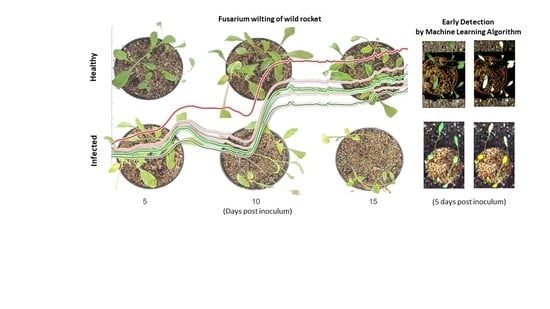
The development of the disease was monitored during a 15-day time-course from inoculations (Figure 1): The time patterns of DI% and DS% showed sub-linear increasing behavior (Figure 2a,b). Survey of infected plants during the time-course indicated that the first symptoms were barely detectable at 5 dpi with slight leaf chlorosis.
Then, the yellowing became progressively severe as the days passed and the diseased plants became stunted with some necrosis on the leaves. However, at intermediate time points that the severity of the disease showed some variability among plants, indicating that the infection was not perfectly synchronized. At the end of the experiment, all infected plants were symptomatic and displayed drastic physiological changes, such as visible growth alterations in the presence of disease-associated symptoms. About 30% out of them were dead, while DI% and DS% reached levels averaging about 100 and 80%, respectively. PCR quantification of FOR genomic DNA was performed to assess the magnification of fungal spread in the vessels and colonization of plant stems from the earliest stages of infection. It was accurately quantified against the standard curve with a linear correlation coefficient (R2) value of 0.9953 (Figure 2c). Consistent with the described phenotypic patterns of the disease, a stepwise increase in fungal DNA was also detected in infected plants over time (Figure 2d). In addition, to verify that the BrightGreen dye detected only a PCR product, samples were subjected to the heat dissociation protocol in the final PCR cycle. Thus, the dissociation curve showed a single peak, demonstrating the presence of only one product in the reaction.
3.3. Plant Reflectance Datasets
Reflectance profiles obtained by means of all pixel-wise spectral data from healthy and infected plants in the spectral range of 400–1000 nm, were displayed for each time point from 5 to 15 dpi (Figure 3a).
During the incubation period of the FOR/wild rocket, the differences between the reflectance levels in infected and healthy samples (Dif. = λF − λC) started to increase, at 5 dpi, in the regions between 520–580 (green) nm and 680–1000 nm (red edge and near infrared). Moving up to 10 dpi, slight differences even in the NIR spectral region (750–1000 nm) began to be consolidated. At 15 dpi, the spectral signature of diseased plants showed dramatic incremental shifts across the analyzed spectrum consistent with the highest DSC levels of disease severity (DSC 3). In this perspective, visualizing the changes in reflectance patterns according to disease severity class, there were no significant differences to show between DSC 0 and DSC 1, while in plants displaying a DSC 2 of disease, substantially increased reflectance in the 400–700 nm range was observed (Figure 3b).
3.4. Temporal Patterns of Hyperspectral Vegetative Indices
Spectral signatures of infected samples during disease progression were first characterized by calculating 54 literature hyperspectral indices (Table S1) reported to be able to describe specific biochemical and/or physiological properties of plants [37]. Then, the most informative VIs, based on their best correlation with disease, were selected by performing stepwise multivariate data analysis. Principal component analysis performed on the differential VIs of Fusarium wilted minus healthy plants, showed a distribution of cases (samples) along the first two components (PC1 and 2) representing, respectively, for 55 and 17.8% of the total variability with one time point (5 to 15 dpi), clustering based along PC1 (Figure 4a,b).
The best VIs candidates for the ability to discriminate between healthy and infected plant status over time are selected based on the highest values of variable correlation with PC1 than a R2 threshold value of 0.90, assuming that this component alone can explain most of the variability in samples attributable to the in vivo experiment disease severity (Figure 4c). Thus, 12 out of 54 vegetation indices were identified showing Pearson’s coefficient greater than 0.90 in direct correlation with DSI (Figure 5). Thus, the best performing vegetation indices were: PRI515, RVI, G, and RGRcn, which are positively correlated with DSI and: NDVI, Red Edge NDVI, OSAVI, HVI, mNDVI705, HNDVI, NDVI 705, and SAVI, which were negatively correlated with DSI. In addition, each of the selected indices was tested alone with a two-way ANOVA to significantly differentiate healthy from infected plants at each time-point. As shown in Figure 6, all selected indices were significant in describing narrow spectral differences between infected and healthy plants at 10 dpi, except mNDVI705, which captured significant differences only at 15 dpi. These 12 selected VIs were subjected to a further restricted PCA that showed the distribution of cases along PC1, explaining almost all the variability contained in the dataset (93.8%), closely related to the DSC level, with a clear separation between clusters of healthy and infected plant in the DSC range between 1.5 and 3 (Figure 7).
However, there was an overlap between infected plants with DSC levels below 1.5 and healthy ones. The high degree of separation of diseased from healthy samples by the selected VIs was also shown by hierarchical clustering, where the highest DSC values corresponded to the highest values (in absolute terms) of each hyperspectral VIs (Figure 8).
3.5. PERMANOVA Results
The PCA was able to identify 26 orthogonal PC axes that explained approximately 95.3% of the total variances and were used to feed into the following analyses. The 100 PERMANOVA tests performed with as many random samples from the complete dataset (including both control and infected plants) found significant differences between groups in only a few cases. PERMANOVA gives only one result on mean distances between all classes considered, whereas we were also interested in pairwise differences between groups. Therefore, we ran the pairwise version of PERMANOVA to test whether the number of significant differences between healthy and highly infected plants was greater than the number of significant differences between healthy and early infected plants. The results showed that, in fact, only 1 simulation out of 100 showed significant differences between DSC class 0 (the healthy plant pixels) and DSC 1 (the early infected), while 2 simulations out of 100 showed significant differences between DSC 0 and DSC 2, and 3 simulations showed significant differences between DSC 0 and DSC 3. In addition, 6 simulations out of 100 produced significant differences between DSC 1 and DSC 2, 3 produced significant differences between DSC 1 and DSC 3, and 6 simulations out of 100 produced significant differences between DSC 2 and DSC 3. With the same pairwise comparisons but taking into account the contribution of the dpi, we found that only 3 simulations out of 100 produced significant differences. When considering the pot identity (POTS), the pairwise PERMANOVA tests showed that only 5 simulations out of 100 produced significant differences between DSC classes. Summary statistics of the 100 pairwise PERMANOVA tests are given in Table S2 in the Supplementary Materials. The single PREMANOVA performed on infected individuals showed only statistically significant differences between DSC (df: 2, F = 1776.13, p << 0.01), dpi (df: 2, F = 19.44, p << 0.01) and POTS (df: 15, F = 102.78, p << 0.01). The pairwise PERMANOVA test performed with infected plants only showed details of significant differences between DSC, dpi, and POTS (see Table 1). The difference between the PERMANOVA results performed on all individuals and on infected plants only shows that pixels on healthy plants negatively affect the ability of the test to discriminate between DSC.
3.6. Machine Learning Models Results and Early Detection
The XGBoost algorithm showed a very high predictive performance on the training dataset. At the pixel level, the accuracy values of the 100 models showed a range of 0.988 and 1 with a mean value of 0.997. The related p-values were all equal to 0, indicating that the abundance of relative classes in the training dataset did not affect the algorithm’s ability to correctly reproduce the observations. Scoring the contribution of the variables to the prediction performance of the 100 training datasets showed that the most important were the spectral bands ranging from the 90 to 94th position (together representing 74% of the models), while the second most important variables included bands 1, those from the 90 to 100th position (excluding the bands in 96th and 97th positions) (together representing 86% of the models) (Figure 9).
With regard to the evaluation of the models by independent observations of individual pixels, and considering the overall accuracy of the indicator predictions, 85 out of 100 test datasets were corrected for the class imbalance problem and all had a prediction accuracy value greater than 0.7 (Figure 10). For healthy pixel class detection, the mean value of detection Precision was 0.78 (ranging from 0.19 to 0.93), the mean Recall was 0.88 (ranging from 0.36 to 1), and the mean F1 Score was 0.82 (ranging from 0.25 to 0.93). With regard to the detection of infected pixels, the average Precision value was 0.73 (ranging from 0.52 to 0.97), the average Recall was 0.57 (ranging from 0.25 to 0.82), and the average F1 Score was 0.63 (ranging from 0.36 to 0.84). Detailed values of the evaluation metrics are given in Table S3 in the Supplementary Materials.
Still considering the indicator prediction strategy, we also employed a model evaluation procedure in which observations at 5, 10, and 15 dpi were used as three separated testing datasets, as previously described in the Material and Methods section. When the testing dataset, including observations at 5 dpi, only are considered, 80 out of 100 testing datasets were corrected for class imbalance. Of these, 39 (49%) had prediction accuracy values greater than 0.7, and 72 (90%) had accuracy values greater than 0.6, demonstrating that very early detection of plant’s disease was a possible but still a difficult task at this stage of disease.
When considering plant pixel datasets at 10 dpi and with an indicator prediction, 62 out of 100 predictions were successfully corrected for class imbalance and 49 of these (79%) showed accuracy values greater than 0.7 (see Figure 10 for a graphical summary of all the results described above). These results are very promising and show that early prediction at 10 dpi is a real feasible task for MLA. After 15 dpi (the mid-stage detection), 95 out of 100 datasets were corrected for class imbalance, and 94 of these (99%) showed accuracy values greater than 0.7. Details on all the evaluation metrics are given in Table S3 of the Supplementary Materials.
When an attempt was made to predict the severity of the disease of the whole individual (i.e., by considering the mean values of the spectral profile of a plant), the prediction results were very encouraging, especially for early detection. In fact, with indicator prediction, 94 out of 100 averaged datasets were corrected for the class imbalance problem. Eighty-six of these showed accuracy values greater than 0.7, with ~92% of cases having good to high prediction success. Regarding the partitioned accuracy for plants with 5 dpi, 41 out of 100 datasets were corrected for class imbalance and all had accuracy values above 0.7. When considering plants with 10 dpi, 46 datasets out of 100 were corrected for class imbalance and, 42 of these (91%) had accuracy values greater than 0.7 (see Figure 10 for a summary of all results described above). After 15 dpi, 89 out of 100 datasets corrected for class imbalance and all of these had accuracy values greater than 0.7.
When we considered the dataset, including all those pixels of plants that were infected but showed no visible symptom of disease (false negatives) after 5 dpi, the 100 XGB models, on average, classified 83% of the pixels as healthy, 17% as DSC 1, and no pixels were classified as DSC 2 or 3. At 10 dpi, the model classified 75% of the false negative pixels as healthy and 25% as DSC 1. No false negatives were visually classified at 15 dpi. Details on all evaluation metrics are given in Table S3 in the Supplementary Materials.
Considering the full models (i.e., models trained with the dataset including all healthy plant pixels, setting apart 8 testing pots, and corrected for class imbalance), the accuracy values for the prediction of the testing dataset at the pixel level was 0.84 (p = 0), the total Precision was 0.95, the Recall was 0.89, and the F1 Score was 0.92. The prediction accuracy of the same dataset but without the correction for class imbalance was 0.896 (p = 0), the total Precision was 0.93, the Recall was 0.99, and the F1 Score was 0.96. Figure 11 shows the predictions of the two models over 4 out of the 8 sampled pots retained to test the models.
The model with correction showed to better classification of infected pixels (sensitivity higher than specificity), while the model without correction performed better in classifying true healthy pixels (specificity higher than sensitivity) (Table 2).
4. Discussion
Hyperspectral sensors capture the reflectance characteristics of an object by measuring a so-called hyperspectral fingerprint in the form of a data cube, which shows the spatial (x, y) and spectral (z) dimensions of the reflectance values per wavelength [38,39]. Many studies have shown that plant reflectance patterns are affected by abiotic stresses, pests, plant pathogens, and/or biological control agents, as well as any other treatments that affect plant physiology, emphasizing the value of hyperspectral imaging sensors in phenotyping, detection, and/or monitoring plant disease [30,40,41,42,43,44,45]. These tools help to highlight spatial variability occurring in the canopy and have shown, in correspondence to previous research, an interesting ability in alert about generalized non-specific changes (symptoms) related to biotic stressors in the basal sap-flow system [46,47].
In the current study, imaging analysis accomplished on FOR-infected plants revealed spectral features associated with disease progression over time, as corroborated by qPCR on interaction DNA in the root collar tract and symptomatic epigeic manifestations displayed by the plants. Hyperspectral fingerprints of infected plant canopies suggested that Fusarium wilt caused a significative reduction in leaf light absorbance compared to the healthy reference in most of the band range increasing over time, probably associated with impairment of photoactive mechanisms related to pigment concentrations, water relations, and cell structure [48]. Fusarium wilt is a dramatic consequence of vessel occlusion due to the plant’s reaction to fungal colonization, which drastically reduces solutes and acropetal water flow affecting color tightness, cell turgor and epigeic tissue activity within a few days, inducing premature leaf senescence and slowing down plant growth [49]. Olivain and Alabouvette [50] documented with microscopy photographs the dynamics of colonization of tomato by a pathogen Fusarium oxysporum f. sp. lycopersici (Saccardo) Snyder & Hansen, which starts from wounds in the roots and leads to vascular infection in the stem just within 7 days from penetration, after the fungus has passed through the plant’s defenses (i.e., biochemical deposits and physical barriers). It is plausible that the endophytic growth of the pathogen in wild rocket plants, which are smaller than tomato, produced detectable distress effects already near the first time point of this study, worsening over time. Indeed, quantification of endophytic fungal DNA revealed the FOR-colonization rate of the wild rocket vascular system, indicating a temporary arrest of fungal spread in the range 5–10 dpi, probably due to the overcoming of plant defenses activated by pathogen/damage-associated molecular patterns [51,52]. As the extent of foliar symptoms is determined by differences in the initiation of infection [53] and the rate of colonization [54], this observed lag phase [55] is a prelude to the observed outbreak of disease at 15 days.
Spectral changes in the early stages of the disease were strongly based on fluctuations and progressive flattening of reflectance levels detected in the absorption regions of chlorophyll (420–470, 490–550, 630–650, and 650–740 nm) and carotenoids (500–533 nm) as a likely consequence of chloroplast destruction and chlorophyll degradation [56,57,58]. The tendency to decrease photosynthetic efficiency and chlorophyll content is the first visible effect of the tracheofusariosis, as also recorded in the “cultivated rocket” Eruca sativa Mill. by Chitarra et al. [59] just before visible plant withering. Under Fusarium wilting stress, the leaf apparatus is a recipient through the xylem of toxins secreted by the pathogen into the vessels (i.e., fusaric acid), which play a crucial role in damaging mesophyll cell membranes and chloroplasts due to the occurrence of oxidative stress [60,61,62], resulting in the suppression of all related photosynthesis processes, the development of leaf chlorosis, and yellowing [63]. While plant physiological responses to water shortage, which in the long run leads to leaf curling, wilting, and the appearance of necrosis, are somewhat more delayed than the abovementioned pigmentation anomalies due to the activation of plant self-protective mechanisms (i.e., stomatal closure, accumulation of proline, abscisic acid, and soluble sugars) according to the study by Sun et al. [64] on cucumber infected by Fusarium oxysporum f. sp. cucumerinum J.H. Owen. Interestingly, these circumstances are also well captured by hyperspectral fingerprinting. Indeed, in advanced stages of wild rocket tracheofusariosis, a stronger increase in leaf reflectance was observed around the near-infrared wavelength range (700–1000 nm), indicating deep changes in leaf health (700–750 nm), cell structure (760–800 nm), biochemical characteristics (800–960 nm), protein (900–920 nm), and water content (960–980 nm) [65,66]. According to the current hyperspectral patterns, with reference to Solanum lycopersicum L./F. oxysporum pathogenesis, Marín Ortiz et al. [67] associated the increase in reflectance levels in the VIS 510–520, 650–670, and 700–750 nm ranges to the lowering of leaf photosynthetic pigments due to the infection, while only a tenuous variation in the 750–1000 nm region was attributed to a marginal disturbance of the water state.
In the current study, 54 different VIs from the literature were applied to the dataset in order to reduce data noise [68], and to help characterize the observed biological phenomena based on reflectance patterns. A total of 12 out of these VIs are highly correlated with the progression of Fusarium wilting (Pearson R2 > 0.9) and belong to the NDVI group (NDVI, HNDVI, mNDVI 705, Red Edge NDVI, NDVI 705), which refers to the nutritional and vegetational status of the canopy [69]; the SAVI group (SAVI and OSAVI), which has been proposed to assess canopy cover and to predict yield [70]; the RGB group (G, HVI, RVI, RGRcn) related to photosynthetic pigments [71,72,73,74]; and, finally, PRI 515 alone, relating to water content [75]. Some of these selected indices have already been reported to be meaningfully correlated with the severity of diseases that cause significant physiological and structural changes in the canopy on different plant systems [30]. For example, NDVI has been applied to monitor the progression of Rhizoctonia solani Kühn in lettuce [76] and the disease severity of Ascochyta blight in chickpea [77]. SAVI was successfully used to estimate in the severity of cotton root rot caused by Phymatotrichopsis omnivora (Duggar) Hennebert [78] and Fusarium Head Blight on wheat [79], respectively. The PRI515 index has been proposed as more robust to identify canopy structural changes [80] and as a pre-visual indicator of water stress [75] and has also been successfully applied in the detection of Fusarium Head Blight in wheat in the early stages of disease [81]. G and RVI have been applied for the assessment of the severity of leaf rust (Puccinia triticina f. sp. tritici Eriks.) and powdery mildew of wheat, respectively [82,83]. The spectral location of these VIs is consistent with the dynamic of pathogenesis discussed above. Indeed, VIs related to changes in leaf pigmentation and/or photosynthesis proved useful to discriminate between diseased and healthy plants in the early stages of plant/pathogen interaction with high significance. On the other hand, the VIs referring to plant status next to the plant withering showed the highest levels of significance in the pairwise comparisons.
The MLA we employed proved to be very powerful in discriminating between healthy and diseased plants at any time and even at the level of a single detection pixel. This makes the very early detection of disease a difficult challenge for classical multivariate tools. The statistical analyses we performed proved that the PC axes of the canopy spectral profiles cannot discriminate between true healthy and diseased plants, mainly due to the very high similarity of the reflectance of healthy and infected plants 5 days earlier. On the other hand, once the true healthy plants were removed from the analyses, significant discrimination between different levels of disease severity was possible. The XGBoost algorithm was used with our cross-pot prediction criterion to test model performance on two sets of pots, for model training and for the performance assessment. Predictions were made at both pixel and canopy levels and showed very high accuracy. MLA detected the occurrence of diseased plants at 5 dpi with good accuracy (>0.7) in 85% of all considered datasets, which were statistically balanced in terms of DSC frequency. These predictions were made at the pixel level, i.e., classifying each individual pixel of a leaf as healthy or infected, according to our scores. When we used the average spectral profile of the plant, the XGBoost algorithm produced a good prediction of early detection in 92% of all datasets that we considered statistically balanced in terms of DSCs distribution. Recently, the algorithm has been used to aid the identification of wild rocket plants affected by powdery mildew based on the spectral response [84].
Based on the accuracy results along different time points after infection, we acknowledge that very early detection (5 dpi) is still difficult to carry out; only 39 out of 100 datasets were correctly classified as healthy or infected. Importantly, only 80 out of 100 datasets were corrected for class imbalance implying that ~50% of them could be correctly classified. MLA has been shown to achieve early disease detection at 10 dpi. In fact, 79% of the datasets corrected for class imbalance showed a prediction accuracy greater than 0.7. Detection of an intermediate stage (15 dpi) was an even easier task as 99% of the balanced testing datasets were correctly classified (see Figure 10 for a graphical summary of these results). Our results showed that a good way to correctly discriminate healthy from infected individuals is to use the mean spectral profile of the canopies (Figure 10). The accuracy of cross-pots prediction is only one strategy we employed to test the ability of MLA in the early detection of wild rocket tracheofusariosis. However, we would like to stress here that any good model training strategy includes collecting as many observations as possible in its pipeline. For this reason, we trained two full models with the full datasets of observations and retained only 8 pots separately for their independent evaluation. The first model was built by resampling the least abundant class observations to reduce class imbalance, while the second model was set up without the correction. The choice to also consider a model without correction was dictated by the condition that leaves of healthy and infected plants may share a rather variable portion of their spectral profiles due to the non-specific symptomatology of tracheofusariosis that becomes more evident in the later stages of infection and the empirical assignment of the relative disease score. Thus, the leaves of an infected plant may still have pixels with a spectral profile typical of a healthy plant and in this case, the model may erroneously include the true spectral profiles of the healthy sectors of true diseased leaves in the variability of infected plants, and thus classify the true healthy plants as infected. In this case, it is important to inform the model of this problem by training it without accounting for class imbalance and then, assigning the healthy spectral profiles shared by healthy and infected plants to the true healthy plants. This procedure should reduce the “specificity” component of the prediction accuracy. This strategy is only valid if the class of healthy plants is the most abundant, as in this study. The results of the two full models showed that our hypothesis on this problem was partly true but shed light on a more complicated phenomenon. Taking into account the comparisons between observations and predictions of the full model with and without correction, as expected, the first one misclassified many healthy pixels as infected, while the model without correction solved this problem. In contrast, the model without correction failed because many infected pixels could be classified as healthy. The predictions produced by the model without correction showed more pixels predicted as healthy (white pixels) on both control and infected plants, while the predictions of the model with correction produced more yellow to red (infected) pixels on control plants as well. This means that the two models helped to overcome some classification problems, but both have the following shortcomings: The model with correction for class imbalance is too sensitive to disease detection and thus to the identification of false positive and the model without correction has a higher type I error rate and may fail to identify early stages of infection. We suggest that considering one of the two models depends closely on the task of crop monitoring. If the aim is disease detection because we suspect that the pathogen may have entered the plants, then the model with correction should be used. On the other hand, if we are sure that the plants are somehow protected from possible infection and we simply want to monitor the crop, then the model without correction could be used.
The ML approach skimmed the most important variables (bands) to image-based prediction of wild rocket Fusarium wilt symptoms over time, show the strongest impact of reflectance data acquired from a few wavelengths in the 660–690 nm range corresponding to the so-called red spectral range, which is involved in plants storing energy through photosynthesis [85,86]. Thus, the reflectance in this narrow region can be used as a valid index of the photosynthesis rate, since it correlates with the efficiency of the photochemical processes taking place in the thylakoid membranes of chloroplasts, which host the photosynthetic pigments organized in the photosystems (PS) I and II [87]. Paired molecules of chlorophyll a absorb at 680 nm in the PSII, and at 700 nm in the PSI [88]. The decrease in the absorbance of red light, therefore, is a sign of a non-effective quantum yield of PSII and PSI [89], which in the initial stage of the wilting progression can be explained by the degradation of chlorophyll a and peroxidation of the thylacoid plasmalemma due to the photoprotective action of ethylene induced by exposure to F. oxysporum toxin, accompanied also by a significant reduction in stomatal conductance [90]. Indeed, this evidence is consistent with the results of previous research concerning chlorophyll-associated VIs that are highly correlated with F. oxysporum disease progression on Physalis peruviana L. [91], and on banana [92]. These results highlighted the importance of capturing hyperspectral information on chlorophyll a transported by PSII in the phospholipidic membrane of thylacoids, to detect early infections of F. oxysporum f. sp. raphani on wild rocket. Finally, it is noticed that bands referable to the red-light range are also present in the formula of many of the VIs selected in this work for the effective early identification of latent infections. Thus, identifying only hyperspectral information that is strictly necessary for crop detection for early disease detection is essential for the application of the spectral approach on a larger scale, such as field uses. Indeed, upscaling possibilities depend on several factors including the simplicity, lightness, and cost-effectiveness of the sensor, which may facilitate, for example, its incorporation into carriers (e.g., light drones, tractors, operating machines) or greenhouses structural supports. This study is designed for the acquisition of top-view hyperspectral images, under conditions, even if controlled, that are very close to the real ones in which wild rocket vegetation grows at the soil line. However, the system needs to be implemented for practical applications, taking into account other limiting factors such as the distribution of plant leaves at different heights and/or stages and bidirectional reflectance distribution function that defines the scattering of the reflected radiance that may require correction [93]. The research conducted here aims to support farmers towards the effective monitoring and management of tracheofusariosis of wild rocket by benefiting from the non-destructive early identification of the plant’s spectral response to pathogenesis. Since fungal infection develops endophytically in a short period of time far before symptoms have become widely visible, the rapidity of intervention with preventive and/or curative measures, is crucial to prevent further spread of the disease and/or to circumscribe and isolate outbreaks, limiting both current and future crop damage (e.g., inoculum accumulation). The optoelectronic sensor system is also potentially scalable, allowing high throughput monitoring of large aboveground areas and mapping of potential outbreaks in a short time, providing information well in advance of traditional visual surveillance. In this perspective, the early identification of diseased plants, such as a kind of invasive alien species, to be treated or eliminated from cultivation can be strategic to improve the results of phytopathological crop management.
5. Conclusions
High-performance VIs that were selected in this work were able to capture spectral changing referring to the progression of Fusarium wilting on wild rocket, proving to be effective in discriminating between different disease stages, and was corroborated by ANOVA tests. Hyperspectral imaging proved to be a powerful and accurate approach to assess the spatio-temporal distribution of spectral fingerprints of diseased and healthy plants, in a perspective of disease early detection. Although powerful classical statistical techniques were not able to detect differences between uninfected plants and less evident symptoms of infection, the XGBoost modeling algorithm proved to have high predictive performance for the early stages of disease detection, even with totally independent testing data, as in the cross-pots prediction evaluation strategy we performed here. Discrimination between healthy and infected pixels was accurate in 85% of our experimental cases, while it was accurate in 86% of the studied datasets when the single plant level was considered. At the individual pixel level, with datasets corrected for class imbalances, the detection of the disease signature at a very early stage of infection (5 dpi) was accurate in 49% of the sampled datasets, while the detection of the disease after 10 days (early detection) was accurate in 79%. The identification of spectral bands referable to the red-light range in the ML algorithm could optimize remote sensing strategies to detect infected plants. Therefore, the ML algorithm can support the early identification of diseased wild rocket plants and/or the assessment of their condition by using spectral markers of the canopy that deviate from the normal plant physiology and inform about the health status.
The application of these technologies can guide disease control strategies and proper crop management by foreseeing disease severity overtime, driving the application of antifungal treatments and, subsequently, lowering the chemical pressure on the specific cropping system and the environment in general.
Supplementary Materials
The following are available online at https://www.mdpi.com/article/10.3390/rs14010084/s1, Table S1: Hyperspectral vegetative indices used in this work, Table S2: Summary statistics of the Pairwise Permutational MANOVA, Table S3: Summary statistics of all the evaluation metrics.
Author Contributions
Conceptualization, C.P.; methodology, C.P. and F.C.; software, validation, formal analysis, investigation, C.P., G.M., N.N. and F.C.; writing—original draft preparation C.P. and F.C.; writing—review and editing C.P., G.M., N.N. and F.C.; supervision C.P. and F.C., project administration, funding acquisition, C.P. All authors have read and agreed to the published version of the manuscript.
Funding
This research was funded by the Italian Ministry of Agriculture, Food, and Forestry Policies (MiPAAF), through the AgriDigit project—sub-project ‘Tecnologie digitali integrate per il rafforzamento sostenibile di produzioni e trasformazioni agroalimentari (AgroFiliere)’ (DM 36503.7305.2018 of 20/12/2018).
Institutional Review Board Statement
Not applicable.
Informed Consent Statement
Not applicable.
Data Availability Statement
Data supporting reported results are available, on request, from the corresponding Authors.
Conflicts of Interest
The authors declare no conflict of interest.
References
- Bonasia, A.; Lazzizera, C.; Elia, A.; Conversa, G. Nutritional, biophysical and physiological characteristics of wild rocket genotypes as affected by soilless cultivation system, salinity level of nutrient solution and growing period. Front. Plant Sci. 2017, 8, 300. [Google Scholar] [CrossRef] [Green Version]
- Caruso, G.; Stoleru, V.; De Pascale, S.; Cozzolino, E.; Pannico, A.; Giordano, M.; Teliban, G.; Cuciniello, A.; Rouphael, Y. Production, leaf quality and antioxidants of perennial wall rocket as affected by crop cycle and mulching type. Agronomy 2019, 9, 194. [Google Scholar] [CrossRef] [Green Version]
- Freshplaza. Il Valore del Settore della Rucola in Italia e’ Stimato in 30–40 Milioni di Euro Solo per L’export 2012. Available online: https://www.freshplaza.it/article/4044942/il-valore-del-settore-della-rucola-in-italia-e-stimato-in-30-40-milioni-di-euro-solo-per-l-export/ (accessed on 12 June 2021).
- Caruso, G.; Parrella, G.; Giorgini, M.; Nicoletti, R. Crop systems, quality and protection of Diplotaxis tenuifolia. Agriculture 2018, 8, 55. [Google Scholar] [CrossRef] [Green Version]
- Nicoletti, R.; Raimo, F.; Miccio, G. Diplotaxis tenuifolia: Biology, production and properties. Eur. J. Plant Sci. Biotechnol. 2007, 1, 36–43. [Google Scholar]
- Li, X.; Zhang, Y.; Ding, C.; Jia, Z.; He, Z.; Zhang, T.; Wang, X. Declined soil suppressiveness to Fusarium oxysporum by rhizosphere microflora of cotton in soil sickness. Biol. Fertil. Soils 2015, 51, 935–946. [Google Scholar] [CrossRef]
- Garibaldi, A.; Gilardi, G.; Gullino, M.L. First of Fusarium oxysporum on Eruca vesicaria and Diplotaxis spp. in Europe. Plant Dis. 2003, 87, 2. [Google Scholar] [CrossRef]
- Garibaldi, A.; Gilardi, G.; Gullino, M.L. Evidence for an expanded host range of Fusarium oxysporum f. sp. raphani. Phytoparasitica 2006, 34, 115–121. [Google Scholar] [CrossRef]
- Catti, A.; Pasquali, M.; Ghiringhelli, D.; Garibaldi, A.; Gullino, M.L. Analysis of vegetative compatibility groups of Fusarium oxysporum from Eruca vesicaria and Diplotaxis tenuifolia. J. Phytopathol. 2007, 155, 61–64. [Google Scholar] [CrossRef]
- Taylor, A.; Barnes, A.; Jackson, A.C.; Clarkson, J.P. First Report of Fusarium oxysporum and Fusarium redolens causing wilting and yellowing of wild rocket (Diplotaxis tenuifolia) in the United Kingdom. Plant Dis. 2019, 103, 6. [Google Scholar] [CrossRef]
- Garibaldi, A.; Gilardi, G.; Pasquali, M.; Kejji, S.; Gullino, M.L. Seed transmission of Fusarium oxysporum of Eruca vesicaria and Diplotaxis muralis. J. Plant Dis. Prot. 2004, 111, 345–350. [Google Scholar]
- Martos, V.; Ahmad, A.; Cartujo, P.; Ordoñez, J. Ensuring agricultural sustainability through remote sensing in the era of agriculture 5.0. Appl. Sci. 2021, 11, 5911. [Google Scholar] [CrossRef]
- Weiss, M.; Jacob, F.; Duveiller, G. Remote sensing for agricultural applications: A meta-review. Remote Sens. Environ. 2020, 236, 111402. [Google Scholar] [CrossRef]
- Zhao, Y.R.; Li, X.; Yu, K.Q.; Cheng, F.; He, Y. Hyperspectral imaging for determining pigment contents in cucumber leaves in response to angular leaf spot disease. Sci. Rep. 2016, 6, 27790. [Google Scholar] [CrossRef]
- Blackburn, G.A. Hyperspectral remote sensing of plant pigments. J. Experiment. Bot. 2007, 58, 855–867. [Google Scholar] [CrossRef] [Green Version]
- Thomas, S.; Kuska, M.T.; Bohnenkamp, D.; Brugger, A.; Alisaac, E.; Wahabzada, M.; Behmann, J.; Mahlein, A.K. Benefits of hyperspectral imaging for plant disease detection and plant protection: A technical perspective. J. Plant Dis. Prot. 2018, 125, 5–20. [Google Scholar] [CrossRef]
- Appeltans, S.; Pieters, J.G.; Mouazen, A.M. Detection of leek white tip disease under field conditions using hyperspectral proximal sensing and supervised machine learning. Comput. Electron. Agric. 2021, 190, 106453. [Google Scholar] [CrossRef]
- Bauriegel, E.; Herppich, W.B. Hyperspectral and chlorophyll fluorescence imaging for early detection of plant diseases, with special reference to Fusarium spec. infections on Wheat. Agriculture 2014, 4, 32–57. [Google Scholar] [CrossRef] [Green Version]
- Zhang, Y.; Lee, W.S.; Li, M.Z.; Zheng, L.H.; Ritenour, M.A. Non-destructive recognition and classification of citrus fruit blemishes based on ant colony optimized spectral information. Postharvest Biol. Technol. 2018, 143, 119–128. [Google Scholar] [CrossRef]
- Tsaftaris, S.A.; Minervini, M.; Scharr, H. Machine learning for plant phenotyping needs image processing. Trends Plant Sci. 2016, 21, 989–991. [Google Scholar] [CrossRef] [Green Version]
- Abdulridha, J.; Batuman, O.; Ampatzidis, Y. UAV-based remote sensing technique to detect citrus canker disease utilizing hyperspectral imaging and machine learning. Remote Sens. 2019, 11, 1373. [Google Scholar] [CrossRef] [Green Version]
- Zhu, H.; Chu, B.; Zhang, C.; Liu, F.; Jiang, L.; He, Y. Hyperspectral imaging for presymptomatic detection of tobacco disease with successive projections algorithm and machine-learning classifiers. Sci. Rep. 2017, 7, 4125. [Google Scholar] [CrossRef] [PubMed] [Green Version]
- Liang, J.; Li, X.; Zhu, P.; Xu, N.; He, Y. Hyperspectral reflectance imaging combined with multivariate analysis for diagnosis of Sclerotinia stem rot on Arabidopsis thaliana leaves. Appl. Sci. 2019, 9, 2092. [Google Scholar] [CrossRef] [Green Version]
- Hornero, A.; Zarco-Tejada, P.J.; Quero, J.L.; North, P.R.J.; Ruiz-Gómez, F.J.; Sánchez-Cuesta, R.; Hernandez-Clemente, R. Modelling hyperspectral- and thermal-based plant traits for the early detection of Phytophthora-induced symptoms in oak decline. Remote Sens. Environ. 2021, 263, 112570. [Google Scholar] [CrossRef]
- Nguyen, C.; Sagan, V.; Maimaitiyiming, M.; Maimaitijiang, M.; Bhadra, S.; Kwasniewski, M.T. Early detection of plant viral disease using hyperspectral imaging and deep learning. Sensors 2021, 21, 742. [Google Scholar] [CrossRef]
- Wei, X.; Johnson, M.A.; Langston, D.B.; Mehl, H.L.; Li, S. Identifying optimal wavelengths as disease signatures using hyperspectral sensor and machine learning. Remote Sens. 2021, 13, 2833. [Google Scholar] [CrossRef]
- Chen, T.; Guestrin, C. XGBoost: A Scalable Tree Boosting System. In Proceedings of the 22nd ACM SIGKDD International Conference on Knowledge Discovery and Data Mining, San Francisco, CA, USA, 13–17 August 2016; pp. 785–794. [Google Scholar] [CrossRef] [Green Version]
- Larkin, R.P.; Honeycutt, C.W. Effects of different 3-year cropping systems on soil microbial communities and Rhizoctonia diseases of potato. Phytopathology 2006, 96, 68–79. [Google Scholar] [CrossRef] [Green Version]
- Chiang, K.S.; Liu, H.I.; Bock, C.H.A. Discussion on disease severity index values. Part I: Warning on inherent errors and suggestions to maximize accuracy. Ann. Appl. Biol. 2017, 171, 139–154. [Google Scholar] [CrossRef]
- Manganiello, G.; Nicastro, N.; Caputo, M.; Zaccardelli, M.; Cardi, T.; Pane, C. Functional hyperspectral imaging by high-related vegetation indices to track the wide-spectrum Trichoderma biocontrol activity against soil-borne diseases of baby-leaf vegetables. Front. Plant Sci. 2021, 12. [Google Scholar] [CrossRef]
- Atoui, A.; El Khoury, A.; Kallassy, M.; Lebrihi, A. Quantification of Fusarium graminearum and Fusarium culmorum by real-time PCR system and zearalenone assessment in maize. Int. J. Food Microbiol. 2012, 15, 59–65. [Google Scholar] [CrossRef] [Green Version]
- Khandekar, S.; Leisner, S. Soluble silicon modulates expression of Arabidopsis thaliana genes involved in copper stress. J. Plant Physiol. 2011, 168, 699–705. [Google Scholar] [CrossRef]
- Hijmans, R.J.; Van Etten, J.; Cheng, J.; Mattiuzzi, M.; Sumner, M.; Greenberg, J.A.; Hiemstra, P.; Hingee, K.; Karney, C.; Mattiuzzi, M.; et al. Package ‘raster’. R Package 2015, 734, 1–94. [Google Scholar]
- Kassambara, A.; Mundt, F. Package ‘Factoextra’. Extract and Visualize the Results of Multivariate Data Analyses 76. 2017. Available online: https://cloud.r-project.org/package=factoextra (accessed on 16 June 2021).
- R Core Team. R: A Language and Environment for Statistical Computing; R Foundation for Statistical Computing: Vienna, Austria, 2021. [Google Scholar]
- Kuhn, M. Building Predictive Models in R Using the caret Package. J. Stat. Softw. 2008, 28, 1–26. [Google Scholar] [CrossRef] [Green Version]
- Xue, J.; Su, B. Significant remote sensing vegetation indices: A review of developments and applications. J. Sens. 2017, 2017, 1353691. [Google Scholar] [CrossRef] [Green Version]
- Thomas, S.; Behmann, J.; Steier, A.; Kraska, T.; Muller, O.; Rascher, U.; Mahlein, A.K. Quantitative assessment of disease severity and rating of barley cultivars based on hyperspectral imaging in a non-invasive, automated phenotyping platform. Plant Methods 2018, 14, 45. [Google Scholar] [CrossRef] [PubMed] [Green Version]
- Jensen, J.R. Remote Sensing of the Environment: An Earth Resource Perspective, 2nd ed.; Pearson Education: London, UK, 2006. [Google Scholar]
- Bravo, C.; Moshou, D.; Oberti, R.; West, J.; McCartney, A.; Bodria, L.; Ramon, H. Foliar disease detection in the field using optical sensor fusion. Agric. Eng. Int. CIGR J. Sci. Res. Dev. 2004, 6, 1–14. [Google Scholar]
- Hillnhütter, C.; Mahlein, A.K.; Sikora, R.A.; Oerke, E.C. Use of imaging spectroscopy to discriminate symptoms caused by Heterodera schachtii and Rhizoctonia solani on sugar beet. Precis. Agric. 2012, 13, 17–32. [Google Scholar] [CrossRef]
- Wahabzada, M.; Kersting, K.; Bauckhage, C.; Römer, C.; Ballvora, A.; Pinto, F.; Rascher, U.; Léon, J.; Plümer, L. Latent Dirichlet Allocation Uncovers Spectral Characteristics of Drought Stressed Plants. In Proceedings of the 28th Conference, Avalon, CA, USA, 15–17 August 2012. [Google Scholar]
- Thomas, S.; Wahabzada, M.; Kuska, M.; Rascher, U.; Mahlein, A.K. Observation of plant–pathogen interaction by simultaneous hyperspectral imaging reflection and transmission measurements. Funct. Plant Biol. 2017, 44, 23–34. [Google Scholar] [CrossRef] [PubMed]
- Kuska, M.; Wahabzada, M.; Leucker, M.; Dehne, H.W.; Kersting, K.; Oerke, E.C.; Steiner, U.; Mahlein, A.K. Hyperspectral phenotyping on the microscopic scale: Towards automated characterization of plant-pathogen interactions. Plant Methods 2015, 11, 28. [Google Scholar] [CrossRef] [Green Version]
- Leucker, M.; Mahlein, A.K.; Steiner, U.; Oerke, E.C. Improvement of lesion phenotyping in Cercospora beticola-sugar beet interaction by hyperspectral imaging. Phytopathology 2016, 1, 1–30. [Google Scholar] [CrossRef] [Green Version]
- Hillnhütter, C.; Mahlein, A.K.; Sikora, R.A.; Oerke, E.C. Remote sensing to detect plant stress induced by Heterodera schachtii and Rhizoctonia solani in sugar beet fields. Field Crops Res. 2011, 122, 70–77. [Google Scholar] [CrossRef]
- Susič, N.; Žibrat, U.; Širca, S.; Strajnar, P.; Razinger, J.; Knapič, M.; Vončina, A.; Urek, G.; Gerič Stare, B. Discrimination between abiotic and biotic drought stress in tomatoes using hyperspectral imaging. Sens. Actuators B Chem. 2018, 273, 842–852. [Google Scholar] [CrossRef] [Green Version]
- Wang, M.; Sun, Y.; Sun, G.; Liu, X.; Zhai, L.; Shen, Q.; Guo, S. Water balance altered in cucumber plants infected with Fusarium oxysporum f. sp. cucumerinum. Sci. Rep. 2015, 5, 7722. [Google Scholar] [CrossRef] [PubMed] [Green Version]
- Pshibytko, N.L.; Zenevich, L.A.; Kabashnikova, L.F. Changes in the photosynthetic apparatus during Fusarium wilt of tomato. Russ. J. Plant Physiol. 2006, 53, 25–31. [Google Scholar] [CrossRef]
- Olivain, C.; Alabouvette, C. Process of tomato root colonization by a pathogenic strain of Fusarium oxysporum f. sp. lycopersici in comparison with a non-pathogenic strain. New Phytol. 1999, 141, 497–510. [Google Scholar] [CrossRef]
- Benhamou, N.; Garand, C. Cytological analysis of defense related mechanisms induced in pea root tissues in response to colonization by nonpathogenic Fusarium oxysporum Fo47. Phytopathology 2001, 91, 730–740. [Google Scholar] [CrossRef] [Green Version]
- Pu, Z.; Ino, Y.; Kimura, Y.; Tago, A.; Shimizu, M.; Natsume, S.; Sano, Y.; Fujimoto, R.; Kaneko, K.; Shea, D.J.; et al. Changes in the proteome of xylem sap in Brassica oleracea in response to Fusarium oxysporum Stress. Front. Plant Sci. 2016, 7, 31. [Google Scholar] [CrossRef] [Green Version]
- Lagopodi, A.L.; Ram, A.F.J.; Lamers, G.E.M.; Punt, P.J.; Van den Hondel, C.A.M.J.J.; Lugtenberg, B.J.J.; Bloemberg, G.V. Novel aspects of tomato root colonization and infection by Fusarium oxysporum f. sp. radicis-lycopersici revealed by confocal laser scanning microscopic analysis using the green fluorescent protein as a marker. Mol. Plant Microbe Interact. 2002, 15, 172–179. [Google Scholar] [CrossRef] [Green Version]
- Gao, H.; Beckman, C.H.; Mueller, W.C. The rate of vascular colonization as a measure of the genotypic interaction between various cultivars of tomato and various formae or races of Fusarium oxysporum. Physiol. Mol. Plant Pat. 1995, 46, 29–43. [Google Scholar] [CrossRef]
- Baayen, R.P.; van der Plas, C.H. Localization ability, latent period and wilting rate in eleven carnation cultivars with partial resistance to Fusarium wilt. Euphytica 1992, 59, 165–174. [Google Scholar] [CrossRef]
- Kang, Z.; Buchenauer, H. Cytology and ultrastructure of the infection of wheat spikes by Fusarium culmorum. Mycol. Res. 2000, 104, 1083–1093. [Google Scholar] [CrossRef]
- Bauriegel, E.; Giebel, A.; Geyer, M.; Schmidt, U.; Herppich, W.B. Early detection of Fusarium infection in wheat using hyper-spectral imaging. Comput. Electron. Agric. 2011, 75, 304–312. [Google Scholar] [CrossRef]
- Muhammed, H.H.; Larsolle, A. Feature vector based analysis of hyperspectral crop reflectance data for discrimination and quantification of fungal disease severity in wheat. Biosyst. Eng. 2003, 86, 125–134. [Google Scholar] [CrossRef]
- Chitarra, W.; Siciliano, I.; Ferrocino, I.; Gullino, M.L.; Garibaldi, A. Effect of elevated atmospheric CO2 and temperature on the disease severity of rocket plants caused by Fusarium Wilt under phytotron conditions. PLoS ONE 2015, 10, e0140769. [Google Scholar] [CrossRef] [Green Version]
- Dong, X.; Xiong, Y.; Ling, N.; Shen, Q.; Guo, S. Fusaric acid accelerates the senescence of leaf in banana when infected by Fusarium. World J. Microbiol. Biotechnol. 2014, 30, 1399–1408. [Google Scholar] [CrossRef]
- Wang, M.; Ling, N.; Dong, X.; Liu, X.; Shen, Q.; Guo, S. Effect of fusaric acid on the leaf physiology of cucumber seedlings. Eur. J. Plant. Pathol. 2014, 138, 103–112. [Google Scholar] [CrossRef]
- Mendoza-Vargas, L.A.; Villamarín-Romero, W.P.; Cotrino-Tierradentro, A.S.; Ramírez-Gil, J.G.; Chávez-Arias, C.C.; Restrepo-Díaz, H.; Gómez-Caro, S. Physiological response of cape gooseberry plants to Fusarium oxysporum f. sp. physali, fusaric acid, and water deficit in a hydrophonic system. Front. Plant Sci. 2021, 12, 702842. [Google Scholar] [CrossRef]
- Singh, V.K.; Singh, H.B.; Upadhyay, R.S. Role of fusaric acid in the development of ‘Fusarium wilt’ symptoms in tomato: Physiological, biochemical and proteomic perspectives. Plant Physiol. Biochem. 2017, 118, 320–332. [Google Scholar] [CrossRef]
- Sun, Y.; Wang, M.; Li, Y.; Gu, Z.; Ling, N.; Shen, Q.; Guo, S. Wilted cucumber plants infected by Fusarium oxysporum f. sp. cucumerinum do not suffer from water shortage. Ann. Bot. 2017, 120, 427–436. [Google Scholar] [CrossRef]
- Ceccato, P.; Gobron, N.; Flasse, S.; Pinty, B.; Tarantola, S. Designing a spectral index to estimate vegetation water content from remote sensing data: Part I: Theoretical approach. Remote Sens. Environ. 2002, 82, 188–197. [Google Scholar] [CrossRef]
- Zarco-Tejada, P.J.; Pushnik, J.C.; Dobrowski, S. Steady-state chlorophyll a fluorescence detection from canopy derivative reflectance and double-peak red-edge effects. Remote Sens. Environ. 2003, 84, 283–294. [Google Scholar] [CrossRef]
- Marín Ortiz, J.C.; Hoyos Carvajal, L.M.; Botero Fernandez, V. Detection of significant wavelengths for identifying and classifying during the incubation period and water stress in plants using reflectance spectroscopy. J. Plant Prot. Res. 2019, 59, 244–254. [Google Scholar] [CrossRef]
- Carter, G.A.; Miller, R.L. Early detection of plant stress by digital imaging within narrow stress-sensitive wavebands. Remote Sens. Environ. 1994, 50, 295–302. [Google Scholar] [CrossRef]
- Zhou, G.; Yin, X. Assessing nitrogen nutritional status, biomass and yield of cotton with NDVI, SPAD and petiole sap nitrate concentration. Exp. Agric. 2018, 54, 531–548. [Google Scholar] [CrossRef]
- Steven, M.D.; Jaggard, K.W. Advances in Crop Monitoring by Remote Sensing. In Advances in Environmental Remote Sensing; Danson, F.M., Plummer, S.E., Eds.; John and Wiley and Sons: Hoboken, NJ, USA, 1995; pp. 143–156. [Google Scholar]
- Smith, R.C.G.; Adams, J.; Stephens, D.J.; Hick, P.T. Forecasting wheat yield in a Mediterranean-type environment from the NOAA satellite. Aus. J. Agric. Res. 1995, 46, 113. [Google Scholar] [CrossRef]
- Gitelson, A.A.; Merzlyak, M.N.; Lichtenthaler, H.K. Detection of red edge position and chlorophyll content by reflectance measurements near 700 nm. J. Plant Physiol. 1996, 148, 501–508. [Google Scholar] [CrossRef]
- Tilley, D.R.; Ahmed, M.; Son, J.H.; Badrinarayanan, H. Hyperspectral reflectance of emergent macrophytes as an indicator of water column ammonia in an oligohaline, subtropical marsh. Ecol. Eng. 2003, 21, 153–163. [Google Scholar] [CrossRef]
- Steddom, K.; Heidel, G.; Jones, D.; Rush, C.M. Remote detection of rhizomania in sugar beets. Phytopathology 2003, 93, 720–726. [Google Scholar] [CrossRef] [Green Version]
- Stagakis, S.; González-Dugo, V.; Cid, P.; Guillén-Climent, M.L.; Zarco-Tejada, P.J. Monitoring water stress and fruit quality in an orange orchard under regulated deficit irrigation using narrow-band structural and physiological remote sensing indices. ISPRS J. Photogramm. Remote Sens. 2012, 71, 47–61. [Google Scholar] [CrossRef] [Green Version]
- Sandmann, M.; Grosch, R.; Graefe, J. The use of features from fluorescence, thermography, and NDVI imaging to detect biotic stress in lettuce. Plant Dis. 2018, 102, 1101–1107. [Google Scholar] [CrossRef] [Green Version]
- Zhang, C.; Chen, W.; Sankaran, S. High-throughput field phenotyping of Ascochyta blight disease severity in chickpea. Crop Prot. 2019, 125, 104885. [Google Scholar] [CrossRef]
- Zhao, H.; Yang, C.; Guo, W.; Zhang, L.; Zhang, D. Automatic estimation of crop disease severity levels based on vegetation index normalization. Remote Sens. 2020, 12, 1930. [Google Scholar] [CrossRef]
- Liu, L.; Dong, Y.; Huang, W.; Du, X.; Ma, H. Monitoring wheat Fusarium head blight using unmanned aerial vehicle hyperspectral imagery. Remote Sens. 2020, 12, 3811. [Google Scholar] [CrossRef]
- Hernández-Clemente, R.; Navarro-Cerrillo, R.M.; Suárez, L.; Morales, F.; Zarco-Tejada, P.J. Assessing structural effects on PRI for stress detection in conifer forests. Remote Sens. Environ. 2011, 115, 2360–2375. [Google Scholar] [CrossRef]
- Mahlein, A.K.; Alisaac, E.; Al Masri, A.; Behmann, J.; Dehne, H.W.; Oerke, E.C. Comparison and combination of thermal, fluorescence, and hyperspectral imaging for monitoring Fusarium head blight of wheat on spikelet scale. Sensors 2019, 19, 2281. [Google Scholar] [CrossRef] [Green Version]
- Bhandari, M.; Ibrahim, A.M.; Xue, Q.; Jung, J.; Chang, A.; Rudd, J.C.; Landivar, J. Assessing winter wheat foliage disease severity using aerial imagery acquired from small unmanned aerial vehicle (UAV). Comput. Electron. Agric. 2020, 176, 105665. [Google Scholar] [CrossRef]
- He, L.; Qi, S.L.; Duan, J.Z.; Guo, T.C.; Feng, W.; He, D.X. Monitoring of wheat powdery mildew disease severity using multiangle hyperspectral remote sensing. Trans. Geosci. Remote Sens. 2020, 59, 979–990. [Google Scholar] [CrossRef]
- Pane, C.; Manganiello, G.; Nicastro, N.; Cardi, T.; Carotenuto, F. Powdery mildew caused by Erysiphe cruciferarum on wild rocket (Diplotaxis tenuifolia): Hyperspectral imaging and machine learning modeling for non-destructive disease detection. Agriculture 2021, 11, 337. [Google Scholar] [CrossRef]
- Curran, P.J.; Dungan, J.L.; Gholz, H.L. Exploring the relationship between reflectance red edge and chlorophyll content in slash pine. Tree Physiol. 1990, 7, 33–48. [Google Scholar] [CrossRef]
- Liu, J.; van Iersel, M.W. Photosynthetic physiology of blue, green, and red light: Light intensity effects and underlying mechanisms. Front. Plant Sci. 2021, 12, 619987. [Google Scholar] [CrossRef]
- Lichtenthaler, H.K.; Gitelson, A.; Lang, M. Non-destructive determination of chlorophyll content of leaves of a green and an aurea mutant of tobacco by reflectance measurements. J. Plant Physiol. 1996, 148, 483–493. [Google Scholar] [CrossRef]
- Heber, U.; Shuvalov, V.A. Photochemical reactions of chlorophyll in dehydrated Photosystem II: Two chlorophyll forms (680 and 700 nm). Photosynth. Res. 2005, 84, 85–91. [Google Scholar] [CrossRef] [PubMed]
- Liu, C.; Guo, J.; Cui, Y.; Lü, T.; Zhang, X.; Shi, G. Effects of cadmium and salicylic acid on growth, spectral reflectance and photosynthesis of castor bean seedlings. Plant Soil 2011, 344, 131–141. [Google Scholar] [CrossRef]
- Iqbal, N.; Czékus, Z.; Ördög, A.; Poór, P. Ethylene-dependent effects of fusaric acid on the photosynthetic activity of tomato plants. Photosynthetica 2021, 59, 337–348. [Google Scholar] [CrossRef]
- Giraldo-Betancourt, C.; Velandia-Sánchez, E.A.; Fischer, G.; Gómez-Caro, S.; Martínez, L.J. Hyperspectral response of cape gooseberry (Physalis peruviana L.) plants inoculated with Fusarium oxysporum f. sp. physali for vascular wilt detection. Rev. Colomb. Cienc. Hortíc. 2020, 14, 301–313. [Google Scholar] [CrossRef]
- Ye, H.; Huang, W.; Huang, S.; Cui, B.; Dong, Y.; Guo, A.; Ren, Y.; Jin, Y. Recognition of Banana Fusarium Wilt based on UAV remote sensing. Remote Sens. 2020, 12, 938. [Google Scholar] [CrossRef] [Green Version]
- Yang, Q.; Liu, X.; Wu, W. A Hyperspectral Bidirectional Reflectance Model for Land Surface. Sensors 2020, 20, 4456. [Google Scholar] [CrossRef]
Figure 1.
Photographs of healthy versus FOR-infected potted plants during the experimental time course at 5, 10, and 15 dpi to follow the progression of Fusarium wilting.
Figure 1.
Photographs of healthy versus FOR-infected potted plants during the experimental time course at 5, 10, and 15 dpi to follow the progression of Fusarium wilting.

Figure 2.
Disease incidence (panel (a)) and disease severity (panel (b)) percentages assessed on FOR-infected wild rocket (red line) compared to healthy control (blue line). Standard curve for qPCR quantification of FOR genomic DNA from pure culture against cycle threshold (CT) values (panel (c)). Quantification by qPCR of fungal DNA expressed as picograms (pg) of fungal DNA per nanogram (ng) of the main root and collar DNA (panel (d)). Values with different lowercase letters (a–c) are significantly different (p-value ≤ 0.05) according to ANOVA and Bonferroni correction test for multiple comparisons.

Figure 3.
Hyperspectral reflectance signatures of wild rocket under progression of Fusarium wilting. Comparison of spectral curves of healthy© and FOR-infected (F) plants at 5, 10, and 15 dpi by using color gradients light to dark green and red, respectively (panel (a)). Means of hyperspectral reflectance averages rearranged per level of disease severity class: Healthy, level 0 (DSC 0, green); mild stunting, level 1 (DSC 1, yellow); severe stunting and yellowing, level 2 (DSC 2, orange); and necrosis/dead plants, level 3 (DSC 3, red) (panel (b)).

Figure 4.
Principal component analysis biplot for Fusarium (F)-infected wild rocket plants (n = 90) examined at 5, 10, and 15 dpi in each replicate (1–5) per pot (A–F) (cases, panel (a)) for differential values (infected − healthy) of 54 literature vegetation indices (variables, on panel (b)) according to principal component 1 (PC1) and 2 (PC2) explaining 55.0 and 17.8% of the total variance, respectively. The colors in panel A are related to the observed disease severity classes while in panel b are linked to the contributions (contrib) of each VI to the definition of the principal dimensions. Coefficients of variable correlation with the two principal components are showed in panel (c).

Figure 5.
Pearson’s correlation of the hyperspectral vegetation indices highly correlated (p-value ≤ 0.05 and R2 > 0.9) with disease severity classes (DSC) exhibited by wild rocket infected with F. oxysporum f. sp. raphani.
Figure 5.
Pearson’s correlation of the hyperspectral vegetation indices highly correlated (p-value ≤ 0.05 and R2 > 0.9) with disease severity classes (DSC) exhibited by wild rocket infected with F. oxysporum f. sp. raphani.

Figure 6.
Average of the selected literature hyperspectral vegetation indices calculated on the canopy reflectance data from FOR-infected (F, red) and control healthy (C, dark blue) wild rocket plants at 5, 10, and 15 dpi. Bars with different lowercase letters are significantly different (p-value ≤ 0.05) and asterisks indicate the significance level (* p-value ≤ 0.05; ** p-value ≤ 0.01; *** p-value ≤ 0.001; **** p-value ≤ 0.0001) of the pairwise comparisons between indices of FOR-infected and control healthy plants. Analyses were conducted applying ANOVA and Bonferroni correction test for multiple comparisons.

Figure 7.
Principal component analysis biplot for infected (F, n = 18) and healthy control (C, n = 18) wild rocket pots examined at 5, 10, and 15 dpi (cases) for the 12 selected vegetation indices (variables). Unit variance scaling is applied to the rows; SVD with imputation is used to calculate principal components. X and Y axis show principal component 1 and principal component 2, explaining 93.8% and 2.4% of the total variance, respectively. Color grouping was performed by considering the disease severity classes (DSC) in the range 0 = healthy to 3 = highly infected. The prediction ellipses are such that with probability 0.95, a new observation from the same group will fall within the ellipse.

Figure 8.
Heatmap obtained by hierarchical clustering of the 12 selected vegetation indices in relation to DSC. The analysis was conducted on infected (F, n = 18) and healthy (C, n = 18) wild rocket pots at 5, 10, and 15 dpi. DSC and VIs values represented following color scales A and B, respectively. Indices values (rows) were centered, and a unit variance scale was applied. The different observations (columns) were clustered using maximum distance and Ward linkage.

Figure 9.
Frequency distribution of the most (violet) and second most (green) important variables in the ML models for the 100 iterations of the cross-pots predictions. The x-axis of the plot ends at 104 since this was the maximum spectral band sampled as the two most important predictor variables in the 100 iterations.

Figure 10.
Bar plot showing the frequency of overall and partial accuracy statistics for the 100 resampled testing datasets. Each bar represents the total of the 100 predictions on testing pots (the height from 0 of the violet bar). From the left, the first 4 bars show the prediction results at the pixel level, while the last bar shows the same results but at the plant level. The height from 0 of the blue bars indicates the part of the predictions that have a high accuracy (>0.7). The height of the yellow bars indicates the number of only predictions made on datasets that showed the correction for class imbalance and gave accuracy values greater than 0.7. The height of the light green and orange bars are for special cases: The light green bar indicates that all datasets that were corrected for class imbalance showed high accuracy, while the orange bar indicates that all datasets that showed high accuracy was also corrected for class imbalance.

Figure 11.
Graphical results of full model predictions on independent datasets. The rows of the plots in the figure represent, from the top, the pots of healthy and infected plants at 5 (very early detection), 10 (early detection), and 15 (mid-stage detection) dpi. The columns of the images represent, from the left side, the original image of each pot, the prediction by the model correcting for class imbalance and the prediction produced by the models not correcting for class imbalance. The legend to the right of each prediction indicates the color of each disease stage: White for pixels classified as healthy, yellow for pixels classified as DSC 1, and orange and red indicating as DSC 2 and 3 levels, respectively.


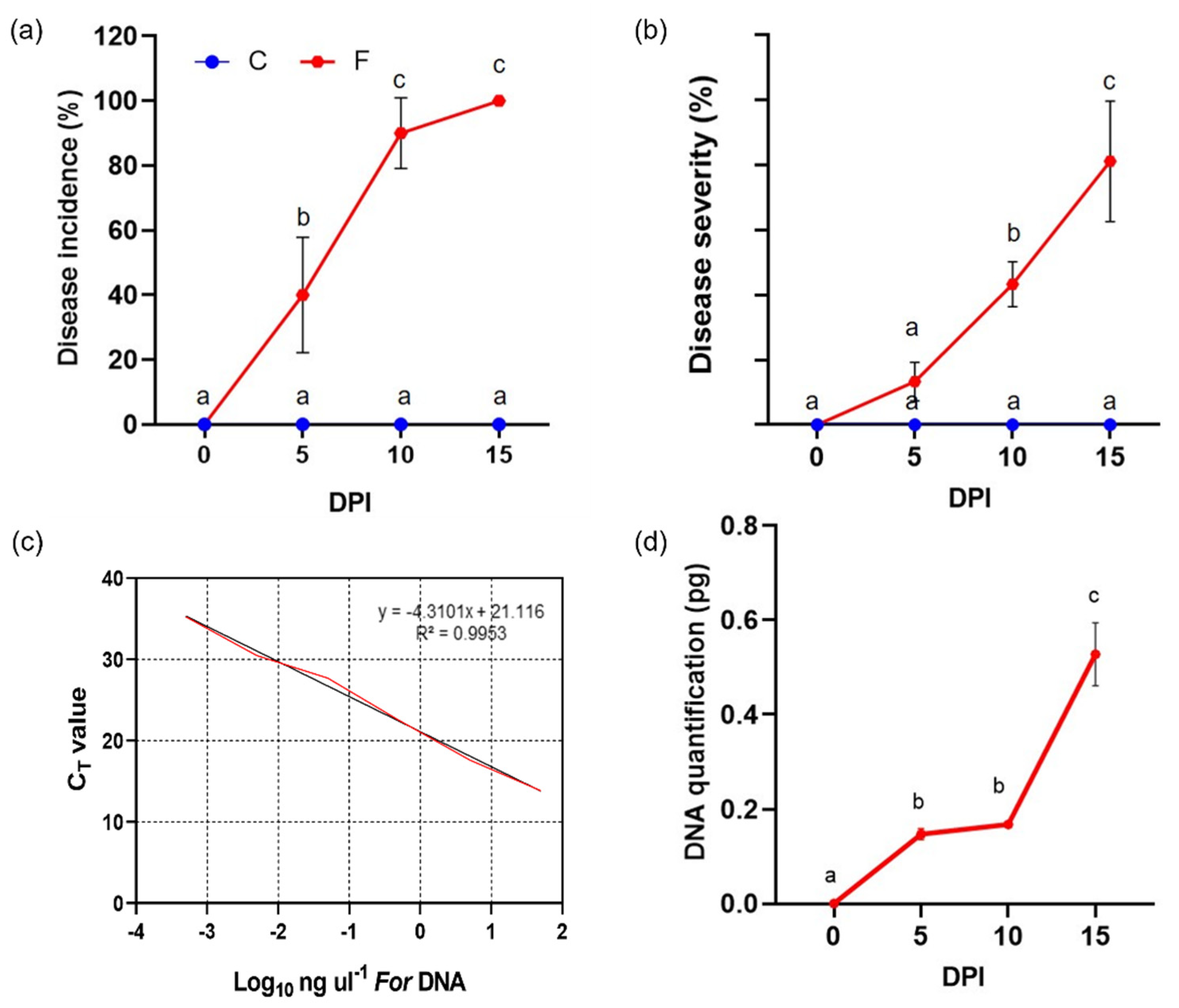
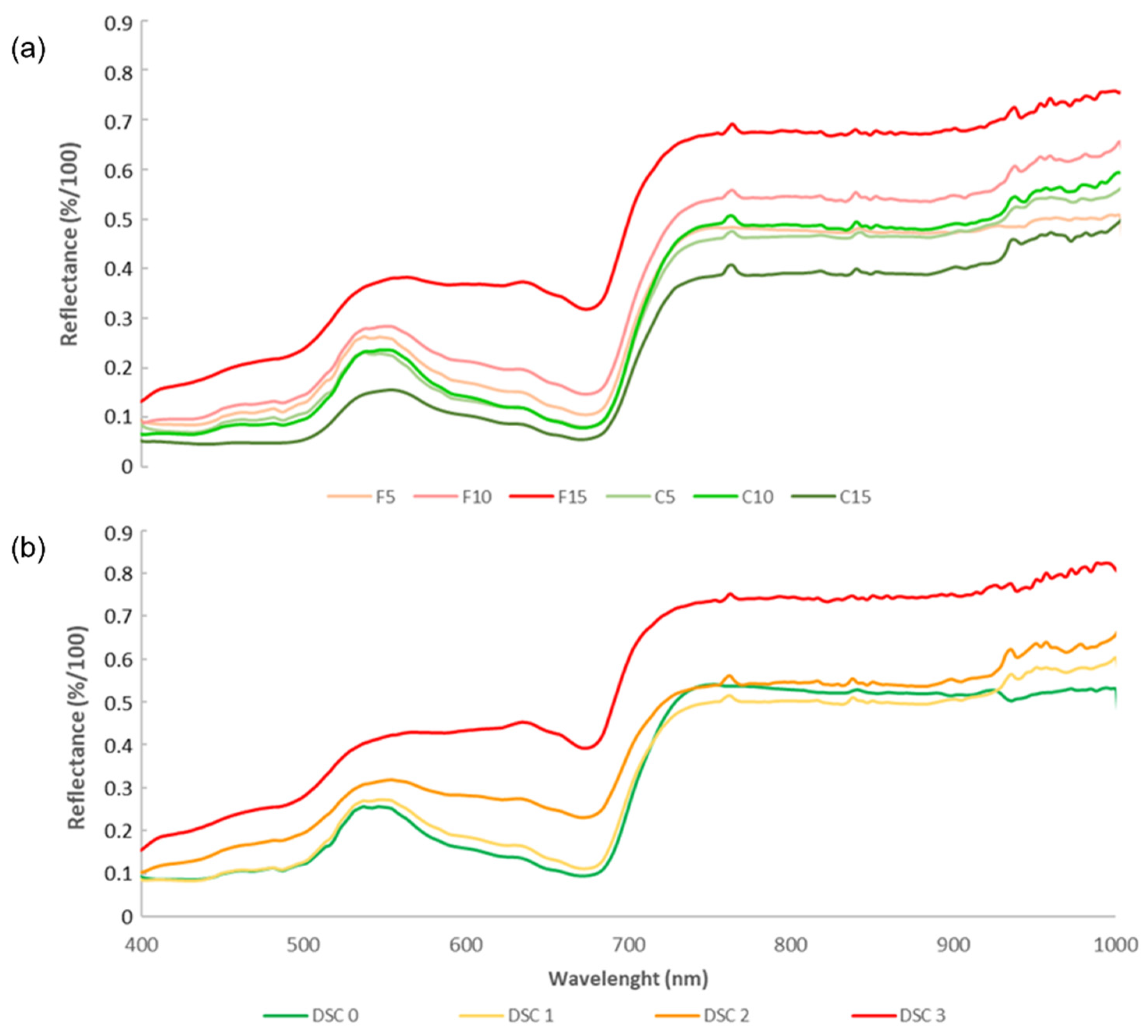
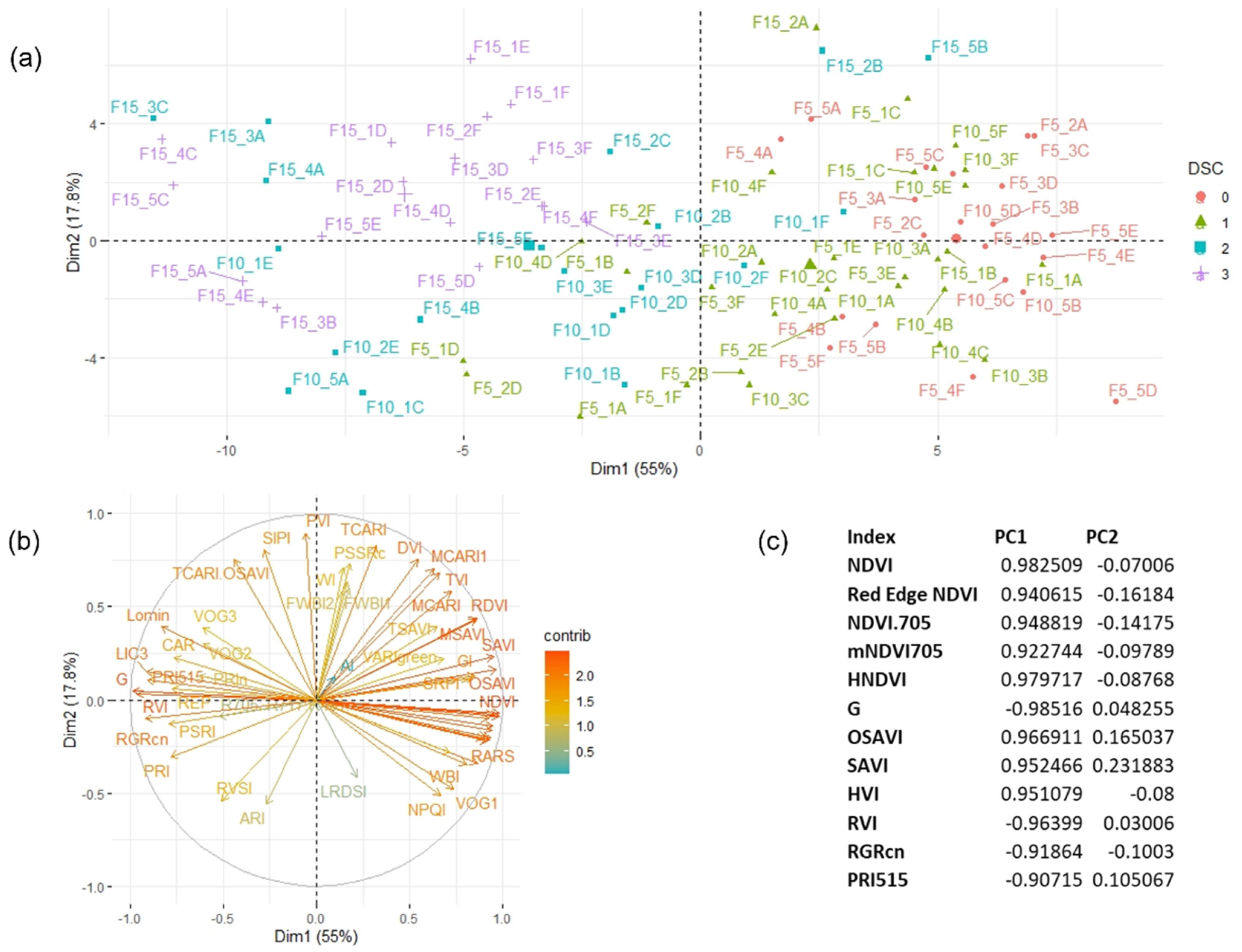
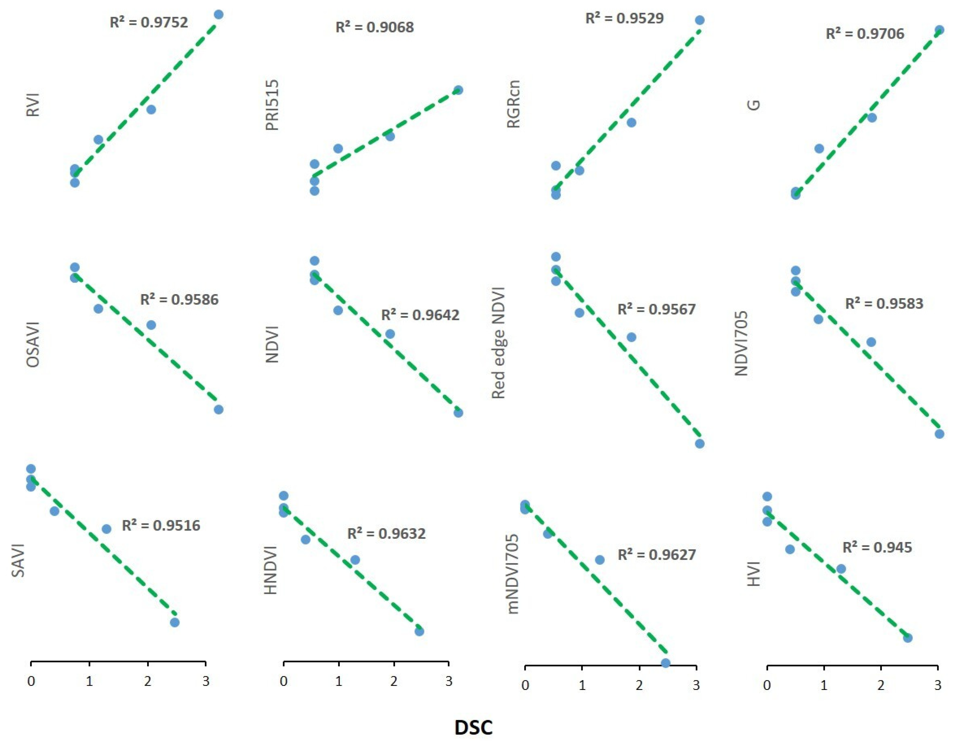
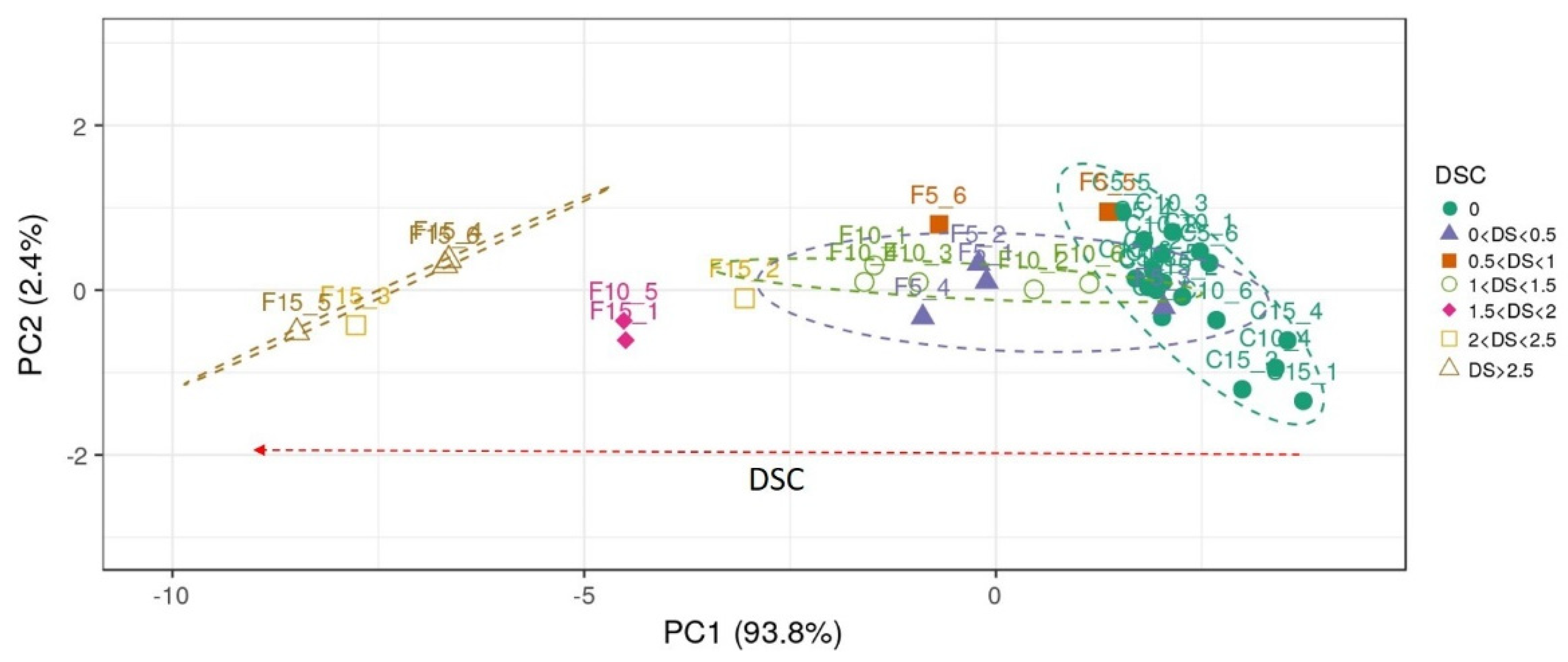
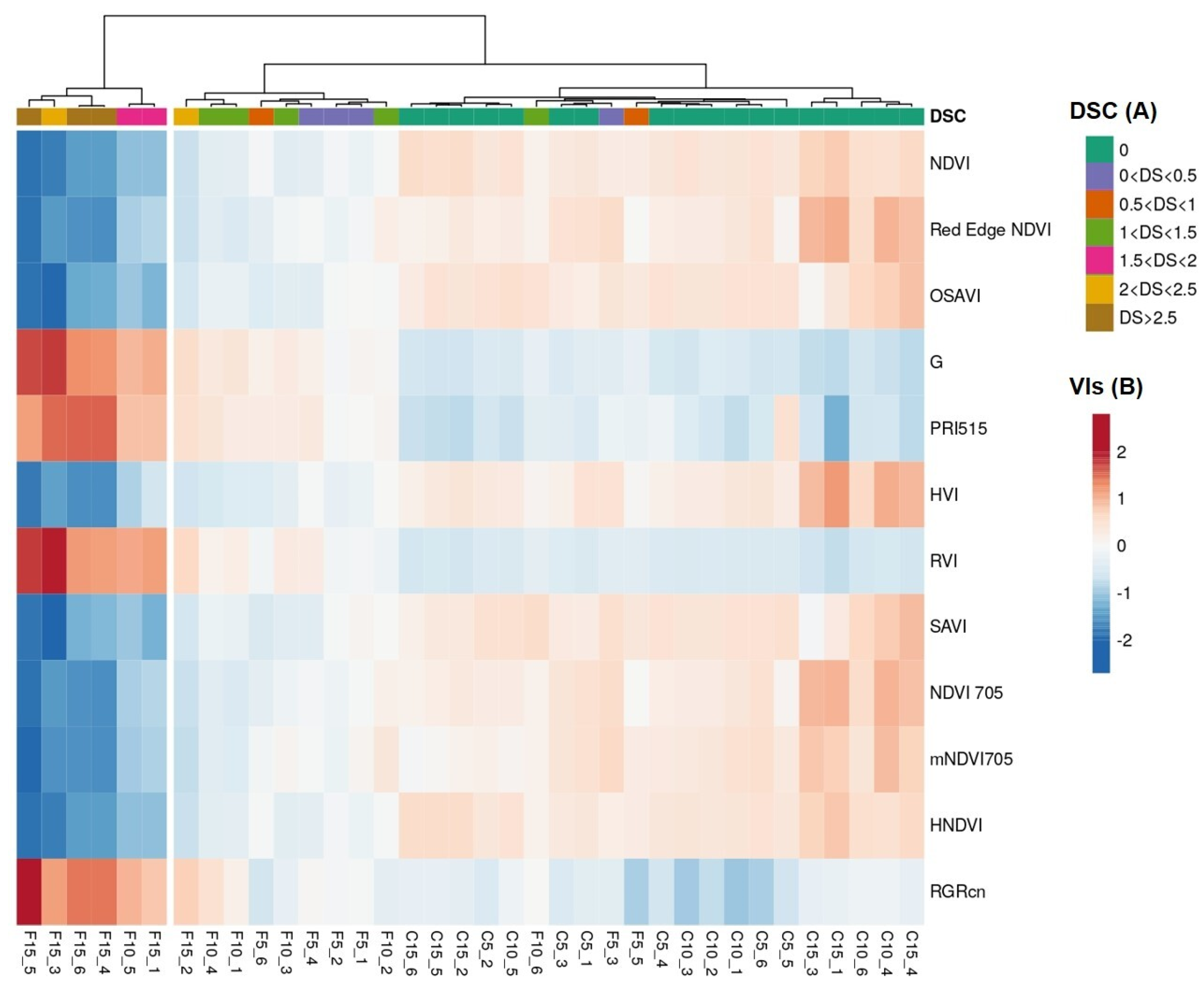
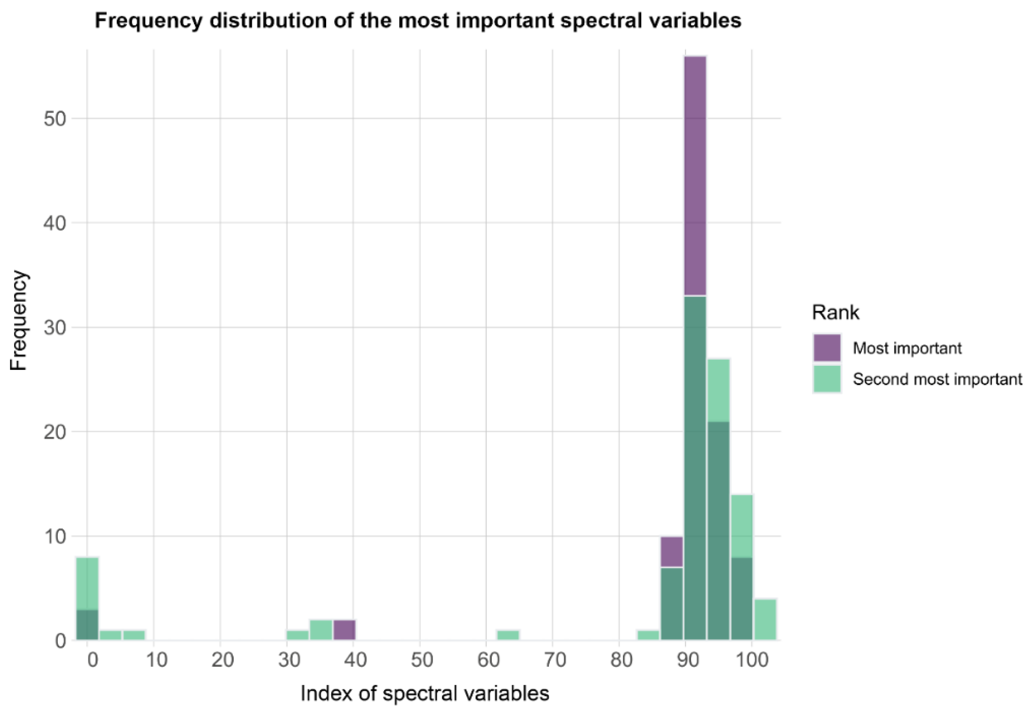
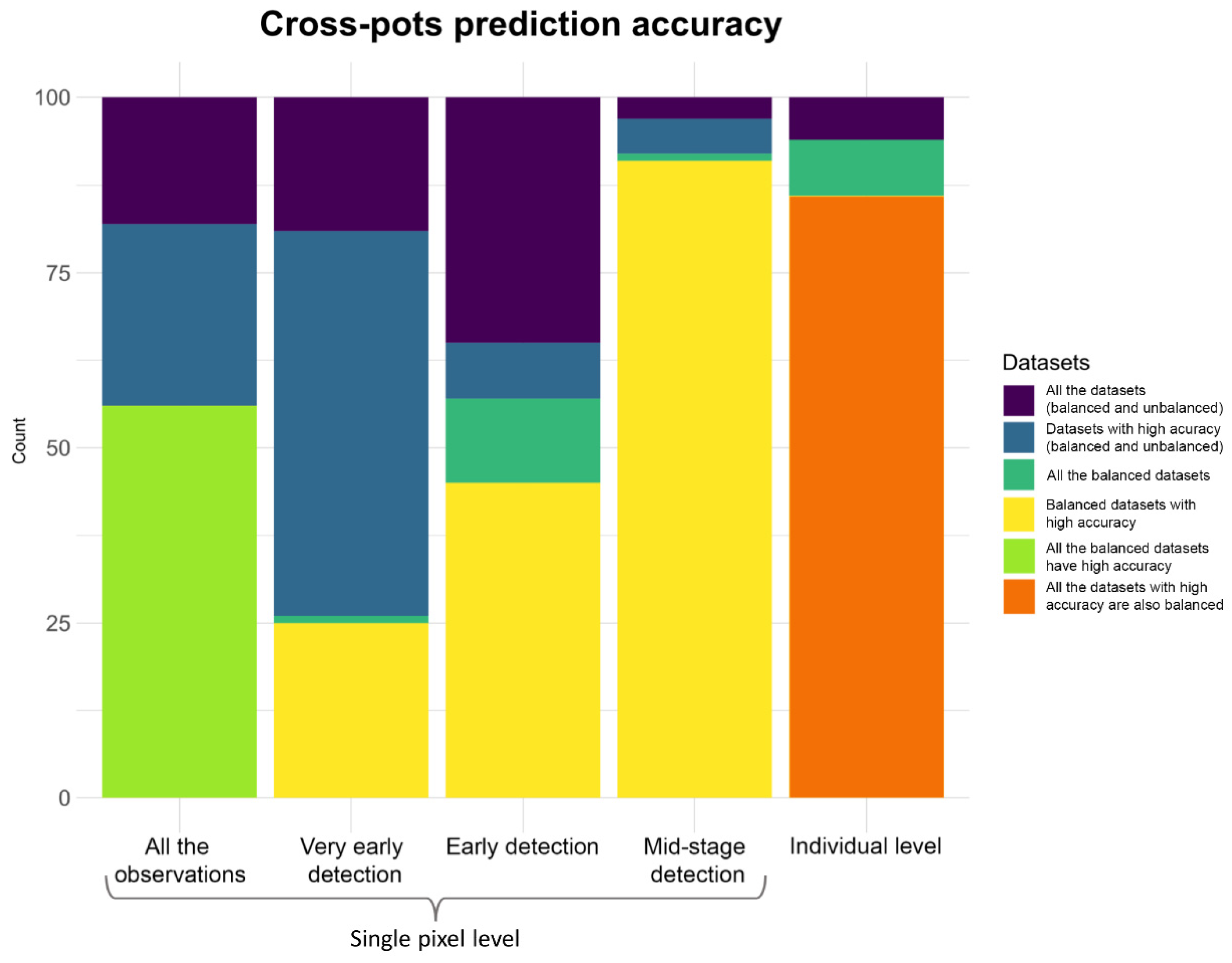
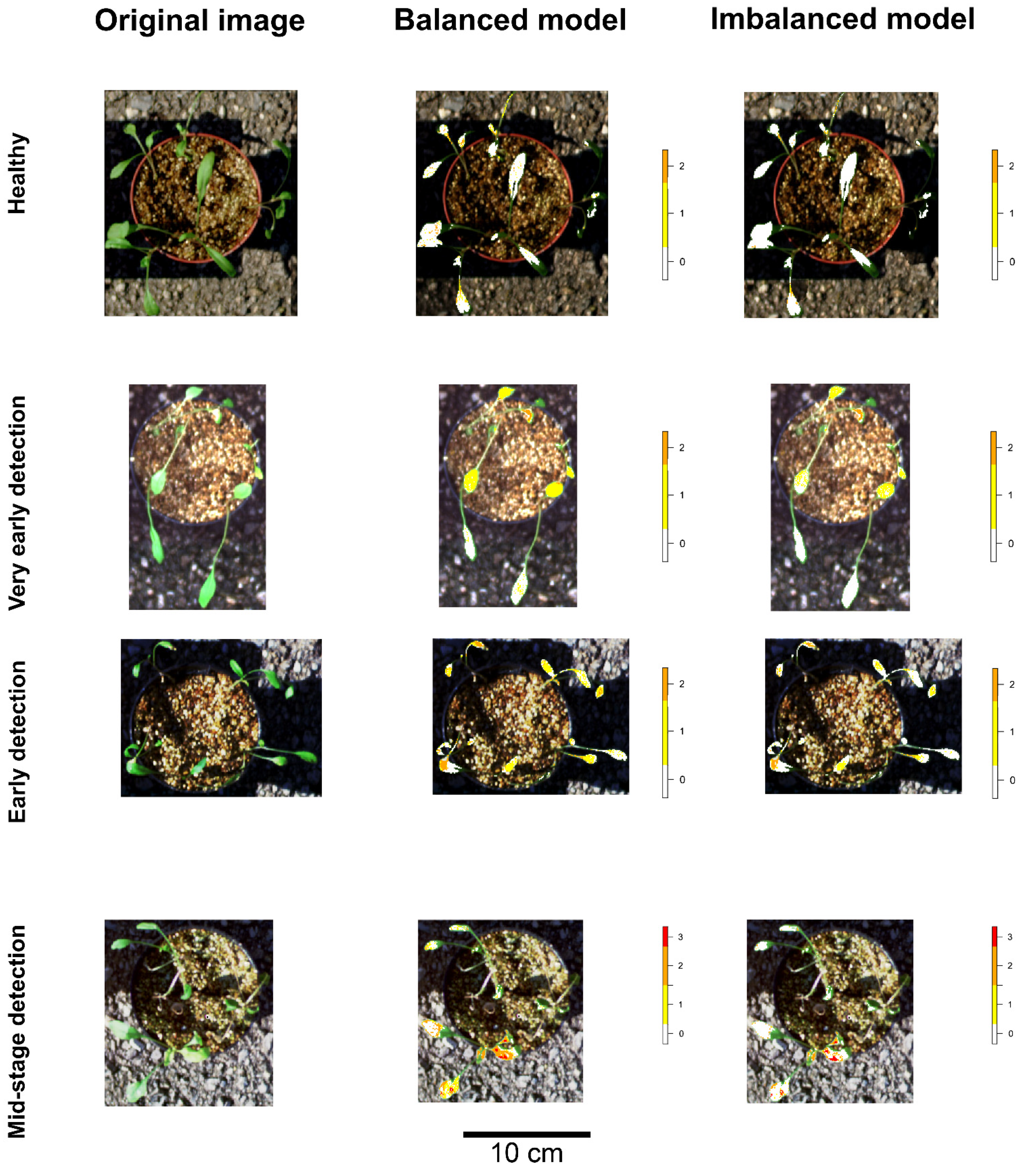
Table 1.
Results of pairwise Permutational MANOVA applied only to infected plants. DSC: Disease severity classes; dpi: Days post infection; and POTS: Pots identification number.
Table 1.
Results of pairwise Permutational MANOVA applied only to infected plants. DSC: Disease severity classes; dpi: Days post infection; and POTS: Pots identification number.
| DSC 1 vs. DSC 2 | |||||
| Df | Sum of Sqs | R2 | F | Pr (>F) | |
| DSC | 1 | 159.8 | 0.02076 | 98.91 | 0.001 |
| dpi | 2 | 69.7 | 0.00905 | 21.57 | 0.001 |
| POTS | 13 | 2170.9 | 0.2819 | 103.33 | 0.001 |
| Residual | 3280 | 5300.6 | 0.6883 | ||
| Total | 3296 | 7701.1 | 1 | ||
| DSC 1 vs. DSC 3 | |||||
| Df | Sum of Sqs | R2 | F | Pr (>F) | |
| DSC | 1 | 6054.3 | 0.43793 | 4308.88 | 0.001 |
| dpi | 2 | 584.1 | 0.04225 | 207.85 | 0.001 |
| POTS | 15 | 2041 | 0.14763 | 96.84 | 0.001 |
| Residual | 3662 | 5145.4 | 0.37219 | ||
| Total | 3680 | 13824.8 | 1 | ||
| DSC 2 vs. DSC 3 | |||||
| Df | Sum of Sqs | R2 | F | Pr (>F) | |
| DSC | 1 | 2958.5 | 0.28265 | 1331.24 | 0.001 |
| dpi | 1 | 343.8 | 0.03285 | 154.72 | 0.001 |
| POTS | 10 | 1348.8 | 0.12886 | 60.69 | 0.001 |
| Residual | 2617 | 5816 | 0.55564 | ||
| Total | 2629 | 10467.3 | 1 | ||
Table 2.
Observations vs. predictions of the full models (with and without correction for class imbalance) on the pot images of the testing datasets. On the left, observations and associated predictions produced by the full model accounting for class imbalance. On the right, observations and predictions produced by the full model not accounting for class imbalance.
| Model with Correction for Class Imbalance | Model without Correction for Class Imbalance | ||||||||||
|---|---|---|---|---|---|---|---|---|---|---|---|
| Observations | Observations | ||||||||||
| Predictions | d0 | d1 | d2 | d3 | Predictions | d0 | d1 | d2 | d3 | ||
| d0 | 6864 | 276 | 43 | 14 | d0 | 7620 | 416 | 122 | 14 | ||
| d1 | 673 | 157 | 81 | 0 | d1 | 68 | 20 | 47 | 7 | ||
| d2 | 158 | 105 | 228 | 182 | d2 | 7 | 102 | 181 | 202 | ||
| d3 | 0 | 0 | 9 | 756 | d3 | 0 | 0 | 11 | 729 | ||
Publisher’s Note: MDPI stays neutral with regard to jurisdictional claims in published maps and institutional affiliations. |
© 2021 by the authors. Licensee MDPI, Basel, Switzerland. This article is an open access article distributed under the terms and conditions of the Creative Commons Attribution (CC BY) license (https://creativecommons.org/licenses/by/4.0/).
Share and Cite
MDPI and ACS Style
Pane, C.; Manganiello, G.; Nicastro, N.; Carotenuto, F. Early Detection of Wild Rocket Tracheofusariosis Using Hyperspectral Image-Based Machine Learning. Remote Sens. 2022, 14, 84. https://doi.org/10.3390/rs14010084
AMA Style
Pane C, Manganiello G, Nicastro N, Carotenuto F. Early Detection of Wild Rocket Tracheofusariosis Using Hyperspectral Image-Based Machine Learning. Remote Sensing. 2022; 14(1):84. https://doi.org/10.3390/rs14010084
Chicago/Turabian StylePane, Catello, Gelsomina Manganiello, Nicola Nicastro, and Francesco Carotenuto. 2022. "Early Detection of Wild Rocket Tracheofusariosis Using Hyperspectral Image-Based Machine Learning" Remote Sensing 14, no. 1: 84. https://doi.org/10.3390/rs14010084
Note that from the first issue of 2016, this journal uses article numbers instead of page numbers. See further details here.