
Large-Scale, Multiple Level-of-Detail Change Detection from Remote Sensing Imagery Using Deep Visual Feature Clustering


Department of Electrical Engineering and Computer Science, University of Missouri, Columbia, MO 65201, USA
*
Author to whom correspondence should be addressed.
Remote Sens. 2021, 13(9), 1661; https://doi.org/10.3390/rs13091661
Submission received: 31 March 2021
/
Revised: 21 April 2021
/
Accepted: 22 April 2021
/
Published: 24 April 2021
(This article belongs to the Special Issue Synergy of Remote Sensing and Deep Learning for Mineral Resources and Environment)
Abstract
:In the era of big data, where massive amounts of remotely sensed imagery can be obtained from various satellites accompanied by the rapid change in the surface of the Earth, new techniques for large-scale change detection are necessary to facilitate timely and effective human understanding of natural and human-made phenomena. In this research, we propose a chip-based change detection method that is enabled by using deep neural networks to extract visual features. These features are transformed into deep orthogonal visual features that are then clustered based on land cover characteristics. The resulting chip cluster memberships allow arbitrary level-of-detail change analysis that can also support irregular geospatial extent based agglomerations. The proposed methods naturally support cross-resolution temporal scenes without requiring normalization of the pixel resolution across scenes and without requiring pixel-level coregistration processes. This is achieved with configurable spatial locality comparisons between years, where the aperture of a unit of measure can be a single chip, a small neighborhood of chips, or a large irregular geospatial region. The performance of our proposed method has been validated using various quantitative and statistical metrics in addition to presenting the visual geo-maps and the percentage of the change. The results show that our proposed method efficiently detected the change from a large scale area.
Keywords:
change detection; big data; deep features; fuzzy clustering; transfer learning; land cover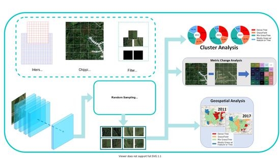
1. Introduction
The remote sensing field has seen rapid development in recent years, which has resulted in a deluge of overhead high-resolution imagery from airborne and spaceborne remote sensing platforms. Although this huge data provides plentiful new sources, it far exceeds the capacity of humans to visually analyze and thus demands highly automatic methods. This data volume has also seen continual enhancements in temporal and spatial resolution of remote sensing information [1,2,3,4,5,6]. These circumstances necessitate the development of new human–machine teaming approaches for visual imagery analysis workflows, specifically techniques that leverage state-of-the-art computer vision and machine learning. This increasing amount of geospatial big data are utilized in a key task in the earth observation, change detection (CD), which is one of the most active topics in the remote sensing area due to the persistent occurrence of catastrophes such as hurricanes, earthquakes and floods [6,7,8,9], in addition to the interactivity of human with natural phenomena [10]. The objective of CD is finding the change in the land cover utilizing co-located multitemporal remote sensed images [11]. It is a key technology that has been investigated in many fields such as disaster management, deforestation, and urbanization [7,12].
More abundant details of geographical information can be acquired from the high spatial resolution (HSR) images that can be obtained from various sources for example IKONOS, QuickBird, and WorldView [13]. Thus, high resolution images are in demand or imperative for various remote sensing fields [14]. However, the improvements of spatial resolution conveys challenges to automated change detection processes [15]. Generally, change detection methods fall under three categories, traditional pixel-based change detection (PBCD), object-based change detection (OBCD), and hybrid change detection (HCD) [15].
Pixel based methods [16,17,18] compare the multitemporal images pixel-by-pixel. There are many traditional pixel-based algorithms, such as image differencing, image rationing, principal component analysis (PCA), and change vector analysis (CVA). Using isolated pixels as the basic units in the pixel-based methods results in a over-sensitive change detection [13]. Additionally, they can be affected by noise, in particular, when handling the rich information content of high resolution data [19]. For the object-based methods [20,21,22,23,24], first a segmentation procedure is applied to extract the features of ground objects. Next, using an object-based comparison process the change map is obtained. The final result of OBCD is usually sensitive to the segmentation process [13]. Existing HCD techniques have proven suboptimal as well [25,26], in so much as the classical HCD methods belong to intuitive decision-level fusion schemes of PBCD and OBCD [13].
In addition to the above three categories the change detection can be gathered into two categories from the view of the ultimate aim, binary CD methods and multitype CD methods. While binary CD emphases highlighting the change, multitype CD objectives is to differentiates various types of changes [27]. In this paper, we propose a new approach for change detection, which is a chip-based approach facilitating multitype CD. This chip-based approach enables analysis at a variety of geospatail levels-of-detail; from chip-level change analysis up through larger spatial region analysis.
Feature learning is an efficient approach to represent imagery data [28]. The literature shows that the deep learning based feature extraction demonstrates superior generalization properties that allow us to take advantage of the abilities of the transfer learning. In this scenario, the knowledge that is gained from a deep network that is pretrained on one domain can be transferred to other domains. Those features that are extracted from the deep networks, a.k.a. deep visual features, are proven to have more robust domain invariance ability in the remote sensing field than the features extracted from shallow networks [29,30,31,32,33]. Additionally, deep features have the advantage of capturing the spatial context information efficiently [29,30,31,32,33].
In the architecture of CNNs, convolutional layers and pooling layers are stacked interchangeably for feature extraction. The CNN-based deep model structure makes it significantly appropriate for feature learning of images, which is capable of overcoming the deformation of spatial features caused by rotation and translation [34]. Several researchers have utilized convolutional neural networks (CNN) to extract features from satellite data for a variety of use cases. Li et al. [35] proposed a deep CNN-based method for enhancing 30-m resolution land cover mapping utilizing multi-source remote sensing image. The CNN-based classifier is employed to extract high resolution features from Google Earth imagery. Zhong et al. [36] built deep neural networks with numerous architectures to classify summer crops utilizing EVI time series.
Zhang et al. [37] combined the local information extracted by histogram of oriented gradients (HOG) along with the CNN features representing contextual information. They utilized a CNN model trained on ImageNet (ILSVRC2012) as the contextual feature extractor. In [38], the authors trained a CNN to label topographic features, such as roads, buildings, etc. In [39], features and feature combinations extracted from many deep convolutional neural network (DCNN) architectures were evaluated in an unsupervised maner, then leveraged for classification of the UC Merced benchmark dataset. The authors found that both ResNet and VGG have design parameters that work well with spatial data.
In real-world application, data usually contain complex many-to-many relationships [40]. To detect the multi-type change, the data should be clustered first. Various image clustering algorithms have been utilized as an unsupervised pattern recognition technique for different tasks involving HR-RSI. Fuzzy c-means (FCM) is one of the soft computing techniques in which each data point has a degree of membership in each cluster [41]. That makes it a well suited approach for HR-RSI because image chips may have complex composition, such as trees, grass, roadways, buildings, water bodies, and more.
In the age of Big Data, it is no longer necessary to constrain broad area analysis to coarse and low-resolution geospatial data. One of our key contributions is to highlight how the details and features in the visual present within high-resolution imagery can be utilized to tease out the differences between various clusters. In lower resolution imagery, small individualized details are barely discernible as visual features. Importantly, automated methods that can detect these subtle changes can capture importing aspects related to change, such as subtle tree removal operations that are not clear-cut lumber harvests.
The main contributions of this paper can be summarized as the following:
- A chip-based approach has been proposed for multi-temporal change detection. The beauty of the proposed approach is that, unlike state of the art methods, it supports detecting the change in a large scale area with massive amount of HR remote sensed imagery data, while also facilitating higher resolution level-of-detail analysis. In other words, our proposed method gives an insight into the distribution of each cluster within the study area as a single unit, as sub-areas represented by the census blocks, and at the local chip level. Additionally, it overcomes the challenges of unaligned and multi-resolution corresponding imagery.
- Generation of orthogonal deep visual features utilizing a DCNN along with the transfer learning techniques to extract the deep features for change detection analysis, considering the deep features represent the remote sensing data better than the traditional features extraction methods. Additionally, we project the DCNN extracted features into an orthogonal space preserving most of the information for enhanced unsupervised machine learning utilization. This solves a key challenge in the real world applications, as sufficient training data is not always available.
- Soft clustering based on fuzzy c-means algorithm has been utilized to aggregate small image patches of similar visual composition. This is because the surface of the Earth is not composed of crisp distinctions of land cover in the high-resolution domain. Instead, any local image patch could be a mixture of various land cover types. Fuzzy c-means can capture this characteristic efficiently by the means of the soft partition.
- Three analysis methodologies are introduced: cluster analysis, geospatial analysis, and metric change analysis. To successfully analyze the varied resolution images, that may be misaligned, change in the sub datasets is computed at the chip level using a neighborhood approach.
The remainder of this paper is organized as follows. Section 2 describes the datasets and the preprocessing stages. Section 3 presents our approach for extracting visual features from deep neural models that feed into a dimensionality reduction and soft partitioning. Section 4 details our analysis methodologies of the proposed approach. Section 5 outlines the experimental setup and presents the results. Section 6 interprets and describes our findings. Finally, Section 7 concludes the research and highlights future directions.
2. Datasets and Preprocessing
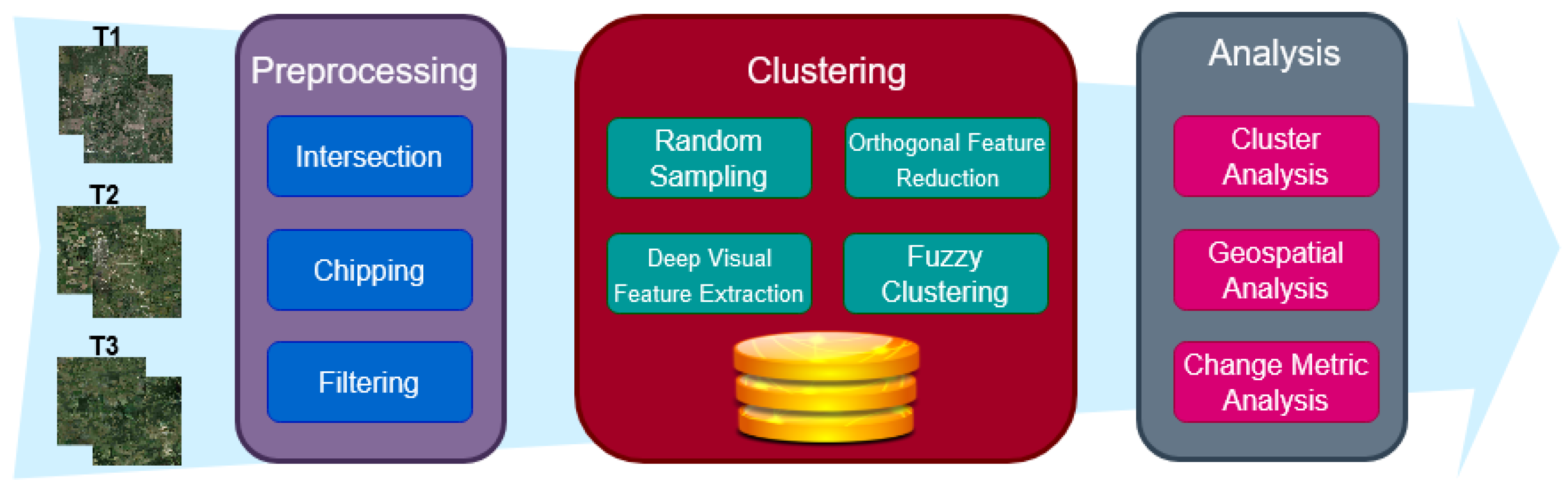
In this section, we describe two datasets and our preprocessing steps. The general workflow of this research is shown in Figure 1, and Table 1 lists the symbols used in this research.
2.1. Datasets Description
In this research, two main datasets were utilized. First, a publicly available benchmark dataset is used to train the deep neural feature extractor. The second dataset is our study area encompassing Columbia, MI, USA and the surrounding areas, including three different years.
2.1.1. RSI-CB256 Benchmark Dataset
The Large Scale Remote Sensing Image Classification Benchmark via Crowdsource Data (RSI-CB) [42] is used in this research to train the deep neural feature extractor. Specifically, the pixel sub dataset (RSI-CB256). According to the authors, it is 0.22–3 m GSD, which makes it higher spatial resolution than many other existing datasets. Higher spatial resolution means higher information details.
The authors collected points of interest (POI) from Open Street Map (OSM), which directed the imagery scraping from Google Earth and Bing Maps. In total, there are 24,000 images across 6 categories with 35 subclasses including town, stream, storage_room, sparse_forest, snow_mountain, shrubwood, sea, sapling, sandbeach, river_protection_forest, river, residents, pipeline, parkinglot, mountain, marina, mangrove, lakeshore, hirst, highway, green_farmland, forest, dry_farm, desert, dam, crossroadsbridge, container, coastline, city_building, bridge, bare_land, city_avenue, artificial_grassland, airport_runway, airplane. The major countries where the POI were chosen from include USA, China, and UK [42]. The RSI-CB dataset is an imbalanced dataset; some classes consists of more than 1300 image while other less than 200 images. Thus, data augmentation was a vital for our research to get a better performance.
2.1.2. CoMo Dataset
The second dataset consists of three subsets of raster data. Each subset corresponding to a different year. Table 2 summarizes the properties of this dataset. The datasets have been collected over the following dates 5 April 2011, 10 October 2015, and 4 May 2017.
Of note, the tiles at the edges of the scanned area have different spatial extents than the rest of the tiles. This is true for the three sub-datasets. Additionally, the 2011 dataset is neither aligned nor has the same resolution as the other two datasets.
For the sake of this research, each tile is divided into 256 × 256 pixel chips to be consistent with the images of RSI-CB256 dataset. Each regular tile yields 4096 chips, which is a significant amount of data; more than 108 billion pixels in 2011 dataset and more than 24 billion pixels in each of 2015 and 2017 datasets. Handling such data at pixel-level is extremely computationally expensive, without a commensurate value in the resulting pixel-wise output. In this way, the chip-level approach, in the combination with DCNN features extraction, represents a suitably efficient data analysis technique that balances resolution of analysis (level-of-detail) with computational costs.
2.2. Region Imagery Preprocessing
To detect the change in the area of the interest, the three temporal subsets of the CoMo data should cover the same area. However, as can be perceived from the range of the geographic coordinates, the year 2011 covers different area than 2015 and 2017. This is a common problem with large-scale remote sensing datasets. Specifically, datasets that are collected over various years. The change analysis is limited to only the overlapping sub-area among the analyzed datasets. Using the accompanying geospatial polygons from the data provider, we are able to intersect the overlapping area and trim each year of the CoMo dataset to an appropriate set of scene tiles. This intersected geometry represents the final study area.
For the purpose of this research, each tile is partitioned into several chips of equal size, chosen to be 256 × 256 pixels for consistency with the RSI-CB256. Thus, each regular tile yields about 4096 chips. It is worth noting that the tiles at the edge of the scanned area are not always the same size of the regular tiles based on the source imagery capture; and therefore may yield a lower number of chips.
In this research we are interested in the center location of each chip. Thus, we defined Equation (1a,b) to obtain the center of each chip from its upper left corner. This equation assumes the scene, tiles, and chips are north-up.
As mentioned, the size of the tiles at the edges are not the same size of the regular tiles, therefore, some chips at the very edges have partial information. These chips are not useful and could negatively affect the subsequent processing and are therefore filtered out.
Algorithm 1 shows the pseudo code that checks if the chip is NoData chip or not. If it is NoData chip we will exclude it from further processing. First, the size of the chip is compared against a predefined threshold. If it is less than the threshold, it could be a useless chip that needs to be excluded. To make sure this chip does not contain useful information, it is compared at the pixel level to check whether most of the pixels in the chips are NoData or not. Comparing the size of the file first helps with expediting the process as comparing all the chips in such big data is computationally expensive.
Table 3 lists the details of the intersected area after the preprocessing. The 2011 datasets is slightly different than the other two datasets even after the processing because we are targeting the chip level and these data are not aligned with other two datasets. However, this difference is a result of spatial intersection of the sub-scene tiles with respect to the geospatial extent of the study area, where the tiles of the 2011 scene extend from the polygon different from the 2015 and 2017 scenes. In the case of all three subsets of the CoMo data, the chips are further refined to both remove chips out of the extent as well as remove chips with significant NoData values. Furthermore, notice that the number of the chips in the intersected 2011 dataset is higher than the other two datasets due to the higher pixel resolution of this dataset. These characteristics highlight two particular challenges of the CoMo datasets—and many other large-scale multi-temporal datasets—that our methods detailed in Section 4 sufficiently handle. First, the data is of varied resolution and it is not necessary to resample the data to uniform spatial pixel resolution. Secondly, our methods will accommodate data that is not perfectly aligned, which is often a necessary condition of PBCD and even many OBCD.
| Algorithm 1: Filtering out the NoData Chips |
 |
3. Deep Visual Feature Extraction and Clustering
This section describes the deep feature extraction, transformation to orthogonal visual features for reduced dimension, and clustering. Algorithm 2 details the process, along with the subsequent Section 3.2 and Section 3.3.
3.1. Deep Neural Feature Extraction Training
As mentioned previously, deep learning has proven its superiority in extracting the features over hand-crafted methods. In this research, the ResNet50 [43] DCNN model is trained with the RSI-CB256 dataset after transfer learning from the ImageNet dataset [44]. The most remarkable characteristic of ResNet is depth [45].
The RSI-CB256 dataset is an imbalanced dataset; some classes consist of more than 1300 images while others less than 200 images. The data are divided into three subsets: training, validation, and testing leads to low performance. For this reason, preprocessing is a mandatory requirement. First, the data have been shuffled to avert any bias. Next, to avoid overfitting, the oversampling has been done after dividing the data into training, validation, and testing. This will guarantee there is no duplication in the data across the three subsets. The image rotation is used in oversampling the data. The images have been rotated in various angles including the following ranges [0–7, 83–97, 173–187, 263–277]. These ranges have been chosen to avoid losing the information from the image in case it rotated with large angles. In each subset, the classes have been oversampled to be equal to the largest class in the subset. Furthermore, the training dataset has been horizontally flipped, zoomed, cropped to avoid overfitting.
During training with RSI-CB256, the last convolutional layer is fine-tuned along with the training of the new classification phase to ensure the resulting features are adapted from the ground photo to the overhead imagery domain. The resulting DCNN generates 2048 deep visual features that are then assembled into 800 higher-level features (i.e., hidden layer) within the multilayer perceptron (MLP) classification phase before the final softmax node classifier output (see [46] for further details).
To ensure the proper training of the DCNN, the RSI-CB256 was organized into a 60/20/20 percent training, validation, and blind testing split. After training, the validation and blind test sets had classification performance of 98.72% and 99.31%, respectively. Figure 2 shows the validation and testing Confusion matrices for the RSI-CB dataset. As the figure reveals, all the matrices contain the data around the diagonal line, which confirms the classification performance result. The activations of the 800 node hidden layer are the extracted deep visual features in this research (Algorithm 2, line 3 and 14).
3.2. Deep Orthogonal Visual Features
With 800 deep visual features, there is the potential for much redundant information, and therefore we utilize PCA to reduce the feature space (and the associated memory and computation requirements). We leverage PCA to minimize information loss during feature reduction (Algorithm 2, lines 6–7 and 24–25). PCA reduces numerical redundancy by projecting the original feature vector to a lower subspace, minimizing information loss [47]. Additionally, in the context of clustering driven by high dimensional dissimilarity metrics, reducing the effects related to the curse of dimensionality can improve the derived clusters. In this research, we reduce the deep visual features to 108, 110, and 102 dimensions for years 2011, 2015, and 2017, respectively; in each case preserving 99% of the data variances. These deep orthogonal visual features are then suitable for cluster analysis and other unsupervised machine learning methods that leverage metric spaces. We randomly sample the study area (30%) to derive the principle components and the reprojection eigenvectors, which is then applied to the entire study area.
| Algorithm 2: Feature Extraction and Clustering |
 |
3.3. Fuzzy Land Cover Clustering
As with any large swath of remote sensing imagery, our study area is inherently non-discrete. This is especially true of high-resolution imagery, where small objects (visual features) are discernible and the composition of a collection of visual features within a local spatial extent drive the assessment of that localized area. These visual features may include trees, areas of grass, buildings (or other impervious surfaces), water, and more. In this research, the computational locality is at the chip-level, as defined in Section 2.2. To facilitate large-scale analysis when the potential variability of the chip content is so diverse, we leverage soft-computing techniques. Specifically, we employ the fuzzy c-means (FCM) method, Ref. [48], to generate a soft partition of data into groups of similar visual content.
Within the FCM model, each data point (chip) is measured for similarity to cluster centroids to generate a cluster membership in [49,50]. Each chip’s deep orthogonal visual features are measured against the center of each cluster using Euclidean distance to form a partition matrix, u. The FCM algorithm oscillates between computing weighted mean positions (center of mass) for each cluster and updating cluster memberships (the fuzzy partition matrix). Similar to the development of the deep orthogonal visual features, we leverage a 30% sample to learn the cluster centers in the deep orthogonal visual feature space. The final cluster centers are then used to compute a final u. The FCM algorithm is Algorithm 2, line 8 that trains the FuzzModel. Algorithm 2 line 26 uses this model to label all chips into the learned clusters.
The fuzzy partition matrix is utilized to create soft labels of the study area chips. Specifically, each chip’s strongest cluster membership is extracted as both a label and a membership degree; thereby making the information better aligned for geospatial visualization and human interpretation.
The fuzzy partition matrix u is reduced to firm labels with membership via Equation (2).
where is the individual membership of chip j in cluster i, is the number of clusters, and N is the number of data points. The resulting tuple vector encodes the cluster assignment for each chip while preserving its membership information.
The unsupervised machine learning methods, such as fuzzy clustering, are usually very data dependent. Due to variability encountered in seasons, atmosphere, and sun/sensor geometry, we cannot expect unsupervised methods to generate data labels (i.e., cluster labels) that are coherent across scenes. For this reason, we aggregate the clusters into key semantic classes that dominate our study area: dense tree, grass field, mixed grass and tree, and mostly grass with tree or feature. This semantic grouping allows the mapping of any scene into numerically comparable chips. The grouping can be determined from any clustering with greater than the number of semantic categories. After mapping each group of clusters to its target semantic category, the partition probabilities of each group members have been added together to produce the final partition probability of the target semantic category.
4. Analysis Methodologies
In this section, we present our methodology for cluster, geospatial, and change metric analysis.
4.1. Cluster Analysis
To explore the study area and detect the changes over the time period from one year to another, the clustering results are analyzed in this section. The percentage of each cluster in the study area has been calculated using Equation (3).
while the percentage of the change per cluster in CoMo and the surrounding areas has been calculated according to the Equation (4)
Since the study area covers a broad region, we can examine it at a compositional level-of-detail, such as census blocks. Thus, the cluster of the whole study area is a union of all the clusters of type i in each block, which can be defined as follows:
In essence, we can agglomerate any arbitrary sub-region at a broad range of spatial extents (number of chips) to facilitate analysis at numerous levels-of-detail. In some situations, it is desirable to investigate a small, localized area such as a census block for monitoring scenarios. Therefore, each block can be analyzed individually to understand the change per block, potentially combining this with any number of other geospatial layers that are often aggregated to the same level-of-detail. The following formula (Equation (6)) is used to calculate the percentage of each cluster per block.
The percentage of the change in each cluster per block in a specified period of time has been calculated utilizing Equation (7). The output of this equation could be positive or negative. The positive output indicates that the cluster has been increased within that block while the negative output indicates that the cluster has been decreased within that block.
4.2. Geospatial Analysis
In addition to the cluster analysis, the geospatial analysis is yet another vital analysis, especially for Geographic information system (GIS) applications. It is very important to present the clusters on the geographic map, which helps to explore the change by linking the clusters and the census blocks on the maps of various years.
Each census block is compromised of numerous chips, where each chip could belong to a different cluster. As the aim is to represent each block in the geographic map using one color that represents a dominant cluster, we must compute the dominant cluster within the block. For this purpose, we have developed a method based on the fuzzy partition partition (Equation (2)). Generally, by representing the block using one cluster there will be some loss in the information.
However, the purpose here of the geographic maps is to provide an abstract view of the clusters and link them to their geospatial extents on the surface of the Earth. In fact, representing a summary of clusters facilitates capturing the nature of the Earth since we are dealing with large-scale data and hundred of thousands of datapoints (localized chip spatial extents). In contrast, is it very difficult for humans to consume the information or recognize the clusters and the nature of the area of interest when all the datapoints are rendered on the map without summarization.
The proposed method, Equation (8), utilizes the membership degree of the fuzzy clustering (Equation (2)). For each cluster within a block, the average of the membership degree for all chips is calculated, then the cluster with the maximum average of membership degrees will be chosen to represent that block.
4.3. Change Metric Analysis
Another important analysis is measuring the magnitude of the change in a time period based on the membership degree of a chip. For this purpose, we have utilized two methods. The first method uses norm2 and the second uses Jensen–Shannon divergence (JSD).
The data of 2011 is not aligned geospatially with the data of 2015 and 2017. Therefore, measuring the change between the data of the years 2011 and 2015–2017 is not a straightforward process. Algorithm 3 provides an efficient geospatial neighborhood search technique, such that analysis can be performed using very small, localized sets of chips. The neighborhood algorithm is utilized to find the neighbors of each chip in the year we want to compare with. First, the radius is determined, which is the spatial aperture of analysis, such that it determines the area to search for the neighbors of each chip. Second, the approximate nearest neighbors are found from the spatially indexed chips. Third, the Harversine formula (see Equation (9a,b)) is used to find the final neighbors within the specified radius on a sphere (surface of Earth) for each chip based on geospatial coordinates for a given maximum distance. Algorithm 3 shows the pseudocode for the neighborhood method utilized in this research.
| Algorithm 3: Geospatial Neighborhood Search |
 |
The Haversine formula (Equations (9a,b)) is a simplified version of the arcsine form of the cosine law for a sphere utilized in the calculation of great circle distance. Great circle distance is used to measure the shortest distance between two points on the surface of the Earth. Though, as a result of the arcosine form of the cosine law on the sphere, the great circle distance calculation formula has a large error at a small distance. The substituted form is Haversine formulas, which produces a more accurate solution on the calculation of the smaller distances [51].
After finding the neighbors of each chip, norm2 () is calculated to define the amount of the change during a specified period of time at the chip-level (Equation (10)). The average of the neighbors’ membership have been calculated first. Then, norm2 of the difference between the two vectors of the average fuzzy partition have been measured according to the Equation (10).
Another method that has been used to calculate the change metric is Jensen–Shannon divergence (JSD). The JSD (a.k.a. information radius (IRad) or total divergence to the average) is a well-known method for calculating the dissimilarity between two probability distributions. Note, that by definition of the FCM algorithm, the cluster memberships for a chip will sum to 1.0; and can be treated analogous to a probability. JSD can be considered as a symmetric and bounded version of Kullback–Leibler divergence [52,53]. Equation (11a–c) shows the formula to calculate JSD.
subject to
where
stands for the Kullback–Leibler divergence and can be calculated utilizing Equation (12).
5. Experimental Results
In this section, the analysis results that are obtained based on the methodologies described in Section 4 are presented.
5.1. Clusters Analysis Results
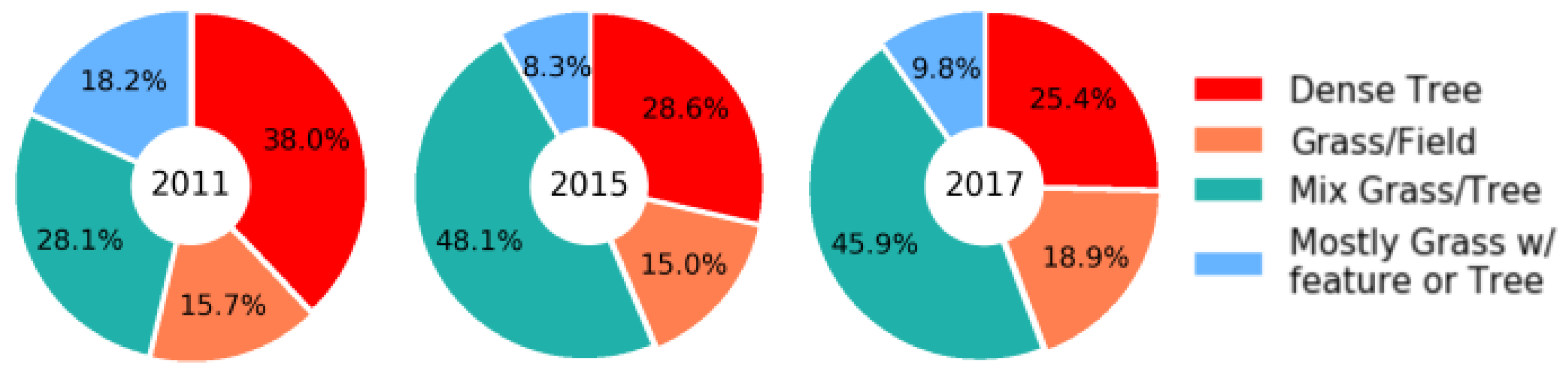
The cluster analysis provides an insight into the distribution of each cluster within the study area either as a single unit or as sub-areas represented by the census blocks. The cluster analysis could serve as the exploratory step to the change detection process since it is important to know the division of the study area based on the type of the cluster to be able to compare and conclude the multi-type change. Figure 3 shows the percentage of each cluster for the study area.
As mentioned previously, since this research targets a large scale area, it could be vital in some circumstance to investigate subareas. Therefore, the region has been explored based on the census blocks level as well. Each block is compromised of more than one cluster with the exception of some blocks that consist of only one cluster. This due to the fact that most of the blocks cover significant geographic areas.
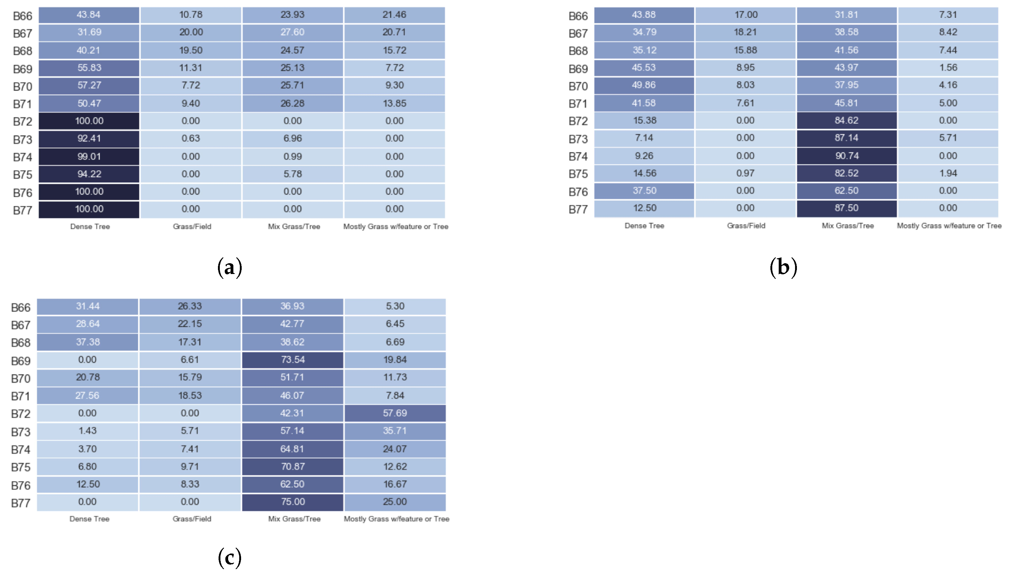
Figure 4 shows a sample of the percentage of each cluster per block in the three years 2011, 2015, and 2017. In Figure 4a, the top six blocks represent a diverse cluster with a strong Dense Tree and then transitional areas of grass and trees; and the lower six blocks are a cluster that is dominated by Dense Tree. In Figure 4b, the top six blocks represent a diverse cluster with mostly Dense Tree and Mix Tree/Grass; and the lower six blocks are a cluster that visually exhibits mostly areas of Mix Grass/Tree and little to no open grass fields. In Figure 4c, the top six blocks represent a diverse cluster with mostly Mix Tree/Grass and little of Dense Tree and Grass/Field; and the lower six blocks are a cluster that visually exhibits mostly areas of Mix Grass/Tree and little of Mostly Grass w/feature or Tree.
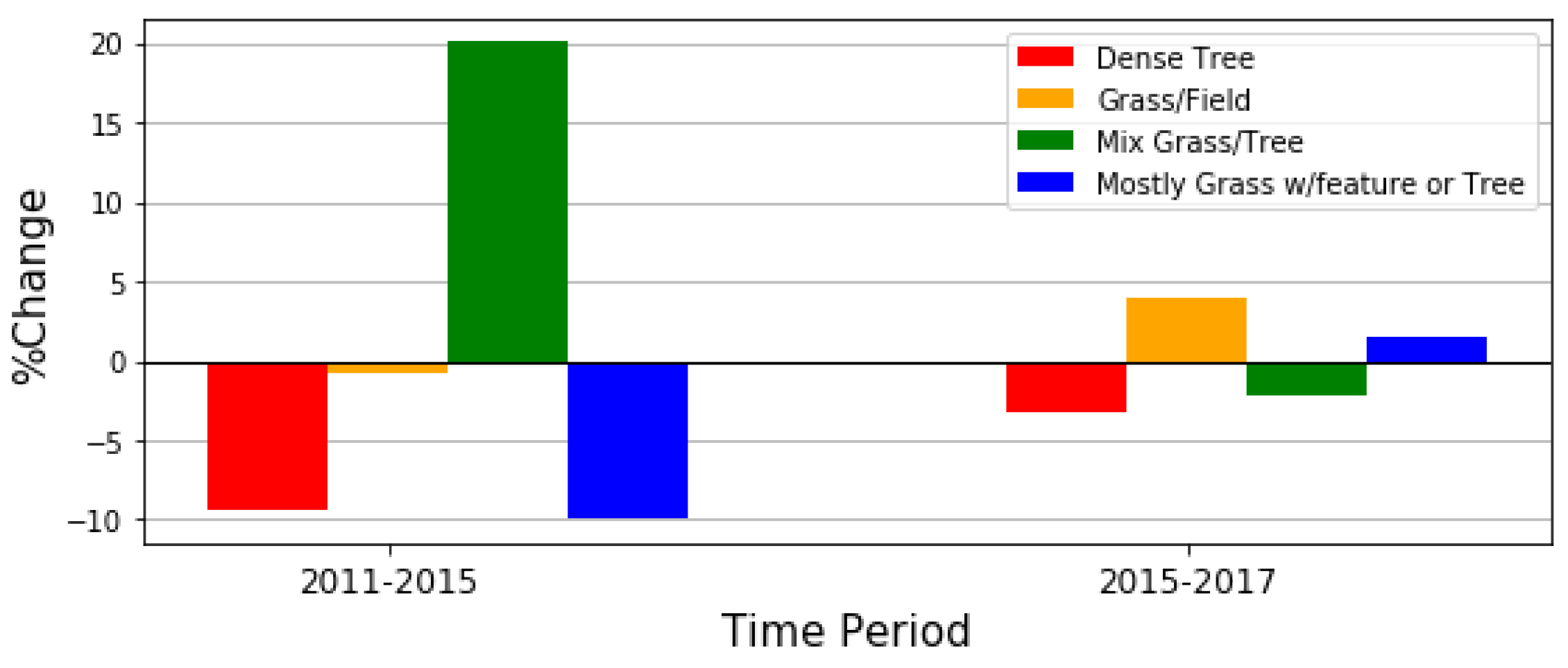
The percentages of the temporal change per cluster in the whole study area for the two time periods, 2011–2015 and 2015–2017, are shown in Figure 5. Some clusters increased while some other decreased. For instance, during the period 2011–2015, three clusters, dense tree, grass/field, and mostly grass w/features decreased by about 9.34%, 0.71%, and 9.95%, respectively; while mix grass/tree increased with the percentage of 20%. Additionally, it can be seen there is a small change during the time period 2015–2017 compared to the other period since it is a smaller temporal window. The figure clearly shows that the dense tree cluster, unlike the other clusters, constantly decreases in both periods; which can be expected in a study area such as this with expanding suburban characteristics encroaching on undeveloped rural areas.
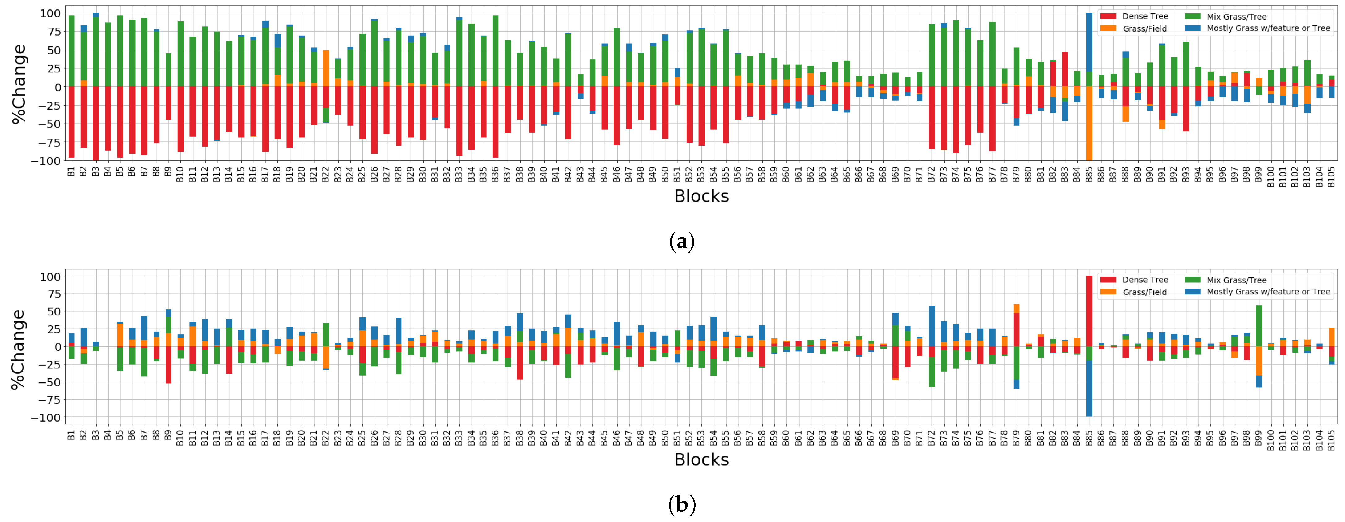
The stacked change of each cluster in each block is illustrated in Figure 6. In general, the trend in the change per block agrees with the change in the CoMo data as a whole (Figure 5). However, the block level provides more details about the change. For example, in the period 2011–2015, the grass field increases especially in the blocks B17–B62 while it decreases in most of the blocks on the right side of the figure. Additionally, it can be noticed that some blocks did not change at all, such as B4 in Figure 6b.
5.2. Geospatial Analysis Results
Visualizing the clustered data on the geographic map is yet another method for exploring the change, using the geographic location and a predesignated subdivision such as census blocks. In fact, rendering clusters on the map facilitates understanding the actual spatial extent of the change on the surface of the Earth. The proposed method introduced in Section 4.2 is utilized to visualize the clustering results on a map. Recall the purpose of these maps is to provide a summarized view of the change, thus each census block is represented by the predominant cluster only, although the majority of the blocks consist of more than one cluster. This process sacrifices some of the detailed information, unlike the other detailed analyses performed in this research. Indeed, our aim in rendering the clusters on the geographic map is to summarize the information for a clearer synoptic view.
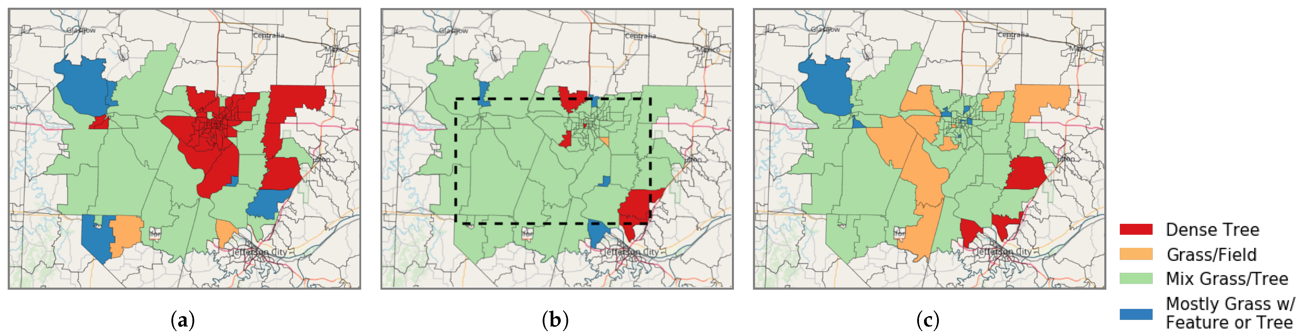
Figure 7 shows the geographic map of the three studied years. In these maps, where the map is based on the block level, the whole block is labeled based on the predominant cluster even if just partial data of the block is available. The actual study area is surrounded with black dashed rectangle in Figure 7b and this is the same study area for the years 2011 and 2017. The blocks that are partially inside the study area are based on the partial information; while the blocks that fall completely inside the study area have complete information for said blocks.
5.3. Change Metric Analysis Results
This subsection details how to measure the magnitude of the change based at the chip-level utilizing the methods demonstrated in Section 4.3. As the volume of data data increases, we need an intelligent metrics to measure the change efficiently. A promising solution is to measuring the divergence between two distributions. Researches [54,55,56] have used many metrics to measure the similarity such as the Kullback–Leibler (KL). However, to measure the change we need symmetric metrics. Thus, to measure the magnitude of the change, we have utilized the symmetric metric Jensen–Shannon divergence (JSD) in addition to norm2 (L2). For both metrics we utilized a neighborhood method to get the corresponding area in the referenced year. Two approaches for the neighborhood method implementation have been investigated:
- 1–N: compares the chip in a base year to the corresponding neighbors (average) in a later year.
- M–N: compares the corresponding neighbors (average) of a chip in a base year to corresponding neighbors (average) in a later year.
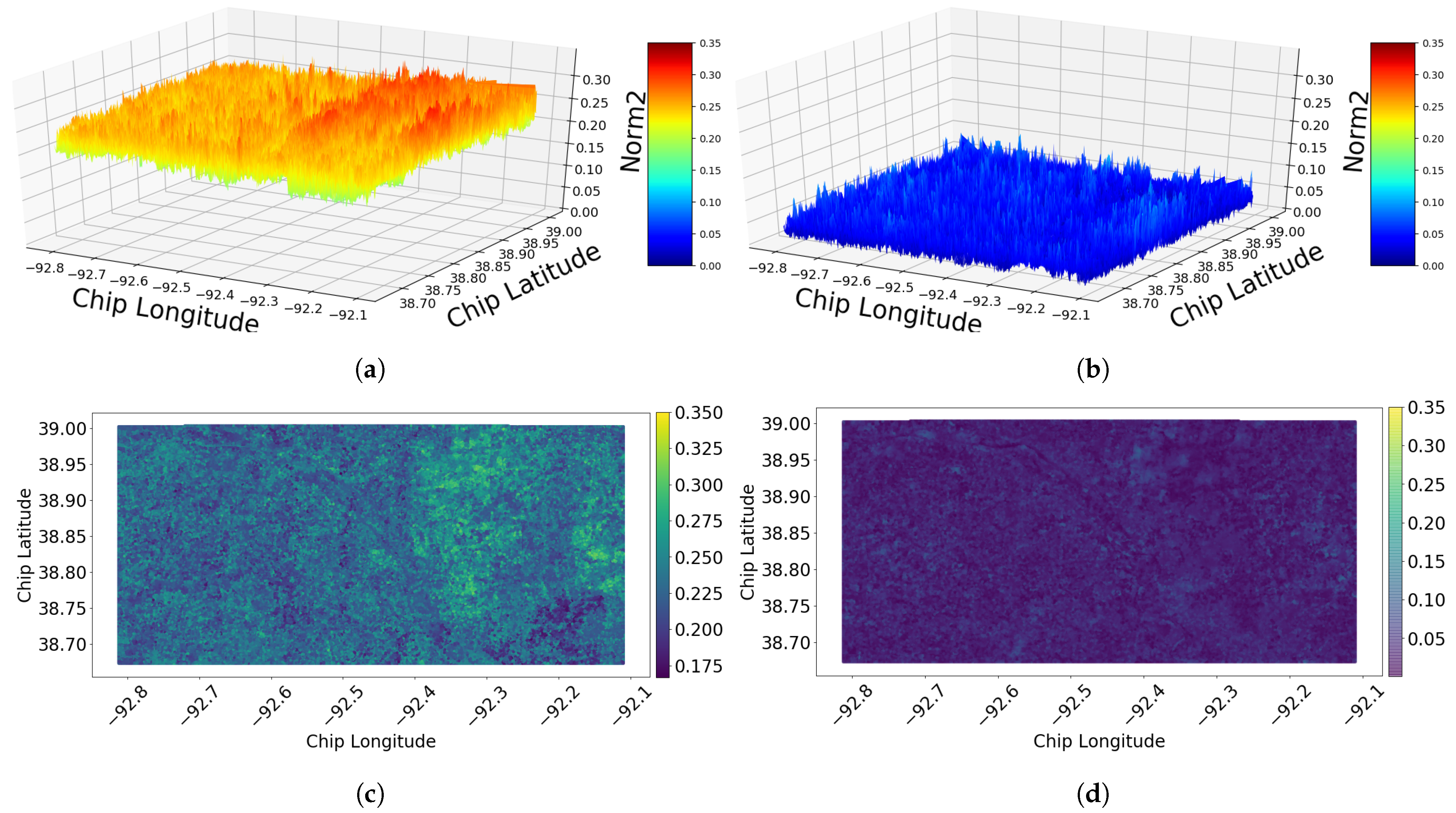
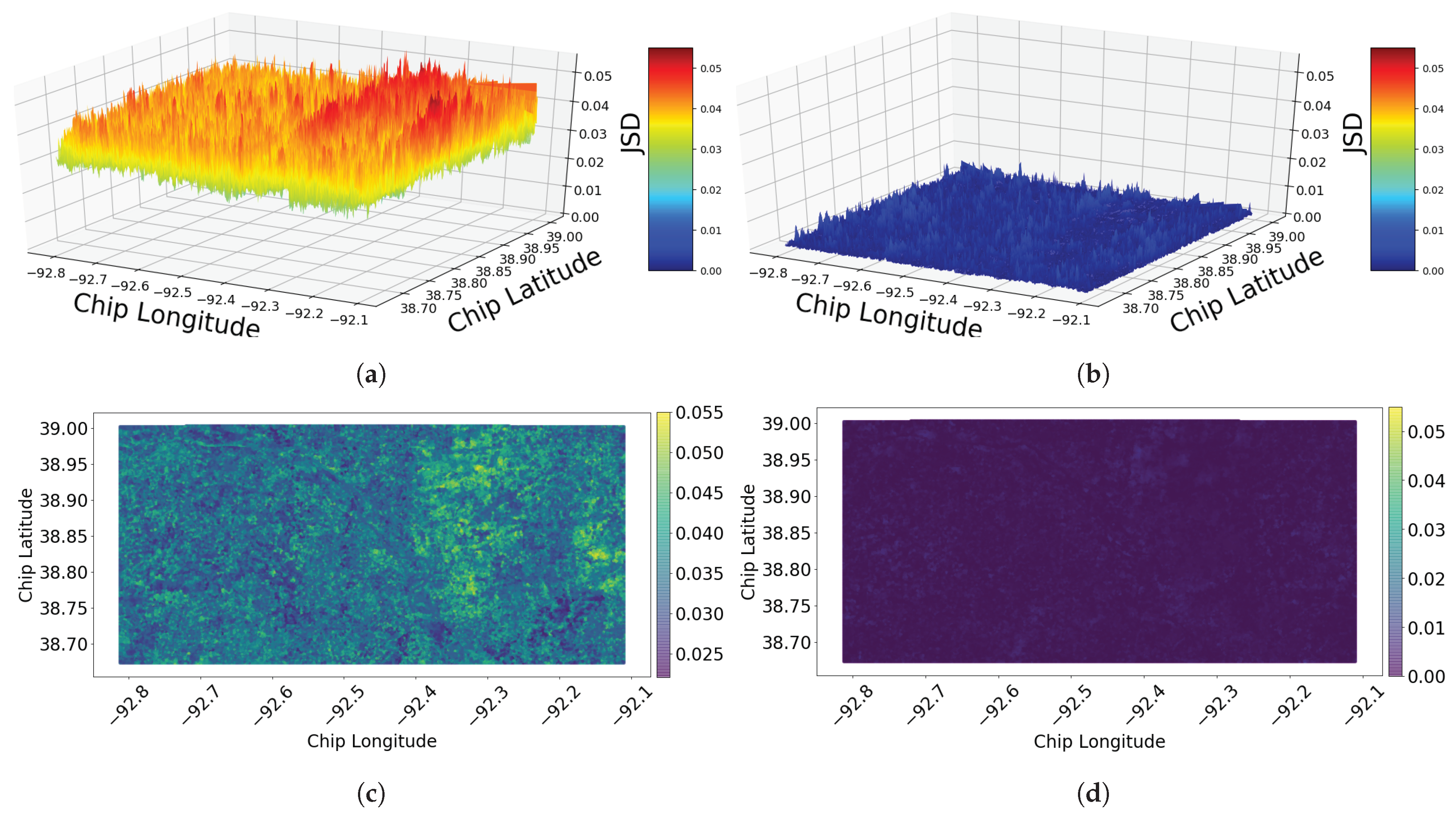
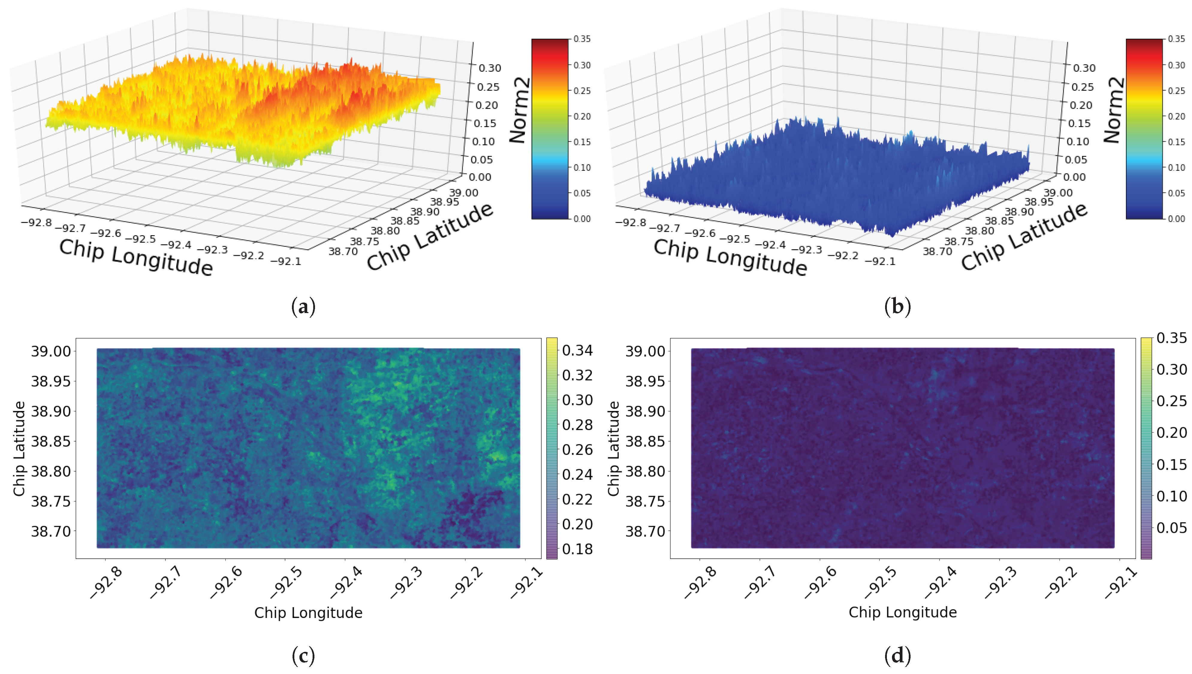
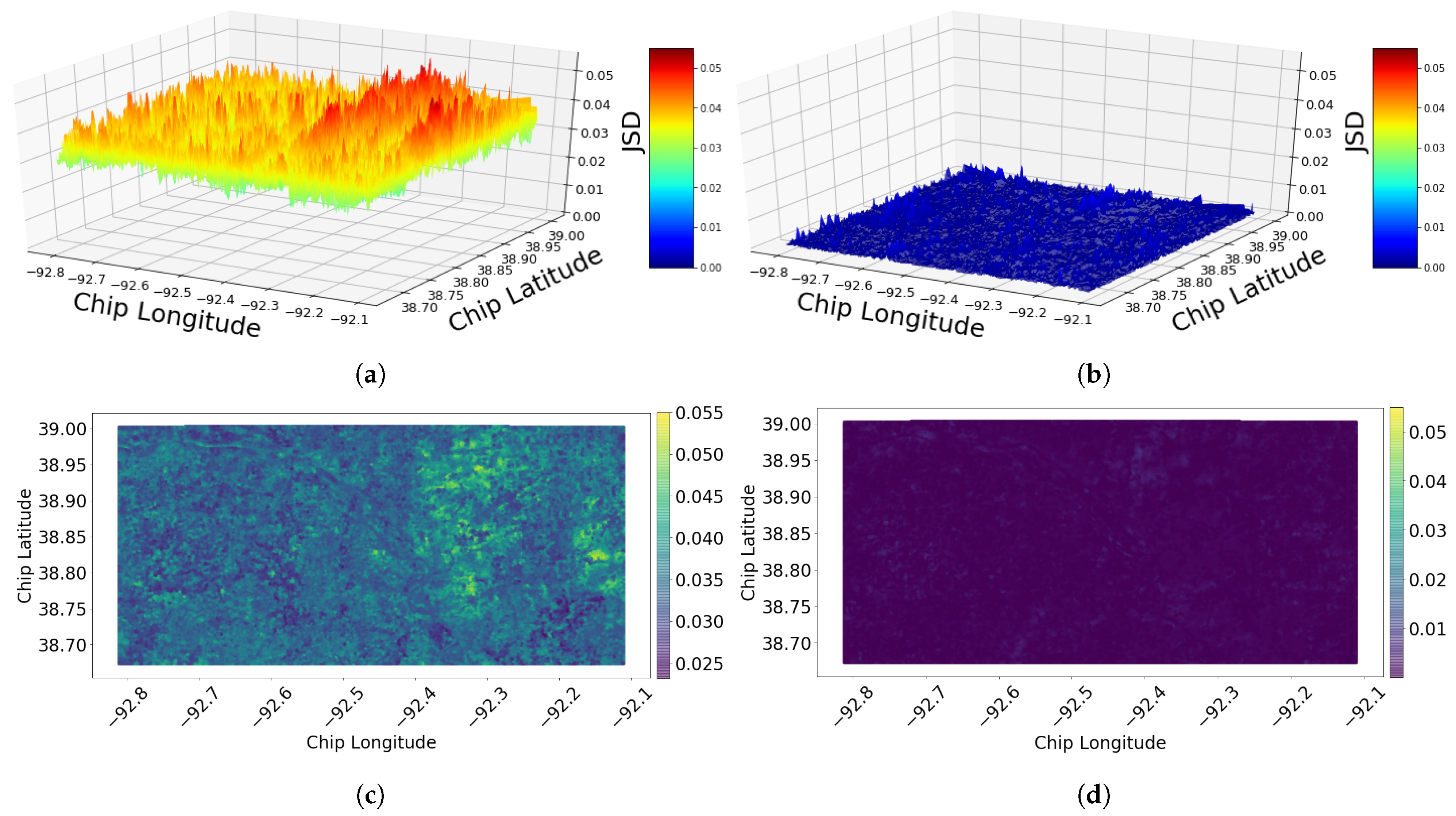
For the first approach, 1-N, Figure 8 shows norm2 of two time periods 2011–2015 and 2015–2017. It is clear from the figure that the amount of the change of the first period (2011–2015) is more than the amount of the change of the second period (2015–2017). This supports the results in Section 5.1, which details the percentage of the change. The second change metric utilized in this analysis is JSD. The similarity of the results obtained from JSD (see Figure 9) and the ones obtained from norm2 is as expected.
For the second approach, M-N, the results of norm2 and JSD are shown in Figure 10 and Figure 11, respectively. It is worth mentioning here the distance value has been chosen to include the neighbors that are defined based on the Moore neighborhood (potential chip plus its direct vertical, horizontal, and diagonal neighbors).
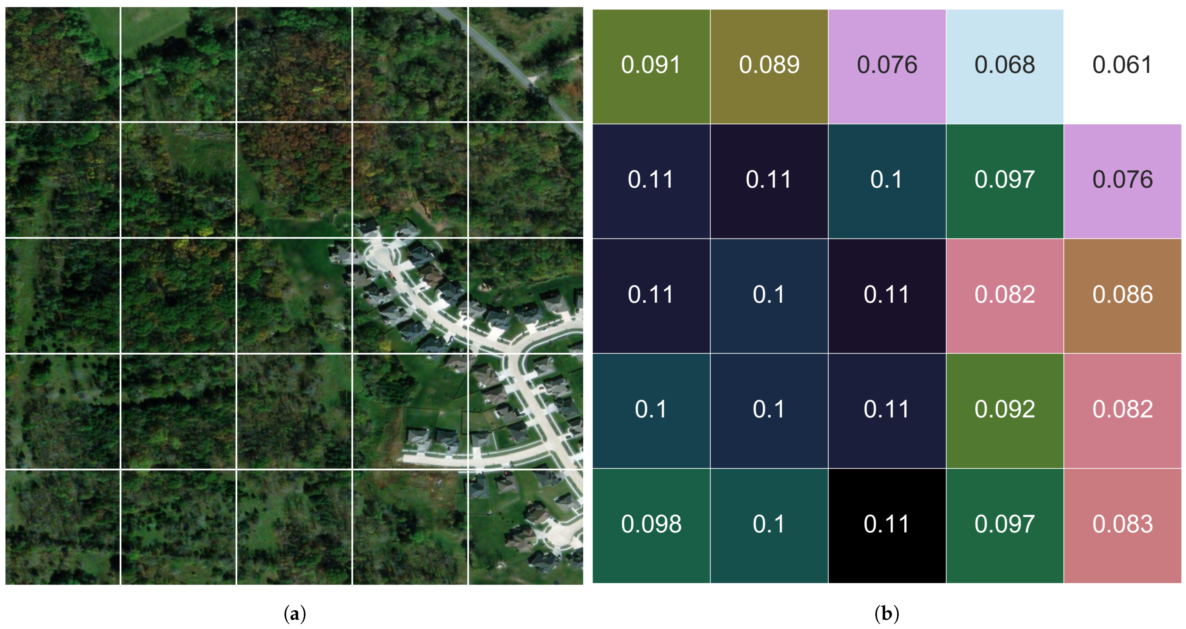
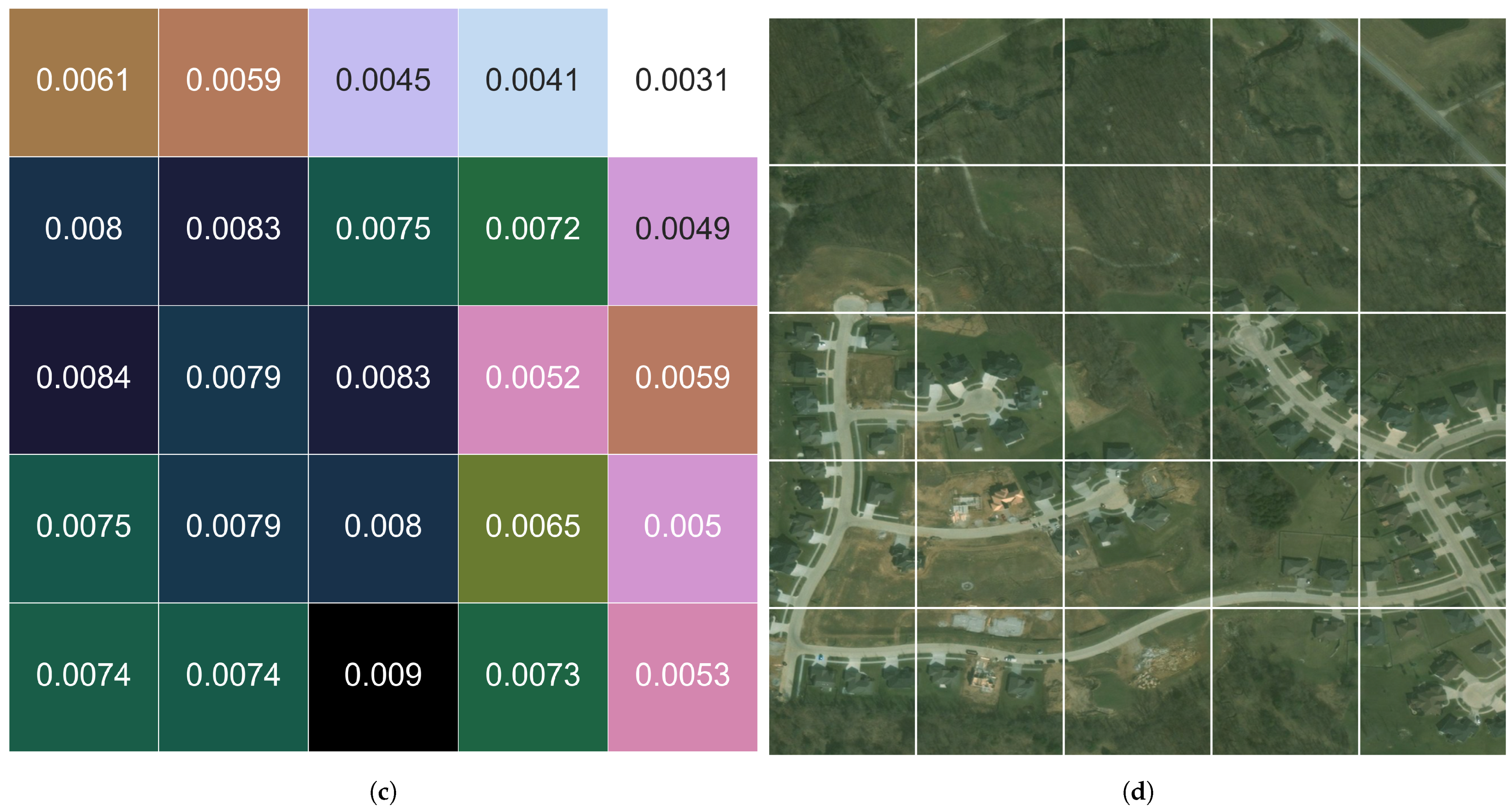
Figure 12 illustrates the change detection in a sampled set of chips for the time window 2015–2017 utilizing the 1–N neighborhood method. The new construction (removal of trees along with the addition of road and houses) represents ground-truth visual change that measures higher than the surrounding areas, which are less impacted by the change activities.
6. Discussion
In the real world, the study area are not always have predefined classes. Specially when the area has a verity of groups that change over time. Thus, in this research, we utilized clustering methods unlike many researches [57,58,59,60,61], who used classification methods to detect the change. Clustering method groups the images according to similarities between the features of these images and at the same time it differentiates them from other groups. In addition to that we have extracted deep features of the images using deep CNN with transfer learning technique to generate a rich feature maps instead of the traditional methods. The first convolution layers of the deep CNN capture the low detail features while the last layers generate high level features. The deep features has proven its superiority in many fields such as infrared images [62], thyroid histopathology images [63], and fluoroscopic images [64].
It can be noticed from Figure 4 that the dominated cluster in 2011 is the dense tree. While in 2015 and 2017 the dominated cluster became mix grass/tree. This is true for all other blocks as well. This indicates that some trees have been replaced with grass. This kind of transformation could happen either naturally, as a result of human activities, or a combination of them. Additionally, if we examine some blocks closely such as blocks B1–B7 in the year 2011, it can be noticed that not all the clusters are represented in those blocks (represented as zero value in the respective figure cells). In some other cases, the whole block consists of only a single cluster, such as blocks B1 from the year 2015 and B85 from the year 2017. This can happen when the blocks are very small or in remote areas.
It can be concluded from comparing the geomaps (Figure 7) that the general trend is decreasing in the dense tree cluster (red color) while increasing the Mix Grass/Tree cluster (green color). Additionally, the Grass/Field cluster (orange color) started to replace the Mix Grass/Tree cluster in the middle of the study area in the year 2017.
In Figure 8, it can be noticed that the area of longitude range (−92.4, −92.1) and latitude of range (38.75, 39.0) has the largest size of change during the first time period. This is can be observed from the high red peek in the figure. Note that Columbia city lies within this range of coordinates, which explains the highest change compared to the other parts of study area. The terrain of the land cover is more clear in the 2D versions of the norm2. For instance, the Missouri River can be seen in the diagonal of the area. The river is visually discernible because the magnitude of the change for the river is consistent and yet different from the surrounding area. Note that the yellow area corresponds to the peek red area in the 3D version.
Comparing the results obtained using norm2 with those obtained from JSD metric, JSD appears to present more dynamic values/scale for analysis. Additionally, the dark color in the 2D version of JSD (Figure 9d) goes back to the low change that happened during the time period 2015–2017, which can be confirmed from the 3D version as well. Therefore, we can see that the choice of change metric here (norm2 or JSD) can be made based on the degree of sensitivity desired in the analysis.
Comparing the results of the M-N approach, with the results of 1-N approach, the general views of the changes look similar. However, the range of the values are smaller for the M-N approach, which is likely due to the neighborhood averaging as a normalizing effect.
Recall the chosen distance comprises the neighbors that are defined based on the Moore neighborhood. This is true for 2015 and 2017 datasets. However, for the 2011 dataset the same value for the distance is used to ensure the consistency. As noted previously, the 2011 dataset is neither aligned with nor has the same resolutions as the other two datasets (2015 and 2017). However, obtaining the neighbors within the same distance as 2015 and 2017 is satisfactory to get the averaged values of the corresponding area and detect the change. This is one of the key techniques that facilitates the analysis without normalizing the imagery pixel resolutions across time periods and also negates the need to achieve pixel level alignment compared with pixel-based method such as [65,66,67].
Our proposed method can detect the change in a large-scale area represented by a massive amount of HR remote sensed imagery data while also facilitating higher resolution level-of detail analysis. While classical HCD techniques have shown to be suboptimal, Refs. [25,26], as they belong to intuitive decision-level fusion schemes PBCD and OBCD. For example, the final result of OBCD is usually sensitive to the segmentation process, while the pixel-based methods result in an over-sensitive change detection as they use isolated pixels as the basic units [13]. Additionally, they can be affected by noise when handling the rich information content of high-resolution data [19].
It can be seen from Figure 12 that new roads and buildings (residential area) are constructed and many trees are removed. The measurements of norm2 and JSD metrics reflect this change well. It can be noticed that the area where the new buildings are constructed has the highest values of measurements in both metrics compared to the other chips of the sampled area. This demonstrates the efficiency of our proposed method in capturing the changes in the study area; even down to the chip level-of-detail. It is worth mentioning that the two metrics norm2 and JSD coincide on the degree of the change but utilizing different scales. This demonstrates that relatively small, localized change areas can be measured and prioritized for human analytical review irrespective of the size of the large-scale area that is processed.
7. Conclusions
To summarize this research, a novel approach for detecting the change in a large-scale HR remote sensed imagery dataset based on chip-level measurements has been proposed. The orthogonal deep visual features technique have been utilized to extract the features from the datasets as a primarily step before clustering the data. Next, due to the inherent hybrid natural of remote sensing data, fuzzy c-means clustering has been utilized to cluster the RS data to better accommodate the non-discrete nature of large RS scenes.
After clustering the data, several analysis methodologies, (cluster, geospatial, and change metric analysis), have been applied to explore the change during the specified time periods. Additionally, a neighborhood method has been proposed to compare unaligned, multi-resolution datasets. The results obtained are based on various metrics such as norm2 and Jensen–Shannon divergence, in addition to the visual geo-maps and the percentage of the change. The area is examined at multiple levels-of-detail, including one whole unit, subunits represented by the census blocks, and at the local chip level. In each level-of-detail, it has been shown that the proposed method was able to detect the change efficiently.
There are numerous opportunities for future work, ranging from alternative feature extraction techniques to further development of change analysis. Further research will also explore reducing the size of the image chips to facilitate even higher resolution levels-of-detail, approaching the object level. Additional areas of interest for change analysis can be explored, such as from different world regions that have significantly different composition, i.e., not primarily trees and grass lands.
Author Contributions
Conceptualization, R.S.G. and G.J.S.; methodology, R.S.G. and G.J.S.; software, R.S.G.; validation, R.S.G. and G.J.S.; formal analysis, R.S.G.; investigation, R.S.G.; resources, G.J.S.; data curation, R.S.G.; writing—original draft preparation, R.S.G.; writing—review and editing, R.S.G. and G.J.S.; visualization, R.S.G.; supervision, G.J.S.; project administration, G.J.S. All authors have read and agreed to the published version of the manuscript.
Funding
This research received no external funding.
Data Availability Statement
Publicly available datasets were analyzed in this study. This data can be found here: https://github.com/lehaifeng/RSI-CB accessed on 23 April 2021.
Acknowledgments
The authors thank the Digital Globe Foundation for their generous donation of the CoMo imagery dataset for this research.
Conflicts of Interest
The authors declare no conflict of interest.
References
- Zhang, C.; Harrison, P.A.; Pan, X.; Li, H.; Sargent, I.; Atkinson, P.M. Scale Sequence Joint Deep Learning (SS-JDL) for land use and land cover classification. Remote Sens. Environ. 2020, 237, 111593. [Google Scholar] [CrossRef]
- Li, H.C.; Yang, G.; Yang, W.; Du, Q.; Emery, W.J. Deep nonsmooth nonnegative matrix factorization network with semi-supervised learning for SAR image change detection. ISPRS J. Photogramm. Remote Sens. 2020, 160, 167–179. [Google Scholar] [CrossRef]
- Xing, J.; Sieber, R.; Caelli, T. A scale-invariant change detection method for land use/cover change research. ISPRS J. Photogramm. Remote Sens. 2018, 141, 252–264. [Google Scholar] [CrossRef]
- Leichtle, T.; Geiß, C.; Wurm, M.; Lakes, T.; Taubenböck, H. Unsupervised change detection in VHR remote sensing imagery–an object-based clustering approach in a dynamic urban environment. Int. J. Appl. Earth Obs. Geoinf. 2017, 54, 15–27. [Google Scholar] [CrossRef]
- Tan, X.; Jing, X.; Chen, R.; Ming, Z.; He, L.; Sun, Y.; Sun, X.; Yan, L. Cybernetic basis and system practice of remote sensing and spatial information science. Int. Arch. Photogramm. Remote Sens. Spat. Inf. Sci. 2017, 42, 143–148. [Google Scholar] [CrossRef]
- Mou, L.; Bruzzone, L.; Zhu, X.X. Learning spectral-spatial-temporal features via a recurrent convolutional neural network for change detection in multispectral imagery. IEEE Trans. Geosci. Remote Sens. 2018, 57, 924–935. [Google Scholar] [CrossRef]
- Wang, J.; Yang, X.; Yang, X.; Jia, L.; Fang, S. Unsupervised change detection between SAR images based on hypergraphs. ISPRS J. Photogramm. Remote Sens. 2020, 164, 61–72. [Google Scholar] [CrossRef]
- Tian, D.; Gong, M. A novel edge-weight based fuzzy clustering method for change detection in SAR images. Inf. Sci. 2018, 467, 415–430. [Google Scholar] [CrossRef]
- Zhang, M.; Li, W.; Du, Q.; Gao, L.; Zhang, B. Feature extraction for classification of hyperspectral and LiDAR data using patch-to-patch CNN. IEEE Trans. Cybern. 2018, 50, 100–111. [Google Scholar] [CrossRef]
- Kotkar, S.R.; Jadhav, B. Analysis of various change detection techniques using satellite images. In Proceedings of the 2015 International Conference on Information Processing (ICIP), Pune, India, 16–19 December2015; pp. 664–668. [Google Scholar]
- Lv, P.; Zhong, Y.; Zhao, J.; Zhang, L. Unsupervised change detection based on hybrid conditional random field model for high spatial resolution remote sensing imagery. IEEE Trans. Geosci. Remote Sens. 2018, 56, 4002–4015. [Google Scholar] [CrossRef]
- Mahulkar, H.N.; Sonawane, B. Unsupervised approach for change map generation. In Proceedings of the 2016 International Conference on Communication and Signal Processing (ICCSP), Melmaruvathur, India, 6–8 April 2016; pp. 37–41. [Google Scholar]
- Lv, P.; Zhong, Y.; Zhao, J.; Zhang, L. Unsupervised change detection model based on hybrid conditional random field for high spatial resolution remote sensing imagery. In Proceedings of the 2016 IEEE International Geoscience and Remote Sensing Symposium (IGARSS), Beijing, China, 10–15 July 2016; pp. 1863–1866. [Google Scholar]
- Zhang, X.; Zhang, F.; Qi, Y.; Deng, L.; Wang, X.; Yang, S. New research methods for vegetation information extraction based on visible light remote sensing images from an unmanned aerial vehicle (UAV). Int. J. Appl. Earth Obs. Geoinf. 2019, 78, 215–226. [Google Scholar] [CrossRef]
- Lu, J.; Li, J.; Chen, G.; Zhao, L.; Xiong, B.; Kuang, G. Improving pixel-based change detection accuracy using an object-based approach in multitemporal SAR flood images. IEEE J. Sel. Top. Appl. Earth Obs. Remote Sens. 2015, 8, 3486–3496. [Google Scholar] [CrossRef]
- Ertürk, S. Fuzzy Fusion of Change Vector Analysis and Spectral Angle Mapper for Hyperspectral Change Detection. In Proceedings of the IGARSS 2018—2018 IEEE International Geoscience and Remote Sensing Symposium, Valencia, Spain, 22–27 July 2018; pp. 5045–5048. [Google Scholar]
- Ilsever, M.; Altunkaya, U.; Ünsalan, C. Pixel based change detection using an ensemble of fuzzy and binary logic operations. In Proceedings of the 2012 IEEE International Geoscience and Remote Sensing Symposium, Munich, Germany, 22–27 July 2012; pp. 6185–6187. [Google Scholar]
- Haouas, F.; Solaiman, B.; Dhiaf, Z.B.; Hamouda, A. Automatic mass function estimation based Fuzzy-C-Means algorithm for remote sensing images change detection. In Proceedings of the 2018 25th International Conference on Mechatronics and Machine Vision in Practice (M2VIP), Stuttgart, Germany, 20–22 November 2018; pp. 1–6. [Google Scholar]
- Zhang, A.; Tang, P. Fusion algorithm of pixel-based and object-based classifier for remote sensing image classification. In Proceedings of the 2013 IEEE International Geoscience and Remote Sensing Symposium-IGARSS, Melbourne, Australia, 21–26 July 2013; pp. 2740–2743. [Google Scholar]
- Zhang, C.; Yue, P.; Tapete, D.; Shangguan, B.; Wang, M.; Wu, Z. A multi-level context-guided classification method with object-based convolutional neural network for land cover classification using very high resolution remote sensing images. Int. J. Appl. Earth Obs. Geoinf. 2020, 88, 102086. [Google Scholar] [CrossRef]
- Faiza, B.; Yuhaniz, S.; Hashim, S.M.; Kalema, A. Detecting floods using an object based change detection approach. In Proceedings of the 2012 International Conference on Computer and Communication Engineering (ICCCE), Kuala Lumpur, Malaysia, 3–5 July 2012; pp. 44–50. [Google Scholar]
- Tang, Z.; Tang, H.; He, S.; Mao, T. Object-based change detection model using correlation analysis and classification for VHR image. In Proceedings of the 2015 IEEE International Geoscience and Remote Sensing Symposium (IGARSS), Milan, Italy, 26–31 July 2015; pp. 4840–4843. [Google Scholar]
- Li, L.; Li, X.; Zhang, Y.; Wang, L.; Ying, G. Change detection for high-resolution remote sensing imagery using object-oriented change vector analysis method. In Proceedings of the 2016 IEEE International Geoscience and Remote Sensing Symposium (IGARSS), Beijing, China, 10–15 July 2016; pp. 2873–2876. [Google Scholar]
- De Vecchi, D.; Galeazzo, D.A.; Harb, M.; Dell’Acqua, F. Unsupervised change detection for urban expansion monitoring: An object-based approach. In Proceedings of the 2015 IEEE International Geoscience and Remote Sensing Symposium (IGARSS), Milan, Italy, 26–31 July 2015; pp. 350–352. [Google Scholar]
- Xiao, P.; Zhang, X.; Wang, D.; Yuan, M.; Feng, X.; Kelly, M. Change detection of built-up land: A framework of combining pixel-based detection and object-based recognition. ISPRS J. Photogramm. Remote Sens. 2016, 119, 402–414. [Google Scholar] [CrossRef]
- Aguirre-Gutiérrez, J.; Seijmonsbergen, A.C.; Duivenvoorden, J.F. Optimizing land cover classification accuracy for change detection, a combined pixel-based and object-based approach in a mountainous area in Mexico. Appl. Geogr. 2012, 34, 29–37. [Google Scholar] [CrossRef]
- Zhang, P.; Gong, M.; Zhang, H.; Liu, J.; Ban, Y. Unsupervised Difference Representation Learning for Detecting Multiple Types of Changes in Multitemporal Remote Sensing Images. IEEE Trans. Geosci. Remote Sens. 2018, 57, 2277–2289. [Google Scholar] [CrossRef]
- Du, B.; Xiong, W.; Wu, J.; Zhang, L.; Zhang, L.; Tao, D. Stacked convolutional denoising auto-encoders for feature representation. IEEE Trans. Cybern. 2016, 47, 1017–1027. [Google Scholar] [CrossRef]
- Kearney, S.P.; Coops, N.C.; Sethi, S.; Stenhouse, G.B. Maintaining accurate, current, rural road network data: An extraction and updating routine using RapidEye, participatory GIS and deep learning. Int. J. Appl. Earth Obs. Geoinf. 2020, 87, 102031. [Google Scholar] [CrossRef]
- Hamylton, S.M.; Morris, R.H.; Carvalho, R.C.; Roder, N.; Barlow, P.; Mills, K.; Wang, L. Evaluating techniques for mapping island vegetation from unmanned aerial vehicle (UAV) images: Pixel classification, visual interpretation and machine learning approaches. Int. J. Appl. Earth Obs. Geoinf. 2020, 89, 102085. [Google Scholar] [CrossRef]
- Saha, S.; Bovolo, F.; Bruzzone, L. Unsupervised Deep Change Vector Analysis for Multiple-Change Detection in VHR Images. IEEE Trans. Geosci. Remote Sens. 2019, 57, 3677–3693. [Google Scholar] [CrossRef]
- Deng, Z.; Choi, K.S.; Jiang, Y.; Wang, S. Generalized hidden-mapping ridge regression, knowledge-leveraged inductive transfer learning for neural networks, fuzzy systems and kernel methods. IEEE Trans. Cybern. 2014, 44, 2585–2599. [Google Scholar] [CrossRef] [PubMed]
- Wei, Y.; Zhao, Y.; Lu, C.; Wei, S.; Liu, L.; Zhu, Z.; Yan, S. Cross-modal retrieval with CNN visual features: A new baseline. IEEE Trans. Cybern. 2016, 47, 449–460. [Google Scholar] [CrossRef] [PubMed]
- Geng, J.; Jiang, W.; Deng, X. Multi-scale deep feature learning network with bilateral filtering for SAR image classification. ISPRS J. Photogramm. Remote Sens. 2020, 167, 201–213. [Google Scholar] [CrossRef]
- Li, W.; Dong, R.; Fu, H.; Wang, J.; Yu, L.; Gong, P. Integrating Google Earth imagery with Landsat data to improve 30-m resolution land cover mapping. Remote Sens. Environ. 2020, 237, 111563. [Google Scholar] [CrossRef]
- Zhong, L.; Hu, L.; Zhou, H. Deep learning based multi-temporal crop classification. Remote Sens. Environ. 2019, 221, 430–443. [Google Scholar] [CrossRef]
- Zhang, L.; Shi, Z.; Wu, J. A hierarchical oil tank detector with deep surrounding features for high-resolution optical satellite imagery. IEEE J. Sel. Top. Appl. Earth Obs. Remote Sens. 2015, 8, 4895–4909. [Google Scholar] [CrossRef]
- Proulx-Bourque, J.S.; Turgeon-Pelchat, M. Toward the Use of Deep Learning for Topographic Feature Extraction from High Resolution Optical Satellite Imagery. In Proceedings of the IGARSS 2018—2018 IEEE International Geoscience and Remote Sensing Symposium, Valencia, Spain, 22–27 July 2018; pp. 3441–3444. [Google Scholar]
- Hedayatnia, B.; Yazdani, M.; Nguyen, M.; Block, J.; Altintas, I. Determining feature extractors for unsupervised learning on satellite images. In Proceedings of the 2016 IEEE International Conference on Big Data (Big Data), Washington, DC, USA, 5–8 December 2016; pp. 2655–2663. [Google Scholar]
- Luo, F.; Du, B.; Zhang, L.; Zhang, L.; Tao, D. Feature learning using spatial-spectral hypergraph discriminant analysis for hyperspectral image. IEEE Trans. Cybern. 2018, 49, 2406–2419. [Google Scholar] [CrossRef]
- Hamouda, K.; Elmogy, M.; El-Desouky, B. A fragile watermarking authentication schema based on Chaotic maps and fuzzy cmeans clustering technique. In Proceedings of the 2014 9th International Conference on Computer Engineering & Systems (ICCES), Cairo, Egypt, 22–23 December 2014; pp. 245–252. [Google Scholar]
- Li, H.; Tao, C.; Wu, Z.; Chen, J.; Gong, J.; Deng, M. Rsi-cb: A large scale remote sensing image classification benchmark via crowdsource data. arXiv 2017, arXiv:1705.10450. [Google Scholar]
- He, K.; Zhang, X.; Ren, S.; Sun, J. Deep residual learning for image recognition. In Proceedings of the IEEE Conference on Computer Vision and Pattern Recognition, Las Vegas, NV, USA, 27–30 June 2016; pp. 770–778. [Google Scholar]
- Krizhevsky, A.; Sutskever, I.; Hinton, G.E. Imagenet classification with deep convolutional neural networks. Adv. Neural Inf. Process. Syst. 2012, 25, 1097–1105. [Google Scholar] [CrossRef]
- Han, W.; Feng, R.; Wang, L.; Cheng, Y. A semi-supervised generative framework with deep learning features for high-resolution remote sensing image scene classification. ISPRS J. Photogramm. Remote Sens. 2018, 145, 23–43. [Google Scholar] [CrossRef]
- Gargees, R.S.; Scott, G.J. Deep feature clustering for remote sensing imagery land cover analysis. IEEE Geosci. Remote Sens. Lett. 2019, 17, 1386–1390. [Google Scholar] [CrossRef]
- Zhou, Y.; Zhang, X.; Wang, J.; Gong, Y. Research on speaker feature dimension reduction based on CCA and PCA. In Proceedings of the 2010 International Conference on Wireless Communications and Signal Processing (WCSP), Suzhou, China, 21–23 October 2010; pp. 1–4. [Google Scholar]
- Bezdek, J. A Primer on Cluster Analysis: 4 Basic Methods that (Usually) Work, 1st ed.; Design Publishing: Brooklyn, NY, USA, 2017. [Google Scholar]
- Shedthi, B.S.; Shetty, S.; Siddappa, M. Implementation and comparison of K-means and fuzzy C-means algorithms for agricultural data. In Proceedings of the 2017 International Conference on Inventive Communication and Computational Technologies (ICICCT), Coimbatore, India, 10–11 March 2017; pp. 105–108. [Google Scholar]
- Tamiminia, H.; Homayouni, S.; McNairn, H.; Safari, A. A particle swarm optimized kernel-based clustering method for crop mapping from multi-temporal polarimetric L-band SAR observations. Int. J. Appl. Earth Obs. Geoinf. 2017, 58, 201–212. [Google Scholar] [CrossRef]
- Suryana, A.; Reynaldi, F.; Pratama, F.; Ginanjar, G.; Indriansyah, I.; Hasman, D. Implementation of Haversine Formula on the Limitation of E-Voting Radius Based on Android. In Proceedings of the 2018 International Conference on Computing, Engineering, and Design (ICCED), Bangkok, Thailand, 6–8 September 2018; pp. 218–223. [Google Scholar]
- Yang, W.; Song, H.; Huang, X.; Xu, X.; Liao, M. Change detection in high-resolution SAR images based on Jensen–Shannon divergence and hierarchical Markov model. IEEE J. Sel. Top. Appl. Earth Obs. Remote Sens. 2014, 7, 3318–3327. [Google Scholar] [CrossRef]
- Zhang, X.; Delpha, C.; Diallo, D. Performance of Jensen Shannon divergence in incipient fault detection and estimation. In Proceedings of the ICASSP 2019—2019 IEEE International Conference on Acoustics, Speech and Signal Processing (ICASSP), Brighton, UK, 12–17 May 2019; pp. 2742–2746. [Google Scholar]
- Gharieb, R.R.; Gendy, G.; Abdelfattah, A.; Selim, H. Adaptive local data and membership based KL divergence incorporating C-means algorithm for fuzzy image segmentation. Appl. Soft Comput. 2017, 59, 143–152. [Google Scholar] [CrossRef]
- Zhang, X.; Qiu, F.; Qin, F. Identification and mapping of winter wheat by integrating temporal change information and Kullback–Leibler divergence. Int. J. Appl. Earth Obs. Geoinf. 2019, 76, 26–39. [Google Scholar] [CrossRef]
- Yang, J.; Grunsky, E.; Cheng, Q. A novel hierarchical clustering analysis method based on Kullback–Leibler divergence and application on dalaimiao geochemical exploration data. Comput. Geosci. 2019, 123, 10–19. [Google Scholar] [CrossRef]
- Zhu, Z.; Woodcock, C.E. Continuous change detection and classification of land cover using all available Landsat data. Remote Sens. Environ. 2014, 144, 152–171. [Google Scholar] [CrossRef]
- Yu, W.; Zhou, W.; Qian, Y.; Yan, J. A new approach for land cover classification and change analysis: Integrating backdating and an object-based method. Remote Sens. Environ. 2016, 177, 37–47. [Google Scholar] [CrossRef]
- Rodriguez-Alvarez, N.; Holt, B.; Jaruwatanadilok, S.; Podest, E.; Cavanaugh, K.C. An Arctic sea ice multi-step classification based on GNSS-R data from the TDS-1 mission. Remote Sens. Environ. 2019, 230, 111202. [Google Scholar] [CrossRef]
- Zou, Y.; Greenberg, J.A. A spatialized classification approach for land cover mapping using hyperspatial imagery. Remote Sens. Environ. 2019, 232, 111248. [Google Scholar] [CrossRef]
- Bey, A.; Jetimane, J.; Lisboa, S.N.; Ribeiro, N.; Sitoe, A.; Meyfroidt, P. Mapping smallholder and large-scale cropland dynamics with a flexible classification system and pixel-based composites in an emerging frontier of Mozambique. Remote Sens. Environ. 2020, 239, 111611. [Google Scholar] [CrossRef]
- Gao, Z.; Zhang, Y.; Li, Y. Extracting features from infrared images using convolutional neural networks and transfer learning. Infrared Phys. Technol. 2020, 105, 103237. [Google Scholar] [CrossRef]
- Buddhavarapu, V.G.; Jothi, A.A. An experimental study on classification of thyroid histopathology images using transfer learning. Pattern Recognit. Lett. 2020, 140, 1–9. [Google Scholar] [CrossRef]
- Wang, C.; Xie, S.; Li, K.; Wang, C.; Liu, X.; Zhao, L.; Tsai, T.Y. Multi-view Point-based Registration for Native Knee Kinematics Measurement with Feature Transfer Learning. Engineering 2020. [Google Scholar] [CrossRef]
- Ansari, R.A.; Buddhiraju, K.M.; Malhotra, R. Urban change detection analysis utilizing multiresolution texture features from polarimetric SAR images. Remote Sens. Appl. Soc. Environ. 2020, 20, 100418. [Google Scholar]
- Jin, S.; Yang, L.; Zhu, Z.; Homer, C. A land cover change detection and classification protocol for updating Alaska NLCD 2001 to 2011. Remote Sens. Environ. 2017, 195, 44–55. [Google Scholar] [CrossRef]
- Kumar, S.; Arya, S.; Jain, K. A Multi-Temporal Landsat Data Analysis for Land-use/Land-cover Change in Haridwar Region using Remote Sensing Techniques. Procedia Comput. Sci. 2020, 171, 1184–1193. [Google Scholar] [CrossRef]
Figure 1.
General workflow of the system divided into three main stages: preprocessing, clustering, and analysis. Each stage compromises of several steps.
Figure 1.
General workflow of the system divided into three main stages: preprocessing, clustering, and analysis. Each stage compromises of several steps.

Figure 2.
Confusion matrices for the RSI-CB256 dataset: (a) validation. (b) testing.

Figure 3.
Percentage of each cluster in the CoMo area for the years 2011, 2015, and 2017.

Figure 4.
A sample of percentage of each cluster per block for the years: (a) 2011. (b) 2015. (c) 2017. The darker the blue color, the higher the percentage of the cluster in a block.
Figure 4.
A sample of percentage of each cluster per block for the years: (a) 2011. (b) 2015. (c) 2017. The darker the blue color, the higher the percentage of the cluster in a block.

Figure 5.
Percentage of the change in each cluster in CoMo area during the time periods 2011–2015 and 2015–2017. In 2011–2015 change detection, we see much dense tree giving way to a lot of Mixed Grass/Tree. This may be characteristic of upper scale sparse residential build up in previous forest-like areas. The changes are lower-scale from 2015 to 2017 that is in part due to the 2-yr vs. 4-yr comparison, but also represents that different characteristics changes are happening.

Figure 6.
Percentage of the change in each block, showing the growth and offsetting decline for each cluster during the time periods: (a) 2011–2015. (b) 2015–2017. For example, in (a), the grass field increases especially in the blocks B17–B62 while it decreases in most of the blocks B63–B104. In (b), it can be noticed that some blocks did not change at all, such as B4.

Figure 7.
Geographic maps of cluster labeled blocks in the CoMo study area. Each color represents a cluster: (a) 2011 map, (b) 2015 map, (c) 2017 map. The actual study area is surrounded with black dashed rectangle in (b) and this is the same study area in (a,c). Unlike the blocks that are completely inside the study area, the blocks that are partially inside the study area are based on the partial information. Notice, the block is labeled based on the predominant cluster.

Figure 8.
Norm2 of the change based on the chip-level utilizing neighborhood method of (1-N) during two different time periods: (a) 3D (2011–2015). (b) 3D (2015–2017). (c) 2D (2011–2015). (d) 2D (2015–2017).
Figure 8.
Norm2 of the change based on the chip-level utilizing neighborhood method of (1-N) during two different time periods: (a) 3D (2011–2015). (b) 3D (2015–2017). (c) 2D (2011–2015). (d) 2D (2015–2017).

Figure 9.
Jensen–Shannon divergence (JSD) of the change based on the chip-level utilizing neighborhood method of (1-N) during two different time periods: (a) 3D (2011–2015). (b) 3D (2015–2017). (c) 2D (2011–2015). (d) 2D (2015–2017).
Figure 9.
Jensen–Shannon divergence (JSD) of the change based on the chip-level utilizing neighborhood method of (1-N) during two different time periods: (a) 3D (2011–2015). (b) 3D (2015–2017). (c) 2D (2011–2015). (d) 2D (2015–2017).

Figure 10.
Norm2 of the change based on the chip-level utilizing neighborhood method of (M-N) during two different time periods: (a) 3D (2011–2015). (b) 3D (2015–2017). (c) 2D (2011–2015). (d) 2D (2015–2017).
Figure 10.
Norm2 of the change based on the chip-level utilizing neighborhood method of (M-N) during two different time periods: (a) 3D (2011–2015). (b) 3D (2015–2017). (c) 2D (2011–2015). (d) 2D (2015–2017).

Figure 11.
Jensen–Shannon divergence (JSD) of the change based on the chip-level utilizing neighborhood method of (M-N) during two different time periods: (a) 3D (2011–2015). (b) 3D (2015–2017). (c) 2D (2011–2015). (d) 2D (2015–2017).
Figure 11.
Jensen–Shannon divergence (JSD) of the change based on the chip-level utilizing neighborhood method of (M-N) during two different time periods: (a) 3D (2011–2015). (b) 3D (2015–2017). (c) 2D (2011–2015). (d) 2D (2015–2017).

Figure 12.
Comparison of change in a sub-area (5 × 5 chip) during the time period 2015–2017 utilizing (1-N) neighborhood method: (a) imagery (ground truth) sample from 2015; (b) norm2 change metrics; (c) JSD change metrics; (d) image (groundtruth) sample of 2017. The new construction—removal of trees along with the addition of road and houses—represents ground-truth visual change that measures higher than the surrounding areas, which are less impacted by the change activities.


Table 1.
Symbol descriptions.
| Symbol | Meaning | Symbol | Meaning |
|---|---|---|---|
| C | Set of Clusters | P, Q | probability distributions |
| B | Set of Blocks | u | partion matrix |
| membership j in cluster i | ℵ | neighbors | |
| Latitude | cardinality | ||
| Longitude | y | year | |
| Jensen–Shannon divergence | identifier | ||
| Kullback–Leibler divergence | Chip | ||
| pixel | ℑ | pixel resolution | |
| Index |
Table 2.
CoMo dataset descriptions.
| Year | Longitude Range | Latitude Range | #Tiles | #Pixel/Tile | Pixel Res. () |
|---|---|---|---|---|---|
| 2011 | (−93.00237, −91.99763) | (37.99814, 39.00206) | 414 | 16,384 | () × () |
| 2015 | (−92.8125, −92.109375) | (38.671875, 39.375) | 100 | 16,384 | () × () |
| 2017 | (−92.8125, −92.109375) | (38.671875, 39.375) | 100 | 16,384 | () × () |
Table 3.
Intersected dataset descriptions.
| Year | Longitude Range | Latitude Range | #Chips |
|---|---|---|---|
| 2011 | (−92.812575, −92.109746) | (38.671743, 39.002575) | 382,721 |
| 2015 | (−92.811928, −92.109952) | (38.672456, 39.003339) | 176,649 |
| 2017 | (−92.811928, −92.109952) | (38.672456, 39.003339) | 176,649 |
Publisher’s Note: MDPI stays neutral with regard to jurisdictional claims in published maps and institutional affiliations. |
© 2021 by the authors. Licensee MDPI, Basel, Switzerland. This article is an open access article distributed under the terms and conditions of the Creative Commons Attribution (CC BY) license (https://creativecommons.org/licenses/by/4.0/).
Share and Cite
MDPI and ACS Style
Gargees, R.S.; Scott, G.J. Large-Scale, Multiple Level-of-Detail Change Detection from Remote Sensing Imagery Using Deep Visual Feature Clustering. Remote Sens. 2021, 13, 1661. https://doi.org/10.3390/rs13091661
AMA Style
Gargees RS, Scott GJ. Large-Scale, Multiple Level-of-Detail Change Detection from Remote Sensing Imagery Using Deep Visual Feature Clustering. Remote Sensing. 2021; 13(9):1661. https://doi.org/10.3390/rs13091661
Chicago/Turabian StyleGargees, Rasha S., and Grant J. Scott. 2021. "Large-Scale, Multiple Level-of-Detail Change Detection from Remote Sensing Imagery Using Deep Visual Feature Clustering" Remote Sensing 13, no. 9: 1661. https://doi.org/10.3390/rs13091661
Note that from the first issue of 2016, this journal uses article numbers instead of page numbers. See further details here.