
Using TPI to Map Spatial and Temporal Variations of Significant Coastal Upwelling in the Northern South China Sea


Abstract
:
1. Introduction
2. Data and Methods
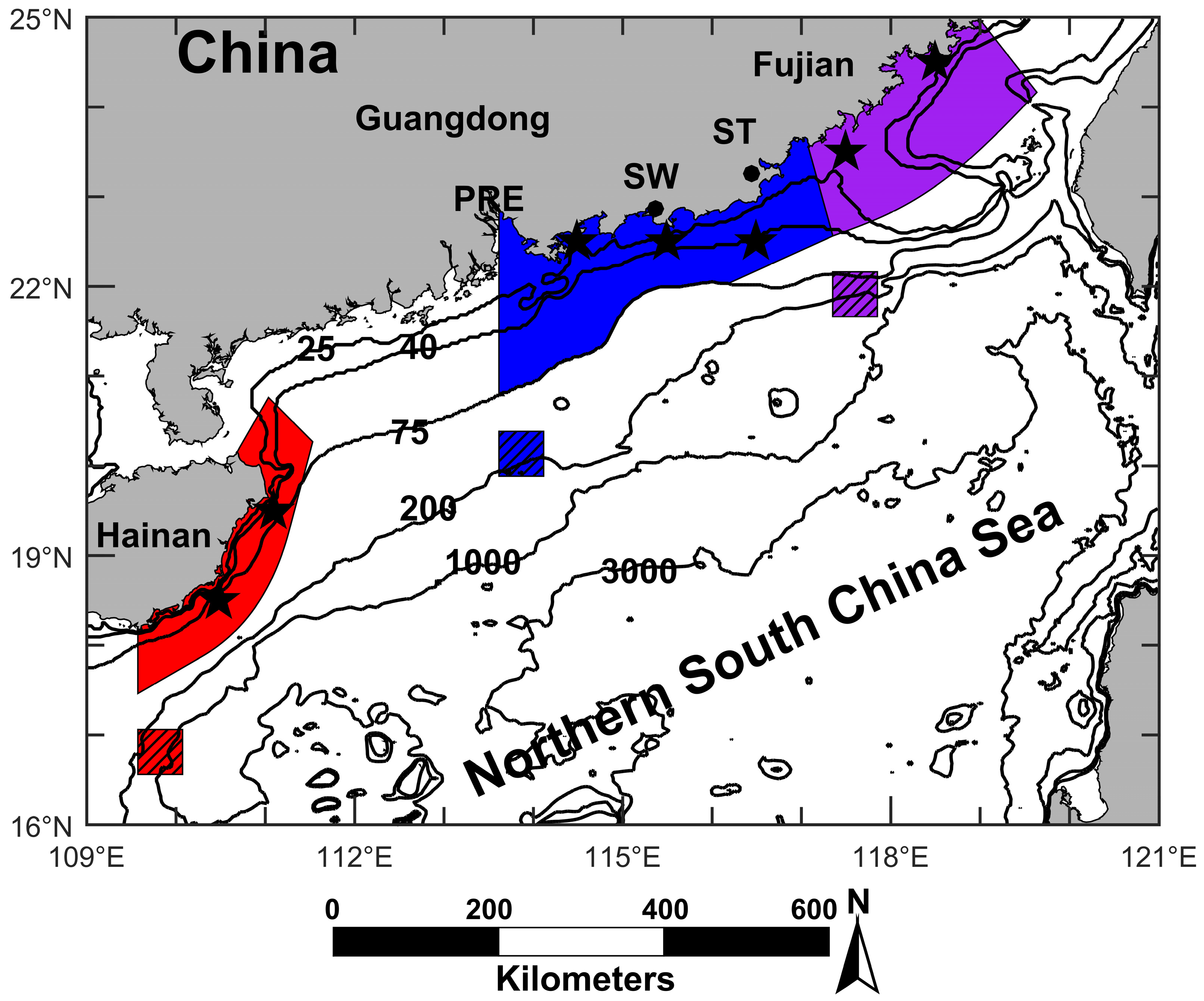
2.1. Study Area
2.2. Himawari-8 Data
2.3. CFSv2 Wind Field Data
2.4. Mapping the Upwelling Area
2.5. Upwelling Index and Wind Stress Curl Calculation Method
2.6. Statistical Analysis
3. Results
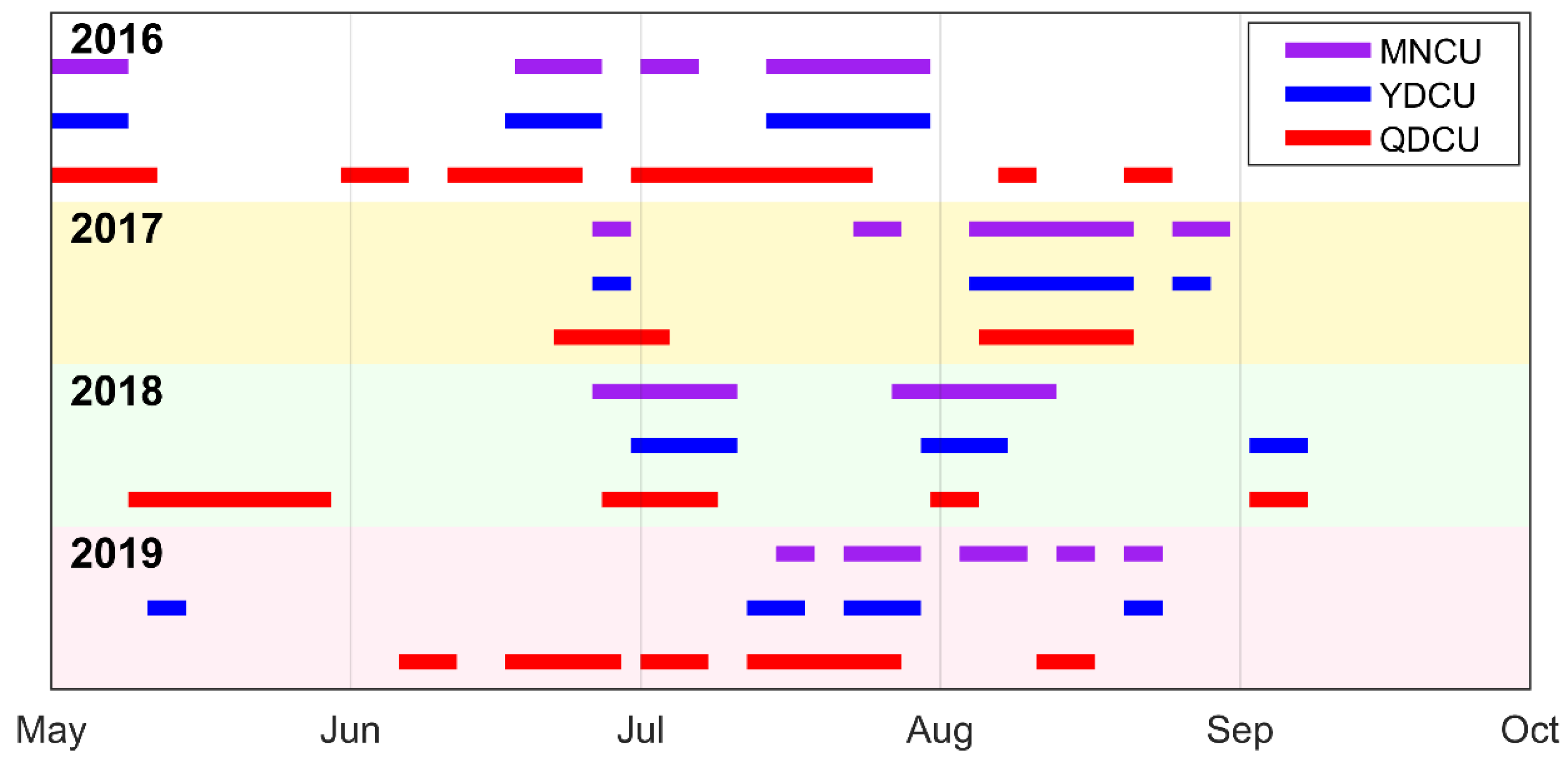
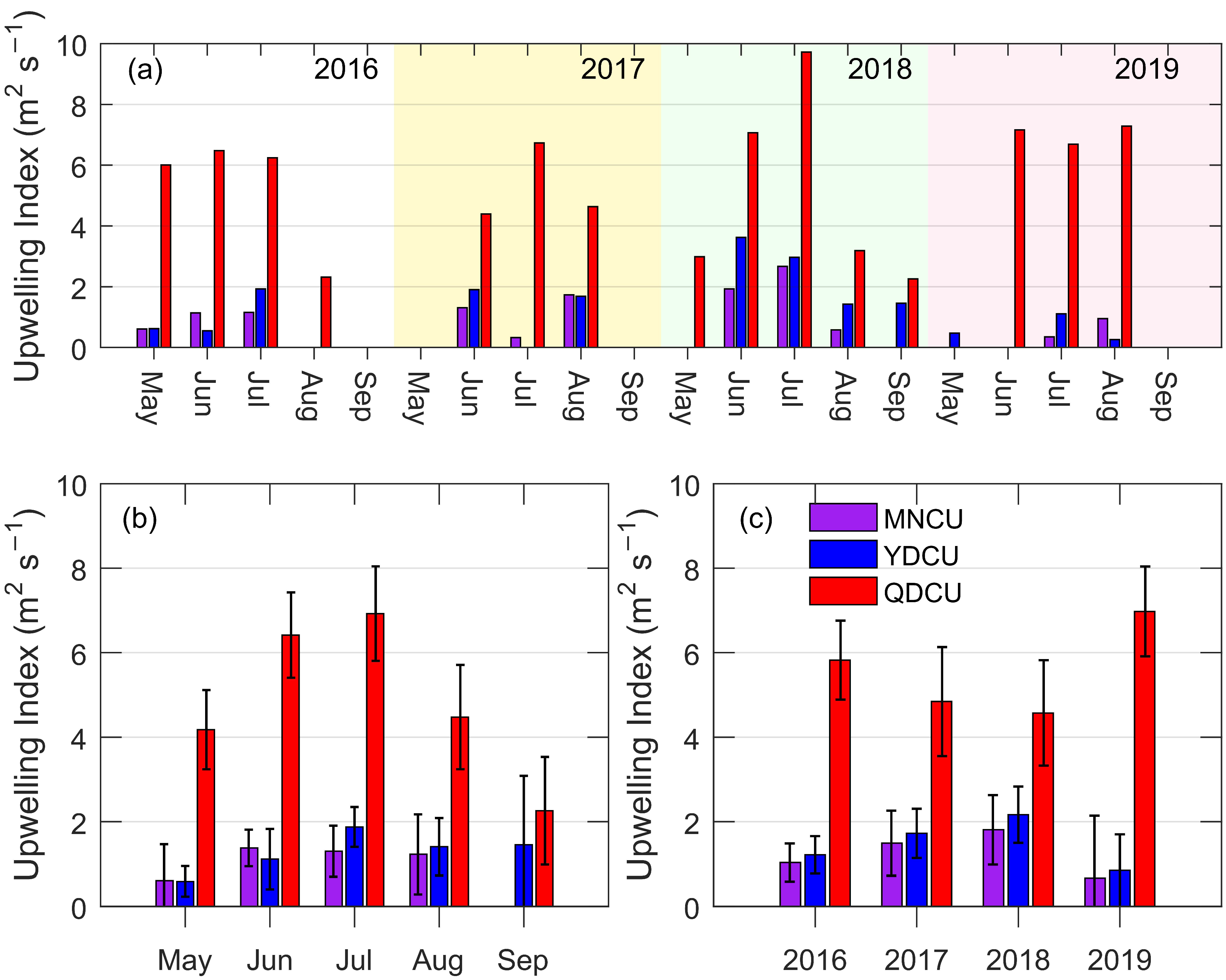
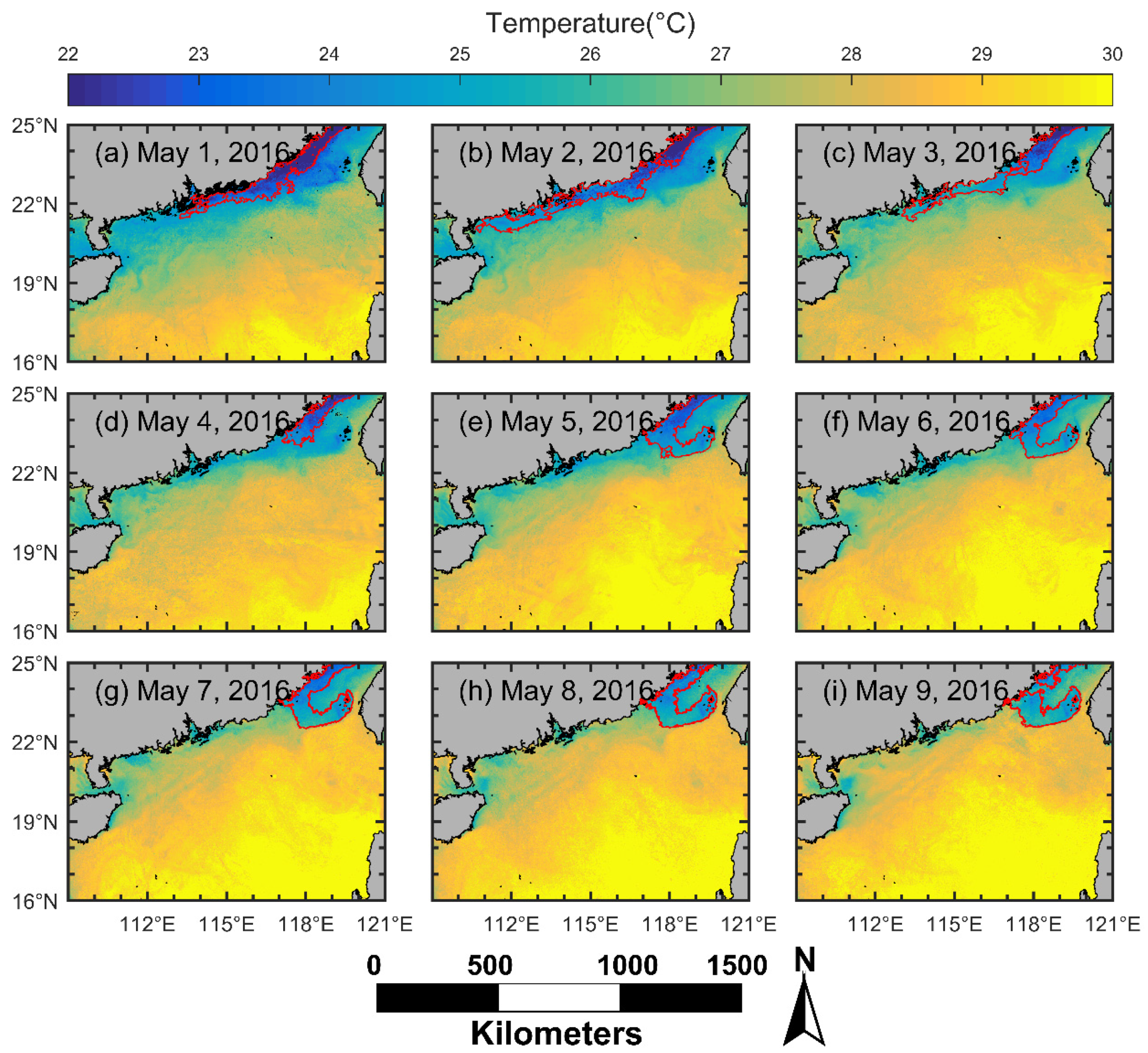
3.1. Upwelling Events
3.2. Spatial Variation of Coastal Upwelling in the NSCS
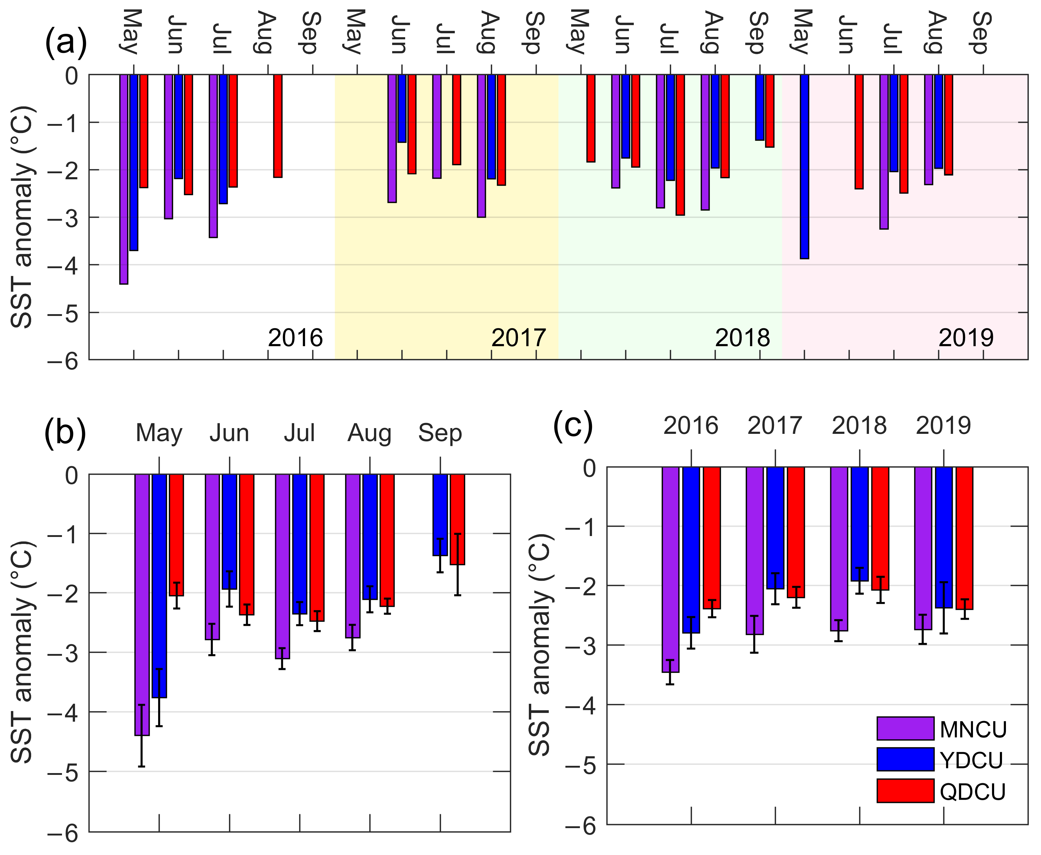
3.3. Variation of Upwelling SST Anomaly in the NSCS
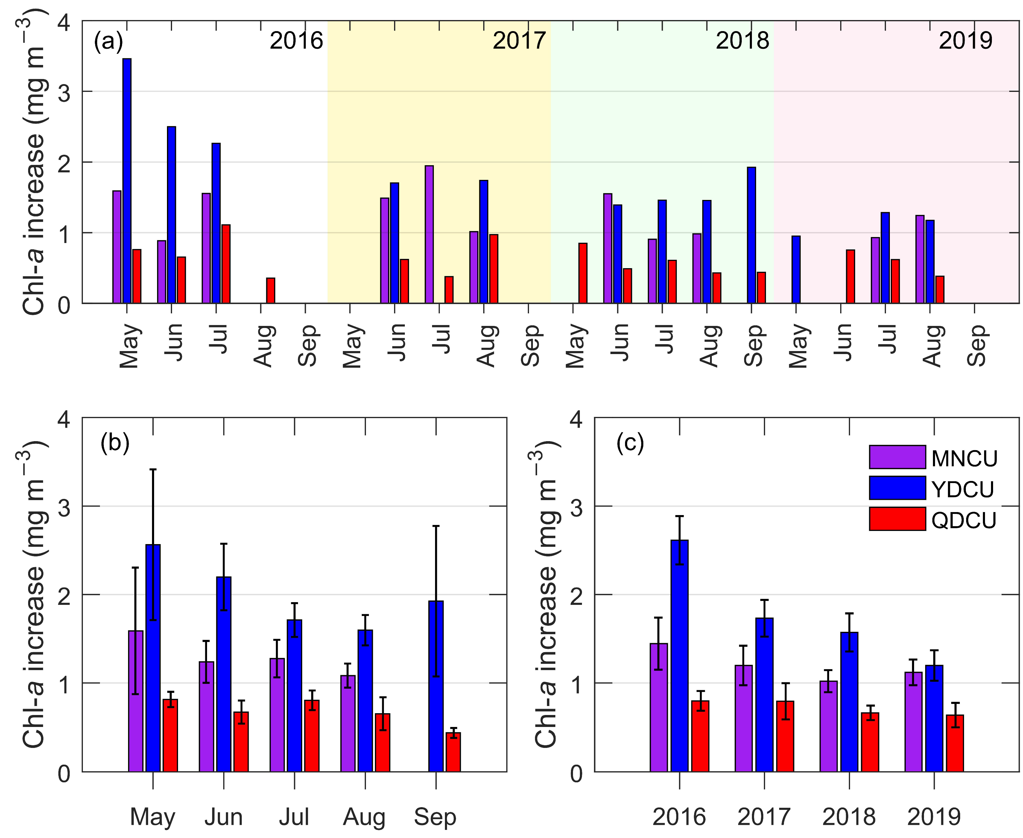
3.4. The Chl-a Increase of the Coastal Upwelling in the NSCS
4. Discussion
4.1. Upwelling Index and Upwelling Mechanisms in the NSCS
4.2. Upwelling Characteristics
5. Conclusions
- (1)
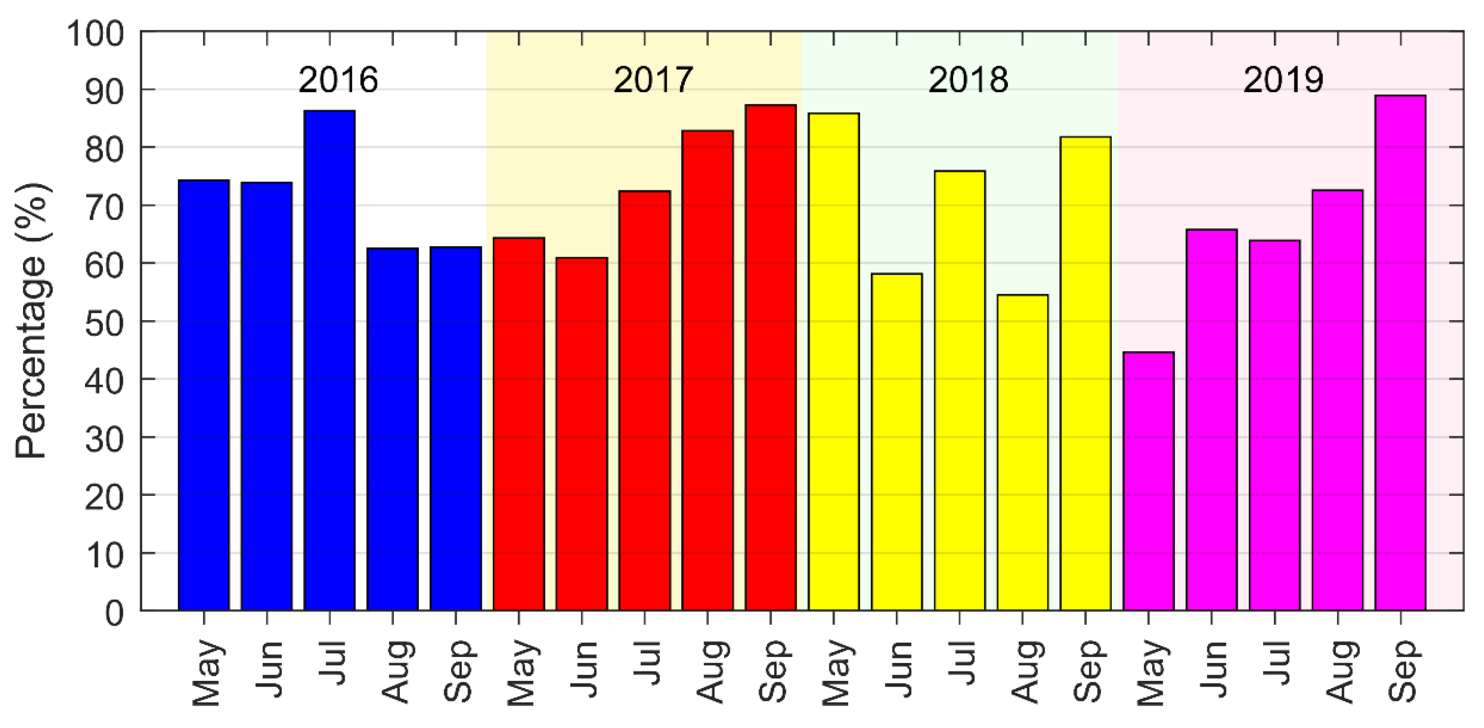
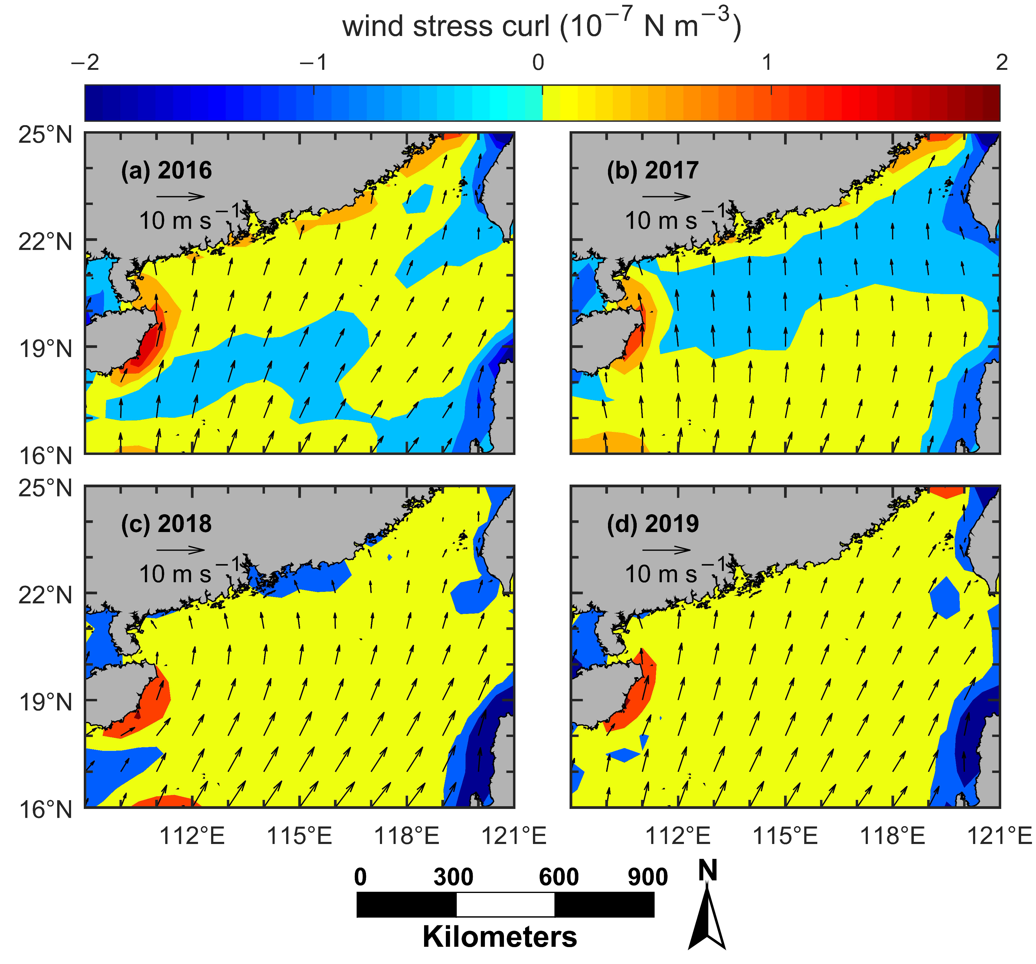
- Based on the Himawari-8 SST data, we have used the semi-automatic TPI based method to identify and map the significant coastal upwelling events and quantitatively analyze the characteristics of coastal upwelling in the NSCS. In general, the strength of the coastal upwelling in the NSCS increased from May, reached the maximum in July, and then decreased to its minimum in September during the boreal summers of 2016–2019. One notable exception to this general pattern is that the upwelling that occurred in May 2016 had unusually large upwelling strength in the Minnan and the Yuedong coastal upwelling regions. In addition, the upwelling strength was much stronger in 2016 than that in next three years, which may be due to the ENSO (El Niño-Southern Oscillation) effect.
- (2)
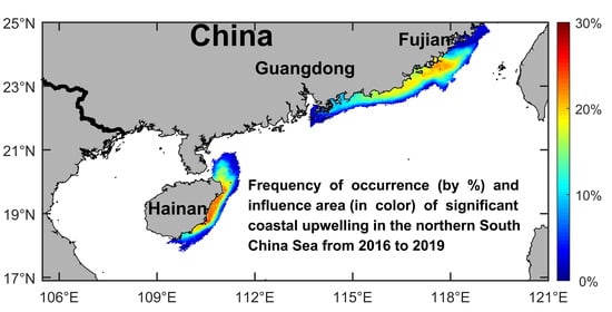
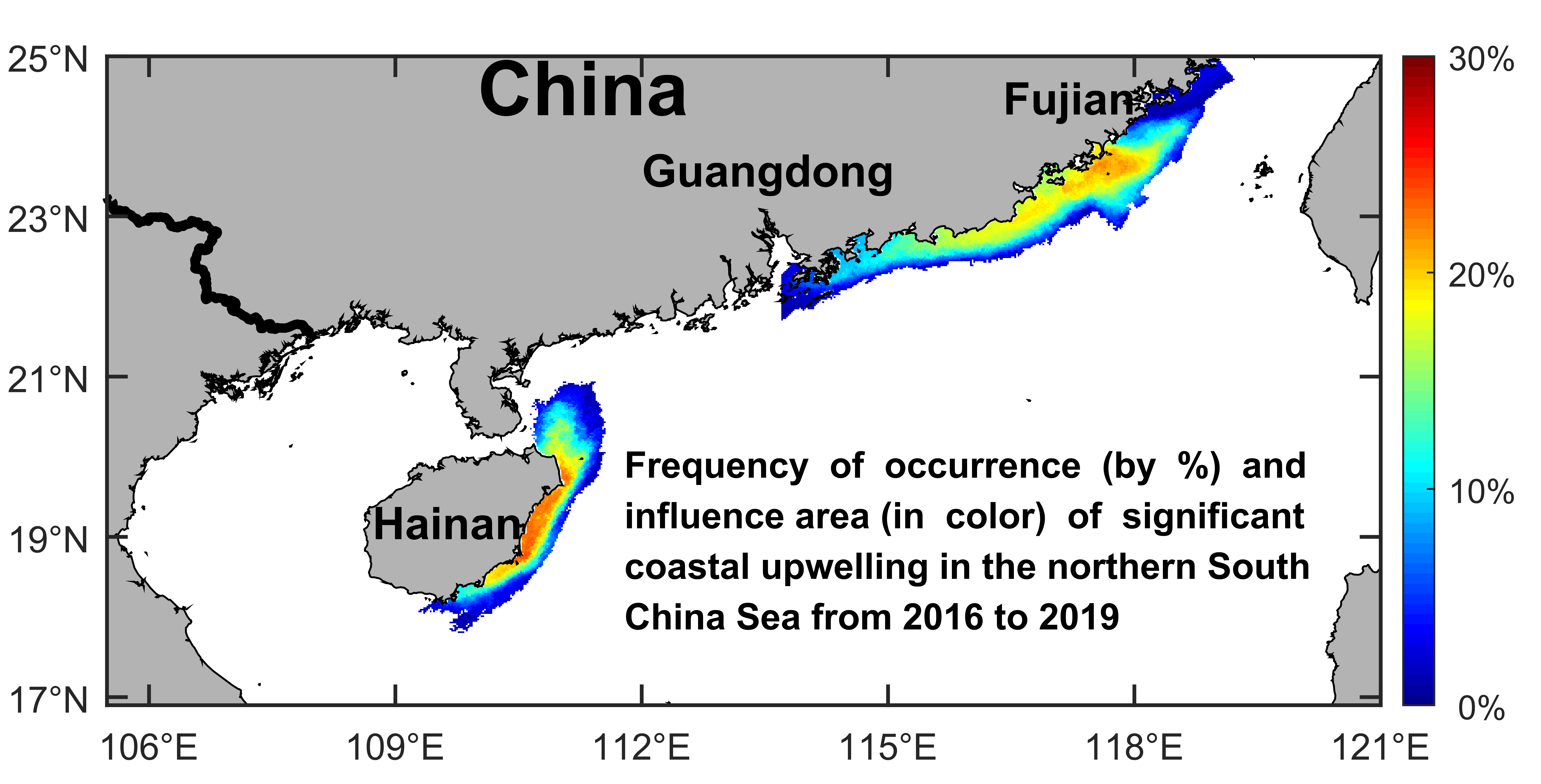
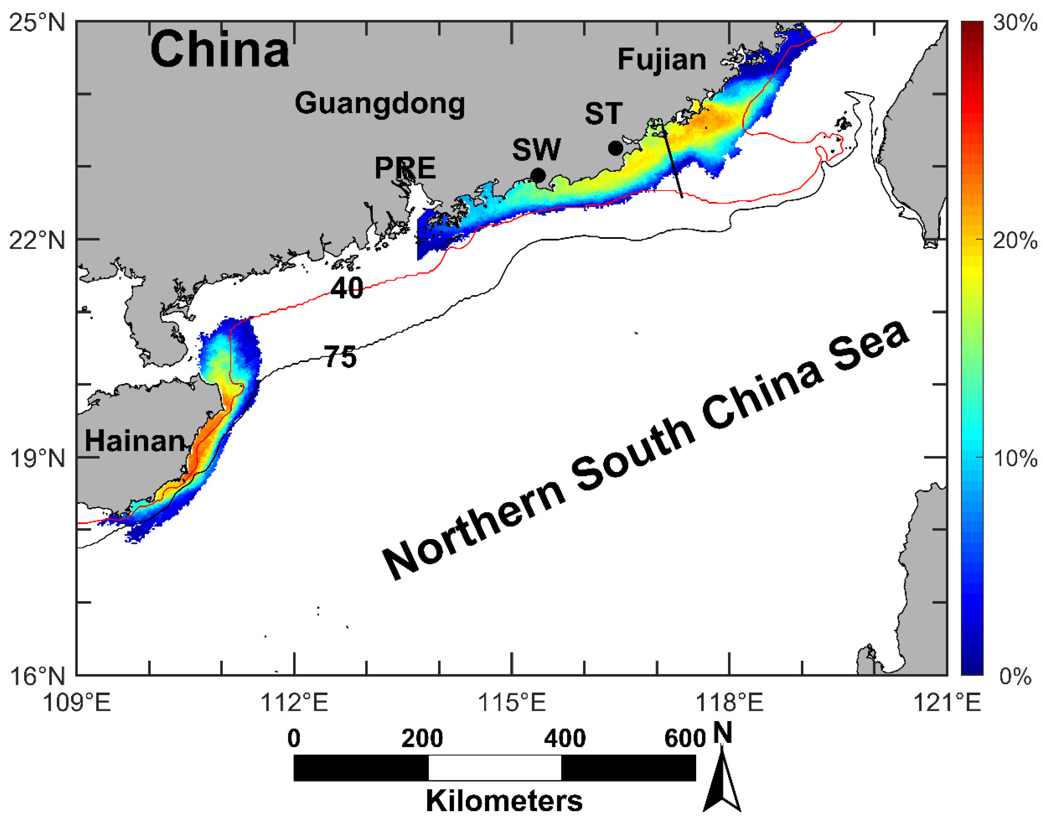
- The area in which upwelling occurs most frequently in the NSCS was specified. The Qiongdong coastal upwelling occurs most frequently off the east coast of Hainan Island, and it is limited to the area shallower than 75 m. The Yuedong coastal upwelling occurs most frequently east of Shanwei, and it is limited to the ≈80 km offshore area within the 40 m depth contour. The Minnan coastal upwelling occurs most frequently off the south coast of Fujian, and it is limited to the ≈100 km offshore area.
- (3)
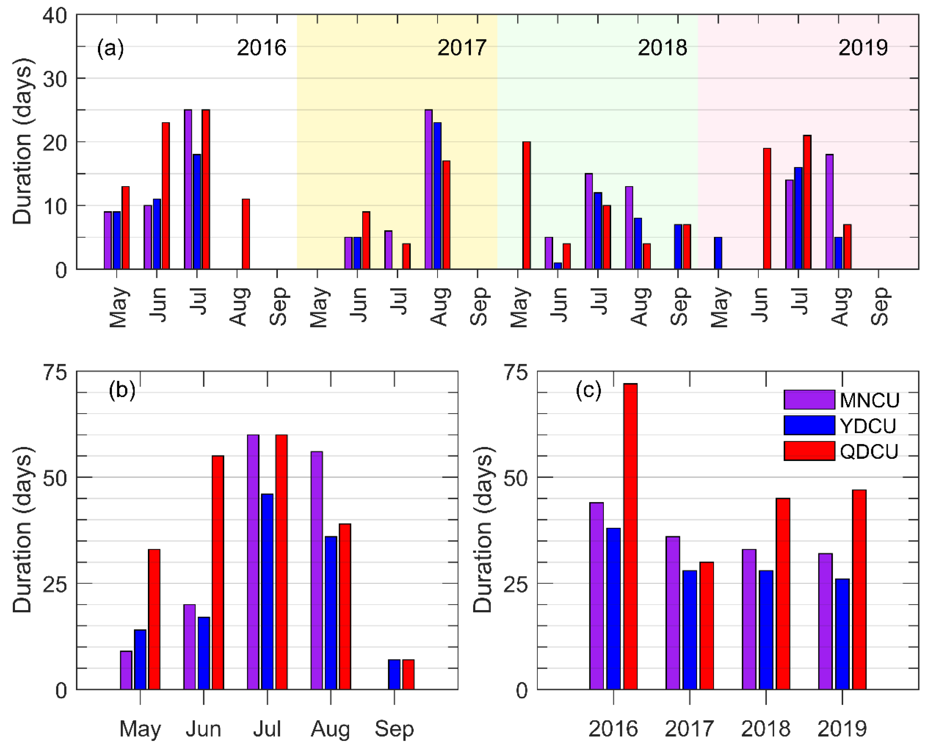
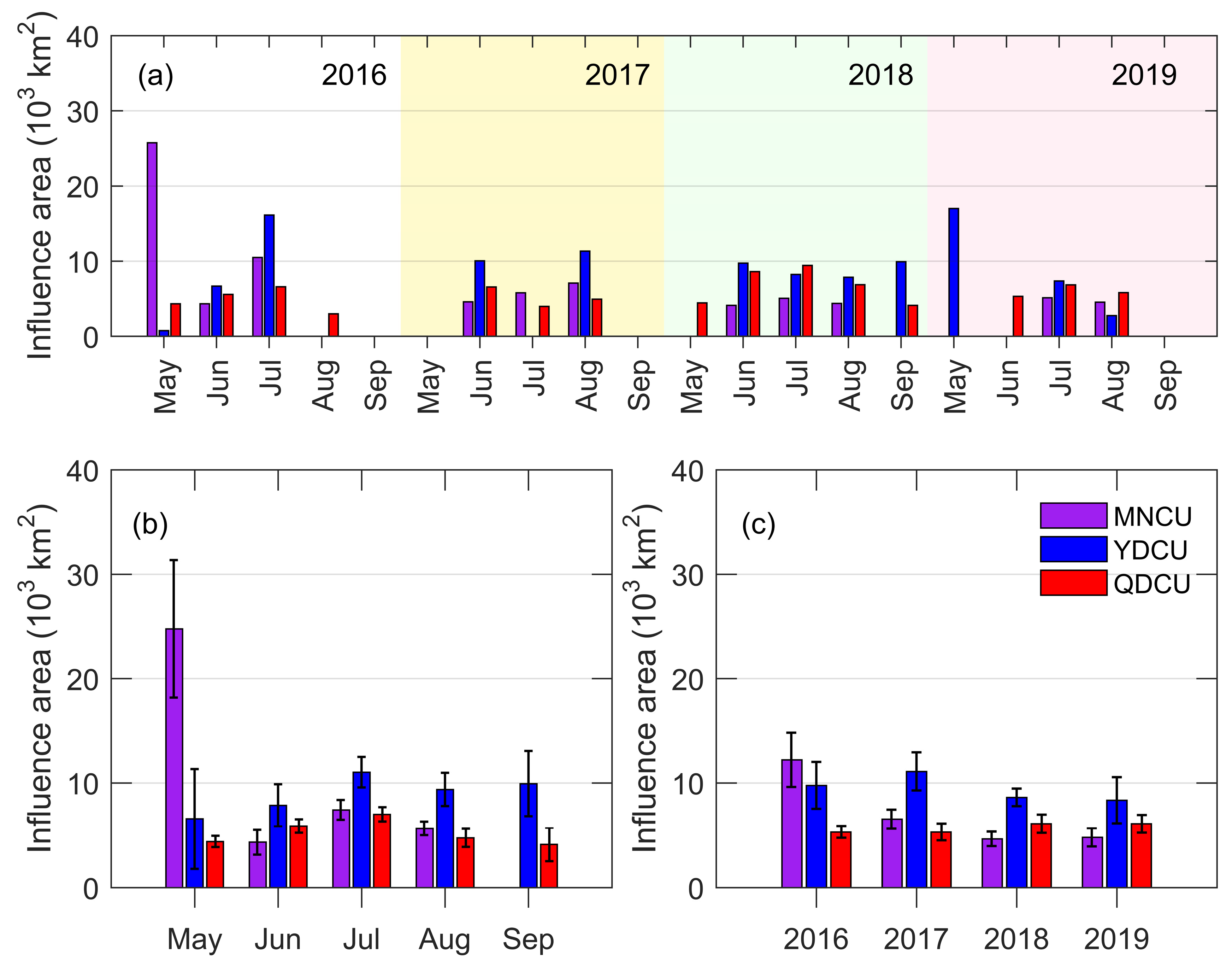
- Different coastal upwelling regions in the NSCS are significantly different in characteristics. Mainly driven by the summer monsoon, the Qiongdong coastal upwelling had the longest duration and occurred most frequently during 2016–2019. As a result of the long coastline, the influence area of the Yuedong coastal upwelling is the largest in the NSCS. In addition, affected by the Pearl River diluted water, the Chl-a increase of the Yuedong coastal upwelling is much larger than that of the other two upwelling regions. In terms of upwelling strength, the Minnan coastal upwelling is quite strong in the NSCS.
- (4)
- The Minnan coastal upwelling and the Yuedong coastal upwelling share many characteristics in common. Especially, their formation mechanisms and temporal variability are similar. Due to the consistence of occurrence time and spatial connection of these two upwellings, it is difficult to distinguish them from one another only by using the SST data.
Author Contributions
Funding
Data Availability Statement
Acknowledgments
Conflicts of Interest
References
- Hu, J.Y.; Kawamura, H.; Hong, H.S.; Qi, Y.Q. A review on the currents in the South China Sea: Seasonal circulation, South China Sea warm current and Kuroshio intrusion. J. Oceanogr. 2000, 56, 607–624. [Google Scholar] [CrossRef]
- Wu, R.S.; Li, L. Summarization of study on upwelling system in the South China Sea. J. Oceangor. Taiwan Strait 2003, 22, 269–276. [Google Scholar]
- Hu, J.Y.; Wang, X.H. Progress on upwelling studies in the China seas. Rev. Geophys. 2016, 54, 653–673. [Google Scholar] [CrossRef]
- Xie, L.L.; Zong, X.L.; Yin, X.F.; Li, M. The interannual variation and long term trend of Qiongdong Upwelling. Oceanol. Limnol. Sin. 2016, 47, 43–51, (In Chinese with English Abstract). [Google Scholar]
- Kok, P.H.; Mohd Akhir, M.F.; Tangang, F.; Husain, M.L. Spatiotemporal trends in the southwest monsoon wind-driven upwelling in the southwestern part of the South China Sea. PLoS ONE 2017, 12, e0171979. [Google Scholar] [CrossRef] [PubMed]
- Shu, Y.Q.; Wang, D.X.; Feng, M.; Geng, B.X.; Chen, J.; Yao, J.L.; Xie, Q.; Liu, Q.Y. The contribution of local wind and ocean circulation to the interannual variability in coastal upwelling intensity in the northern South China Sea. J. Geophys. Res. Oceans. 2018, 123, 6766–6778. [Google Scholar] [CrossRef]
- Li, K.; Gao, L.; Dong, X.; Pan, A.J.; Wang, W.B.; Wan, X.F. The interannual variation and preliminary analysis of upwelling in eastern Hainan Island in summer of 2014 and 2015. Haiyang Xuebao 2019, 41, 1–10, (In Chinese with English Abstract). [Google Scholar]
- Wang, Y.L.; Wu, C.R. Nonstationary El Niño teleconnection on the post-summer upwelling off Vietnam. Sci. Rep. 2020, 10, 13319. [Google Scholar] [CrossRef] [PubMed]
- Ndah, A.B.; Becek, K.; Dagar, L. A review of coastal upwelling research in the South China Sea: Challenges, limitations and prospects. Int. J. Earth Atmos. Sci. 2016, 3, 63–72. [Google Scholar]
- Jing, Z.Y.; Qi, Y.Q.; Hua, Z.L. Numerical study on upwelling and its seasonal variation along Fujian and Zhejiang coast. J. Hohai Univ. 2007, 34, 464–470, (In Chinese with English Abstract). [Google Scholar]
- Wu, L.X.; Lin, H.Y. Preliminary analysis for the summer upwelling in the continental shelf margin waters of east Guangdong. J. Trop. Oceanogr. 1990, 9, 16–23, (In Chinese with English Abstract). [Google Scholar]
- Jing, Z.Y.; Qi, Y.Q.; Yan, D.; Zhang, S.W.; Xie, L.L. Summer upwelling and thermal fronts in the northwestern South China Sea: Observational analysis of two mesoscale mapping surveys. J. Geophys. Res. Oceans. 2015, 120, 1993–2006. [Google Scholar] [CrossRef]
- Bessho, K.; Date, K.; Hayashi, M.; Ikeda, A.; Imai, T.; Inoue, H.; Kumagai, Y.; Miyakawa, T.; Murata, H.; Ohno, T.; et al. An introduction of Himawari-8/9—Japan’s new-generation geostationary meteorological satelites. J. Meteorol. Soc. Japan. 2016, 94, 151–183. [Google Scholar] [CrossRef] [Green Version]
- Kurihara, Y.; Murakami, H.; Kachi, M. Sea surface temperature from the new Japanese geostationary meteorological Himawari-8 satellite. Geophys. Res. Lett. 2016, 43, 1234–1240. [Google Scholar] [CrossRef] [Green Version]
- Murakami, H. Ocean color estimation by Himawari-8/AHI. In Proceedings of the SPIE 9878, Remote Sensing of the Oceans and Inland Waters: Techniques, Applications, and Challenges, New Delhi, India, 4–7 April 2016; Curran Associates, Inc.: Red Hook, NY, USA, 2016; p. 987810. [Google Scholar]
- Sasa, S.; Moorthi, S.; Wu, X.R.; Wang, J.D.; Nadiga, S.; Tripp, P.; Behringer, D.; Hou, Y.T.; Chuang, H.Y.; Iredell, M.; et al. The NECP climate forecast system version2. J. Clim. 2014, 27, 2185–2208. [Google Scholar]
- Weiss, A.D. Topographic Position and Landforms Analysis. In Proceedings of the ESRI International User Conference, San Diego, CA, USA, 9–13 July 2001. [Google Scholar]
- Huang, Z.; Feng, M. Remotely sensed spatial and temporal variability of the Leeuwin Current using MODIS data. Remote Sens. Environ. 2015, 166, 214–232. [Google Scholar] [CrossRef]
- Xie, S.; Huang, Z.; Wang, X. Quantitative mapping of the East Australian Current encroachment using time series Himawari-8 sea surface temperature data. J. Geophys. Res. Ocean. 2020, 125, e2019JC015647. [Google Scholar] [CrossRef]
- Huang, Z.; Wang, X.H. Mapping the spatial and temporal variability of the upwelling systems of the Australian south-eastern coast using 14-year of MODIS data. Remote Sens. Environ. 2019, 227, 90–109. [Google Scholar] [CrossRef]
- Huang, Z.; Hu, J.Y.; Shi, W.S. Mapping the coastal upwelling east of Taiwan using geostationary satellite data. Remote Sens. 2021, 13, 170. [Google Scholar] [CrossRef]
- Jing, Z.Y.; Qi, Y.Q.; Hua, Z.L. Numerical study on summer upwelling over northern continental shelf of South China Sea. J. Trop. Oceanogr. 2008, 3, 1–8, (In Chinese with English Abstract). [Google Scholar]
- Bakun, A. Coastal Upwelling Indices, West Coast of North America, 1946–1971, NOM Tech. Rep. NMFS SSRF-671; Scientific Publications Office: Seattle, WA, USA, 1973; pp. 1–13.
- Wang, D.W.; Gouhier, T.C.; Menge, B.A.; Ganguly, A.R. Intensification and spatial homogenization of coastal upwelling under climate change. Nature 2015, 518, 390–394. [Google Scholar] [CrossRef]
- Kampf, J.; Doubell, M.; Griffin, D.; Matthews, R.L.; Ward, T.M. Evidence of a large seasonal coastal upwelling system along the southern shelf of Australia. Geophys. Res. Lett. 2004, 31, L09310. [Google Scholar] [CrossRef] [Green Version]
- Varela, R.; Alvarez, I.; Santos, F.; de Castro, M.; Gomez-Gesteira, M. Has upwelling strengthened along worldwide coasts over 1982–2010? Sci. Rep. 2015, 5, 10016. [Google Scholar] [CrossRef] [PubMed]
- Wang, D.K.; Wang, H.; Li, M.; Liu, G.M.; Wu, X.Y. Role of Ekman transport versus Ekman pumping in driving summer upwelling in the South China Sea. J. Ocean. Univ. China 2013, 12, 355–365. [Google Scholar] [CrossRef]
- Toba, Y.; Iida, N.; Kawamura, H.; Ebuchi, N.; Jones, I.S.F. Wave dependence of sea-surface wind stress. J. Phys. Oceanogr. 1990, 20, 705–721. [Google Scholar] [CrossRef]
- Gan, J.P.; Cheung, A.; Guo, X.G.; Li, L. Intensified upwelling over a widened shelf in the northeastern South China Sea. J. Geophys. Res. 2009, 114, C09019. [Google Scholar] [CrossRef]
- Wang, D.X.; Shu, Y.Q.; Xue, H.J.; Hu, J.Y.; Chen, J.; Zhuang, W.; Zu, T.T.; Xu, J.D. Relative contributions of local wind and topography to the coastal upwelling intensity in the northern South China Sea. J. Geophys. Res. Oceans. 2014, 119, 2550–2567. [Google Scholar] [CrossRef]
- Cai, S.Z.; Wu, R.S.; Xu, J.D. Characteristics of upwelling in eastern Guangdong and southern Fujian coastal waters during 2006 summer. J. Oceanogr. Taiwan Strait 2011, 30, 489–497, (In Chinese with English Abstract). [Google Scholar]
- Wang, Y.; Jing, Z.Y.; Qi, Y.Q. Coastal upwelling off eastern Hainan Island observed in the summer of 2013. J. Trop. Oceanogr. 2016, 35, 40–49, (In Chinese with English Abstract). [Google Scholar]
- Xie, S.P.; Xie, Q.; Wang, D.X.; Liu, W.T. Summer upwelling in the South China Sea and its role in regional climate variations. J. Geophys. Res. Oceans. 2003, 108, 3261. [Google Scholar] [CrossRef] [Green Version]
- Han, A.Q.; Dai, M.H.; Kao, S.J.; Gan, J.P.; Li, Q.; Wang, L.F.; Zhai, W.D.; Wang, L. Nutrient dynamics and biological consumption in a large continental shelf system under the influence of both a river plume and coastal upwelling. Limnol. Oceanogr. 2012, 57, 486–502. [Google Scholar] [CrossRef] [Green Version]
- Gan, J.P.; Li, L.; Wang, D.X.; Guo, X.G. Interaction of a river plume with coastal upwelling in the northeastern South China Sea. Cont. Shelf. Res. 2009, 29, 728–740. [Google Scholar] [CrossRef]
- Luo, L.; Zhou, W.; Wang, D. Responses of the river plume to the external forcing in Pearl River Estuary. Aquat. Ecosyst. Health Manag. 2012, 15, 62–69. [Google Scholar] [CrossRef]
- Yang, Y.; Li, R.X.; Zhu, P.L.; Ren, P.D. Seasonal variation of the Pearl River diluted water and its dynamical cause. Marin. Sci. Bull. 2014, 33, 36–44, (In Chinese with English Abstract). [Google Scholar]


| Minnan Coastal Upwelling | Influence Area | SST_A | Chl-a Increase | Upwelling Index |
|---|---|---|---|---|
| Duration | 0.47 * | −0.78 | 0.70 | 0.66 |
| Influence Area | −0.80 | 0.68 | 0.32 * | |
| SST_A | −0.88 | −0.67 | ||
| Chl-a Increase | 0.65 |
| Yuedong Coastal Upwelling | Influence Area | SST_A | Chl-a Increase | Upwelling Index |
|---|---|---|---|---|
| Duration | 0.65 | −0.67 | 0.69 | 0.48 * |
| Influence area | −0.73 | 0.56 | 0.67 | |
| SST_A | −0.84 | −0.48 | ||
| Chl-a Increase | 0.54 |
| Qiongdong Coastal Upwelling | Influence Area | SST_A | Chl-a Increase | Upwelling Index |
|---|---|---|---|---|
| Duration | 0.54 | −0.74 | 0.88 | 0.58 |
| Influence area | −0.89 | 0.72 | 0.88 | |
| SST_A | −0.84 | −0.88 | ||
| Chl-a Increase | 0.69 |
Publisher’s Note: MDPI stays neutral with regard to jurisdictional claims in published maps and institutional affiliations. |
© 2021 by the authors. Licensee MDPI, Basel, Switzerland. This article is an open access article distributed under the terms and conditions of the Creative Commons Attribution (CC BY) license (http://creativecommons.org/licenses/by/4.0/).
Share and Cite
Shi, W.; Huang, Z.; Hu, J. Using TPI to Map Spatial and Temporal Variations of Significant Coastal Upwelling in the Northern South China Sea. Remote Sens. 2021, 13, 1065. https://doi.org/10.3390/rs13061065
Shi W, Huang Z, Hu J. Using TPI to Map Spatial and Temporal Variations of Significant Coastal Upwelling in the Northern South China Sea. Remote Sensing. 2021; 13(6):1065. https://doi.org/10.3390/rs13061065
Chicago/Turabian StyleShi, Weian, Zhi Huang, and Jianyu Hu. 2021. "Using TPI to Map Spatial and Temporal Variations of Significant Coastal Upwelling in the Northern South China Sea" Remote Sensing 13, no. 6: 1065. https://doi.org/10.3390/rs13061065