Inundation Assessment of the 2019 Typhoon Hagibis in Japan Using Multi-Temporal Sentinel-1 Intensity Images


Abstract
:1. Introduction
2. Study Area and Sentinel-1 Imagery
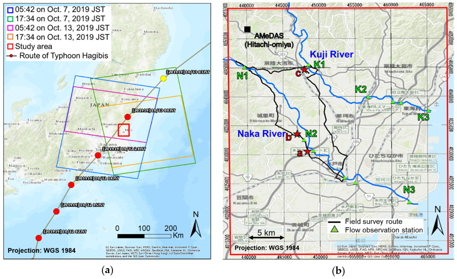
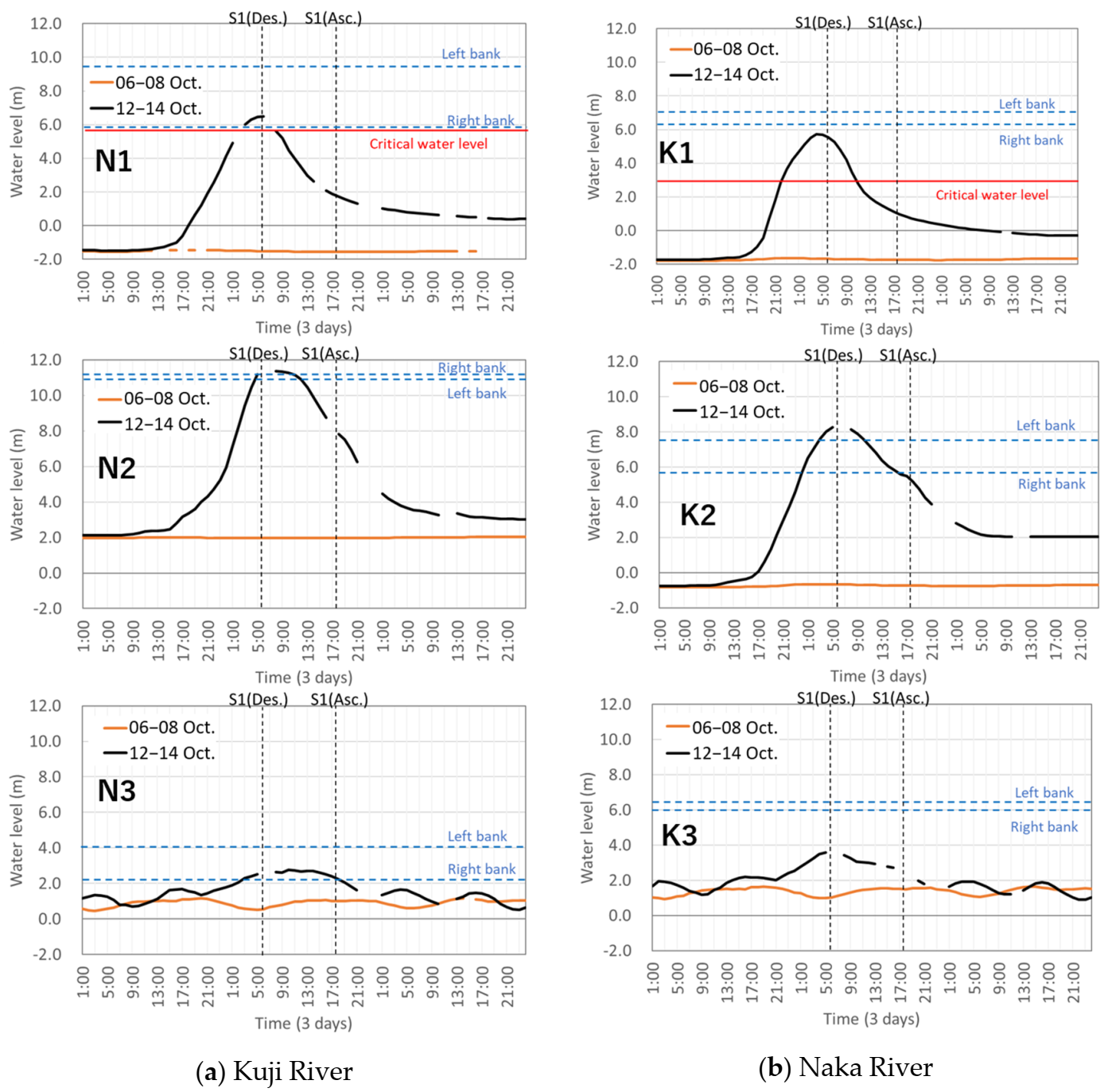
2.1. Study Area of Ibaraki Prefurcture, Japan
2.2. Sentinel-1 Images and Pre-Processing
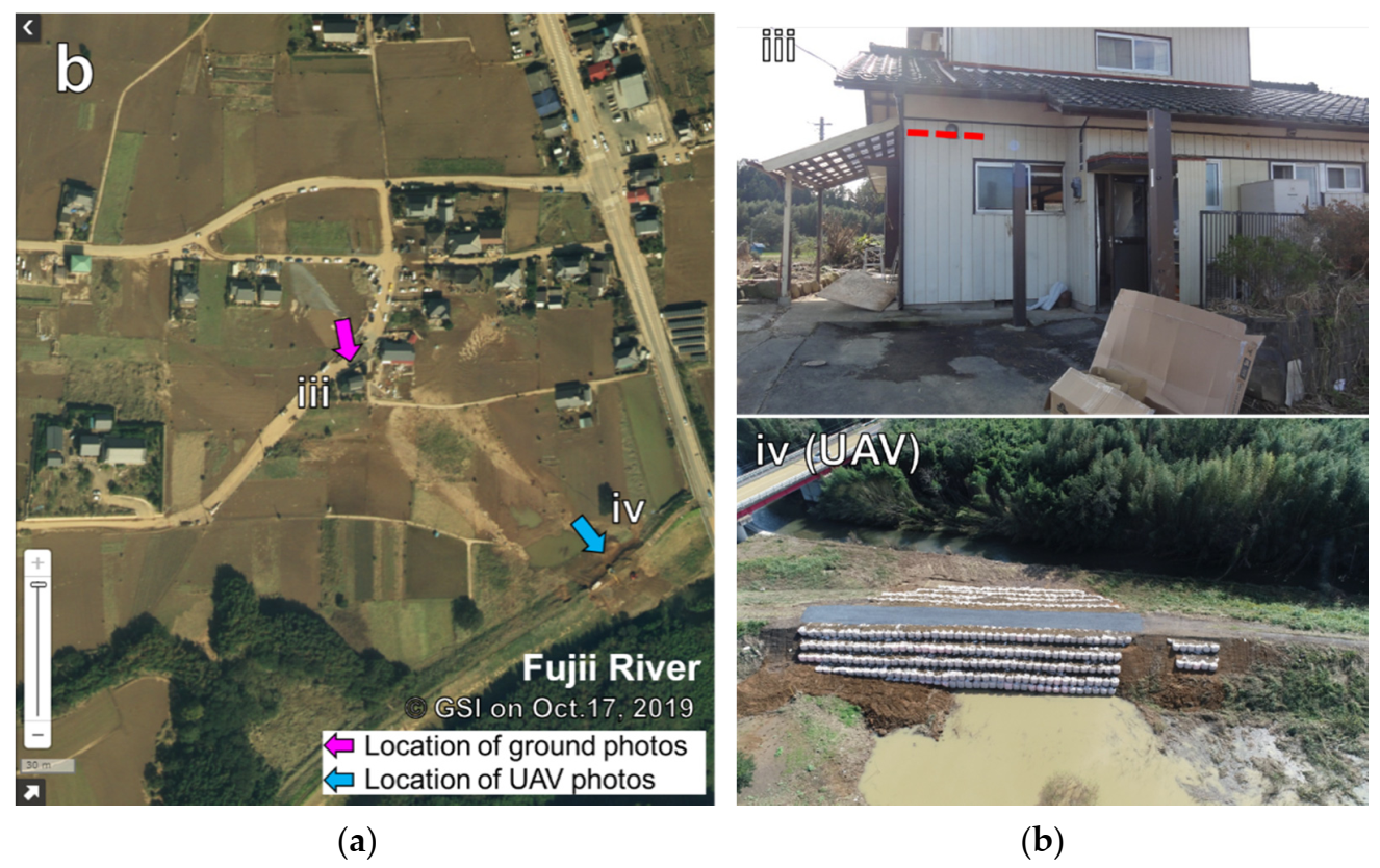
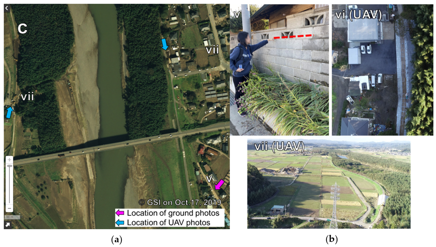
3. The Field Survey
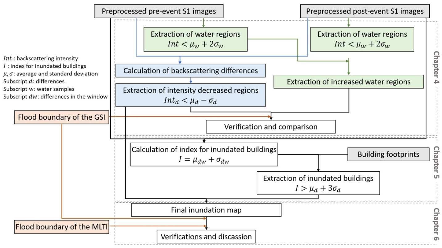
4. Extraction of Completely Inundated Areas
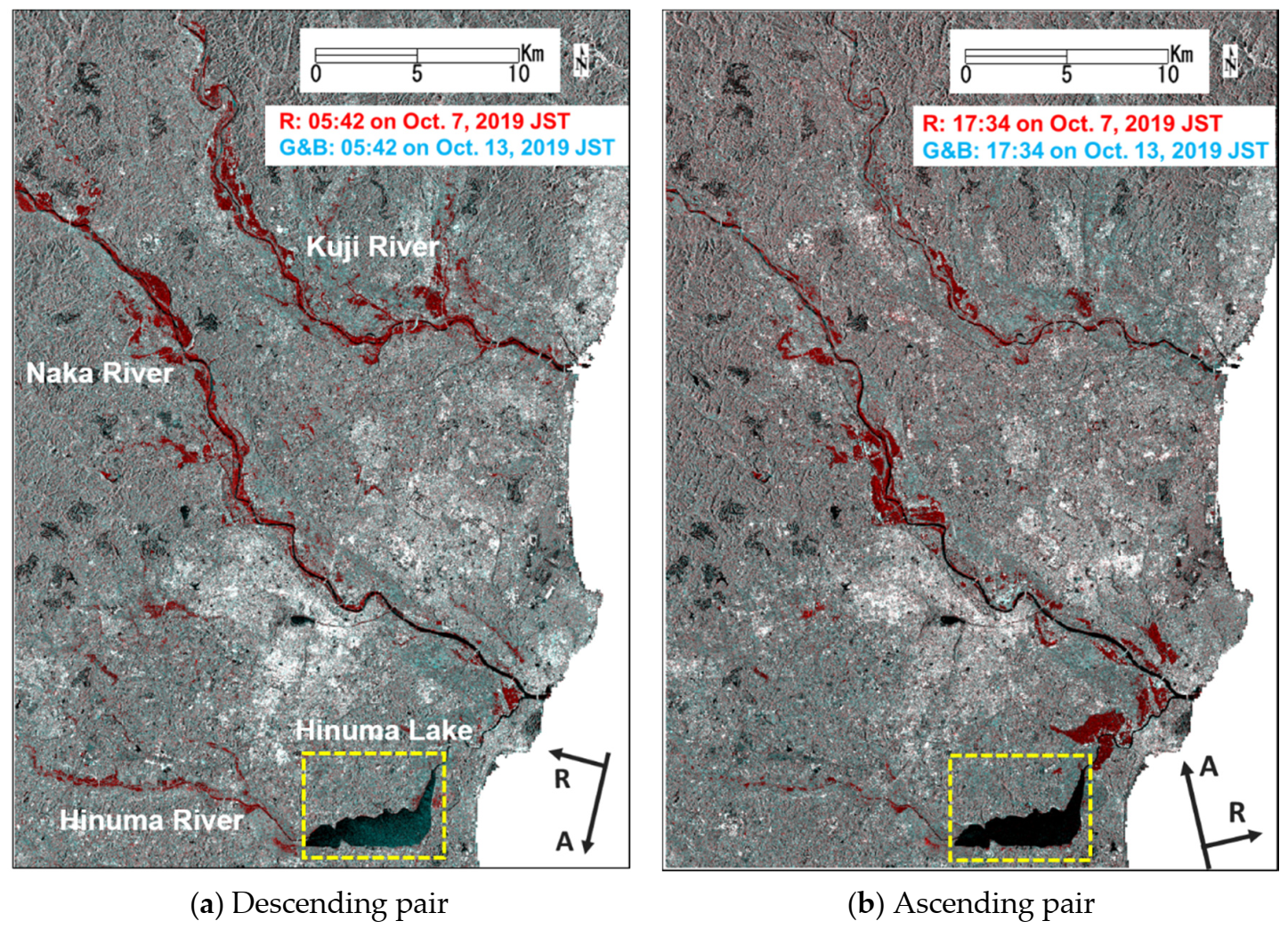
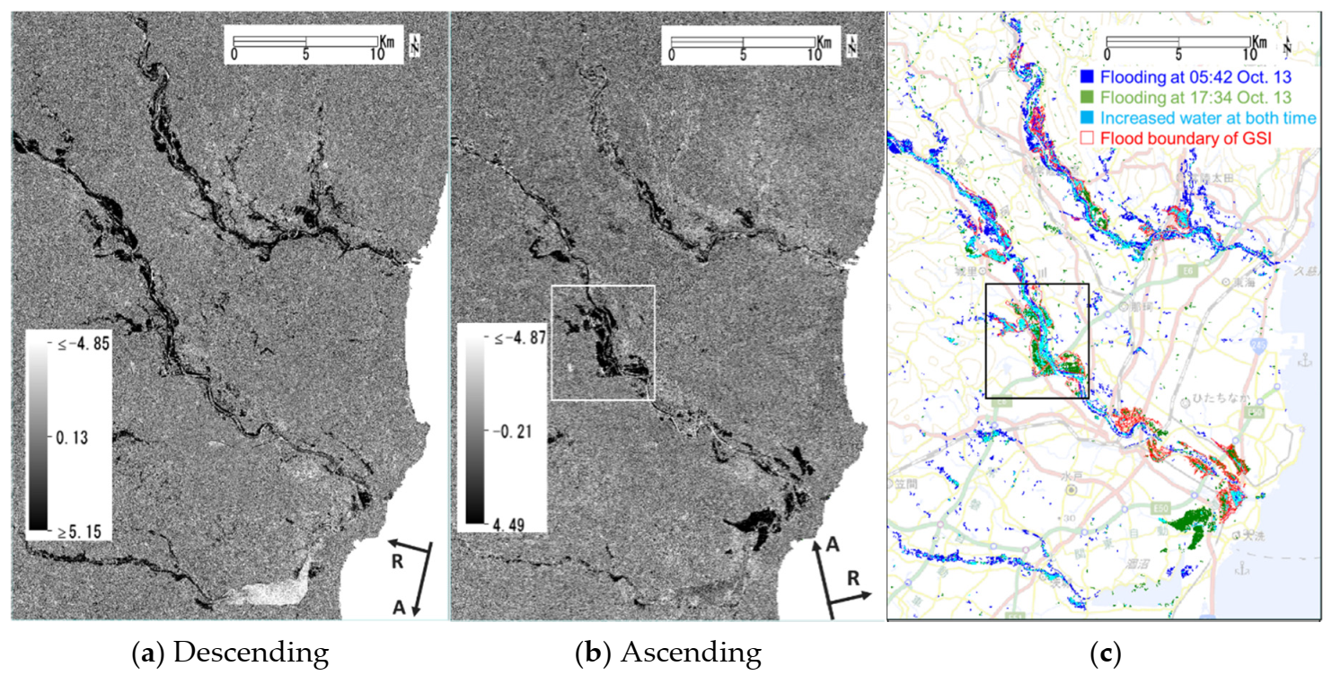
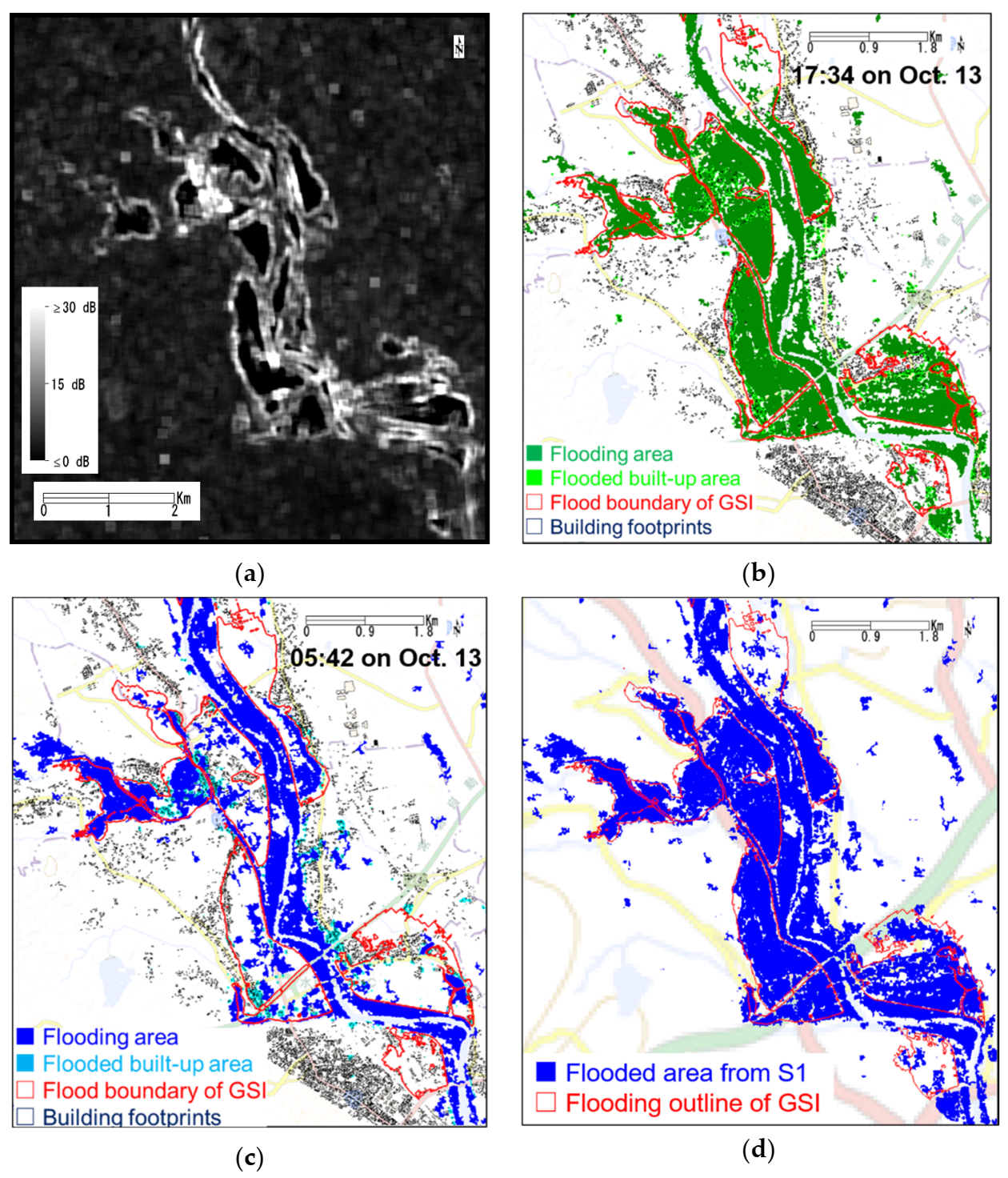
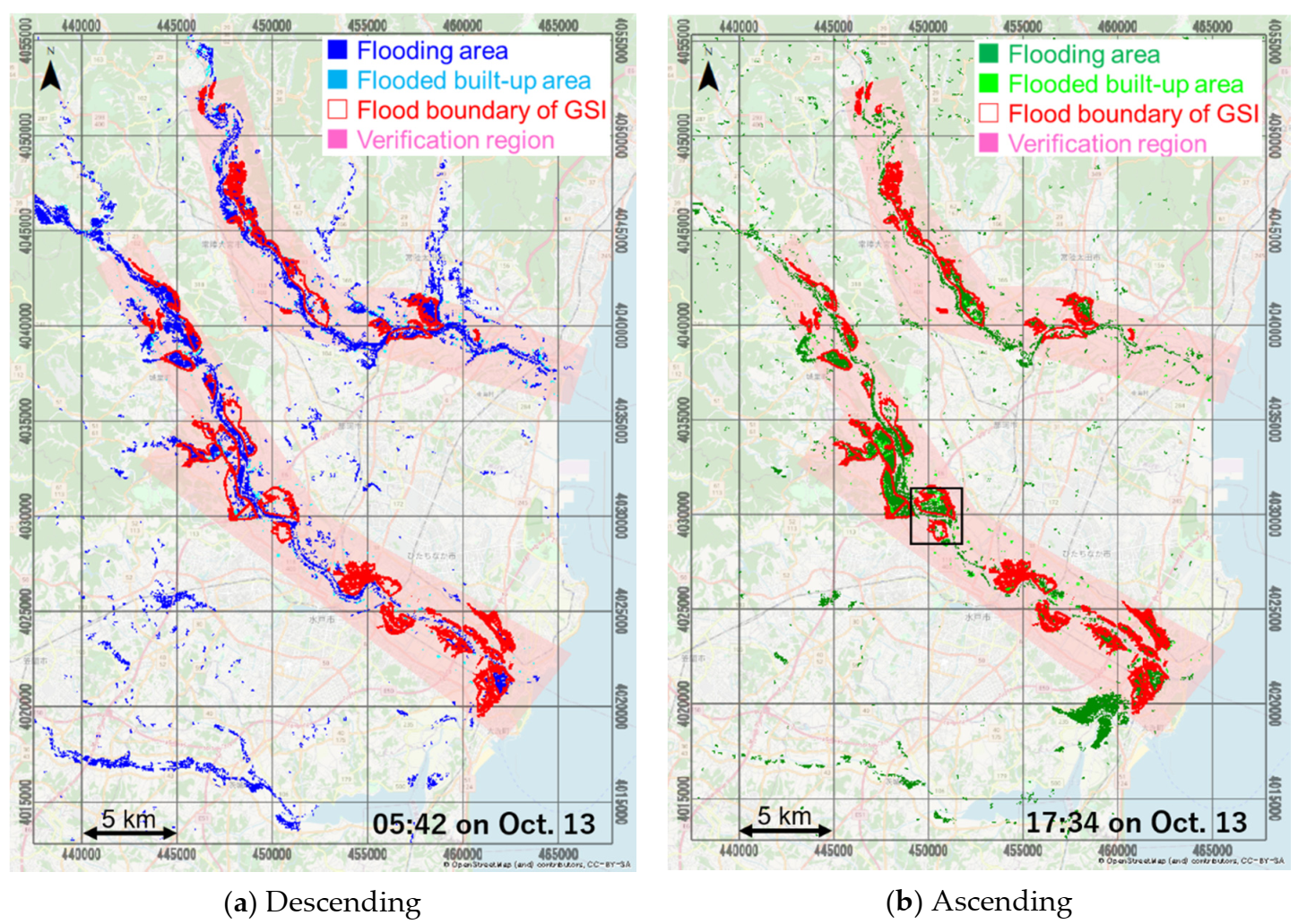
4.1. Multi-Temporal Comparison
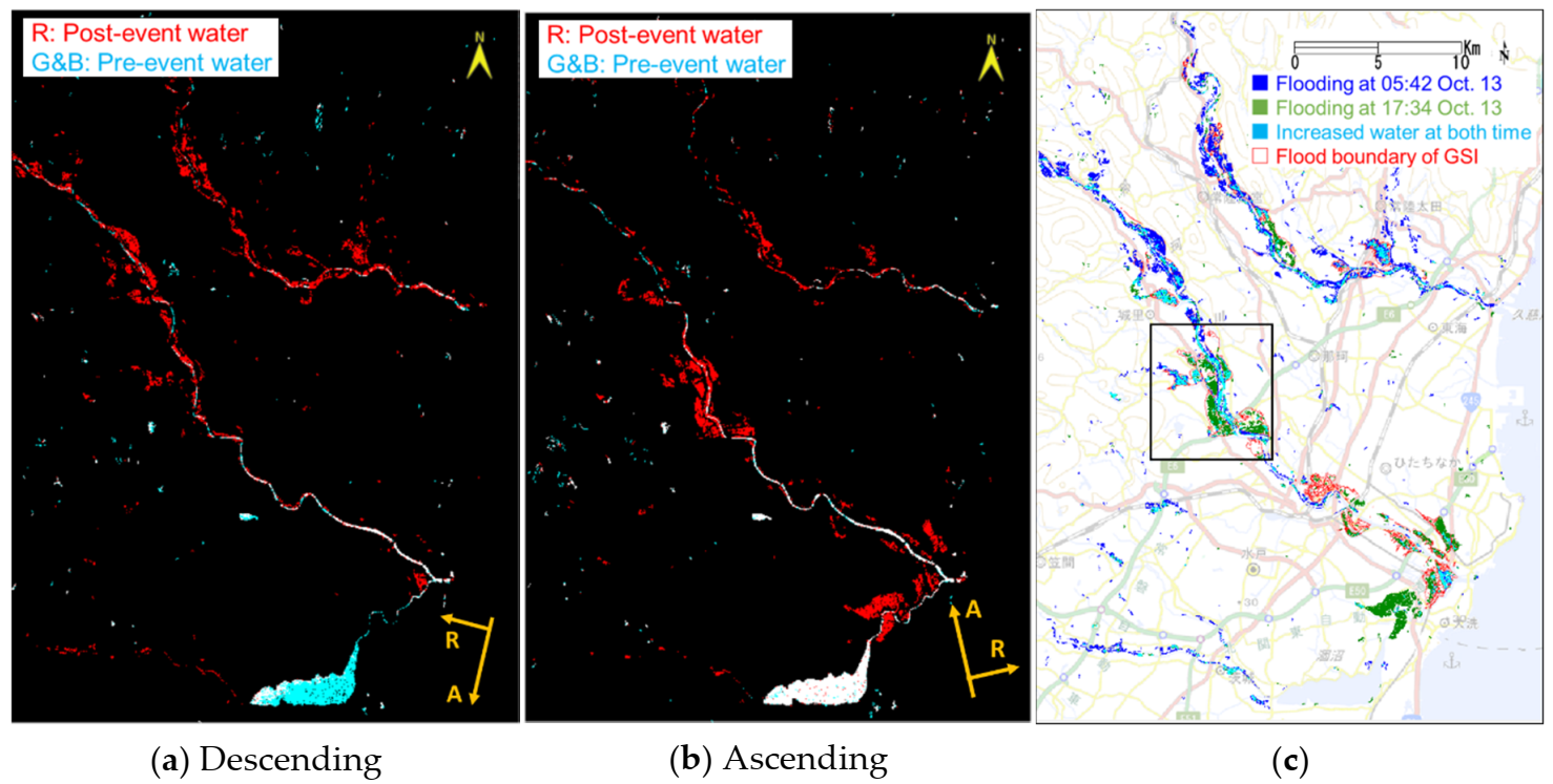
4.2. Mono-Temporal Determination
4.3. Comparison and Verificiation
5. Extraction of the Partly Inundated Built-Up Areas
5.1. Backscatter Model of Partly Inundated Buildings
5.2. Index for Inundated Buildings
5.3. Verfication
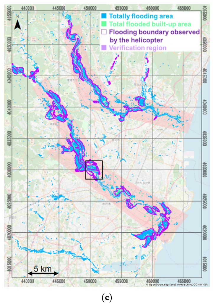
6. Final Inundation Maps and Discussion
6.1. Verfication Using the GSI’s Boundary
6.2. Verfication Using the MLIT’s Boundary
6.3. Disscusion
7. Conclusions
Author Contributions
Funding
Institutional Review Board Statement
Informed Consent Statement
Data Availability Statement
Acknowledgments
Conflicts of Interest
References
- Centre for Research on the Epidemiology of Disasters—CRED. Natural Disasters 2019: Now Is the Time to Not Give Up. 2020. Available online: https://cred.be/sites/default/files/adsr_2019.pdf (accessed on 20 December 2020).
- Japan Meteorological Agency. Breaking News of the Features and the Factors of the 2020 Typhoon Hagibis. 2019. Available online: https://www.jma.go.jp/jma/press/1910/24a/20191024_mechanism.pdf (accessed on 20 December 2020). (In Japanese)
- Cabinet Office, Government of Japan. Report of the Damage Situation Related to the Typhoon No. 19 (Hagibis) until 09:00 on 10 April 2020. Available online: http://www.bousai.go.jp/updates/r1typhoon19/pdf/r1typhoon19_45.pdf (accessed on 20 December 2020). (In Japanese)
- The International Charter Space and Major Disaster. Typhoon Hagibis in Japan. Available online: https://disasterscharter.org/web/guest/activations/-/article/storm-hurricane-urban-in-japan-activation-625- (accessed on 20 December 2020).
- Dell’Acqua, F.; Gamba, P. Remote sensing and earthquake damage assessment: Experiences, limits, and perspectives. Proc. IEEE 2012, 100, 2876–2890. [Google Scholar] [CrossRef]
- Nakmuenwai, P.; Yamazaki, F.; Liu, W. Multi-temporal correlation method for damage assessment of buildings from high-resolution SAR images of the 2013 Typhoon Haiyan. J. Disaster Res. 2016, 11, 557–592. [Google Scholar] [CrossRef]
- Wieland, M.; Liu, W.; Yamazaki, F. Learning change from Synthetic Aperture Radar images: Performance evaluation of a Support Vector Machine to detect earthquake and tsunami-induced changes. Remote Sens. 2016, 8, 792. [Google Scholar] [CrossRef] [Green Version]
- Nakmuenwai, P.; Yamazaki, F.; Liu, W. Automated extraction of inundated areas from multi-temporal dualpolarization RADARSAT-2 images of the 2011 central Thailand flood. Remote Sens. 2017, 9, 78. [Google Scholar] [CrossRef] [Green Version]
- Karimzadeh, S.; Matsuoka, M. Building damage assessment using multisensor dualpolarized synthetic aperture radar data for the 2016 M 6.2 Amatrice earthquake, Italy. Remote Sens. 2017, 9, 330. [Google Scholar] [CrossRef] [Green Version]
- Fan, Y.; Wen, Q.; Wang, W.; Wang, P.; Li, L.; Zhang, P. Quantifying disaster physical damage using remote sensing data—A technical work flow and case study of the 2014 Ludian earthquake in China. Int. J. Disaster Risk Sci. 2017, 8, 471–492. [Google Scholar] [CrossRef]
- Ferrentino, E.; Marino, A.; Nunziata, F.; Migliaccio, M. A dual-polarimetric approach to earthquake damage assessment. Int. J. Remote Sens. 2019, 40, 197–217. [Google Scholar] [CrossRef]
- Klemas, V. Remote sensing of floods and flood-prone areas: An overview. J. Coast. Res. 2015, 31, 1005–1013. [Google Scholar] [CrossRef]
- Lin, L.; Di, L.; Yu, E.G.; Kang, L.; Shrestha, R.; Rahman, M.S.; Tang, J.; Deng, M.; Sun, Z.; Zhang, C.; et al. A review of remote sensing in flood assessment. In Proceedings of the 2016 Fifth International Conference on Agro-Geoinformatics, Tianjin, China, 18–20 July 2016. [Google Scholar] [CrossRef]
- Koshimura, S.; Moya, L.; Mas, E.; Bai, Y. Tsunami damage detection with remote sensing: A review. Geosciences 2020, 10, 177. [Google Scholar] [CrossRef]
- McFeeters, S.K. The use of the normalized difference water index (NDWI) in the delineation of open water features. Int. J. Remote Sens. 1996, 17, 1425–1432. [Google Scholar] [CrossRef]
- Xu, H. Modification of normalised difference water index (NDWI) to enhance open water features in remotely sensed imagery. Int. J. Remote Sens. 2006, 27, 3025–3033. [Google Scholar] [CrossRef]
- Feyisa, G.L.; Meilby, H.; Fensholt, R.; Proud, S.R. Automated water extraction index: A new technique for surface water mapping using Landsat imagery. Remote Sens. Environ. 2014, 140, 23–35. [Google Scholar] [CrossRef]
- Xie, H.; Luo, X.; Xu, X.; Tong, X.; Jin, Y.; Pan, H.; Zhou, B. New hyperspectral difference water index for the extraction of urban water bodies by the use of airborne hyperspectral images. J. Appl. Remote Sens. 2014, 8, 085098. [Google Scholar] [CrossRef] [Green Version]
- Ko, B.C.; Kim, H.H.; Nam, J.Y. Classification of potential water bodies using Landsat 8 OLI and a combination of two boosted random forest classifiers. Sensors 2015, 15, 13763–13777. [Google Scholar] [CrossRef] [Green Version]
- Ogilvie, A.; Belaud, G.; Delenne, C.; Bailly, J.-S.; Bader, J.-C.; Oleksiak, A.; Ferry, L.; Martin, D. Decadal monitoring of the Niger Inner Delta flood dynamics using MODIS optical data. J. Hydrol. 2015, 523, 368–383. [Google Scholar] [CrossRef] [Green Version]
- Hakkenberg, C.; Dannenberg, M.; Song, C.; Ensor, K. Characterizing multi-decadal, annual land cover change dynamics in Houston, TX based on automated classification of Landsat imagery. Int. J. Remote Sens. 2018, 40, 693–718. [Google Scholar] [CrossRef]
- Nandi, I.; Srivastava, P.K.; Shah, K. Floodplain Mapping through Support Vector Machine and Optical/Infrared Images fromLandsat 8 OLI/TIRS Sensors: Case Study from Varanasi. Water Resour. Manag. 2017, 31, 1157–1171. [Google Scholar] [CrossRef]
- Pulvirenti, L.; Pierdicca, N.; Chini, M.; Guerriero, L. An algorithm for operational flood mapping from Synthetic Aperture Radar (SAR) data using fuzzy logic. Nat. Hazards Earth Syst. Sci. 2011, 11, 529–540. [Google Scholar] [CrossRef] [Green Version]
- Westerhoff, R.S.; Kleuskens, M.P.; Winsemius, H.C.; Huizinga, H.J.; Brakenridge, G.R.; Bishop, C. Automated global water mapping based on wide-swath orbital synthetic-aperture radar. Hydrol. Earth Syst. Sci. 2013, 17, 651–663. [Google Scholar] [CrossRef] [Green Version]
- Liu, W.; Yamazaki, F. Detection of inundation areas due to the 2015 Kanto and Tohoku torrential rain in Japan based on multi-temporal ALOS-2 imagery. Nat. Hazards Earth Syst. Sci. 2018, 18, 1905–1918. [Google Scholar] [CrossRef] [Green Version]
- Martinis, S.; Twele, A.; Voigt, S. Towards operational near real-time flood detection using a split-based automatic thresholding procedure on high resolution TerraSAR-X data. Nat. Hazards Earth Syst. Sci. 2009, 9, 303–314. [Google Scholar] [CrossRef]
- Martinis, S.; Kersten, J.; Twele, A. A fully automated TerraSAR-X based flood service. ISPRS J. Photogramm. Remote Sens. 2015, 104, 203–212. [Google Scholar] [CrossRef]
- Giustarini, L.; Hostache, R.; Kavetski, D.; Chini, M.; Corato, G.; Schlaffer, S.; Matgen, P. Probabilistic Flood Mapping Using Synthetic Aperture Radar Data. IEEE Trans. Geosci. Remote Sens. 2016, 54, 6958–6969. [Google Scholar] [CrossRef]
- Nico, G.; Pappalepore, M.; Pasquariello, G.; Refice, A.; Samarelli, S. Comparison of SAR amplitude vs. coherence flood detection methods—A GIS application. Int. J. Remote Sens. 2010, 21, 1619–1631. [Google Scholar] [CrossRef]
- Chini, M.; Pulvirenti, L.; Pierdicca, N. Analysis and interpretation of the COSMO-SkyMed observation of the 2011 Tsunami. IEEE Trans. Geosci. Remote Sens. 2012, 9, 467–571. [Google Scholar] [CrossRef]
- Pulvirenti, L.; Chini, M.; Pierdicca, N.; Boni, G. Use of SAR data for detecting floodwater in urban and agricultural areas: The role of the interferometric coherence. IEEE Trans. Geosci. Remote Sens. 2016, 54, 1532–1544. [Google Scholar] [CrossRef]
- Liu, W.; Yamazaki, F.; Maruyama, Y. Extraction of inundation areas due to the July 2018 Western Japan torrential rain event using multi-temporal ALOS-2 images. J. Disaster Res. 2019, 14, 445–455. [Google Scholar] [CrossRef]
- Ohki, M.; Yamamoto, K.; Tadono, T.; Yoshimura, K. Automated Processing for Flood Area Detection Using ALOS-2 and Hydrodynamic Simulation Data. Remote Sens. 2020, 12, 2709. [Google Scholar] [CrossRef]
- Hashimoto, S.; Tadono, T.; Onosata, M.; Hori, M.; Shiomi, K. A new method to derive precise land-use and land-cover maps using multi-temporal optical data. J. Remote Sens. Soc. Jpn. 2014, 34, 102–112. (In Japanese) [Google Scholar] [CrossRef]
- Esfandiari, M.; Jabari, S.; McGrath, H.; Coleman, D. Flood mapping using Random Forest and identifying the essential conditioning factors; A case study in Fredericton, New Brunswick, Canada. ISPRS Ann. Photogramm. Remote Sens. Spat. Inf. Sci. 2020, 3, 609–615. [Google Scholar] [CrossRef]
- Esfandiari, M.; Abdi, G.; Jabari, S.; McGrath, H.; Coleman, D. Flood hazard risk mapping using a pseudo supervised Random Forest. Remote Sens. 2020, 12, 3206. [Google Scholar] [CrossRef]
- Moya, L.; Mas, E.; Koshimura, S. Learning from the 2018 Western Japan heavy rains to detect floods during the 2019 Hagibis Typhoon. Remote Sens. 2020, 12, 2244. [Google Scholar] [CrossRef]
- Elmahdy, S.; Ali, T.; Mohamed, M. Flash flood susceptibility modeling and magnitude index using machine learning and geohydrological models: A modified hybrid approach. Remote Sens. 2020, 12, 2695. [Google Scholar] [CrossRef]
- Geospatial Information Authority of Japan. Information about the 2019 Typhoon Hagibis. Available online: https://www.gsi.go.jp/BOUSAI/R1.taihuu19gou.html (accessed on 25 December 2020). (In Japanese)
- Geospatial Information Authority of Japan. Digital Map (Basic Geospatial Information). Available online: https://maps.gsi.go.jp/ (accessed on 25 December 2020). (In Japanese)
- Japan Meteorological Agency. Available online: https://www.data.jma.go.jp/obd/stats/etrn/index.php (accessed on 25 December 2020). (In Japanese).
- Water Information System, Ministry of Land, Infrastructure, Transport and Tourism. Available online: http://www1.river.go.jp/ (accessed on 25 December 2020).
- Copernicus Open Access Hub. Available online: https://scihub.copernicus.eu/dhus/#/home (accessed on 25 December 2020).
- Lopes, A.; Touzi, R.; Nezry, E. Adaptive Speckle Filters and Scene Heterogeneity. IEEE Trans. Geosci. Remote Sens. 1990, 28, 992–1000. [Google Scholar] [CrossRef]
- Ibaraki University. The First Report of the Typhoon Hagibis Investigation Team. Available online: https://www.ibaraki.ac.jp/hagibis2019/researchers/IU2019hagibisresearch1streport.pdf (accessed on 25 December 2020). (In Japanese).
- Geospatial Information Authority of Japan. Basic Map information. Available online: https://fgd.gsi.go.jp/download/menu.php (accessed on 25 December 2020). (In Japanese)


| Path | Descending | Ascending | ||
|---|---|---|---|---|
| Date | Oct. 7, 2019 | Oct. 13, 2019 | Oct. 7, 2019 | Oct. 13, 2019 |
| Time | 5:42 | 17:34 | ||
| Sensors | S1A | S1B | S1B | S1A |
| Incident angle [°] | 39.0 | 39.0 | ||
| Heading angle [°] | −166.8 | −13.1 | ||
| Polarizations | VV + VH | |||
| Resolution [m] | 10 × 10 (R × A) | |||
| (a) Multi-Temporal Comparison | ||||
|---|---|---|---|---|
| Path | Descending | Ascending | ||
| Average [dB] | 0.15 | −0.19 | ||
| Standard deviation [dB] | 2.50 | 2.34 | ||
| Threshold value [dB] () | −2.35 | −2.53 | ||
| (b) Mono-Temporal Determination | ||||
| Path | Descending | Ascending | ||
| Date | Oct. 7, 2019 | Oct. 13, 2019 | Oct. 7, 2019 | Oct. 13, 2019 |
| Average of water [dB] | −19.50 | −20.15 | −19.58 | −19.79 |
| Standard deviation of water [dB] | 1.54 | 1.67 | 1.45 | 1.52 |
| Threshold value [dB] () | −16.42 | −16.81 | −16.68 | −16.75 |
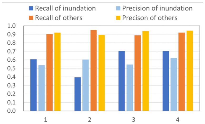
| (a) Multi-Temporal Comparison | |||||
|---|---|---|---|---|---|
| Ground Truth [km2] | |||||
| Inundation | Others | Total | Precision | ||
| The extracted results [km2] | Inundation | 5.76 | 4.98 | 10.74 | 53.6% |
| Others | 3.73 | 44.83 | 48.56 | 92.1% | |
| Total | 9.49 | 49.81 | 59.30 | ||
| Recall | 60.7% | 90.0% | 85.3% | ||
| (b) Mono-Temporal Determination | |||||
| Ground Truth [km2] | |||||
| Inundation | Others | Total | Precision | ||
| The extracted results [km2] | Inundation | 3.75 | 2.47 | 6.22 | 60.3% |
| Others | 5.74 | 47.34 | 53.08 | 89.2% | |
| Total | 9.49 | 49.81 | 59.30 | ||
| Recall | 39.5% | 95.0% | 86.2% | ||
| Ground Truth [km2] | |||||
|---|---|---|---|---|---|
| Inundation | Others | Total | Precision | ||
| The extracted results [km2] | Inundation | 6.68 | 5.55 | 12.23 | 54.6% |
| Others | 2.81 | 44.26 | 47.07 | 94.0% | |
| Total | 9.49 | 49.81 | 59.30 | ||
| Recall | 70.4% | 88.9% | 85.9% | ||
| (a) Verification Using the Inundation Boundary of the GSI. | |||||
|---|---|---|---|---|---|
| Ground Truth [km2] | |||||
| Inundation | Others | Total | Precision | ||
| The extracted results [km2] | Inundation | 20.28 | 34.44 | 54.72 | 37.1% |
| Others | 7.71 | 180.98 | 188.69 | 95.9% | |
| Total | 27.99 | 215.42 | 243.41 | ||
| Recall | 72.5% | 84.0% | 82.7% | ||
| (b) Verification Using the Inundation Polygon of the MLIT. | |||||
| Ground Truth [km2] | |||||
| Inundation | Others | Total | Precision | ||
| The extracted results [km2] | Inundation | 29.79 | 31.67 | 61.46 | 48.5% |
| Others | 10.42 | 211.58 | 222.00 | 95.3% | |
| Total | 40.21 | 243.25 | 283.46 | ||
| Recall | 74.1% | 87.0% | 85.2% | ||
Publisher’s Note: MDPI stays neutral with regard to jurisdictional claims in published maps and institutional affiliations. |
© 2021 by the authors. Licensee MDPI, Basel, Switzerland. This article is an open access article distributed under the terms and conditions of the Creative Commons Attribution (CC BY) license (http://creativecommons.org/licenses/by/4.0/).
Share and Cite
Liu, W.; Fujii, K.; Maruyama, Y.; Yamazaki, F. Inundation Assessment of the 2019 Typhoon Hagibis in Japan Using Multi-Temporal Sentinel-1 Intensity Images. Remote Sens. 2021, 13, 639. https://doi.org/10.3390/rs13040639
Liu W, Fujii K, Maruyama Y, Yamazaki F. Inundation Assessment of the 2019 Typhoon Hagibis in Japan Using Multi-Temporal Sentinel-1 Intensity Images. Remote Sensing. 2021; 13(4):639. https://doi.org/10.3390/rs13040639
Chicago/Turabian StyleLiu, Wen, Kiho Fujii, Yoshihisa Maruyama, and Fumio Yamazaki. 2021. "Inundation Assessment of the 2019 Typhoon Hagibis in Japan Using Multi-Temporal Sentinel-1 Intensity Images" Remote Sensing 13, no. 4: 639. https://doi.org/10.3390/rs13040639