
Multi-Temporal Small Baseline Interferometric SAR Algorithms: Error Budget and Theoretical Performance


Institute for Electromagnetic Sensing of the Environment (IREA), Italian National Research Council, 328, Diocleziano, 80124 Napoli, Italy
Remote Sens. 2021, 13(4), 557; https://doi.org/10.3390/rs13040557
Submission received: 23 December 2020
/
Revised: 26 January 2021
/
Accepted: 28 January 2021
/
Published: 4 February 2021
(This article belongs to the Collection Feature Papers for Section Environmental Remote Sensing)
Abstract
:Multi-temporal interferometric synthetic aperture radar (MT-InSAR) techniques are well recognized as useful tools for detecting and monitoring Earth’s surface temporal changes. In this work, the fundamentals of error noise propagation and perturbation theories are applied to derive the ground displacement products’ theoretical error bounds of the small baseline (SB) differential interferometric synthetic aperture radar algorithms. A general formulation of the least-squares (LS) optimization problem, representing the SB methods implementation’s core, was adopted in this research study. A particular emphasis was placed on the effects of time-uncorrelated phase unwrapping mistakes and time-inconsistent phase disturbances in sets of SB interferograms, leading to artefacts in the attainable InSAR products. Moreover, this study created the theoretical basis for further developments aimed at quantifying the error budget of the time-uncorrelated phase unwrapping mistakes and studying time-inconsistent phase artefacts for the generation of InSAR data products. Some experiments, performed by considering a sequence of synthetic aperture radar (SAR) images collected by the ASAR sensor onboard the ENVISAT satellite, supported the developed theoretical framework.
1. Introduction
Differential synthetic aperture radar interferometry (DInSAR) [1,2,3,4] is a consolidated methodology for the detection and constant monitoring of Earth’s surface ground displacements and the surveillance of infrastructures damage [5,6,7,8,9,10,11,12,13,14,15]. In recent years, the growing availability of RADAR images collected by constellations of synthetic aperture RADAR (SAR) satellites, which operate at different electromagnetic frequency bands and complementary acquisition modes, led to the flourish of a variegated series of DInSAR applications and novel technological developments. In particular, over the last twenty years, the DInSAR technology gradually evolved towards new advanced multi-temporal interferometric SAR (MT-InSAR) techniques [16,17,18,19,20,21,22,23,24,25,26,27,28,29,30,31,32,33,34,35], for the generation of ground displacement time-series. In this context, the two main classes of the Persistent Scatterers (PS) [21,36] and the Small Baseline (SB) [16,25,26,27,37,38,39] methods emerged, and were principally used for the detection of the displacements affecting point-wise persistent scatterers (PS) and distributed scatterers (DS) on the terrain, respectively. On the one hand, the PS methods analyzed the displacement of SAR scenes’ radar pixels, at the single-look resolution scale, characterized by a dominant scatterer that maintained its phase stability over the entire SAR data time-series. On the other hand, the SB methodologies allowed the analysis of the ground displacement of DSs on the ground, which might be affected by spatial and temporal decorrelation [40,41]. For this purpose, the SB methods select multiple-master InSAR data pairs characterized by short temporal and spatial baselines, thus preserving their coherence and facilitating the extraction of useful information on the phase history of distributed targets on the scene. Furthermore, the SB interferograms are usually multi-looked (complex averaged) [3] to mitigate the decorrelation phase noise effects.
More recently, with the scope of maximizing the total number of correctly investigated DS pixels, novel MT-InSAR techniques, based on the processing of long sequences of optimized multi-looked DInSAR interferograms, also emerged, such as SqueeSAR [22], CAESAR [23], and other alternative methods [29,32,42]. Some cross-comparison analyses of the different, developed MT-InSAR techniques [43,44,45,46,47] were also carried out to quantitatively assess their mutual performances. Moreover, in the last seven years, the InSAR community was primarily focused on adapting the available MT-InSAR codes to process large sequences of SAR data collected by the new constellations of SAR satellites. In particular, a significant role was played by the Sentinel-1A/B (S-1) twin satellites of the European Union Copernicus initiative [48]. The free and open access policy of the S-1 data and the weekly repetition frequency of the observations contributed to InSAR technology’s evolution to afford the challenges of the present-day, big-data era. New developments are required to adapt the existing processing codes to handle Interferometric Wide (IW) Swath S-1 SAR data. These were collected through the Terrain Observation with Progressive Scans (TOPS) mode [49], which is the principal acquisition mode of S-1 over lands. In this context, several studies were performed to demonstrate the S-l SAR data’s potential for global mapping and the effective processing of large sequences of TOPS SAR data [50,51,52]. Despite the high capability of the MT-InSAR techniques to measure displacement phenomena, there are still open questions to be theoretically addressed. For instance, it is worth mentioning the recent developments based on the use of InSAR data, at different polarizations, for the extraction of additional information on some underlying geophysical phenomena, such as for the retrieval of soil-moisture parameters of the imaged scenes from InSAR data [53,54,55,56].
This research study aimed to investigate, from a theoretical perspective, the error bounds of the ground deformation InSAR products, e.g., mean displacement maps and relevant ground deformation time-series, obtained using the small baseline (SB) methods. The different contributions of the unwrapped phases of the identified set of SB InSAR data pairs were thoroughly investigated, focusing on the decorrelation of noise sources. The role of the time-correlated and time-uncorrelated disturbance phase terms in the set of SB interferograms was also discussed, to study how these terms could affect the quality of the reconstructed ground deformation time-series via the multi-temporal SB InSAR techniques. Indeed, the time inconsistencies in the set of unwrapped SB interferograms might lead to erroneous InSAR products. Nevertheless, in the case of the Small Baseline Subset (SBAS) [25] algorithm, the temporal coherence is typically used as a quality index of the retrieved ground deformation time-series [57]. In particular, the temporal coherence values could be used to eventually identify a group of reliable and well-processed SAR pixels after the SBAS inversion. Invoking the principles of error noise propagation [58] and perturbation theory [59,60,61,62], the ground deformation InSAR products’ relative error was eventually retrieved. It was mathematically and statistically demonstrated that this error depends on the properties of the SB unwrapped phases and the design matrices of the identified networks of SB interferograms. This work also put the basis for future investigations assessing the potential and efficiency of SB methods in recovering additional geophysical information on the imaged scene’s state. The algebraical and statistical properties of the inversion procedures adopted by the SB algorithms to recover the wanted ground deformation products were addressed to this aim.
This paper is organized as follows. Section 3, Section 4 and Section 5 quantify the error budget of SB methods for the ground displacement of InSAR products. Section 6 presents the results of some experiments performed to support the recovered theoretical outcomes. Finally, a short discussion on the study outcomes and future perspectives are presented in Section 7 and Section 8.
2. The SB InSAR Framework
In this section, the basic rationale of SB methods and the SB multi-looked phase characterizations are provided. First, let us consider a set of SAR images collected at times , which are adequately re-sampled on the same reference image grid, and let be the complex data vector:
where is the complex reflectivity of the i-th SLC image computed at the generic radar pixel , and is the transposition operator. Starting from the available SAR images, and for every radar pixel , the sample covariance data matrix [63] could be calculated as:
where is the expectation operator, is the group of samples in the neighborhood of the given radar pixel used for the computation of the expectation value in (2), and represents the cardinality of ; note also that is the complex Hermitian operation. Some recent advanced methods [22,64,65,66] for the proper, spatially-adaptive identification of a set of statistically homogenous pixels (SHPs), could also be employed for the efficient computation of the sample covariance data matrix, see Equation (2).
Remarkably, the off-diagonal elements of the upper (lower) triangular matrix derived from the covariance matrix corresponded to the entire set of possible complex multi-looked interferograms that could be generated from the set of available SAR images. Specifically, the -th element of the covariance matrix was given by:
where is the (wrapped) multi-looked interferogram related to the SAR data pair and is the coherence [41,67] of the relevant interferometric SAR data pair. Moreover, let and be the perpendicular and temporal baselines of the -th interferometric SAR data pairs.
Among the vast amount of interferometric SAR techniques developed in almost the last thirty years to study the Earth’s surface displacements, the class of small baseline (SB) methods, see for instance [25,27,31,33,37,38], is widely used. The SB methods were principally developed to investigate the ground displacement signals of distributed targets (DS’s), which correspond to spatially-distributed objects on the ground with no dominant point-wise scatterers that are affected by the spatial and temporal decorrelation phenomena [40].
To partially circumvent the phase decorrelation problems, efficiently, the SB methods select only the differential SAR data pairs with short temporal and geometric baselines. As an example, Figure 1a shows a distribution of SB interferograms in the temporal/perpendicular baseline plane.
Let and be the data vector of the wrapped and unwrapped SB multi-looked interferograms, computed at the generic pixel . Note also that the subsequent SB interferograms’ inversion procedures are applied to every SAR pixel, independently. For this reason, the dependence on the coordinates of the given radar pixel P of the considered data vectors is not explicitly mentioned in this paper, from here on.
The different SB methods proposed in the literature have individual peculiarities; however, a unified representation must analyze their performances. Specifically, in this research paper, the general representation adopted in [44] is recognized as valuable and extensively adopted. The different implementations of the SB methods are unified considering that a linear transformation that relates the vector of the unwrapped SB interferograms, namely , with a model of unknown parameters of the ground deformation, is implemented. The adopted unified representation of the SB linear transformation is, hence, given by:
where is the design matrix of the linear transformation and is the vector of the model parameters values, with being the number of independent parameters that describe the adopted model. For instance, if we consider the pioneered small baseline subset (SBAS) algorithm [25], the model parameters are the velocities between consecutive time acquisitions, specifically , and the design matrix has the following expression [25]:
where and are the indices of the master and slave images of the i-th SB multi-looked interferogram, respectively, where it is assumed that . Again, for the SBAS case, the application of constraints on the maximum allowed temporal and spatial baselines of the interferograms can generally lead to the available SAR scenes clustered in the data subsets, separated by large baselines. In this case, the system of linear Equation (4) was solved in the least-squares (LS) sense, by decomposing the design matrix with the singular value decomposition (SVD) method [68,69]. As anticipated earlier in [44], a unified schema for the processing chain of four selected different implementations of SB methods were introduced, and the performances of the four methods were quantitatively compared. In particular, they mentioned the SB implementations developed in the StaMPS/MTI toolbox, and three independent implementations provided by the Giant toolbox.
In this research study, the author investigated the linear transformation’s algebraic properties of the system of linear Equation (4), intending to recover the theoretical upper bounds of the relative errors of the InSAR products’ measurements obtained using the SB methods. The dependence of those bounds on the selected threshold on the maximum allowed perpendicular baseline of the SB interferograms was also explored. Finally, for the SBAS method, the accuracy of the measurements as a function of the SB interferograms’ coherence and the temporal coherence of the generated InSAR products [57] was derived.
Let us start by introducing the statistical properties of the sequence of the unwrapped SB phase values . The i-th component of the vector of unwrapped phases could be expressed as [67,70]:
where:
is the proper (wanted) phase component related to the ground displacement that occurred between the two passes of the radar sensor over the illuminated scene, related to the i-th interferometric SAR data pair. In particular, if the ground deformation is assumed to be linear, with a mean displacement rate , this term could be approximated to, where is the operational radar wavelength and is the temporal span of the i-th SB InSAR data pair.
is the phase artefact related to the differential atmospheric phase screen (APS) between the two SAR images forming the i-th interferogram. Several studies already addressed the problem of studying and characterizing this phase contribution (see, for instance, [39,71,72]), both for satellite and ground-based radar systems, considering the atmosphere’s physical properties. These phase contributions are due to the inhomogeneities of the medium within the used electromagnetic waves propagation. Note that the spurious APS signals in a sequence of SAR data are almost spatially correlated and temporally uncorrelated, and the tropospheric contribution depends on the topography of the scene [70,72].
is the spurious contribution in an interferogram due to a non-perfect removal of the topographic phase term, during the differential interferogram formation [25,73]. It is related to the errors of the used digital elevation model (DEM) of the scene as: , where is the perpendicular baseline of the i-th interferogram, is the sensor-to-target range distance and is the local incidence angle of the electromagnetic waves on the terrain.
is the decorrelation phase, which could be categorized as due to geometrical, temporal, and volumetric effects and the radar instrument noise; see the works of [40,41,67] for a comprehensive review of the decorrelation causes and the methods developed to analyze and filter out these spurious phase terms in the generated (multi-looked) interferograms. Note that the scatterers’ phase noise correlates with interferograms having common SAR acquisitions. Accordingly, this phase noise contribution takes into account the temporally correlated noise, exclusively. It means that, ideally, for the phase noise term attained, a single redundant network of SB interferograms (see Figure 1) contains the same information as any other connected graph of the interferogram. Accordingly, this kind of phase noise contributions is representative of a temporally-conservative field.
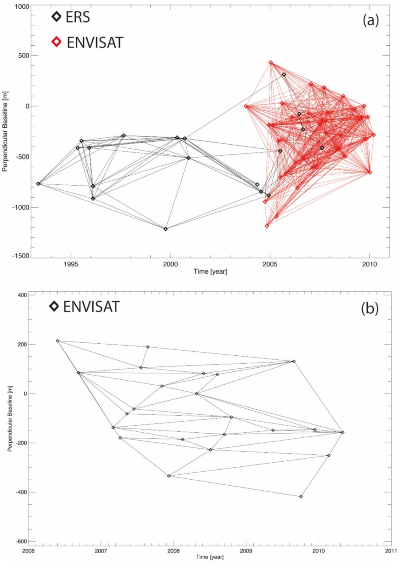
, on the other hand, is the contribution of the phase noise that is time-uncorrelated. Hence, these phase components are temporally inconsistent. It means that considering a triplet of SB interferograms generated from three SAR images (namely A, B, C), and forming a closed loop (namely AB, BC, CA), the sum of the relevant uncorrelated phase noise contributions differs from zero, namely [22,24,32,70], where the symbol is the wrapping operator (see Figure 2). This phase term is the composite effect of small random alterations that determine the temporal-inconsistency of statistical operations, such as those involved in the generation of multi-looked SB interferograms or due to systematic errors in the operations of co-registration and noise filtering of every single data pair, when these operations are independently applied to every single interferogram. Unlike these statistical inconsistencies, this phase noise contribution also takes into account a lack of consistency related to underlying physical reasons connected to the electromagnetic waves’ different scattering mechanisms with the imaged objects. Some recent works [53,74,75] investigated this problem from the statistical and physical point of view, shedding light on the potential application of these inconsistencies to retrieve some parameters of interest of the underlying physical phenomena.
Finally, the term accounts for the errors, due to the incorrect phase unwrapping operations, where is an integer representing the number of phase cycles that were incorrectly estimated during the phase unwrapping operations. It is worth emphasizing that phase unwrapping mistakes could be decomposed as the sum of two terms: . The former contribution, namely , considers the phase unwrapping mistakes that are temporally consistent. It means that considering the three A, B, C images pictorially shown in Figure 2, . On the contrary, the second component considers the temporally uncorrelated phase unwrapping mistakes, for which the following relation holds. It is also worth mentioning that some existing 3-D or hybrid phase unwrapping operations (e.g., [57]) can handle/manage/correct these uncorrelated phase unwrapping mistakes.
Of great concern for this investigation are the effects of the uncorrelated phase unwrapping mistakes and the uncorrelated noise phase terms on the linear system’s solution of Equation (4). Indeed, if the adopted model in Equation (4) is time-consistent, the time uncorrelated components are those responsible for the residuals of the relevant least-squares problem. On the contrary, the remaining time-correlated phase contributions ,, , and , although representative of distortions in the final solution, belong to the co-domain of the linear transformation (4) and, thus, they do not produce any phase residual after the LS optimization. To better clarify this relevant issue, let be the actual (wanted) signal, and , , , .
It is known that the solution of the LS problem in Equation (4) can generally be obtained as:
where is the (left) pseudo inverse of the design matrix obtained by applying SVD [69]:
with
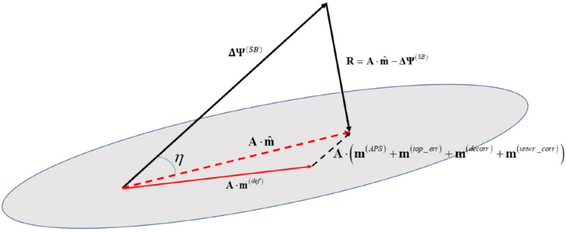
where is an orthonormal matrix, is an orthonormal matrix, and , where the elements on the diagonal of represent the singular values of the matrix and . The obtained LS solution guarantees that the vector of residues has a minimal norm, i.e., . More specifically, if the matrix has full rank, i.e., when the interferometric SAR data pairs are selected to form one single data subset, there exists one single data vector that minimizes the norm of the residual vector. That residual vector must necessarily be orthogonal to the space spanned by the linear transformation (see Figure 3).
Conversely, when the matrix has a rank-deficiency, there are infinite LS solutions with a minimal norm, and the application of SVD allows one identifying that LS solution with minimal two-norm residues and minimal norm, i.e., .
A few remarks concerning the temporal coherence factor [57] usually adopted by the SBAS algorithm are now discussed. As said, for the SBAS case and similar SB methods, the time-uncorrelated phase terms and the time-uncorrelated phase unwrapping errors lead to temporal inconsistencies in the final solution. For the SBAS algorithm [25], the temporal coherence factor was initially introduced in [57] to expressively quantify the effects of such temporal inconsistencies; hence, the temporal coherence factor represents a quality index of the ground displacement time-series reconstruction. Over the years, the temporal coherence was extensively used in several SBAS investigations, see for instance [76,77,78,79], to identify the reliable pixels after SBAS inversion. The temporal coherence factor was mathematically defined as:
where is the vector of the residues of the LS solution of the system of Linear Equation (4). Accordingly, the significant uncorrelated phase terms and phase unwrapping mistakes translated to low values of temporal coherence. Thus, those pixels with values of the temporal coherence below a fixed threshold (e.g., 0.7) were discarded from the consequent analyses.
For subsequent analyses, it is worth remarking that, given a real-valued vector of random samples, the two-norm of the vector [58] is given by:
3. Relative Error Bounds of Ground Deformation Measurements via the SB Methods
Let us now compute the relative error bounds of the InSAR product measurements via the SB methods. Invoking the principles of perturbation theory [60,61,62], it is known that the upper bound of the relative error for the (unknown) model parameters in the system of Equation (4), is generally given by:
where is the vector of the (unknown) true model parameters, is the condition number of the design matrix , is the non-zero smallest singular value of the matrix , is the relative error of the (input) vector of the SB unwrapped phases, and is the vector of the residues of the LS solution of Equation (4). Moreover, is the angle between the vector and the vector and measures whether the residual vector is large (i.e., near ) or small (near zero). The application of straightforward geometrical relationships allows the further manipulation of Equation (12) to obtain the following bound (see Figure 3):
From Equations (6) and (11), the relative error of the input data (i.e., the vector of the unwrapped phase data) in Equation (13) could be expressed as:
It is worth noting that the knowledge of the unwrapped phase vectors’ total covariance matrix would allow the comprehensive characterization of the output data vector statistical properties. Indeed [68]:
where the elements on the diagonal of get an estimate of the variance of every considered model parameter. Considering the different components of the unwrapped phases given by Equation (6), the total covariance matrix of the unwrapped phases could be suitably derived as:
where , ,,, are the covariance matrices for the atmospheric phase screen, the residual topography, the decorrelation noise, the time-uncorrelated phase signals, and the phase unwrapping mistakes, respectively. Equation (16) assumes the validity of the hypothesis of the statistical independence of the different components of the unwrapped phase vector ; this assumption is reasonable for the first three terms in Equation (16), which represent the unrelated physical processes, whereas the phase unwrapping mistakes could however be reasonably correlated to the decorrelation noise and the time-inconsistent phase signals in Equation (6). Remarkably, some noise models [70,80] were developed to compute and characterize the covariance matrix components of the time uncorrelated phase artefacts [53]. However, further efforts are still required to estimate the covariance matrix of the phase unwrapping mistakes from the data. This investigation makes it evident, from the mathematical and statistical point of view, that the residual phase vector depends on the time uncorrelated phase components of the unwrapped phases, i.e., and , and, hence, the temporal coherence, see Equation (10), could be effectively used as a proxy to derive, at least, the covariance matrix of the time uncorrelated phase components. Nonetheless, even though the total covariance matrix is of difficult estimation, an upper bound of the relative error of the model parameters could still be retrieved by merely making a profit from the algebraical properties of the system (4) and using Equations (13) and (14).
4. How Do the Relative Error Bounds Depend on the Perpendicular Baseline Threshold of the SB Interferograms?
Let us evaluate how the input data vector’s relative errors critically depend on the applied threshold on the selected SB interferograms’ maximum perpendicular baselines. To this aim, let us first consider the idealized case that (i) the APS and topographic phase components are not present, (ii) no phase unwrapping errors were committed during the phase unwrapping operations, and (iii) the uncorrelated phase terms were not relevant. Moreover, to study the dependence of the errors on the perpendicular baseline, exclusively, let us assume that the geometric decorrelation noise was the dominant contribution of the time-correlated phase component . In this idealized case, Equation (14) is particularized as:
Equation (17) could be further manipulated considering the Cramer Rao bound on the phase decorrelation variance [41], which is given by:
where is the coherence of the k-th interferogram that could be expressed as a function of the interferogram perpendicular baseline as:
where is the critical baseline [3]. Taking into account Equations (18) and (19), Equation (17) could then be re-expressed as follows:
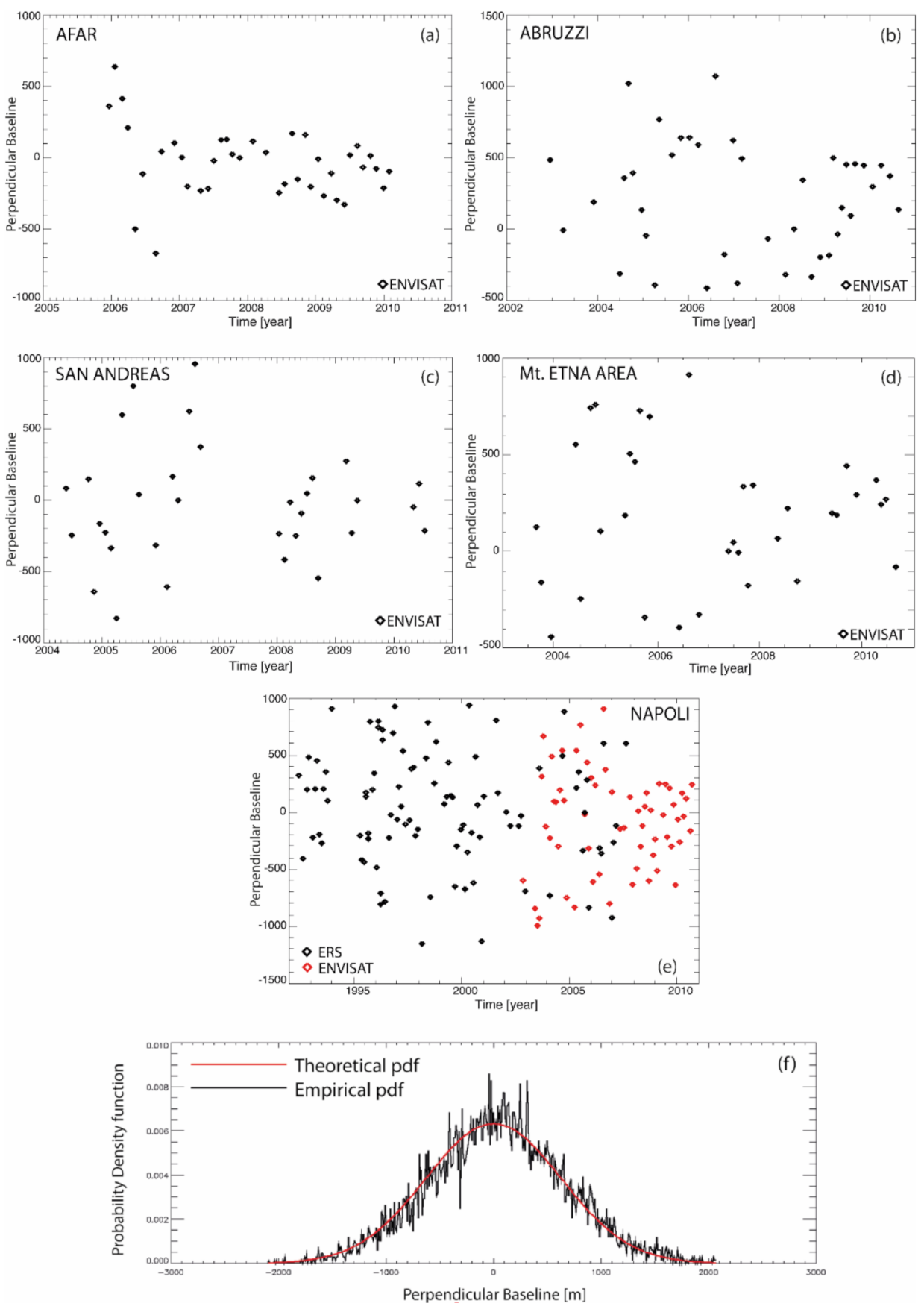
Given a distribution of SAR images, one could infer the statistical distribution of the absolute value of the interferograms’ perpendicular baselines. A previous work [81] already addressed this problem, by using the Kolmogorov-Smirnov test [58] and showing that, with a certain degree of confidence, the absolute value of the perpendicular baselines might be inferred to as distributed with an exponential probability density function (pdf). Additional investigations, carried out considering larger sets of SAR data acquired by the ERS and ENVISAT sensors revealed that, by invoking the central theorem limit [58], the baseline could be inferred to be distributed with a zero-mean normal density function. Figure 4f shows the perpendicular baselines’ theoretical and empirical pdfs inferred from a set of 237 SAR images collected by the first-generation ERS and ENVISAT European Space Agency (ESA) sensors. The perpendicular baseline empirical pdf was directly derived from the data (black line), whereas the relevant theoretical pdf (red line) was inferred to be distributed with a zero-mean normal distribution:
This statement’s validity was inferred from the available data by applying the Kolmogorov-Smirnov test [82] on the normality, where , the standard deviation of the distribution, was equal to about 600 m in the experiments shown in Figure 4. Following Equation (19), there was complete decorrelation when the perpendicular baseline value exceeded the critical baseline value .
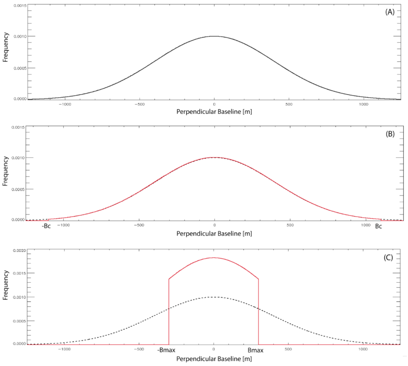
For the practical implementation of an SB method, a threshold on the maximum perpendicular baseline of the interferometric SAR data pairs is imposed. This circumstance leads to the conclusion that the successfully used InSAR data pairs had their perpendicular baselines distributed with a truncated normal distribution (see Figure 5), as:
After straightforward mathematical manipulations, it could be shown, for medium-to-high coherence values, that a good approximation for the expected value of the term was given by:
where:
Note that Equation (23) was obtained by a Taylor series expansion of the function , see Equation (18), and is the expansion’s order. Figure 6 shows the plot of versus the selected maximum perpendicular baseline of the SB interferogram, numerically obtained by considering a series expansion of order five, and different values of the perpendicular baselines’ standard deviation.
By substituting Equation (23) in Equation (20), the relative error of the input data is retrieved in this idealized case, as follows:
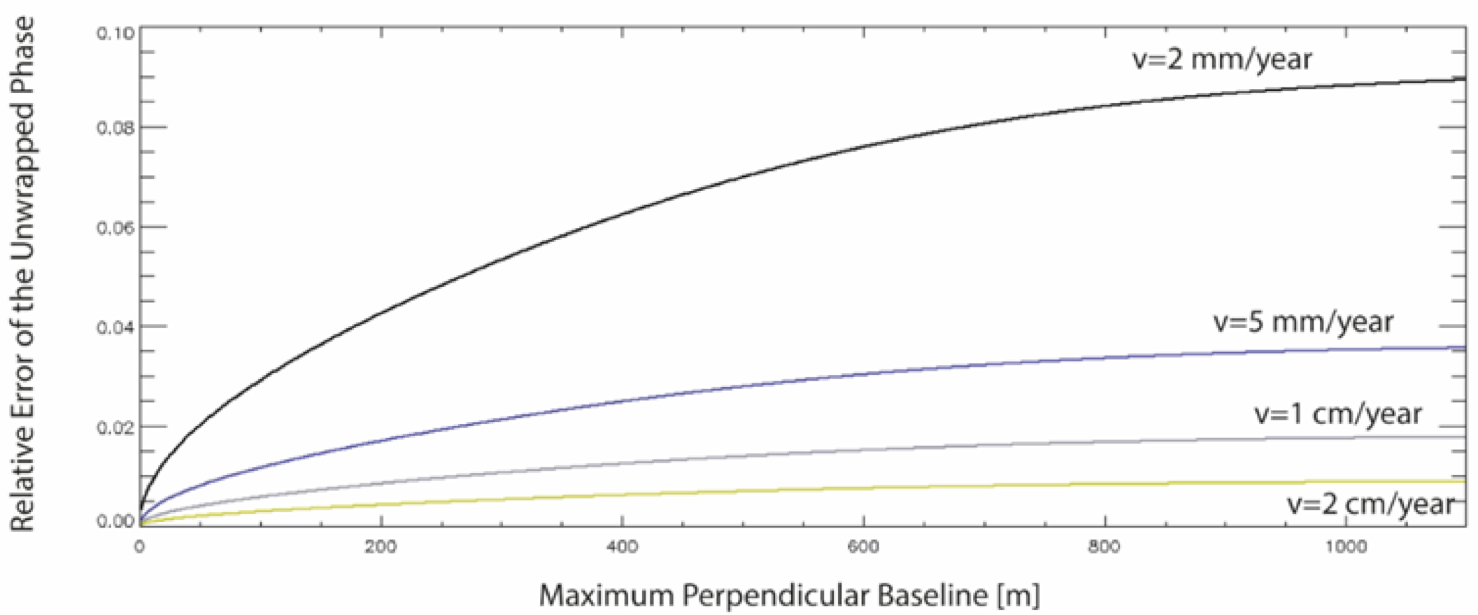
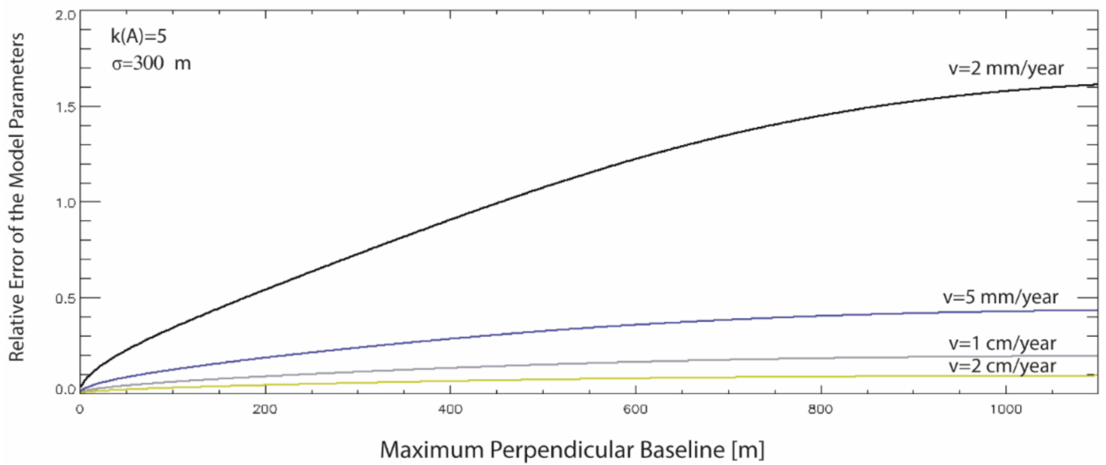
where the following approximation was also considered. From Equation (27), it could be seen that the relative error of the input data depended on the operating wavelength and the mean deformation velocity , as well as on the selected maximum perpendicular baseline value . Figure 7 shows the plot of the relative error versus the selected maximum perpendicular baseline for the different values of the mean deformation velocity of the given point on the ground, considering a SAR platform operating at the C-band, with a wavelength of about 5.6 cm of the transmitted signals, a multi-look factor , an InSAR temporal average root mean squared value equal to , and a value of the standard deviation of the perpendicular baseline equal to 300 m. The considered parameters were relevant to the first-generation C-band SAR sensors, but similar calculations could be adapted to the new generation of SAR sensors.
In this idealized case, it is essential to note that, as expected, the information related to small ground deformation rates (smaller than 1 mm/year) could be recovered in the generated interferograms but with higher relative errors. Short perpendicular baseline values are preferable, even though very short baselines are not realistic in a conventional case. Additionally, very short baselines, except for limited cases, could not be recommended because design matrices with higher condition numbers were more likely to characterize the SB interferograms’ relevant networks, which harm the estimated model parameter vector’s correctness .
As anticipated, the calculations provided here only took into account the geometrical decorrelation effects. A more comprehensive estimate of the “input” errors of the system of Linear Equation (4) that also considered the effects of other decorrelation noise sources and the phase unwrapping mistakes is given below.
In more general case, the error bound of the (wanted) model parameters in Equation (4) is given, see Equation (14), by:
where
Some further remarks on the terms on the right-hand side of Equation (29) are now addressed. As earlier said, the term only takes into account the geometrical phase decorrelation effects in the generated interferograms. However, the total decorrelation is quantified by the estimated coherence values of the (multi-looked) SAR interferograms, namely , which could be factorized as [67]:
where takes account of the spatial decorrelation, is the temporal decorrelation, and is the thermal decorrelation component. The Cramer Rao bound for the phase variance of the temporal decorrelation noise is then given by:
Similar to what was formerly done for the estimation of the component relevant to the geometrical decorrelation effects, it could be straightforwardly demonstrated that:
where:
For the attained norm of the residual topographical mistakes , the application of the InSAR basic principles [73] allowed demonstrating that:
Concerning the norm of the APS contribution, its calculation required further considerations relying on the distinction between the tropospheric and ionospheric terms; a model is provided in [70] (and references therein). For the tropospheric components, one could say that is linearly dependent on the height of the scene, say , and the slant-range distance between the observed point and a reference pixel in the area (for instance, the pixel to which the ground deformation measurements are calibrated). Accordingly, , where and are appropriate constants to be computed.
Further extensive studies are still required to compute the covariance matrix of the temporally-correlated phase unwrapping problems, which do not lead to temporal inconsistencies in the system of Linear Equation (4) and, hence, are difficult to be extracted and studied. Several studies on the phase unwrapping topic, including both conventional, two-dimensional, and recently developed three-dimensional (space-time) approaches, are proposed in the literature, see for instance [57,83,84,85,86,87].
5. How Does the Temporal Coherence Get Valuable Information on the SBAS-InSar Products Error?
In this section, the problem of relating the LS residual data vector after the SB interferograms’ inversion with the relevant error source noise is addressed. As earlier anticipated in Section 2, in the SBAS case, such residuals are exclusively related to the time-uncorrelated phase terms . This means that the optimal LS solution of Equation (4) satisfies the following condition (see again Figure 3):
Accordingly:
From Equations (35) and (36), the phase residuals after the LS inversion (4) could be directly related to the time-uncorrelated phase terms of the unwrapped phases. More specifically:
At this stage, it is instructive to show that the temporal coherence, see Equation (10), computed after the SBAS inversion of the stack of unwrapped phases, gets a measure of the consistency between the original interferograms and those reconstructed from the obtained ground deformation time-series.
Considering the fundamentals of directional statistics [88], the temporal coherence could also be reformulated as:
where is the average residual phase, namely . Therefore, from Equation (38), the residuals’ norm could be expressed as a function of the temporal coherence values and the average phase residuals could be expressed as .
By summarizing, this research work leads to the conclusion that a suitable upper bound of the relative error of the SBAS (and the alternative SB methods) ground deformation measurements is given by:
where:
with
Equation (40) relies on the simplifying assumption that all unwrapped phase vectors’ contributions are independent. A few remarks on Equations (39)–(41) are now in order. Different contributions influence the relative error of the input data vector. It is worth noting that the temporal coherence value that appears in Equation (41) allows one to quantify the global effects of time-uncorrelated phase signals (i.e., phase unwrapping mistakes and time-uncorrelated wrapped phases) on the final solution and the network of SB interferograms. Moreover, the temporal coherence value also depends on the applied threshold on the maximum perpendicular baseline of the selected SB; however, that relationship is more challenging to extract. Further studies are still required to recover the closed-form mathematical relationships existing among these errors and the perpendicular baseline of the selected interferometric SAR data pairs.
Figure 8 shows the estimated model’s relative error as a function of the selected threshold on the SB interferograms’ maximum perpendicular baseline, in a simplified case.
This was obtained from Equation (40), without considering the contributions of the APS, the residual topography, and the time-correlated phase unwrapping mistakes, and assuming that the temporal coherence was equal to 1 (i.e., the idealized condition that no residuals were present after the LS inversion). Low values of the temporal coherence corresponded through Equation (40), to higher relative errors of the model parameters (4). Moreover, it is worth remarking that the variation of the condition number of the design matrix as the maximum perpendicular baseline decreases, was not included in the simulated results shown in the plot of Figure 8. Remarkably, SB networks with very short baselines constraints were less redundant than those with larger baselines. This implied a limit on the use of very short baselines, which is challenging to quantify from a theoretical point of view. In Section 6, some experiments were performed to show how the SB network’s condition number varied in a real scenario. Accordingly, a balance between opposite requirements must be adequately considered in selecting the most suitable threshold of the perpendicular baseline constraint. This investigation’s outcomes also deserve further analyses to include other mechanisms, such as suitable models accounting for the scenes’ temporal decorrelation, which were not considered. Of course, the complete characterization of the measurement errors requires the perfect knowledge of the total covariance matrix of the unwrapped phases, including the contributions of phase unwrapping errors, and this is a matter for other investigations.
Giving the implementation of the problem in Equation (4) provided within the SBAS algorithm, it is also instructive to finally derive the absolute error upper bound of the model parameters estimates. For the SBAS case, the model parameter vector contains the velocities between consecutive time acquisitions. Accordingly, if we consider a point on the ground subject to a perfectly linear displacement v, all vector velocity components were the same and were equal to the mean deformation velocity of the analyzed pixel, namely v. Therefore, considering the approximation provided in Equation (40), one could express the bound for the (average) absolute error of the model parameter, in the case that the terrain deformation was not zero, such as:
In the experimental section, the results of a series of tests are shown. Experiments were carried out to demonstrate how the SBAS (and potentially other alternative SB implementations) measurements’ quality, measured in terms of the temporal coherence, changed as the selected maximum perpendicular baseline of the SB InSAR data pairs became shorter.
6. Experimental Results
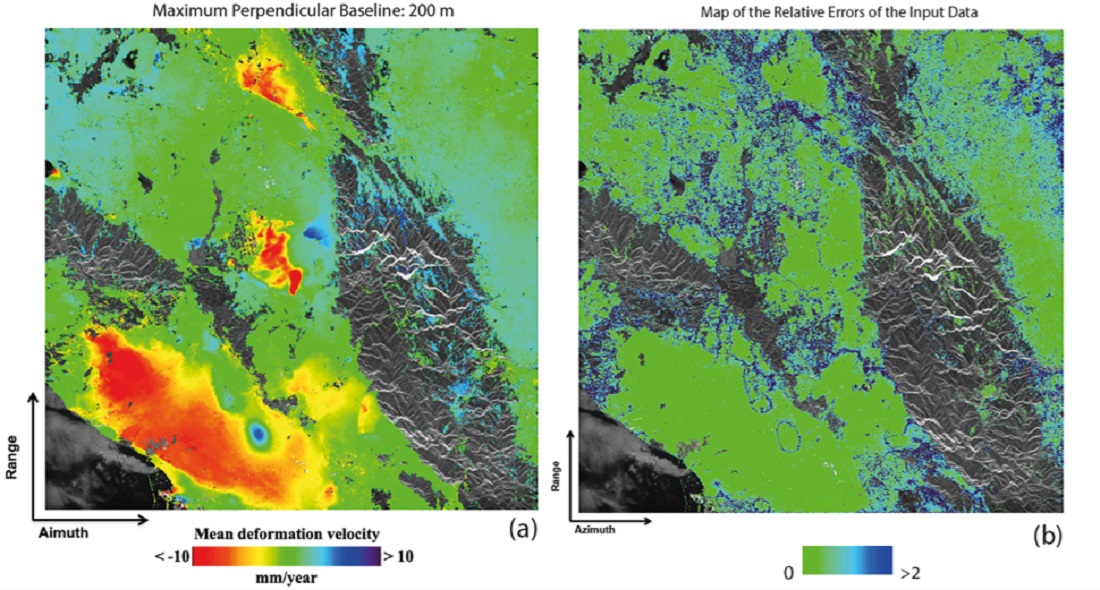
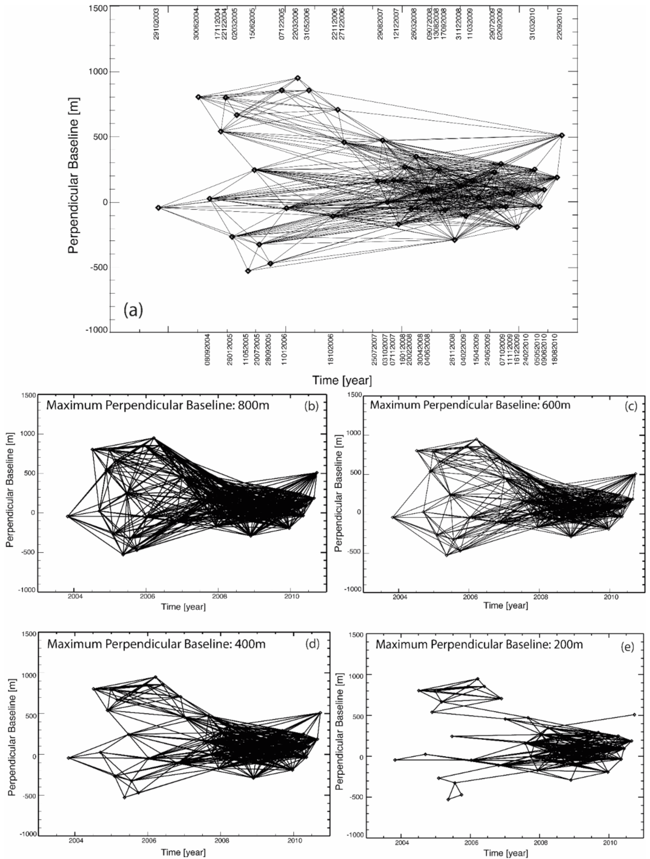
Some experiments were performed by processing a set of real SAR data to support the previous sections’ theoretical outcomes. In particular, this research study used a set of 48 ASAR images (ascending passes, Track 120, VV polarization) collected between 2003 and 2010 in the Southern California region. Figure 9 shows the distribution of the SAR scenes in the time/perpendicular baseline plane. Starting from the available SAR images, a group of 729 InSAR data pairs, characterized by a maximum temporal separation of 1000 days and a perpendicular baseline value smaller than the critical value (which was about 1100 m for a flat terrain in the case of the ENVISAT satellite) were selected and generated. The topographic phase components in the generated interferograms were reconstructed using precise satellite information, and a three-arc digital elevation model (DEM) of the investigated zone. To reduce the impact of phase noise artefacts in the interferograms, the generated interferograms were independently multi-looked (with forty azimuth looks and eight range looks, respectively) and filtered using the well-known Goldstein filter [89]. To show that the quality of the reconstructed ground deformation InSAR products enhanced, as the selected maximum allowed perpendicular baseline threshold of the SB interferograms decreased, some tests were done. The SBAS inversion procedure [25] was applied to the subsequently-reduced sets of SB interferograms, selected by progressively decreasing the maximum allowed perpendicular baseline of the interferograms.
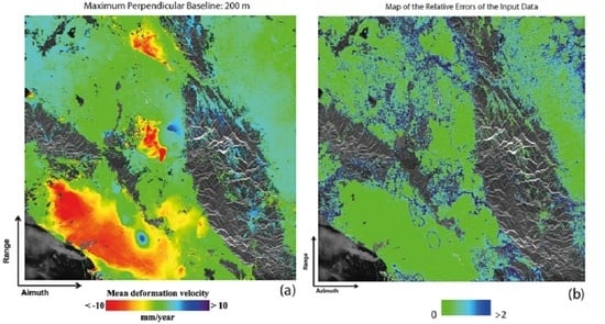
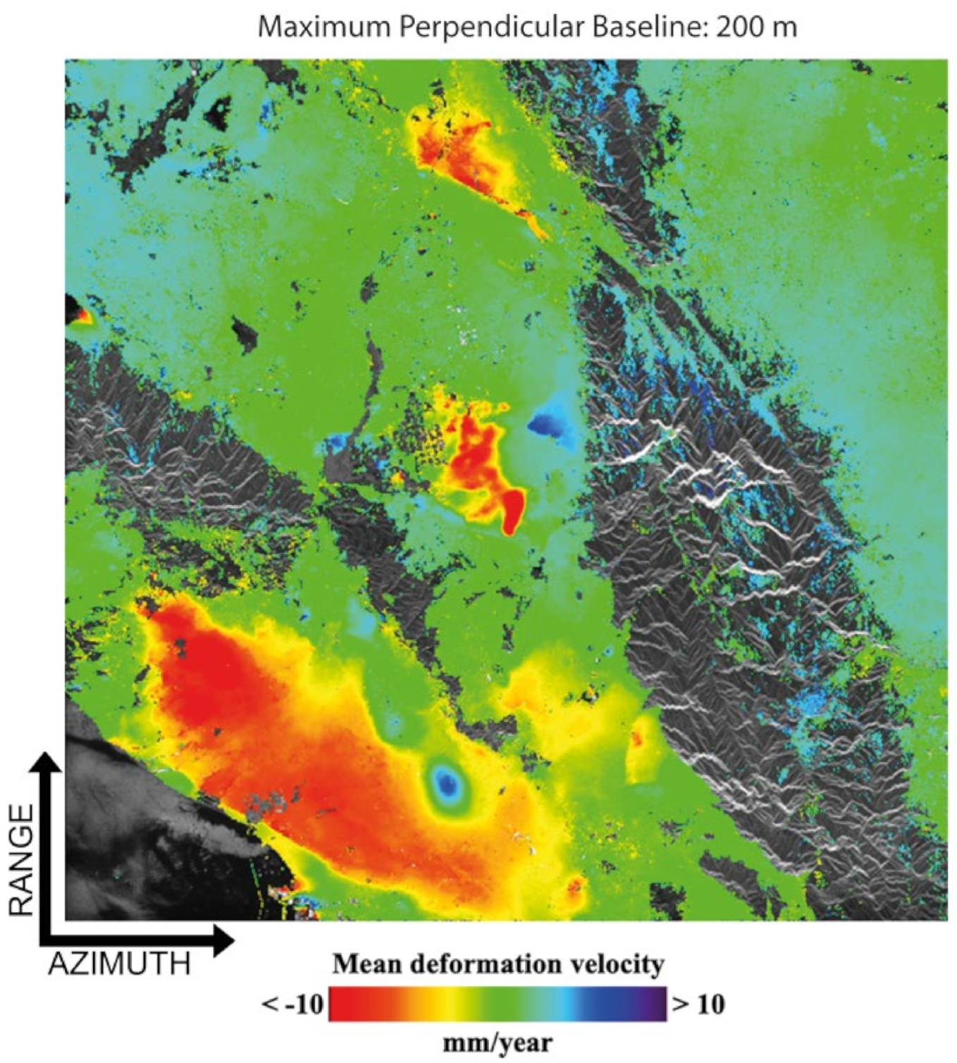
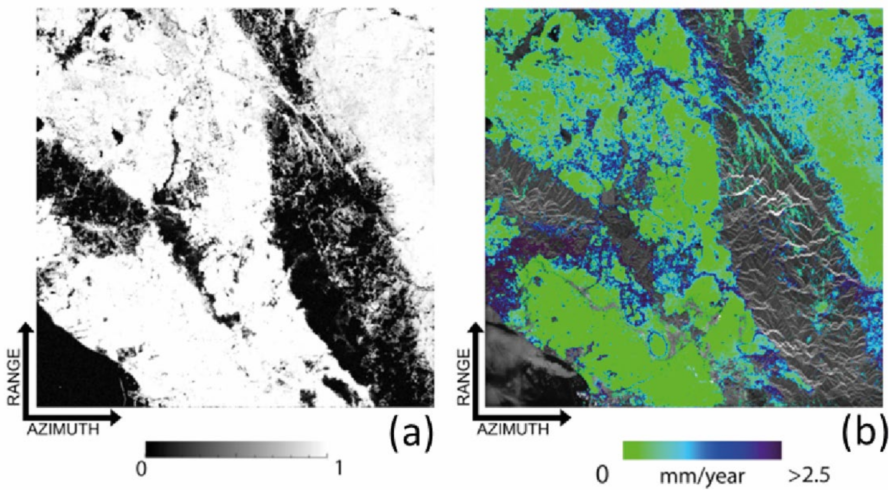
Figure 9 shows the selected InSAR data pairs’ distribution in the temporal/perpendicular baseline plane for the five tests performed by considering thresholds of 1100 m, 800 m, 600 m, 400 m, and 200 m on the maximum perpendicular baseline of the SB InSAR data pairs, respectively. The total group of 729 differential SAR interferograms, with a time separation shorter than 1000 days, were preliminarily, and independently, unwrapped using, for the sake of simplicity, the minimum cost flow phase unwrapping method proposed in [90]. For every set of SB interferograms, the SBAS inversion procedure was applied, and the relevant ground deformation time-series and the associated temporal coherence maps were obtained. As an example, Figure 10 shows the mean deformation displacement map of the area obtained by processing the group of interferograms shown in Figure 9e that corresponded to a threshold on the maximum perpendicular baseline of 200 m. The map shows the ground displacement information related to 228,318 well-processed radar pixels, exhibiting a temporal coherence value higher than 0.7, which was a suitable threshold.
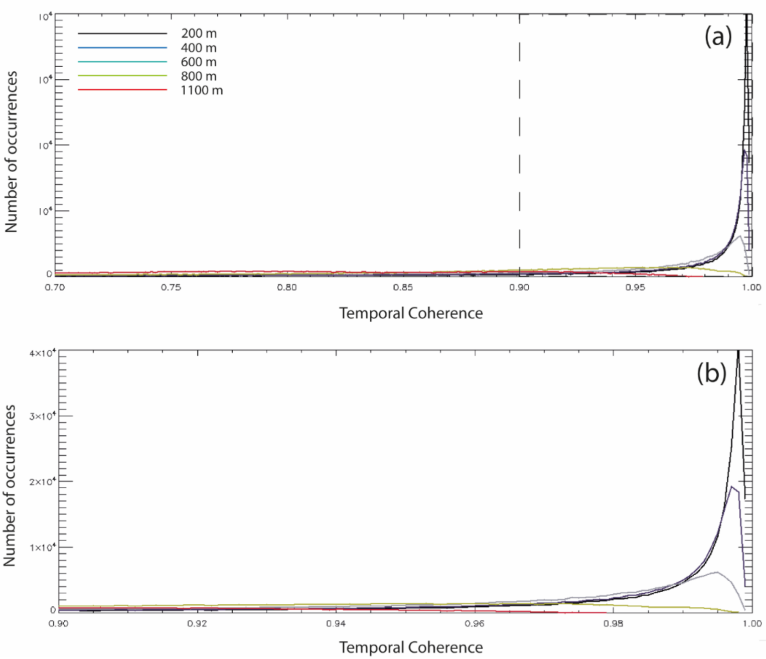
Figure 11 shows the comparison between the histograms of the temporal coherence value as a function of the applied maximum baseline constraints. The results of Figure 11 show how the use of different (higher) thresholds of the temporal coherence leads to identifying more reduced sets of well processed, reliable measurement points. Usually, a coherence threshold of 0.7 is used as a good compromise between the attainable density of the measurement points and the false alarm probability. Indeed, Equation (42) shows that higher temporal coherence values correspond to results with reduced errors. Specifically, the achieved results show how the (average) temporal coherence increased as the selected maximum perpendicular baseline decreased. However, it is remarkable that this threshold could not be decreased indefinitely, even though the number of detectable well-processed pixels increased considerably. Indeed, as the maximum allowed perpendicular baseline of the SB interferograms decreased, the number of SB interferograms reduced and, accordingly, the variance of the temporal coherence estimator tended to become significant, thus the measured temporal coherence results were biased. Indeed, it could be demonstrated that the variance of the temporal coherence estimator was approximately given by .
Moreover, as said in the previous section, very short baselines might reasonably lead to a design matrix with large condition numbers , affecting the obtained measurement quality. This statement agreed with that prescribed by Equation (42). Indeed, the second term on the right-hand side of Equation (42) (accounting for the temporal coherence ) is directly proportional to .
The map of the input data vector’s relative error , for the test-case with a 200 m-threshold on the maximum InSAR perpendicular baseline, is also shown in Figure 12. The relative error was estimated from the input data, using the following Equation:
where the variances of the interferograms were computed from the measured coherence values of the interferograms using the Cramer Rao bound limit for the phase variance, see Equation (18), and assuming the ground deformation was almost linear with a mean deformation velocity value v, which is shown in the map of Figure 11, obtained by fitting the recovered SBAS ground displacement time-series with a time linear model.
For the sake of simplicity, in Equation (36) and for the derivation of the input data relative errors, the effects of the time-correlated phase unwrapping errors, the APS, and the residual topography were neglected.
Figure 12 shows that the relative errors in the analyzed scene’s coherent regions were significantly reduced. Figure 12 only portrays the relative error of the well-processed SAR pixels with temporal coherence values larger than 0.7. In this case, = 1616 and ; accordingly, considering Equations (39)–(43), for SAR pixels with a temporal coherence of 0.7, the error bounds for the velocity deformation [rad/s] was about seven times larger than and was reduced to about 1.5 times the value of for coherence values larger than 0.85.
By using Equations (39)–(43), the error bound of the (average) absolute error of the measured ground mean displacement rate was retrieved for all well-processed SAR pixels selected with a temporal coherence threshold of 0.7. Figure 13a shows the map of the temporal coherence and Figure 13b shows the estimated map of the error for the velocity measurements obtained using the SBAS method. Over the whole set of 228,318 coherent and well-processed SAR pixels (with a temporal coherence larger than 0.7), an average error of 1.6 mm/year was obtained, which was in agreement with the results of experimental studies that showed that the average accuracy of SBAS measurements of the terrain displacement velocity was about 1 mm/year.
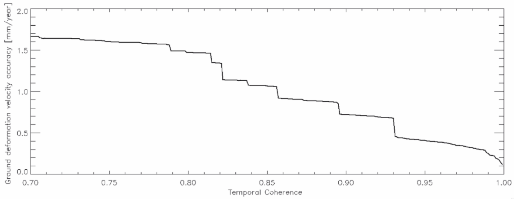
It is worth stressing that the values found in this research study represent the upper bounds of the InSAR products; hence it could be suitably affirmed that the SBAS accuracy (and of the SB methods alternative to SBAS) was on the order of 1 mm/year and in very coherent regions, also at sub-millimetric scale. To demonstrate this statement’s validity, Figure 14 shows the plot of the ground displacement velocity accuracy vs. the temporal coherence of the well-processed SAR pixels exceeding the threshold of 0.7. The plot makes it evident that accuracy improves as temporal coherence increases and for temporal coherence values of about 1 mm/year, which is what quantitative cross-comparison analyses demonstrate [76].
7. Discussion
This research study investigated the quality of InSAR ground deformation products obtained via multi-temporal interferometric small baseline algorithms. Fundamentals of error propagation theory and perturbation theory were exploited to retrieve some mathematical relationships relating the quality of the ground displacement model parameters to the operational wavelengths, satellite and scene image parameters, the relative error of the unwrapped phase vectors, and the characteristics of the used network of SB interferograms. It was shown that the SBAS algorithm’s performance and other alternative SB methods could be quantitatively evaluated by the measured value of the temporal coherence. Moreover, it was proven that networks of short baselines could guarantee improved performance, instead of using the whole set of potential InSAR interferograms with baseline values shorter than the critical ones. The research also demonstrated with real SAR data that the temporal coherence factor could be used as a proxy for the quantitative estimation of the error bounds of the time-correlated phase unwrapping and phase noise artefacts in the generated SBAS InSAR deformation products.
This research study’s primary outcomes could be extended to sets of the new generation of Sentinel-1 (S-1) SAR data and the forthcoming missions’ SAR data. The relative and absolute error bounds of the SB InSAR data products could generally be computed via Equations (39)–(43). Specifically, by processing the S-1 data [91], some peculiarities arose from the burst-mode TOPS acquisition of the IW S-1 SAR images that required intra-burst/inter-burst fine co-registration procedures [51]. Therefore, uncompensated time-uncorrelated misregistration mistakes in the sequence of the available S-1 SAR images, if not adequately compensated for [52], might introduce sensible, additional, time-uncorrelated phase artefacts in the set of unwrapped S-1 interferograms, see the term of Equation (6). Note also that S-1 is intrinsically an SB system because the S-1 orbital tube is narrow. This is beneficial for the achievable results, as also demonstrated by this research study, because a highly time-redundant network of SB interferograms is characterized by enhanced coherence and low values of the design matrix condition number and both conditions have a beneficial effect on the expected theoretical accuracy of the InSAR products (see previous Sections).
The proposed work is propaedeutic for future extensive investigations. In particular, additional efforts are still required (a) to fully characterize the statistical properties of the temporal coherence factor; (b) to distinguish the effects of the two time-uncorrelated phase terms and and quantify their actual mutual effects in the generated InSAR products; (c) to study and characterize the time-correlated phase unwrapping mistakes that were not accounted by the temporal coherence because they did not lead to the formation of residuals after the SBAS inversion; (d) to fully characterize the covariance matrix of the time-uncorrelated phase unwrapping mistakes; (e) to compute the covariance matrix of the unwrapped phase errors; and (f) to compute the accuracy of the ground deformation time-series, on a pixel-by-pixel basis, both in terms of the theoretical upper bounds and the actual measurement values. All these goals require the development and testing of noise models that might simultaneously account for the time-correlated and time-uncorrelated components of the unwrapped phases and the generally unavoidable phase unwrapping mistakes. These efforts are beneficial for developing new methods and applications. Indeed, in recent years, new challenges are emerging related to the development of novel efficient processing chains of large sets of SAR data and for the extraction of ancillary information in large sets of InSAR data, see for instance [55,56,74], which could be potentially used to enhance the use of present-day InSAR methodologies. In this context, integrated approaches based on the use of radar data at different wavelengths, also potentially complemented with multi-spectral data collected in the optical/infrared bands, might help in having new information on the state of the Earth’s environment, including the Earth’s surface, the atmosphere, the oceans, and the coastal regions.
8. Conclusions and Future Perspectives
The growing availability of radar images collected by constellations of satellites for the monitoring of Earth’s surface and its changes over the years, led to the development of several interferometric SAR algorithms and methodologies. SAR interferometry nowadays represents more than a mature and well-consolidated technology that is intensely used for geophysical applications. This research paper sheds light on the theoretical accuracy of the InSAR products attainable via multi-temporal SB methods, allowing one to estimate the correctness of the obtained products on a pixel-by-pixel basis.
The presented analysis also permits us to foresee the expected accuracy of the InSAR products, considering the mathematical and statistical properties of the network of SB interferograms involved in generating the mentioned data products. This work is beneficial, especially in the present era, when new challenges emerge in the scientific community of InSAR experts and algorithms’ developers.
On the one hand, the current principal evolution trend in this research field is applying conventional InSAR methods to a large amount of SAR data through innovative high-computing paradigms. In this framework, integrated approaches based on the use of radar data at different wavelengths, also potentially complemented with multi-spectral data collected in the optical/infrared bands, might help to acquire new information on the state of the Earth’s environment, including the Earth’s surface, the atmosphere, the oceans, and the coastal regions.
On the other hand, some efforts are still needed to assess the capability monitoring of the available plethora of alternative InSAR methods and develop unified frameworks to categorize them in terms of their expected Earth’s surface monitoring capability performances. In this context, this study uses a unified mathematical/statistical framework to investigate the properties of SB methods for characterizing and monitoring the displacement of distributed targets on the terrain. This research study’s outcomes could also be beneficial for developing further studies aimed at quantifying the impact of different noise sources in the InSAR products by benefiting artificial intelligence schema that might help better characterize a real scenario.
Methods adopted to handle time-series of data for change detection purposes and the extraction of additional physical information on the state of imaged scenes, using coherent multi-temporal InSAR approaches are also very promising. The present and forthcoming evolution of the mature InSAR technology in the next decade is foreseen mainly focused on big data paradigms, machine learning, and segmentation methods that are becoming fundamental to extract useful information from large sets of multiple-satellite SAR datasets.
Funding
This research received no external funding.
Data Availability Statement
The data presented in this study are available on request from the principal investigator.
Acknowledgments
This work was performed within the Dragon 4 ESA project ID 32294, entitled “Integrated analysis of the combined risk of ground subsidence, sea-level rise, and natural hazards in coastal delta regions”, and the Dragon 5 ESA project ID 58351, entitled “Global Climate Change, Sea Level Rise, Extreme Events and Local Ground Subsidence Effects in Coastal and River Delta Regions through Novel and Integrated Remote Sensing Approaches (GREENISH)”. The author is grateful to Simone Guarino, Fernando Parisi, and Maria Consiglia Rasulo for their constant help, encouragement, and support.
Conflicts of Interest
The author declares no conflict of interest.
References
- Massonnet, D.; Rossi, M.; Carmona, C.; Adragna, F.; Peltzer, G.; Feigl, K.; Rabaute, T. The Displacement Field of the Landers Earthquake Mapped by Radar Interferometry. Nature 1993, 364, 138–142. [Google Scholar] [CrossRef]
- Bürgmann, R.; Rosen, P.A.; Fielding, E.J. Synthetic Aperture Radar Interferometry to Measure Earth’s Surface Topography and Its Deformation. Annu. Rev. Earth Planet. Sci. 2000, 28, 169–209. [Google Scholar] [CrossRef]
- Rosen, P.A.; Hensley, S.; Joughin, I.R.; Li, F.K.; Madsen, S.N.; Rodriguez, E.; Goldstein, R.M. Synthetic Aperture Radar Interferometry. Proc. IEEE 2000, 88, 333–382. [Google Scholar] [CrossRef]
- Li, F.K.; Goldstein, R.M. Studies of Multibaseline Spaceborne Interferometric Synthetic Aperture Radars. IEEE Trans. Geosci. Remote Sens. 1990, 28, 88–97. [Google Scholar] [CrossRef]
- Fialko, Y.; Simons, M.; Agnew, D. The Complete (3-D) Surface Displacement Field in the Epicentral Area of the 1999 MW7.1 Hector Mine Earthquake, California, from Space Geodetic Observations. Geophys. Res. Lett. 2001, 28, 3063–3066. [Google Scholar] [CrossRef] [Green Version]
- Diao, F.; Walter, T.R.; Wang, R. Continued Fault Locking near Istanbul: Evidence of High Earthquake Potential from InSAR Observation. In Proceedings of the EGU General Assembly 2015, Vienna, Austria, 12–17 April 2015; Volume 17, p. 15247. [Google Scholar]
- Chaussard, E.; Wdowinski, S.; Cabral-Cano, E.; Amelung, F. Land Subsidence in Central Mexico Detected by ALOS InSAR Time-Series. Remote Sens. Environ. 2014, 140, 94–106. [Google Scholar] [CrossRef]
- Hussain, E.; Wright, T.J.; Walters, R.J.; Bekaert, D.; Hooper, A.; Houseman, G.A. Geodetic Observations of Postseismic Creep in the Decade after the 1999 Izmit Earthquake, Turkey: Implications for a Shallow Slip Deficit. J. Geophys. Res. Solid Earth 2016, 121, 2980–3001. [Google Scholar] [CrossRef] [Green Version]
- Ruch, J.; Pepe, S.; Casu, F.; Acocella, V.; Neri, M.; Solaro, G.; Sansosti, E. How Do Volcanic Rift Zones Relate to Flank Instability? Evidence from Collapsing Rifts at Etna. Geophys. Res. Lett. 2012, 39. [Google Scholar] [CrossRef]
- Del Negro, C.; Currenti, G.; Solaro, G.; Greco, F.; Pepe, A.; Napoli, R.; Pepe, S.; Casu, F.; Sansosti, E. Capturing the Fingerprint of Etna Volcano Activity in Gravity and Satellite Radar Data. Sci. Rep. 2013, 3, 3089. [Google Scholar] [CrossRef] [Green Version]
- Jiang, L.; Lin, H.; Cheng, S. Monitoring and Assessing Reclamation Settlement in Coastal Areas with Advanced InSAR Techniques: Macao City (China) Case Study. Int. J. Remote Sens. 2011, 32, 3565–3588. [Google Scholar] [CrossRef]
- Wang, J. Geodetic and Remote-Sensing Sensors for Dam Deformation Monitoring. Sensors 2018, 18, 3682. [Google Scholar]
- Milillo, P.; Giardina, G.; DeJong, M.J.; Perissin, D.; Milillo, G. Multi-Temporal InSAR Structural Damage Assessment: The London Crossrail Case Study. Remote Sens. 2018, 10, 287. [Google Scholar] [CrossRef] [Green Version]
- Sousa, J.J.; Bastos, L. Multi-Temporal SAR Interferometry Reveals Acceleration of Bridge Sinking before Collapse. Nat. Hazards Earth Syst. Sci. 2013, 13, 659–667. [Google Scholar] [CrossRef]
- Noviello, C.; Verde, S.; Zamparelli, V.; Fornaro, G.; Pauciullo, A.; Reale, D.; Nicodemo, G.; Ferlisi, S.; Gulla, G.; Peduto, D. Monitoring Buildings at Landslide Risk With SAR: A Methodology Based on the Use of Multipass Interferometric Data. IEEE Geosci. Remote Sens. Mag. 2020, 8, 91–119. [Google Scholar] [CrossRef]
- Blanco-Sànchez, P.; Mallorquí, J.J.; Duque, S.; Monells, D. The Coherent Pixels Technique (CPT): An Advanced DInSAR Technique for Nonlinear Deformation Monitoring. In Earth Sciences and Mathematics; Camacho, A.G., Díaz, J.I., Fernández, J., Eds.; Pageoph Topical Volumes: Birkhäuser, Basel, Switzerland, 2008; Volume 1, pp. 1167–1193. ISBN 978-3-7643-8907-9. [Google Scholar]
- Pepe, A.; Solaro, G.; Calò, F.; Dema, C. A Minimum Acceleration Approach for the Retrieval of Multiplatform InSAR Deformation Time Series. IEEE J. Sel. Top. Appl. Earth Obs. Remote Sens. 2016, 9, 3883–3898. [Google Scholar] [CrossRef]
- Cao, N.; Lee, H.; Jung, H.C. A Phase-Decomposition-Based PSInSAR Processing Method. IEEE Trans. Geosci. Remote Sens. 2016, 54, 1074–1090. [Google Scholar] [CrossRef]
- Chang, L.; Hanssen, R.F. A Probabilistic Approach for InSAR Time-Series Postprocessing. IEEE Trans. Geosci. Remote Sens. 2016, 54, 421–430. [Google Scholar] [CrossRef] [Green Version]
- Ferretti, A.; Prati, C.; Rocca, F. Nonlinear Subsidence Rate Estimation Using Permanent Scatterers in Differential SAR Interferometry. IEEE Trans. Geosci. Remote Sens. 2000, 38, 2202–2212. [Google Scholar] [CrossRef] [Green Version]
- Ferretti, A.; Prati, C.; Rocca, F. Permanent Scatterers in SAR Interferometry. IEEE Trans. Geosci. Remote Sens. 2001, 39, 8–20. [Google Scholar] [CrossRef]
- Ferretti, A.; Fumagalli, A.; Novali, F.; Prati, C.; Rocca, F.; Rucci, A. A New Algorithm for Processing Interferometric Data-Stacks: SqueeSAR. IEEE Trans. Geosci. Remote Sens. 2011, 49, 3460–3470. [Google Scholar] [CrossRef]
- Fornaro, G.; Verde, S.; Reale, D.; Pauciullo, A. CAESAR: An Approach Based on Covariance Matrix Decomposition to Improve Multibaseline–Multitemporal Interferometric SAR Processing. IEEE Trans. Geosci. Remote Sens. 2015, 53, 2050–2065. [Google Scholar] [CrossRef]
- Goel, K.; Adam, N. A Distributed Scatterer Interferometry Approach for Precision Monitoring of Known Surface Deformation Phenomena. IEEE Trans. Geosci. Remote Sens. 2014, 52, 5454–5468. [Google Scholar] [CrossRef]
- Berardino, P.; Fornaro, G.; Lanari, R.; Sansosti, E. A New Algorithm for Surface Deformation Monitoring Based on Small Baseline Differential SAR Interferograms. IEEE Trans. Geosci. Remote Sens. 2002, 40, 2375–2383. [Google Scholar] [CrossRef] [Green Version]
- Hetland, E.A.; Musé, P.; Simons, M.; Lin, Y.N.; Agram, P.S.; DiCaprio, C.J. Multiscale InSAR Time Series (MInTS) Analysis of Surface Deformation. J. Geophys. Res. Solid Earth 2012, 117. [Google Scholar] [CrossRef] [Green Version]
- Mora, O.; Mallorqui, J.J.; Broquetas, A. Linear and Nonlinear Terrain Deformation Maps from a Reduced Set of Interferometric SAR Images. IEEE Trans. Geosci. Remote Sens. 2003, 41, 2243–2253. [Google Scholar] [CrossRef]
- Samsonov, S.; d’Oreye, N. Multidimensional Time-Series Analysis of Ground Deformation from Multiple InSAR Data Sets Applied to Virunga Volcanic Province. Geophys. J. Int. 2012, 191, 1095–1108. [Google Scholar] [CrossRef] [Green Version]
- Samiei-Esfahany, S.; Martins, J.E.; van Leijen, F.; Hanssen, R.F. Phase Estimation for Distributed Scatterers in InSAR Stacks Using Integer Least Squares Estimation. IEEE Trans. Geosci. Remote Sens. 2016, 54, 5671–5687. [Google Scholar] [CrossRef] [Green Version]
- Schmitt, M.; Stilla, U. Maximum-Likelihood Estimation for Multi-Aspect Multi-Baseline SAR Interferometry of Urban Areas. ISPRS J. Photogramm. Remote Sens. 2014, 87, 68–77. [Google Scholar] [CrossRef]
- Sowter, A.; Bateson, L.; Strange, P.; Ambrose, K.; Syafiudin, M.F. DInSAR Estimation of Land Motion Using Intermittent Coherence with Application to the South Derbyshire and Leicestershire Coalfields. Remote Sens. Lett. 2013, 4, 979–987. [Google Scholar] [CrossRef] [Green Version]
- Pepe, A.; Yang, Y.; Manzo, M.; Lanari, R. Improved EMCF-SBAS Processing Chain Based on Advanced Techniques for the Noise-Filtering and Selection of Small Baseline Multi-Look DInSAR Interferograms. IEEE Trans. Geosci. Remote Sens. 2015, 53, 4394–4417. [Google Scholar] [CrossRef]
- Usai, S. A Least Squares Database Approach for SAR Interferometric Data. IEEE Trans. Geosci. Remote Sens. 2003, 41, 753–760. [Google Scholar] [CrossRef] [Green Version]
- Wang, Y.; Zhu, X.X. Robust Estimators for Multipass SAR Interferometry. IEEE Trans. Geosci. Remote Sens. 2016, 54, 968–980. [Google Scholar] [CrossRef]
- Zhang, L.; Ding, X.; Lu, Z. Modeling PSInSAR Time Series Without Phase Unwrapping. IEEE Trans. Geosci. Remote Sens. 2011, 49, 547–556. [Google Scholar] [CrossRef]
- Werner, C.; Wegmuller, U.; Strozzi, T.; Wiesmann, A. Interferometric Point Target Analysis for Deformation Mapping. In Proceedings of the IGARSS 2003 IEEE International Geoscience and Remote Sensing Symposium, Proceedings (IEEE Cat. No.03CH37477), Toulouse, France, 21–25 July 2003; Volume 7, pp. 4362–4364. [Google Scholar]
- Doin, M.-P.; Lodge, F.; Guillaso, S.; Jolivet, R.; Lasserre, C.; Ducret, G.; Grandin, R.; Pathier, E.; Pinel, V. Presentation of the Small Baseline NSBAS Processing Chain on a Case Example: The Etna Deformation Monitoring from 2003 to 2010 Using Envisat Data. In Proceedings of the Fringe Symposium, Frascati, Italy, 20 September 2011. [Google Scholar]
- Falabella, F.; Serio, C.; Zeni, G.; Pepe, A. On the Use of Weighted Least-Squares Approaches for Differential Interferometric SAR Analyses: The Weighted Adaptive Variable-LEngth (WAVE) Technique. Sensors 2020, 20, 1103. [Google Scholar] [CrossRef] [Green Version]
- Crosetto, M.; Tscherning, C.C.; Crippa, B.; Castillo, M. Subsidence Monitoring Using SAR Interferometry: Reduction of the Atmospheric Effects Using Stochastic Filtering. Geophys. Res. Lett. 2002, 29, 26-1–26-4. [Google Scholar] [CrossRef]
- Zebker, H.A.; Villasenor, J. Decorrelation in Interferometric Radar Echoes. IEEE Trans. Geosci. Remote Sens. 1992, 30, 950–959. [Google Scholar] [CrossRef] [Green Version]
- Rodriguez, E.; Martin, J.M. Theory and Design of Interferometric Synthetic Aperture Radars. IEE Proc. F Radar Signal Process. 1992, 139, 147–159. [Google Scholar] [CrossRef]
- Pinel-Puyssegur, B.; Michel, R.; Avouac, J. Multi-Link InSAR Time Series: Enhancement of a Wrapped Interferometric Database. IEEE J. Sel. Top. Appl. Earth Obs. Remote Sens. 2012, 5, 784–794. [Google Scholar] [CrossRef]
- Raucoules, D.; Bourgine, B.; de Michele, M.; Le Cozannet, G.; Closset, L.; Bremmer, C.; Veldkamp, H.; Tragheim, D.; Bateson, L.; Crosetto, M.; et al. Validation and Intercomparison of Persistent Scatterers Interferometry: PSIC4 Project Results. J. Appl. Geophys. 2009, 68, 335–347. [Google Scholar] [CrossRef] [Green Version]
- Gong, W.; Thiele, A.; Hinz, S.; Meyer, F.; Hooper, A.; Agram, P. Comparison of Small Baseline Interferometric SAR Processors for Estimating Ground Deformation. Remote Sens. 2016, 8, 330. [Google Scholar] [CrossRef] [Green Version]
- Shanker, P.; Casu, F.; Zebker, H.A.; Lanari, R. Comparison of Persistent Scatterers and Small Baseline Time-Series InSAR Results: A Case Study of the San Francisco Bay Area. IEEE Geosci. Remote Sens. Lett. 2011, 8, 592–596. [Google Scholar] [CrossRef]
- Shamshiri, R.; Nahavandchi, H.; Motagh, M.; Hooper, A. Efficient Ground Surface Displacement Monitoring Using Sentinel-1 Data: Integrating Distributed Scatterers (DS) Identified Using Two-Sample t-Test with Persistent Scatterers (PS). Remote Sens. 2018, 10, 794. [Google Scholar] [CrossRef] [Green Version]
- Zhao, Q.; Pepe, A.; Gao, W.; Lu, Z.; Bonano, M.; He, M.L.; Wang, J.; Tang, X. A DInSAR Investigation of the Ground Settlement Time Evolution of Ocean-Reclaimed Lands in Shanghai. IEEE J. Sel. Top. Appl. Earth Obs. Remote Sens. 2015, 8, 1763–1781. [Google Scholar] [CrossRef]
- Desnos, Y.L.; Foumelis, M.; Engdahl, M. Sentinel-1 Mission Scientific Exploitation Activities. IEEE Int. Geosci. Remote Sens. Symp. 2017, 19, 19364. [Google Scholar]
- Zan, F.D.; Guarnieri, A.M. TOPSAR: Terrain Observation by Progressive Scans. IEEE Trans. Geosci. Remote Sens. 2006, 44, 2352–2360. [Google Scholar] [CrossRef]
- Scheiber, R.; Jäger, M.; Prats-Iraola, P.; Zan, F.D.; Geudtner, D. Speckle Tracking and Interferometric Processing of TerraSAR-X TOPS Data for Mapping Nonstationary Scenarios. IEEE J. Sel. Top. Appl. Earth Obs. Remote Sens. 2015, 8, 1709–1720. [Google Scholar] [CrossRef] [Green Version]
- Yague-Martinez, N.; Prats-Iraola, P.; Zan, F.D. Coregistration of Interferometric Stacks of Sentinel-1A TOPS Data. In Proceedings of the EUSAR 2016: 11th European Conference on Synthetic Aperture Radar, Hamburg, Germany, June 2016; pp. 1–6. [Google Scholar]
- Fattahi, H.; Agram, P.; Simons, M. A Network-Based Enhanced Spectral Diversity Approach for TOPS Time-Series Analysis. IEEE Trans. Geosci. Remote Sens. 2017, 55, 777–786. [Google Scholar] [CrossRef] [Green Version]
- Zan, F.D.; Zonno, M.; López-Dekker, P. Phase Inconsistencies and Multiple Scattering in SAR Interferometry. IEEE Trans. Geosci. Remote Sens. 2015, 53, 6608–6616. [Google Scholar] [CrossRef] [Green Version]
- Eshqi Molan, Y.; Lu, Z. Modeling InSAR Phase and SAR Intensity Changes Induced by Soil Moisture. IEEE Trans. Geosci. Remote Sens. 2020, 58, 4967–4975. [Google Scholar] [CrossRef]
- Brancato, V.; Hajnsek, I. Separating the Influence of Vegetation Changes in Polarimetric Differential SAR Interferometry. IEEE Trans. Geosci. Remote Sens. 2018, 56, 6871–6883. [Google Scholar] [CrossRef]
- De Zan, F.; Parizzi, A.; Prats-Iraola, P.; López-Dekker, P. A SAR Interferometric Model for Soil Moisture. IEEE Trans. Geosci. Remote Sens. 2014, 52, 418–425. [Google Scholar] [CrossRef] [Green Version]
- Pepe, A.; Lanari, R. On the Extension of the Minimum Cost Flow Algorithm for Phase Unwrapping of Multitemporal Differential SAR Interferograms. IEEE Trans. Geosci. Remote Sens. 2006, 44, 2374–2383. [Google Scholar] [CrossRef]
- Papoulis, A.; Pillai, S.U. Probability, Random Variables and Stochastic Processes with Errata Sheet, 4th ed.; McGraw-Hill Education: Boston, MA, USA, 2015; ISBN 978-0-07-122661-5. [Google Scholar]
- Chandrasekaran, S.; Ipsen, I.C.F. On the Sensitivity of Solution Components in Linear Systems of Equations. Siam J. Matrix Anal. Appl. 1995, 16, 93–112. [Google Scholar] [CrossRef] [Green Version]
- Vaccaro, R.; Kot, A. A Perturbation Theory for the Analysis of SVD-Based Algorithms. In Proceedings of the ICASSP ’87 IEEE International Conference on Acoustics, Speech, and Signal Processing, Dallas, TX, USA, 6–9 April 1987; Volume 12, pp. 1613–1616. [Google Scholar]
- Wei, M. The Perturbation of Consistent Least Squares Problems. Linear Algebra Its Appl. 1989, 112, 231–245. [Google Scholar] [CrossRef] [Green Version]
- Demmel, J.W. Applied Numerical Linear Algebra; SIAM: Philadelphia, PA, USA, 1997; ISBN 978-0-89871-389-3. [Google Scholar]
- Hanssen, R.F. Radar Interferometry: Data Interpretation and Error Analysis; Springer Science & Business Media: Berlin, Germany, 2001; ISBN 978-0-7923-6945-5. [Google Scholar]
- Parizzi, A.; Brcic, R. Adaptive InSAR Stack Multilooking Exploiting Amplitude Statistics: A Comparison Between Different Techniques and Practical Results. IEEE Geosci. Remote Sens. Lett. 2011, 8, 441–445. [Google Scholar] [CrossRef] [Green Version]
- Pepe, A.; Mastro, P.; Jones, C.E. Adaptive Multilooking of Multitemporal Differential SAR Interferometric Data Stack Using Directional Statistics. IEEE Trans. Geosci. Remote Sens. 2020, 1–16. [Google Scholar] [CrossRef]
- Jiang, M.; Ding, X.; Hanssen, R.F.; Malhotra, R.; Chang, L. Fast Statistically Homogeneous Pixel Selection for Covariance Matrix Estimation for Multitemporal InSAR. IEEE Trans. Geosci. Remote Sens. 2015, 53, 1213–1224. [Google Scholar] [CrossRef]
- Bamler, R.; Hartl, P. Synthetic Aperture Radar Interferometry. Inverse Probl. 1998, R1–R54. [Google Scholar] [CrossRef]
- Strang, G. Linear Algebra and Its Applications, 4th ed.; Cengage Learning: Belmont, CA, USA, 2006; ISBN 978-0-03-010567-8. [Google Scholar]
- Golub, G.H.; Reinsch, C. Singular Value Decomposition and Least Squares Solutions. In Handbook for Automatic Computation: Volume II: Linear Algebra; Wilkinson, J.H., Reinsch, C., Bauer, F.L., Householder, A.S., Olver, F.W.J., Rutishauser, H., Samelson, K., Stiefel, E., Eds.; Springer: Berlin/Heidelberg, Germany, 1971; pp. 134–151. ISBN 978-3-642-86940-2. [Google Scholar]
- Agram, P.S.; Simons, M. A Noise Model for InSAR Time Series. J. Geophys. Res. Solid Earth 2015, 120, 2752–2771. [Google Scholar] [CrossRef]
- Yu, C.; Li, Z.; Penna, N.T. Interferometric Synthetic Aperture Radar Atmospheric Correction Using a GPS-Based Iterative Tropospheric Decomposition Model. Remote Sens. Environ. 2018, 204, 109–121. [Google Scholar] [CrossRef]
- Goldstein, R. Atmospheric Limitations to Repeat-Track Radar Interferometry. Geophys. Res. Lett. 1995, 22, 2517–2520. [Google Scholar] [CrossRef] [Green Version]
- Pepe, A.; Calò, F. A Review of Interferometric Synthetic Aperture RADAR (InSAR) Multi-Track Approaches for the Retrieval of Earth’s Surface Displacements. Appl. Sci. 2017, 7, 1264. [Google Scholar] [CrossRef] [Green Version]
- Zwieback, S.; Hensley, S.; Hajnsek, I. Soil Moisture Estimation Using Differential Radar Interferometry: Toward Separating Soil Moisture and Displacements. IEEE Trans. Geosci. Remote Sens. 2017, 55, 5069–5083. [Google Scholar] [CrossRef]
- Michaelides, R.J.; Zebker, H.A.; Zheng, Y. An Algorithm for Estimating and Correcting Decorrelation Phase From InSAR Data Using Closure Phase Triplets. IEEE Trans. Geosci. Remote Sens. 2019, 57, 10390–10397. [Google Scholar] [CrossRef]
- Casu, F.; Manzo, M.; Lanari, R. A Quantitative Assessment of the SBAS Algorithm Performance for Surface Deformation Retrieval from DInSAR Data. Remote Sens. Environ. 2006, 102, 195–210. [Google Scholar] [CrossRef]
- Casu, F.; Elefante, S.; Imperatore, P.; Zinno, I.; Manunta, M.; Luca, C.D.; Lanari, R. SBAS-DInSAR Parallel Processing for Deformation Time-Series Computation. IEEE J. Sel. Top. Appl. Earth Obs. Remote Sens. 2014, 7, 3285–3296. [Google Scholar] [CrossRef]
- Manunta, M.; Luca, C.D.; Zinno, I.; Casu, F.; Manzo, M.; Bonano, M.; Fusco, A.; Pepe, A.; Onorato, G.; Berardino, P.; et al. The Parallel SBAS Approach for Sentinel-1 Interferometric Wide Swath Deformation Time-Series Generation: Algorithm Description and Products Quality Assessment. IEEE Trans. Geosci. Remote Sens. 2019, 57, 6259–6281. [Google Scholar] [CrossRef]
- Ho Tong Minh, D.; Hanssen, R.; Rocca, F. Radar Interferometry: 20 Years of Development in Time Series Techniques and Future Perspectives. Remote Sens. 2020, 12, 1364. [Google Scholar] [CrossRef]
- Rocca, F. Modeling Interferogram Stacks. IEEE Trans. Geosci. Remote Sens. 2007, 45, 3289–3299. [Google Scholar] [CrossRef]
- Pepe, A. Theory and Statistical Description of the Enhanced Multi-Temporal InSAR (E-MTInSAR) Noise-Filtering Algorithm. Remote Sens. 2019, 11, 363. [Google Scholar] [CrossRef] [Green Version]
- Jr, F.J.M. The Kolmogorov-Smirnov Test for Goodness of Fit. J. Am. Stat. Assoc. 1951, 46, 68–78. [Google Scholar] [CrossRef]
- Martinez-Espla, J.J.; Martinez-Marin, T.; Lopez-Sanchez, J.M. A Particle Filter Approach for InSAR Phase Filtering and Unwrapping. IEEE Trans. Geosci. Remote Sens. 2009, 47, 1197–1211. [Google Scholar] [CrossRef]
- Ferraioli, G.; Shabou, A.; Tupin, F.; Pascazio, V. Multichannel Phase Unwrapping With Graph Cuts. IEEE Geosci. Remote Sens. Lett. 2009, 6, 562–566. [Google Scholar] [CrossRef]
- Fornaro, G.; Pauciullo, A.; Reale, D. A Null-Space Method for the Phase Unwrapping of Multitemporal SAR Interferometric Stacks. IEEE Trans. Geosci. Remote Sens. 2011, 49, 2323–2334. [Google Scholar] [CrossRef]
- Lu, Y.; Wang, X.; Zhang, X. Weighted Least-Squares Phase Unwrapping Algorithm Based on Derivative Variance Correlation Map. Optik 2007, 118, 62–66. [Google Scholar] [CrossRef]
- Zhang, K.; Ge, L.; Hu, Z.; Ng, A.H.; Li, X.; Rizos, C. Phase Unwrapping for Very Large Interferometric Data Sets. IEEE Trans. Geosci. Remote Sens. 2011, 49, 4048–4061. [Google Scholar] [CrossRef]
- Mardia, K.V.; Jupp, P.E. Directional Statistics; John Wiley & Sons: Hoboken, NJ, USA, 2009; ISBN 978-0-470-31781-5. [Google Scholar]
- Goldstein, R.M.; Werner, C.L. Radar Interferogram Filtering for Geophysical Applications. Geophys. Res. Lett. 1998, 25, 4035–4038. [Google Scholar] [CrossRef] [Green Version]
- Costantini, M.; Rosen, P.A. A Generalized Phase Unwrapping Approach for Sparse Data. In Proceedings of the IEEE 1999 International Geoscience and Remote Sensing Symposium, IGARSS’99 (Cat. No.99CH36293), Hamburg, Germany, 28 June–2 July 1999; Volume 1, pp. 267–269. [Google Scholar]
- Torres, R.; Løkås, S.; Geudtner, D.; Rosich, B. Sentinel-1A LEOP and Commissioning. In Proceedings of the 2014 IEEE Geoscience and Remote Sensing Symposium, Quebec City, QC, Canada, 13–18 July 2014; pp. 1469–1472. [Google Scholar]
Figure 1.
Examples of SB InSAR data pair distributions in the temporal/perpendicular baseline domain. (a) SAR data collected by the ERS/ENVISAT sensors in Yellowstone, U.S. (track 41, frame 2709) region. The applied thresholds on the maximum geometrical and temporal baselines are 800 m and three years, respectively. (b) A triangular-shaped network of SB interferograms related to a SAR data set collected by the ENVISAT sensor (ascending orbit, VV polarization) in the area of Pearl River Delta, China, from 2006 to 2010.

Figure 2.
Pictorial representation of the lack of temporal phase consistency among a set of three images A, B, and C. The terms and are the time-uncorrelated phase alterations and the time-uncorrelated phase unwrapping mistakes, respectively.
Figure 2.
Pictorial representation of the lack of temporal phase consistency among a set of three images A, B, and C. The terms and are the time-uncorrelated phase alterations and the time-uncorrelated phase unwrapping mistakes, respectively.

Figure 3.
Vectorial representation of the least-squares problem discussed in Equation (4). The grey area identifies the co-domain of the linear transformation given by Equation (4).
Figure 3.
Vectorial representation of the least-squares problem discussed in Equation (4). The grey area identifies the co-domain of the linear transformation given by Equation (4).

Figure 4.
Study of the perpendicular baseline distribution of sets of SAR images collected by the first-generation SAR sensors. (a–e) Representation in the temporal/perpendicular baseline plane of relevant sets of SAR data acquired by the ERS and ENVISAT sensors on the five selected test-site areas of Afar, Ethiopia, Abruzzi, Central Italy, San Andreas Fault region, U.S., the Mt. Etna zone, Sicily Island, and the metropolitan area of the city of Naples in Italy. The data span the time interval between 1992 and 2010. (f) Theoretical density probability function (pdf) (red line) and the empirical (black line) density probability function of the whole potential set of interferometric perpendicular baselines. Note that the theoretical pdf is drawn using Equation (21). In contrast, the empirical pdf is computed by the data by merely drawing the (normalized) histogram of the SAR dataset interferometric perpendicular baselines, see [58] for details on the probability distribution function of a random variable.

Figure 5.
Theoretical Distribution of the perpendicular baselines of the InSAR data. (A) Normal distribution of the perpendicular baseline of InSAR data pairs. (B) Distribution of the perpendicular baselines of the InSAR data pairs below the critical baseline boundary. (C) Distribution of the perpendicular baseline of the selected small baseline interferograms obtained by imposing a maximum allowed absolute perpendicular baseline equal to Bmax.

Figure 6.
The plot of the term in Equation (23) vs. the maximum perpendicular baseline of the selected SB interferograms and various values of the standard deviation of the distribution of the perpendicular baseline of the whole possible InSAR data pairs.
Figure 6.
The plot of the term in Equation (23) vs. the maximum perpendicular baseline of the selected SB interferograms and various values of the standard deviation of the distribution of the perpendicular baseline of the whole possible InSAR data pairs.

Figure 7.
The plot of the unwrapped phase’s relative errors vs. the selected maximum allowed perpendicular baseline of the SB interferograms, for different values of the ground mean displacement rate of the imaged scenes.
Figure 7.
The plot of the unwrapped phase’s relative errors vs. the selected maximum allowed perpendicular baseline of the SB interferograms, for different values of the ground mean displacement rate of the imaged scenes.

Figure 8.
Upper bounds of the relative error of the measurement model parameters vs. the maximum perpendicular baseline of the SB interferogram, considering different mean ground displacement values of the observed SAR pixel on the terrain.
Figure 8.
Upper bounds of the relative error of the measurement model parameters vs. the maximum perpendicular baseline of the SB interferogram, considering different mean ground displacement values of the observed SAR pixel on the terrain.

Figure 9.
Sets of SB interferograms relevant to South California’s area obtained by processing a group of ENVISAT/ASAR images. The SB InSAR data pairs are identified by imposing a constraint on the maximum perpendicular baseline of (a) 1100 m, (b) 800 m, (c) 600 m, (d) 400 m, and (e) 200 m. Dates shown in this Figure are expressed with the format (day, month, year).

Figure 10.
2003–2010 Mean deformation velocity map of South California obtained using the SBAS method to the group of SB interferograms identified in Figure 9e and corresponding to a maximum value of the InSAR perpendicular baselines equal to 200 m. The map is in radar coordinates, and the ground deformation is superimposed on an amplitude SAR image of the area. Shown deformation values are saturated between +/− 10 mm/year.

Figure 11.
Experimental SBAS Results. (a) Comparing the temporal coherence values of the five performed runs of the SBAS inversion obtained by progressively relaxing the constraint on the maximum allowed perpendicular baseline of the interferograms, from 1100 m to 200 m; (b) zoomed view of (a) the interval of very high temporal coherence values (higher than 0.9).

Figure 12.
Map of the Relative Errors of the SB unwrapped phases relevant to the test-case with SB interferograms with a maximum perpendicular baseline of 200 m.
Figure 12.
Map of the Relative Errors of the SB unwrapped phases relevant to the test-case with SB interferograms with a maximum perpendicular baseline of 200 m.

Figure 13.
(a) Temporal coherence map of South California area (test-site case with the maximum perpendicular baseline of 200 m), (b) map of the absolute error (upper bound) of the ground mean displacement rate after SBAS inversion; the map does not take into account the effects of APS and the residual topography of the area.

Figure 14.
The plot of the ground displacement rate absolute error of the SBAS measurements vs. the temporal coherence.
Figure 14.
The plot of the ground displacement rate absolute error of the SBAS measurements vs. the temporal coherence.

Publisher’s Note: MDPI stays neutral with regard to jurisdictional claims in published maps and institutional affiliations. |
© 2021 by the author. Licensee MDPI, Basel, Switzerland. This article is an open access article distributed under the terms and conditions of the Creative Commons Attribution (CC BY) license (http://creativecommons.org/licenses/by/4.0/).
Share and Cite
MDPI and ACS Style
Pepe, A. Multi-Temporal Small Baseline Interferometric SAR Algorithms: Error Budget and Theoretical Performance. Remote Sens. 2021, 13, 557. https://doi.org/10.3390/rs13040557
AMA Style
Pepe A. Multi-Temporal Small Baseline Interferometric SAR Algorithms: Error Budget and Theoretical Performance. Remote Sensing. 2021; 13(4):557. https://doi.org/10.3390/rs13040557
Chicago/Turabian StylePepe, Antonio. 2021. "Multi-Temporal Small Baseline Interferometric SAR Algorithms: Error Budget and Theoretical Performance" Remote Sensing 13, no. 4: 557. https://doi.org/10.3390/rs13040557
Note that from the first issue of 2016, this journal uses article numbers instead of page numbers. See further details here.