Article

A Photogrammetry-Based Workflow for the Accurate 3D Construction and Visualization of Museums Assets

Department of Architecture, University of Bologna, 40136 Bologna, Italy
*
Author to whom correspondence should be addressed.
Remote Sens. 2021, 13(3), 486; https://doi.org/10.3390/rs13030486
Submission received: 27 November 2020 / Revised: 15 January 2021 / Accepted: 25 January 2021 / Published: 30 January 2021

Abstract

:
Nowadays digital replicas of artefacts belonging to the Cultural Heritage (CH) are one of the most promising innovations for museums exhibitions, since they foster new forms of interaction with collections, at different scales. However, practical digitization is still a complex task dedicated to specialized operators. Due to these premises, this paper introduces a novel approach to support non-experts working in museums with robust, easy-to-use workflows based on low-cost widespread devices, aimed at the study, classification, preservation, communication and restoration of CH artefacts. The proposed methodology introduces an automated combination of acquisition, based on mobile equipment and visualization, based on Real-Time Rendering. After the description of devices used along the workflow, the paper focuses on image pre-processing and geometry processing techniques adopted to generate accurate 3D models from photographs. Assessment criteria for the developed process evaluation are illustrated. Tests of the methodology on some effective museum case studies are presented and discussed.

Graphical Abstract

1. Introduction

The data provided by Negri and Marini [1] on the growth of the number of museums in the world over the last 50 years highlighted the importance of the Cultural Heritage (CH) they preserve. It is estimated that about 35,000 museums to date are in the United States, about 40,000 all over Europe and almost 6000 in Italy. Most of these are medium-small museums (i.e., museums with less than 50,000 yearly visitors) hosting mainly 3D artefacts (e.g., works of art, sculptures, furnishing, building’s decorative parts, stuffed animals, etc.); about the 84% of European Museums, in fact, own 3D man-made movable objects [2] representing most part of the European Art Heritage. Additionally, the current COVID-19 pandemic also impacted the fruition of CH too. Lockdowns, which forced the closure of museums as well as many other activities, did not prevent the world of culture from finding alternative ways to guarantee the use of its CH, exploiting the possibilities offered by digital tools.
The complex relation established between digital replicas and real artefacts encourages new thinking categories, different and more powerful than those traditionally adopted in exhibition design for museums. Moreover, a faithful digital surrogate is a powerful support for the extremely complex activities of preservation and restoration of CH goods. They involve the expertise of many professional figures (restorers, architects/engineers, art historians, chemists, photographers), who produce a massive amount of documentation. The use of digital 3D representations would introduce significant improvements in their work as they would entail a comprehensive and holistic perspective, in which the 3D model could establish a vast, cognitive, spatial information system editable and implementable over time. However, 3D digitization of assets remains a marginal activity. After more than 40 years of campaigns, only the 35% of the European CH hosted by museums is digitized and a barely the 27% of this is archived in Europeana, the European CH portal [3]. Furthermore, there is no strategic and integral approach for digitization and classification of museum stock, nor homogeneous implementation of 3D resources within the repositories, nor introduction of virtual 3D models to manage the Heritage lifecycle.
Over the last ten years a wide number of studies have been published on image-based modelling software to analyze performances [4,5] and accuracy in 3D production [6]. Additionally, several research populate the literature about the application and use of Virtual Reality and Augmented Reality (VR/AR) in museums and exhibitions [7]; about developing virtual exhibitions [8] and interactive experiences through 3D reconstructions [9,10], about low-cost solutions for 3D interactive museum exhibitions [11] and their analysis [12]. However, these studies cover specific aspects and casual experiences.
Technical solutions from acquisition to 3D visualization developed for massive digitization were introduced to reproduce accurately CH 3D artefacts, such as the Fraunhofer Cultlab3D [13] or Witikon [14], both exploiting laser scanning and/or photogrammetric techniques. However, these systems are impractical for small to medium museums, requiring huge economic investments in human specialization, spaces and dedicated equipment resources. Alternative low-cost open-source solutions to acquire, visualize and promote CH objects, have been developed [15,16,17,18]. However, these solutions are too specific and, usually, they require either very specialized hardware or a huge customization effort covering the peculiarities of the objects to document or the specific museum policies. Due to these reasons, it is necessary to foster an integrated approach to the problem and, as underlined by previous research, supplying non-experts working in museum area with robust, easy-to-use workflows based on low-cost widespread devices for the study, classification, preservation, communication and restoration [19].
This paper focuses on a standardized pipeline from acquisition to visualization, to achieve a highly portable and accurate description in the shape and the appearance of 3D models inferred from the museum’s objects (Figure 1). The developed workflow is specifically addressed to small-medium museums and it aim is to supply restorers, art historians, curators, institutions and visitors with a comprehensive set of procedures to follow. This will help to get digital simulacra opened to different devices (VR/AR) and potentially useful for the construction of physical replicas as well as simulations for exhibitions. In particular, the production pipeline aims to enable:
  • the user-friendly 3D visualization interface previously developed [20] considering many categories of final users, to let them access all the features characterizing the whole communicative system;
  • the deployment on different output hardware, spanning from touch high definition displays to more immersive devices like VR goggles.
The proposed solution is designed to easily digitize objects using images through a limited set of pocket-sized instruments (tablets, smartphones and a color target), also in limited spaces. Some of these tools can be fabricated directly by users, folding simple cardboard as indicated in an open-source free layout. We demonstrated that the 3D models acquired using a medium level smartphone camera are accurate enough for massive and low-cost documentation in the museums field. Moreover, this output, in terms of geometric accuracy, is comparable to that ensured until now by active sensors and SLR cameras. Furthermore, the visualization stage exploits templates, software and procedures allowing to non-experts to achieve high-quality Real-Time Rendered (RTR) imagery at a very low-cost.
The developed workflow (Figure 2), starting from a strong object classification letting the user select the most appropriate device and parameters to meet the desired requirements (e.g., camera network type and mesh simplification), includes three components:
  • a flexible acquisition environment based, besides the described equipment, on the standard acquisition conditions and an open-source 3D photogrammetric software available also as one-click button application targeted to non-expert users too;
  • a software solution for the visualization based on Unity 3D rendering engine, which supports RTR Physically Based Shading (PBR) through its High Definition Render Pipeline (HDRP) and some templates that can be profitably used by heterogeneous skilled operators to achieve both fast and accurate visualization results;
  • a workflow including both developed software solutions (to achieve accurate color reproduction, to enhance the photogrammetric processing and to optimize the geometric processing to generate 3D models with high visual quality in the RTR) and automated routines to solve the typical problems appearing with this class of models.
In the paper, after the description of this workflow, two problems were addressed in detail:
  • the image pre-processing to minimize the problems of the photogrammetric pipeline from images acquired with smartphone cameras and to generate color corrected 3D models;
  • the extraction of light 3D models to be visualized on multiple consumer devices at high fidelity.

2. Background

As our solution is a complete workflow, its background covers different areas. We will shortly review the main references and the previous solutions to the problems challenged.

2.1. Smartphone Cameras

With the advent of high-resolution mobile-phone cameras in the 2010s, digital cameras on smartphones started to be used as imaging tools in photogrammetric tasks [21]. However, these devices are very different from SLR cameras.
At first, smartphone cameras are components of a general-purpose device constantly connected to the Internet. The new 5G technology implemented in mobile devices allows users to easily and quickly transfer the recorded pixels to any cloud-based server for further processing and 3D reconstruction purposes [22]. Moreover, smartphones implement additional sensors–accelerometer and gyroscope–promising further possibilities to 3D reconstructions [23].
Furthermore, high-quality SLR lenses and acquisition sensors are replaced by small and inexpensive hardware, improved by software. This solution quickly progresses year-by-year, reaching levels of image resolution, sharpness and color accuracy very close to prosumer SLR cameras [24]. However, while issues like geometric distortion, lens shading (a type of vignetting) and chromatic aberration can largely be automatically fixed, two main problems today prevent users to get accurate results from photogrammetric purpose. The first depends on a construction constraint. The tiny image sensors in smartphone cameras cannot capture as much light as the bigger sensors of SLR cameras. Other light leaks are due to the high density of pixels in small sensors, whose closeness lets the light influence the adjacent elements. The reinstatement of the lost light is achieved by increasing the gain with the result of a large noise growth. The amount of this noise generated by the gain is directly related to the overall amount of light captured in an image (i.e., the photon flow), a deficiency that can be quantified as 4.5 EV (f-stop) of the light received by a 35 mm full-frame sensor with the same exposure time. One solution used to improve image quality and reduce noise consists in increased exposure time. However, simply leaving the shutter open longer causes several other issues. First, if the camera is not firmly stabilized on a tripod, camera motion becomes a severe problem. To deal with that, smartphone makers began deploying more sophisticated optical stabilization systems and began stacking multiple captures using computational imaging. Despite the huge progress in these solutions, the alignment of the stacked images that could present geometric distortions, which would not guarantee reliable results if used in the photogrammetric process. The second problem consists in the limited number of experiments that have been carried out on smartphones radiometry, whose consistency is a main requirement in the CH field, despite the many experimental results presented in the field of geometry [25,26,27,28].

2.2. General and Photogrammetric Workflow

From the 3D model acquisition, construction and visualization perspective, the solution is based on a previous experience carried out by our group in the CH field concerning color acquisition and reproduction [29], 3D photogrammetric pipeline automation [30] and RTR visualization [31]. In particular, the photogrammetric solution exploits the Structure from Motion (SfM) approach [32] and the Multi View Stereo (MVS) algorithms [33], relying on the major progresses achieved in the main areas of the automatic pipeline over the last years: scalable tie point extraction [34], large-scale bundle adjustment [35] and dense point clouds generation [36]. Several investigations (e.g., [37,38]) demonstrated that automation in image-based methods reached a very efficient level in various application areas and, in particular, in the CH fields [39,40,41]. Besides, open issues are well surveyed and bounded [42].

2.3. 3D Artefact Classification

A fundamental step of reality-based 3D model construction for CH is the analysis of the different types of artefact, to qualify their characteristics and quality in terms of accuracy, tolerances, shape features and surface properties. This is crucial to be able to select the most efficient technique that would guarantee to reach the target quality. However, the identification of the different characteristics and qualities of geometry, radiometry and surface properties of the artefacts remains a challenging task, considering the complexity and high variety introduced by case studies. In literature, different proposals were carried out for the classification of reality-based 3D data/models.
Usual techniques rely on criteria for the object segmentation [43,44] and the main trend is converging to automatic segmentation using machine learning, for example, as in [45].
The developed solution refers to Rushmeier et al. [46], who propose to overturn the usual approach meant to get the appropriate representations at the various scales from a highly detailed description, in favor of an acquisition performed directly at the appropriate levels of detail. This strategy increases the efficiency of acquisition and the subsequent processing required.
Afterwards, as in a previous experience [47], we define the intrinsic properties of each artefact (size, geometry, surface and textural properties and semantics), allowing their classification by type. This classification allows the correct instruments selection for the acquisition, the 3D data capture and modelling procedures and the level of detail needed to render the item at the quality required by the use. Two categories with different Levels of Detail (LoD) have been identified representing different uses of the 3D models:
  • Master Model: it supplies the highest quality replica of the original object in terms of spatial and color information contents and it is intended for professional uses;
  • Derived Models: derived from a ‘Master Model,’ they are intended for museums visitors or in web application for inventory purposes. These models require a lower resolution and they present different features, especially concerning the components. Polygons can be triangular or quadrangular (or both) and they can have adaptive or isotropic resolution. Depending on their final use they can be called mid-poly (intermediate resolution) or low-poly (drastically reduced resolution).

2.4. Authoring Environment for Interactive RTR Visualization

The final stage of our process is performed through the visualization of acquired artifacts in a customized application, developed to host 3D models: we followed a generalization aimed to replicate and visualize the whole optical properties of materials to be reproduced such as color, surface texture, translucency and gloss. This implies the acquisition, representation and visualization of the Bidirectional Reflectance Distribution Functions (BRDF) [48]. This function describes, in a quantitative way, the real light reflection considering the entire hemisphere surrounding the light/surface collision point. A detailed introduction of the BRDF theory and its applications can be found in [49]. In the wide range of BRDF solutions, our material modeling was based on two assumptions, well clarified in literature and nowadays common in the design of rendering applications:
  • the effect of the subsurface dispersion is modeled extending the BRDF to the BSDF (Bidirectional Scattering Distribution Function), a quantity that consists of the sum of the BRDF and the Bidirectional Transmittance Distribution Function (BTDF). The latter function expresses how light passes through a (semi)transparent surface;
  • the interactions between lights and materials are considered as scale-dependent phenomena, to better fit the features and behavior of the rendering engine.
The most efficient solution today to model the scale-dependent phenomena is by Westin et al. [50] in which geometric structures are divided into three different levels:
  • macrostructure: the shape and the geometry of the object;
  • mesostructure: all those elements still visible with the naked eye but not responsible for the global shape definition of the model (e.g., small bumps that cause interreflections and self-shadowing);
  • microstructure: the microscopical structure not visible to the human eye that contributes to the final aspect of the object occluding or deviating light and projecting shadows and highlights.
Microstructure behavior is usually addressed at shader level. Between the many existing solutions, the Torrance-Sparrow theory for off-specular reflections on micro-faceted surfaces [51] allows to model the BSDF of a very large range of materials and the Burley improved version allows better quality and simplest implementation in the RTR engines [52].
To easily implement this structure, the most common solution is the use of multitexture techniques [53] calculated using the GPU (Graphic Processing Unit). The texture mapping solution aims at controlling two main problems deeply affecting image-based models, that is, parameterization and frame blending, both considered by our solution.

2.5. Image Pre-Processing

A central point to achieve in photogrammetry-based 3D models with faithful geometry and color is a pre-processing from RAW imagery [54]. In our case, it concerns two key-aspects of the selected solution: image denoise and ‘color correction’ (CC), that is, the determination of the linear relationship between the irradiance values and the typically non-linear pixel encoding produced by the camera.

2.5.1. Image Denoise

The main goals of image denoising algorithms in the context of automatic photogrammetry are:
  • perceptually flat regions should be as smooth as possible, and noise should be completely removed from these regions;
  • image boundaries should be well preserved and not blurred;
  • texture detail should not be lost;
  • the global contrast should be preserved (i.e., the low frequencies of denoised and input images should be equal);
  • no artefacts should appear in the denoised image;
  • original color needs to be preserved.
These tasks allow to minimize remove signal, blob shape and intensity areas distortion, to have efficient key points extraction, successful image matching processing and faithful color reproduction.
To achieve these goals a two-step process is needed:
  • Noise measurement;
  • Denoise inferred by previous measurements.
Noise measurements should ideally be related to perceived appearance, referenced to the original scene thus not affected by the tonal response (gamma) of the camera or by the RAW converter and they need to be simple enough to be interpreted without difficulty. Noise measurements typically refer to RMS (Root Mean Square) noise, which is identical to the Standard deviation of the signal S:
RMS Noise = N = σ(S),
where σ denotes the standard deviation and S can be the signal.
Signal-to-Noise Ratio (SNR) is a measurement derived from the noise that is often considered more important than noise itself. It is expressed as the simple ratio
SNR = S/N.
Today, the ISO 15739 noise measurements of the digital cameras are usually based on OECF tests chart and of the IEEE CPIQ P1858 (Camera Phone Image Quality) Standard [55].

2.5.2. Color Correction

The CC methods refer to the techniques of converting camera responses (e.g., RGB) to a device-independent colorimetric representation and, in the literature, are divided into two groups: spectral sensitivity-based and color target-based approaches, as specified by ISO17321 [56].
The target-based CC methods establish the color relationship according to a set of color patches with available pre-measured spectral or colorimetric data [57] leading to color corrected images using a limited set of parameters. This technique had in the last years a growing success becoming the preferred in the CH field, due to its flexibility and easy to use, despite some operational limitations: it requires a huge amount of data processing when high accuracy is needed; color target materials could generate glare effects; results are illuminant-dependent and surface structure specific; and the process presents high sensitivity to the operator errors in the capture process. Nevertheless, for its simplicity, this technique was also selected in our solution.
In the use of CC techniques, a central point is the target selection. The most common solution is the X-Rite ColorChecker Classic [58], which has standardized 24 patches with known reflectance. The patches are organized in a 4 by 6 array, with 18 familiar colors that include the representation of true natural colors (such as skin, foliage and sky), additive and subtractive primary colors, six grayscale levels with optical densities from 0.05 to 1.50 and a range of 4.8 f-stops (EV), at a gamma of 2.2: a very solid result (1 stop equals 0.3 D). A new version, the X-Rite ColorChecker Passport Photo (CCP), presents identical colorants and a smaller size to minimize its invasiveness in the scene. For digital cameras, the Digital SG ColorChecker chart was developed, with 10 × 14 = 140 sample patches. The patches in the original ColorChecker are matte, whereas the SG chart is semi-gloss. The SG chart includes the same 24 colors of the original ColorChecker, plus 16 skin tones. Advantages of the Digital SG are very limited in the photogrammetric area where the same color correction is used for many images and then we skipped this solution. We selected the CCP, allowing a well-established reference combined with the use of minimal space both in the image and in everyday storage.

2.6. Mesh Processing

The generation of light but visually accurate 3D communication models involve the need for mesh processing through mesh decimation [59] and remeshing [60] operations.
A further possibility to produce a low-resolution mesh, visually highly reliable, is to convert mesh triangles in quadrangular polygonal cells regularly aligned with two orthogonal direction fields obtained by smoothing an estimation of the curvature tensor [61].
Quad re-meshing [62] and retopology provide two alternative systems to get these couples of orthogonal directions while guaranteeing their consistency with local orientation, since they are associated with principal curvature directions and sharp features. Over the last years, quad-dominant meshes gained increasing popularity also in the reality-based modelling field [63,64], for their ability to generate shapes derived from non-contact capture processes more suitable for the computational processes. The quad-dominant meshes can be easily converted into models with different LoD, allowing better rendering of elements under morphing and easier parameterization [65] and enhanced lighting simulations, since the final re-meshed surface has cells aligned with a pair of directions. Besides, since many museums pieces are morphologically like ‘characters’ (organic, phytomorphic features or decaying generated details), these techniques appear to be a promising solution to produce lighter models conserving the visual appearance of the measured ones.
To visually surrogate the finer geometry removed with the decimation, remeshing and retopology operations, a popular solution is the use of a normal map, also because it is easy to be stored in modern graphics cards [66]. A normal map is an image encoding a geometric direction (the normal) for each pixel and it represents a further implementation of the bump mapping technique [67]. There are basically three methods to create normal maps:
  • 3D modeling and baking from high-poly geometry to a low-poly geometry [68,69]. In this case, the baking process renders a bitmap exploiting a calculation that involves both meshes, so-called high-poly and low-poly;
  • photometric stereotechniques [70];
  • 2D image processing, using filtering techniques over a heightmap, as a Sobel filter.
In our case the first one is used to generate both the low-poly geometry and the normal map.

3. Used Devices and Workflow Overview

3.1. Devices

The selected devices, as a main feature, must be easily portable or easy to assemble quickly on-site and at practically no cost. Furthermore, the designed set of instruments must solve or minimize acquisition problems related to the manual image acquisition phase (e.g., complex objects, non-Lambertian surfaces, etc.) for the class of most of the objects hosted by museums. Image acquisition in a photogrammetric pipeline is still a very crucial, cost effective step, often unreachable by non-expert operators, which influences the quality of the final 3D results.
The core of the solution is based on five tools (Figure 3): a smartphone, an illuminator kit, a color target, a rotating support and a 3D test-field for camera calibration. More in detail:
  • A smartphone with a mid-range camera system (i.e., cameras of mid-range phones that, as their names suggest, are the phones having a moderation of specs, quality and price). The three years old Apple iPhone X was chosen due to its camera features (image resolution, sharpness, color accuracy) and its capabilities very close to a prosumer SLR camera. It features a dual-12MP (wide + telephoto) camera setup. The wide-angle sensor sits behind a 4 mm and f/1.8 lens, the telephoto presents a 6 mm and f/2.4 lens. The iPhone X is equipped with Sony Exmor RS sensors using deep trench isolation technology to prevent light leakage between the neighboring pixels—the wide-angle camera has a 1.22 µm pixel size and the telephoto camera has a 1.0 µm pitch. The iPhone X takes advantage of image processing and noise reduction algorithms. Optical image stabilization is available for both wide-angle and telephoto cameras and it could be disabled using Pro capture software as Adobe Lightroom CC (Adobe Inc., San Jose, CA, USA).
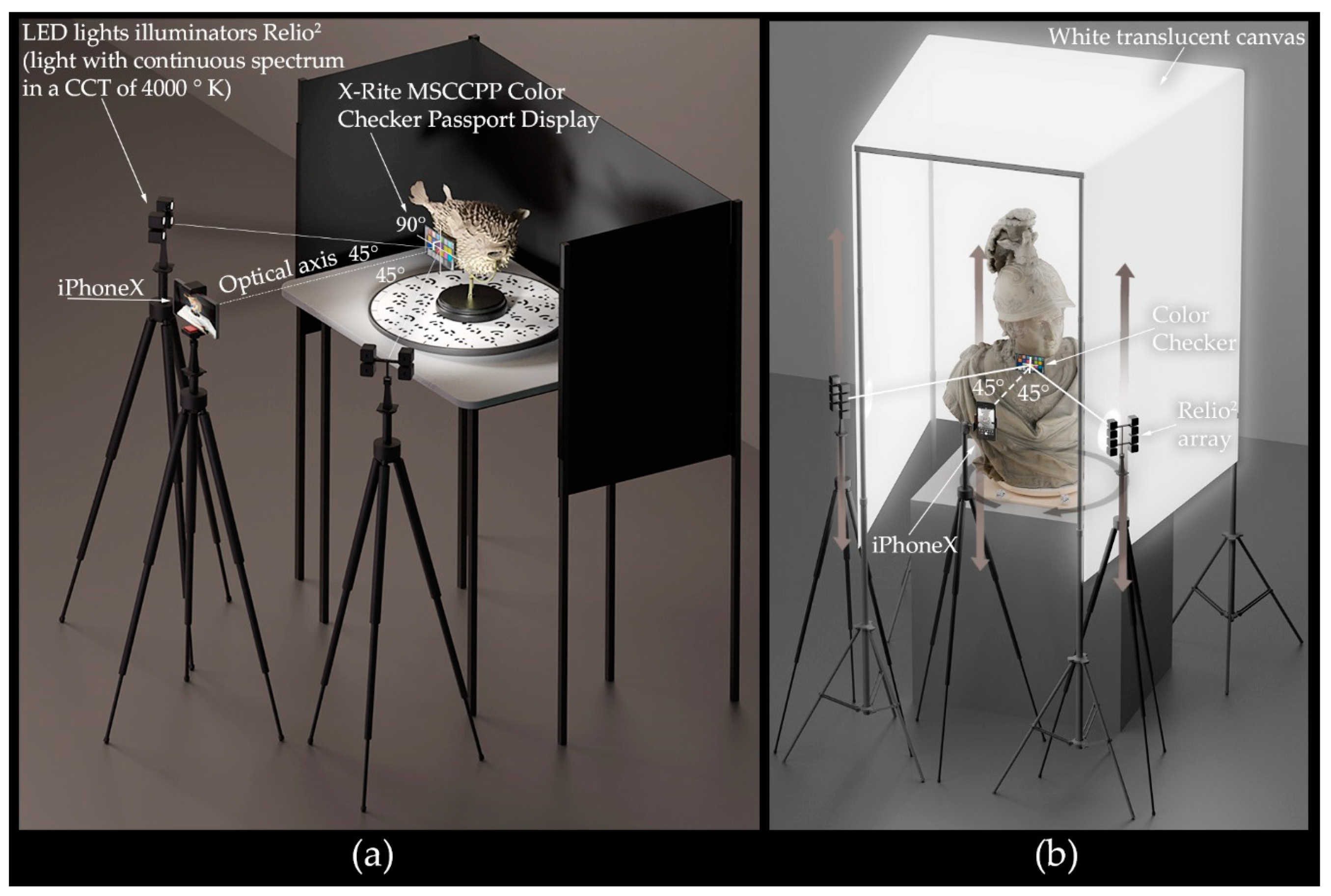
  • An illuminator kit to ensure controlled and high-quality light to get uniform, diffuse illumination. The illuminant was supplied by a series of Relio2 illumination devices [71], a very small lamp (35 × 35 × 35 mm, 80 g) emitting continuous spectrum light at a Correlated Color Temperature (CCT) of 4000 °K, a neutral white with high color rendering, a brightness of 40,000 lux at 0.25 m and a Color Rendering Index (CRI) > 95% with high color reliability on all wavelengths. It avoids the excessive emission of heat and harmful UV and IR radiation, which could damage the most fragile artefacts hosted in museums.
  • A color target ensuring the right color reproduction. We selected the smartphone-sized CCP to guarantee full compatibility with existing data of the ColorChecker Classic (X-Rite Inc., Grand Rapids, MI, USA) with dimensions fully appropriate with most of the objects collected in a small-medium museum.
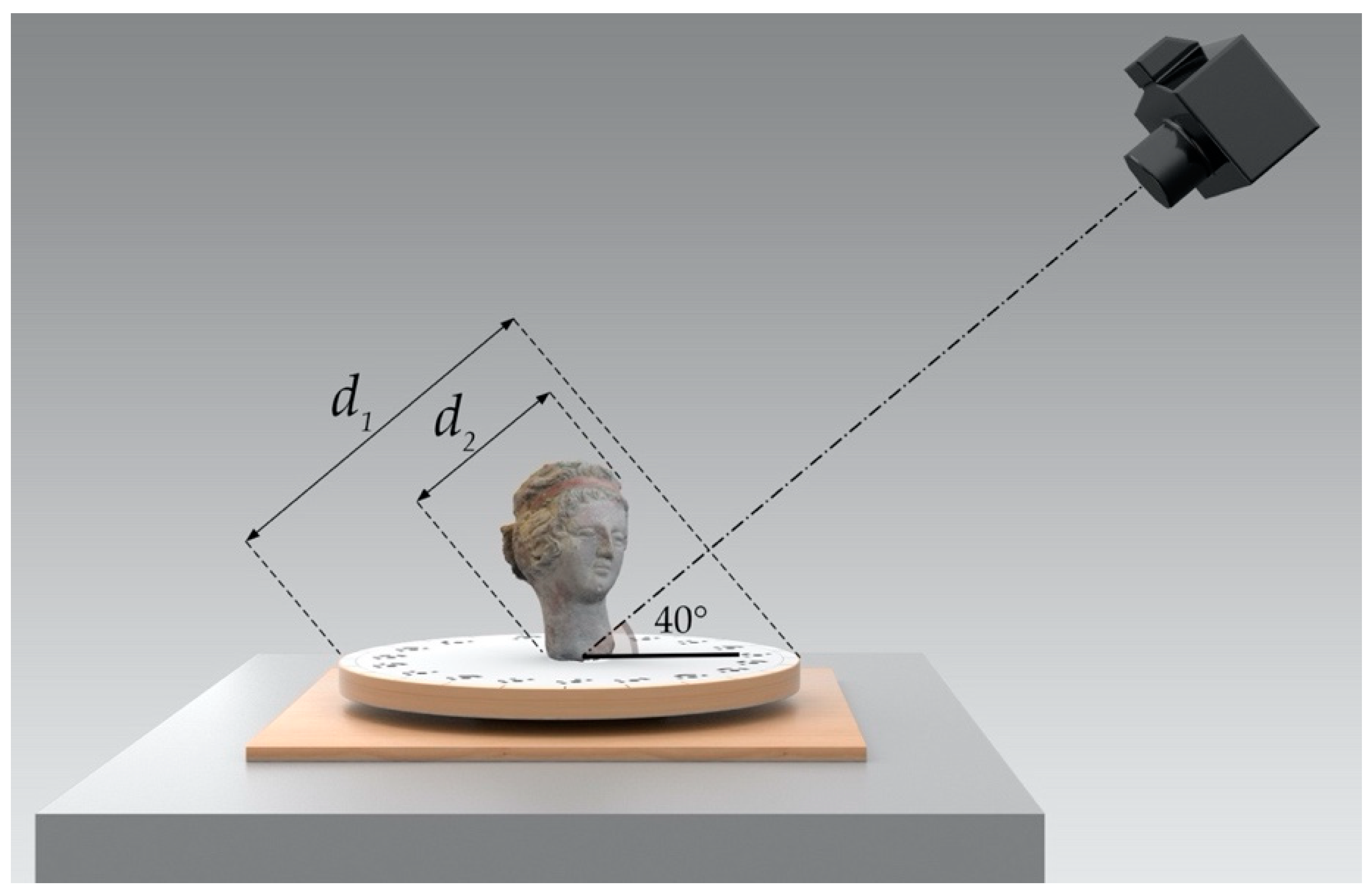
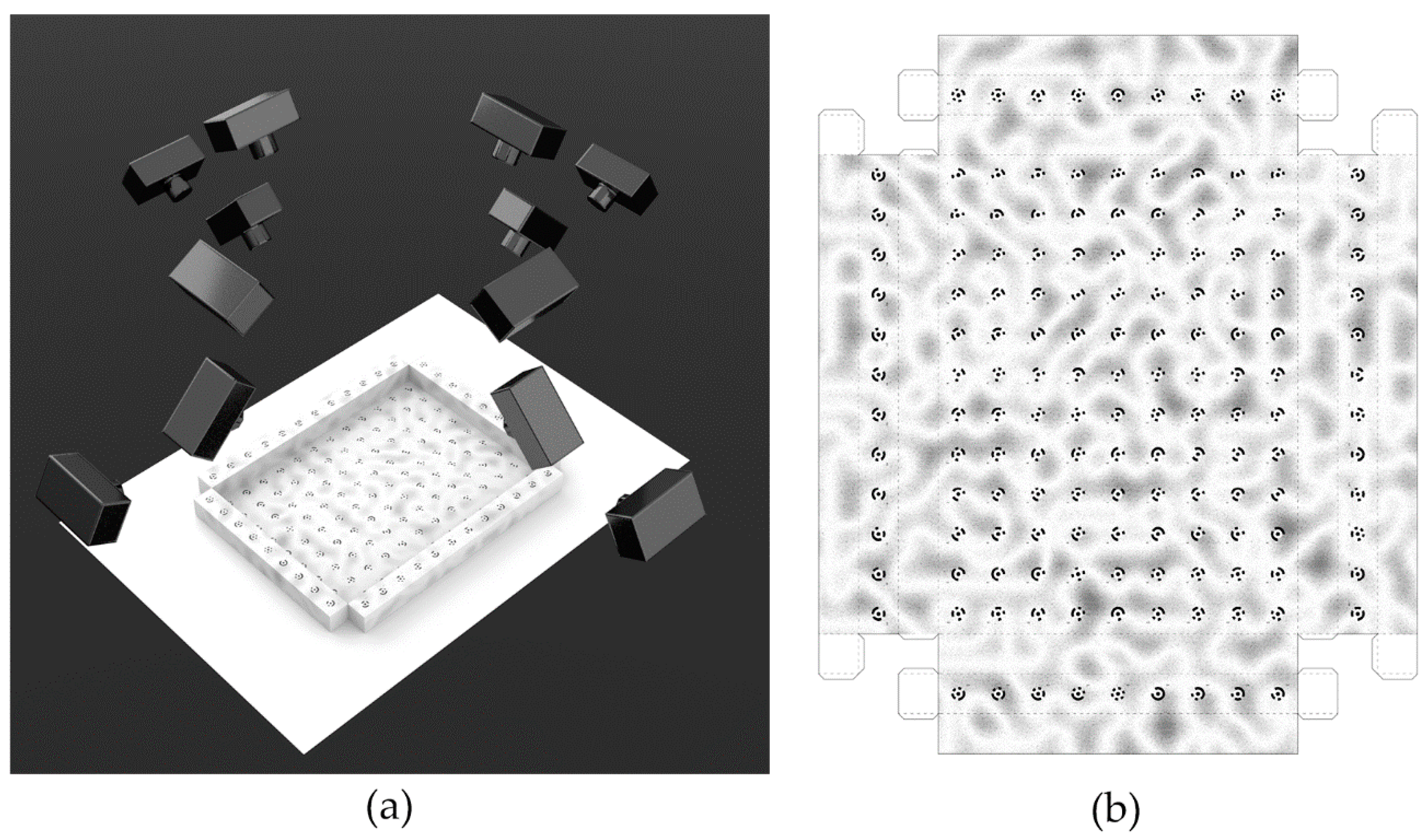
  • A rotating support with a set of Ringed Automatically Detected (RAD) coded target. They are both printed upon the circular flat surface hosting the artefact to be digitized, as well as on six regularly arranged cubes, textured with RAD targets to help alignment and scaling of photogrammetric models. These cubes are firmly connected to the rotating table profile by metal rods, radially placed along the circular plate’s thickness and rotating with it. We avoided solutions with stepper motors and controllers to drive the movement of the table as, for example, in [15], requiring too complex management, use and difficulties in the fabrication for CH operators. We preferred to prepare guidelines for a correct use instead. To address the mismatch problem between the limited, accurate, number of tie points belonging to the rotating table extracted by the software (i.e., the highly constrained by the RAD targets tie points) and the larger but less accurate, number of points extracted on the object, a procedural texture to the surface of the rotary table was applied. Its purpose is to fill large blank areas between the targets–poor in homologous points–and supply frame alignment process with a more balanced condition. According to the workflow we developed, some typical issues generated by the general use of camera parameters were addressed, such as the proper adjustment of the camera-object distance that produces a correct depth of field. Even though the process can be easily applied by users with average photographic skills, the common macro problems appear when taking pictures of close objects, mainly due to the adverse ratio between distance and focal length. To keep in focus all over the image frame the targets placed on the calibration plate, the aperture size was decreased to get an acceptable depth of field or it was reduced raising the camera elevation [72]. We addressed this problem in the guidelines where solutions and tricks are explained taking our case as an example. The iPhone X camera was used at an approximately 40° inclination and an object-to-camera distance of 620 mm. The aperture was set to f/1.8. The focal length was 4 mm and the sensor size is 4.92 mm. At an object-to-camera distance of 1100 mm, assuming a circle of confusion of 3 µm and applying the calculations detailed by [73], the depth-of-field will be 930 mm. Referring to Figure 4, the width of the sheet with the RAD targets is 348 mm, which, when viewed at a 40° angle, reduces to a depth of d1 = 348 cos(40°) = 266 mm. This would suggest that the depth-of-field is adequate for this application, especially given that the f/22 aperture would be expected to introduce diffraction blurring of approximately 10 µm.
  • A 3D test-field, formed by 150 RAD coded targets, using 12-bit length coordinates, which can be easily printed, using a 600-dpi b/w printer on rigid paper sheet, cut targets out and glue them (Figure 5). The coordinates for targets 1–108 were known, while targets on the edge of the frame were not given due to the difficult determination of the errors introduced by the paper thickness and construction problems. This shape will supply the photogrammetric application–used for the determination of the internal orientation–with a 3D point array since the shape of our objects is in general far from being flat.

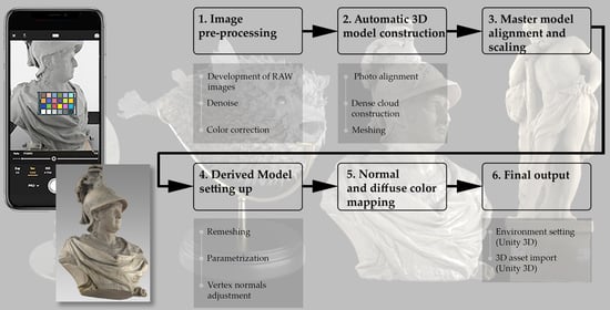
3.2. Workflow Overview

From the 3D model acquisition, construction and visualization perspective, the solution includes the three components described in the Section 1. From the operator’s point of view, it requires:
  • To place a CCP target in the scene;
  • To take photographs camera, using a predefined sequence network geometry;
  • To handle some script to automatically activate the different phases of the photogrammetric reconstruction, with only one extra-step to scale the 3D model (specifying measurements);
  • To import the model in the application template designed using Unity 3D environment.
The proposed workflow is a six steps process (Figure 6):
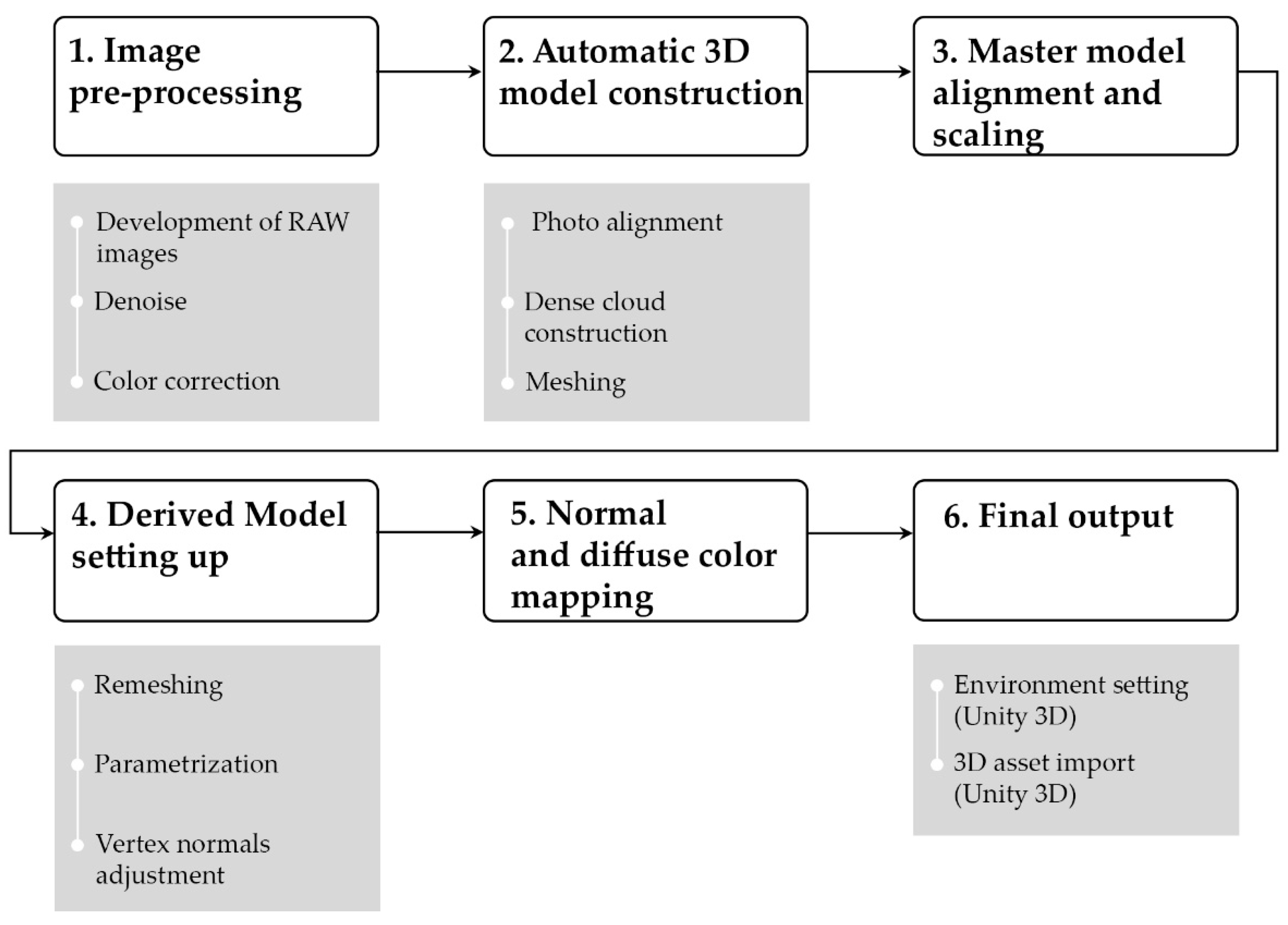
  • Images pre-processing: development of RAW images, denoise and color correction;
  • Automatic 3D model construction: photo alignment, dense cloud construction, meshing;
  • Master model alignment and scaling;
  • Derived Model setting up (remeshing, parametrization, vertex normals adjustment);
  • Normal and diffuse color mapping;
  • Setting the environment with Unity 3D and importing the 3D model.
The photogrammetric phase is characterized as follows:
  • Automated image pre-processing as in [74], aimed at enhancing photograph quality (radiometric calibrated images) yielding better results during the following image orientation and dense image matching;
  • Feature extraction and matching between images using our implementation of the ASIFT detector-descriptor [75] to ensure better matching between images [76];
  • Outliers filtering (incorrect matches removing), exploiting the Random Sample Consensus (RANSAC) algorithm [77] and a robust estimation of the acquisition geometry through linear models that impose geometric constraints;
  • Estimation of the parameters of the internal and external orientation. The approximate intrinsic parameters used in the essential matrix computation are obtained from the image EXIF tags. We then apply the Bundle Adjustment (BA) [78] in the variant implemented in the software used, a customized version of the open-source COLMAP [35,79];
  • Dense point cloud reconstruction, exploiting semi-global matching algorithms;
  • Dense point cloud interpolation, mesh reconstruction, mesh texture mapping and 3D model scale. This and the previous phases are based on a completely automated version of n-frames SURE, a state-of-the-art commercial software, designed to generate 3D spatial data [80] based on Semi Global Matching [81] and that can be implemented as a web-service. An open-source solution was also tested with minimal loss of quality. To scale the 3D model the user has just to place markers in two different photos in correspondence of the four-crosses mark placed on the CCP target corners. Distances among crosses are known, they are constant across different targets and accurately measured in laboratory on many samples. Using the rotating table, it is possible to take advantage of another solution: a simple. XML file with RAD coded target coordinates is imported in the reconstructed scene file.
At the end of the workflow, an extra step to get the derived models is possible. These are obtained by an isotropic quad-dominant re-meshing procedure [82]. This special type of simplified geometry guarantees a good fitting and better automatic and manual parameterization of the edge sequences to the features of the master models, ensuring greater consistency compared to more detailed triangular meshes.

3.3. Formal Characterization of the Acquired Objects

The work was organized starting from an analysis and a typological mapping of the possible artefacts under investigation, to identify the most representative case studies. The analyzed artefacts were therefore classified both from a typological and a geometric point of view and based on the quality of the surface and material properties. The aim was to evaluate the most appropriate methodology and tools depending on each case study. Some samples were chosen to provide a representative repertoire of museum artefacts based on the following parameters:
  • the formal and material characteristics of the artefact;
  • the recurrence of the formal and material peculiarities identified;
  • the tools and digital survey methods available and suitable;
  • the accessibility and consequent maneuverability of the artefact.
To evaluate and consequently to represent the proper level of complexity of the objects we define two main features divided into six categories (three per each one) able to identify tools, parameters and potential issues/criticalities in the workflow Table 1:
  • Extrinsic features
    Spatial distribution (SD) (Figure 7a–c) affects surveying activity. The most unfavorable scenario occurs when one dimension is prevailing on the other two (X ≃ Y << Z), followed by the case in which the distribution of the masses that form the object is two-dimensional (X ≃ Y >> Z);
    Topological complexity (TC) plays a crucial role since it affects every operation of the proposed workflow: when the object is not a simply connected space, for example, it presents through holes or even in case it has blind holes acquisition planning and further phases (parameterization, texturing, etc.) will be increasingly complex;
    Boundary conditions (BC): availability of surrounding working areas free from obstacles.
  • Intrinsic features
    D/d ratio: where D is the diagonal length of the bounding box containing a piece of a collection and d is the average length distance among vertices, namely the model resolution. The higher this value the greater the complexity of the survey as high detail on a large object is required (Figure 7, right);
    Surface characteristics: minimal surface detail rendered, surface and textural properties, different reflectance behavior (e.g., Lambertian, specular dielectric, translucent, transparent surface, etc.);
    Cavity ratio (CR) is a parameter that qualifies the impossibility of digital acquisition for some parts of the surveyed object. It depends on the surveying technique and on the adopted device; it is given by the ratio between D and W, where D is the depth and W is the hole width. For values between 0 and 1 the planning of the survey is simple, but it is progressively more complicated for values greater than 1 (Figure 7e,f).
Relating to the size of the surface irregularities, thresholds were defined to adopt the most appropriate geometric modeling methods or to simulate the irregularities using graphic effects. For surface irregularities ranging in size between about 0.1 and 1 mm, the detail can be rendered through graphic effects (i.e., normal mapping) while, for irregularities greater than about 1 mm we modeled in 3D the proper shape of the artefact. These classifications allowed to define features of ‘Master Model’ and ‘Derived Models’ for various classes of objects.

3.4. Authoring Environment for Interactive RTR Visualization

To produce faithful realistic 3D models, replicating the whole spectrum of the light-surface interaction, we conceived a multi-staged pipeline system as follows:
  • Step 1. Materials’ appearance reproduction;
  • Step 2. RTR visualization development with accurate color reproduction on a 100% sRGB capable display using an RTR engine running on multiple devices;
  • Step 3. Production of a visualization and navigation graphic interface based on common gestures.
Materials macrostructure and mesostructured features are reproduced by the mesh geometry in the ‘Master model,’ embedding into the mesh the low-frequency geometric details and using the normal map rendering approach for the high-frequency ones in the ‘Derivatives models.’ This separation of high-frequency geometric detail from the low-frequency one allows a better geometry estimation including features such as self-shadowing or parallax deformation at macrostructure.
Microstructure behavior is addressed developing a superset of many shaders able to correctly reproduce the light-material interaction of a lot of materials which the museum objects are made of. This approach avoids to re-design the shader each time. Four types of maps (diffuse, normal, height and glossiness) modulate the different parameters. The implementation of the multitexture technique consists in a constrained parameterization, based on an iterative routine. It allows users to keep under control texel density of reprojected frames upon the (u,v) parameter space [83], as well as the level of consistency among 2D charts and corresponding 3D areas on the mesh. This process leads to significant benefits, including better and more intuitive interactions between the set of textures applied to the model and the applications dedicated to the light-matter relationship.
Many software frameworks support these features. Between these applications we selected those supporting cross-platform deployment and visualization, the use by non-expert operators, low-cost, high render quality and the ability to allow an easy, customized exploration of artefacts at many scales (i.e., the typical requirements of museums’ visitors, art scholars and restorers).
We opted to use a staged render sequence implemented into the Unity 3D RTR engine. Unity 3D is a game development platform consisting of a Graphical User Interface (GUI) and a game engine that can be adopted to author several interactive simulations, ranging from small mobile and browser-based games to high-budget applications and AR/VR experiences.
To improve Unity’s output visualization quality, we developed and improved features relying on our specific requirements, to ensure precise conformity to:
  • light, with its actual spectral composition in rendered models;
  • color, with an accurate simulation to mimic material appearance under different light directions;
  • surface, with precise replica at different scales of the object’s surface.

4. Image Pre-Processing

To correctly solve problems related to image noise and color correction we developed an automated image pre-processing technique from RAW imagery, starting from our previous solution described in Ballabeni et al. [84].

4.1. Raw Image Reconstruction

The Apple iPhone X supports, as most of the smartphone cameras, RAW format through the Adobe Digital Negative (DNG), a patented, open, non-free lossless format based on the TIFF/EP standard format, that could be adopted both as a RAW file format and as a ‘non-RAW,’ with partly processed images with the application (e.g., of white balance and of a camera color profile). This second implementation is adopted by all the smartphones makers, as evident in the Apple iPhone X, where metadata reports the inclusion of the camera profile using the Apple Display P3 color space. Moreover, some other non-transparent processes could be embedded as ‘hidden’ in the DNG file avoiding the conditions of an efficient image pre-processing, that is, to retains only the basic in-camera processing (black point subtraction; bad pixel removal; dark frame, bias subtraction and flat-field correction; green channel equilibrium correction; Bayer interpolation).
To minimize these unwanted modifications, we customized the processing software to restore the original file state using the software described in [85]. We removed the color profile, the automatic denoise and the camera image crop.

4.2. Image Denoise

To fulfil noise reduction requirements in the photogrammetric field, we developed a denoise process integrated into the demosaicking and color correction process.
The denoise phase include both the noise measurement and the denoise inferred by previous measurements steps.
For the noise measurements, we used a procedure in which it is measured in the XYZ linear color space using the six greyscale patches of the CCP, converted to 1–255 in the RGB color space and, finally, normalized to White–Black (Patches A4–F4) pixel level:
100% × (Noise in pixels)/(A4 patch pixel level–F4 patch pixel level).
This technique involves fewer measurements and less complex calculations of the ISO and IEEE standards but it is accurate enough, while it references the noise to the scene: noise performance is not affected by camera contrast, allowing the accurate identification of the algorithm parameters necessary to enable our denoise.
For the denoise phase we used an improvement of our solution named CBM3D-new presented in [76], to which we refer for details. This denoiser is basically a variant of the state-of-the-art Block Matching 3D (BM3D) filter, combining the principles of nonlocal denoising with transform-based denoising algorithms to exploit the mutual similarity between patches at different locations in the image [86,87]. In detail, the new implementation consists in the implementation of three different parameters profiles corresponding to different SNR.
This solution is more traditional than modern denoising methods that employ neural networks to learn the mapping from noisy images to noise-free images. Deep learning can represent complex image and noise properties, but the training of these models requires large paired datasets. Despite significant work on designing neural networks for denoising, recent benchmarks [88] reveal that deep learning models are often outperformed by traditional, hand-engineered algorithms when evaluated on real noisy RAW images captured from real.

4.3. Color Correction

The developed target-based CC solution include:
  • a physical reference chart acquired under the current illumination (corresponding to the illumination to be discarded), in our case the described (see Section 2.5.2) CCP;
  • a color space reference with the ideal data values for the chart patches. In our case ideal data values are the 8-bit measured by Denny Pascale [89] for targets built before the end of 2014 and the X-Rite reference values [90] for targets built after the end of 2014, to skip, with a minimum loss, a complicated spectrometric measurement. The color space used is the common, device independent CIEXYZ [91];
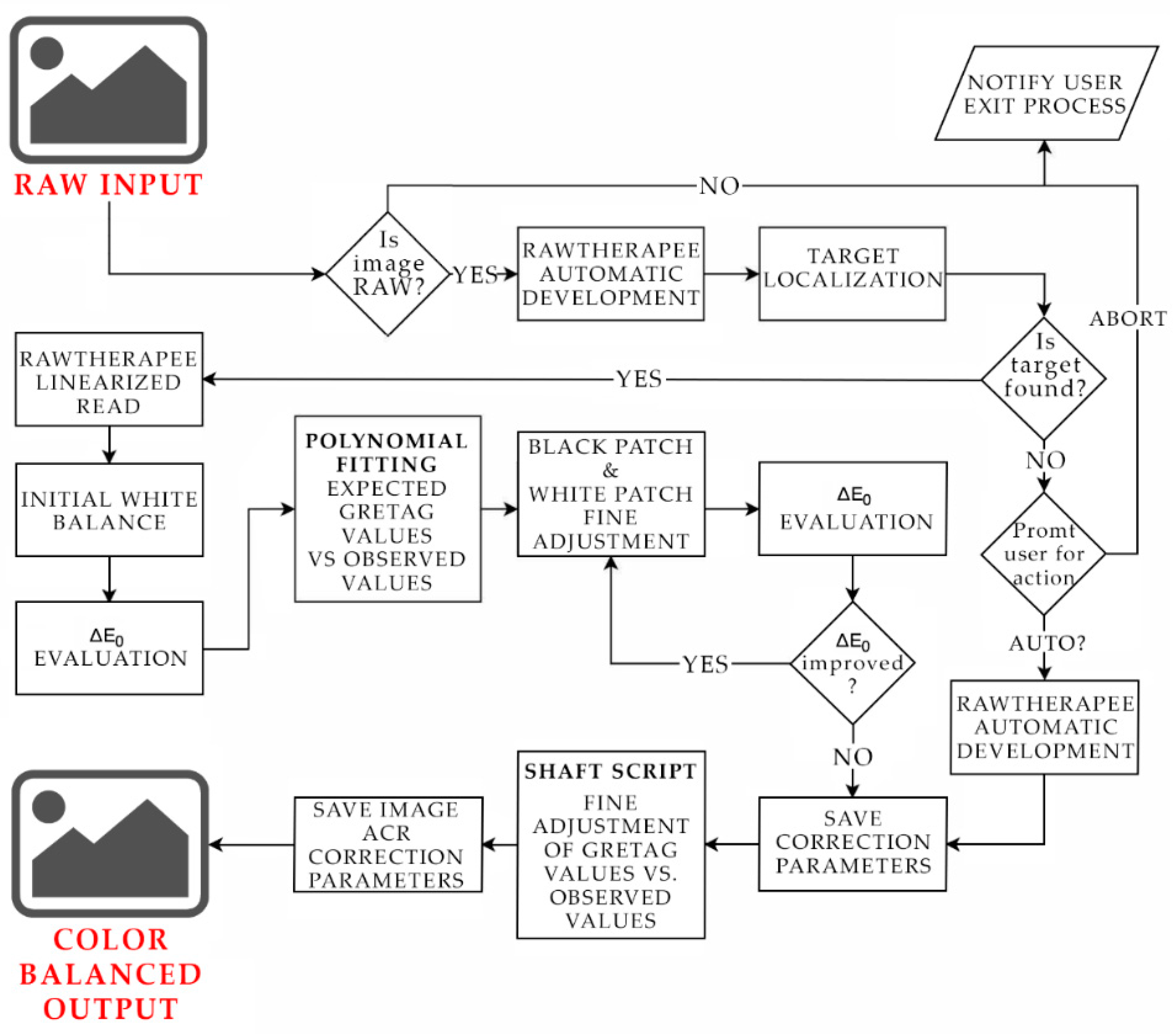
  • a way to relate or to convert the device color space to the reference color space chart. This step in our solution is based on the SHAFT (Saturation & Hue Adaptive Fine Tuning) [92], a software for target-based CC supported by RawTherapee [93]. SHAFT exploits a set of optimization and enhancement techniques on exposure, contrast, white balance, hue and saturation and is based on the linear CC for successive approximations approach. SHAFT can recognize the target on the image allowing a completely automated process. To avoid its main limitation (i.e., the use on original highly incorrect images, with high color dominant, could fail) SHAFT is coupled with a polynomial regression correction [94] (Figure 8). In the present case the SHAFT was adapted, embedding appropriate tests before the processing, to identify possible inconsistencies in the images depending from specific smartphone cameras features: (1) the today’s emphasis that manufacturers give to the amplification of color saturation, to have a better color perception on the small smartphone screen, with an incidence that, in the case of Apple Display P3 can reach up to 10%; and (2) the exposure correction by the gain that can limit a faithful color reproduction in the case of images too dark corrected hiddenly.
  • a way to measure and show errors in the device’s rendering of the reference chart. We used the CIEDE2000 [95] color difference metrics acknowledged as colorimetry standards by ISO and recommended by the Commission Internationale de l’Éclairage (CIE) [96] for color differences within the range 0–5 CIELAB units [97]. The formula computes color accuracy in terms of the mean camera chroma relative to the mean ideal chroma. The equation is, in practice, the Euclidean distance in L*a*b* color space between captured image values and measured values with some correction factors and is recommended by CIE mainly and compensates using coefficients for perceptual non-uniformities of the L*a*b* color space and thus correlates better with perceptual color difference than earlier equations [98];
  • an output color space. We selected the rendered space IEC 61966-2-1 sRGB, the today default color space for multimedia application [99], allowing consistent color reproduction across different media and full support of 3D API graphics used (Microsoft Direct X by Microsoft Corp., Redmond, Washington, USA and Apple Metal, by Apple Inc., Cupertino, CA, USA). Its potential issues (non-linearity, smaller amplitude of the human perceived color space) affect a little the quality of rendering also because it can represent all the colors displayable on a today prosumer monitor, that is the target of this project.

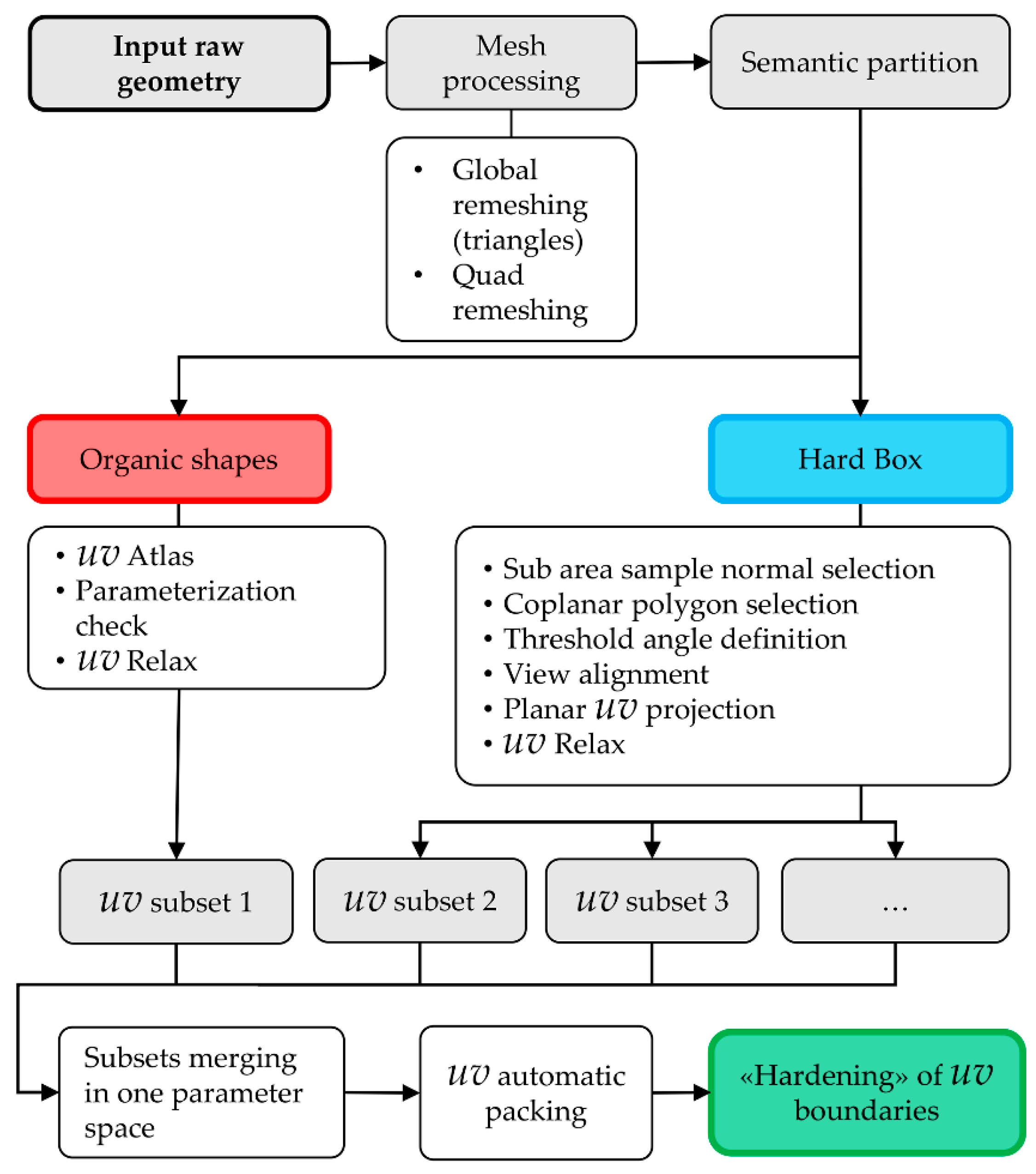
5. Geometry Processing

Geometry processing consists of a two-stage process to solve two different problems:
  • the quality of the acquired mesh geometry, which using smartphones is usually noisy, could present artefacts and could generate irregularities in the subsequent texture mapping;
  • the need to have a visually faithful but lightweight 3D model to be used on low-end hardware in the museums or on the go.
The first step of the geometry processing is the mesh post-processing aiming, on the one hand, to minimize mesh flaws and generate a proper mesh filling to achieve efficiency of the texture mapping parametrization and on the other hand the mesh complexity in terms of number of vertices, the regularity of the connectivity, the quality of the triangle shape and the sample distribution on the surface. This is followed by a triangles-to-quad-dominant mesh conversion.
The second step consists of a parameterization and baking (render-to-texture) procedure to generate a lighter geometry supported by a normal map meant to return the mesoscale details.

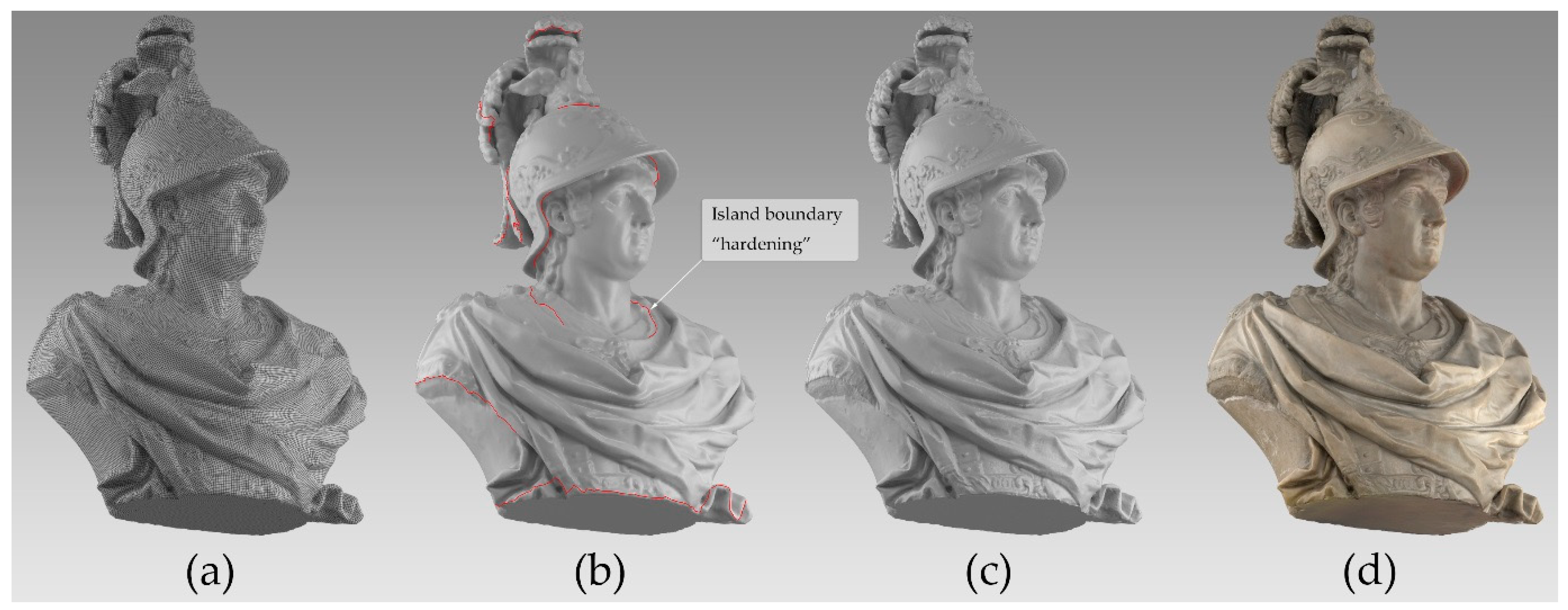
5.1. Mesh Post-Processing

The mesh processing phase starts with the mesh quality enhancement from the photogrammetric pipeline, achieved introducing in our workflow a remeshing step. This operation produces a new triangular mesh with an adaptive vertex distribution, isotropic sampling and almost equilateral triangles. The solution relies on the extension by Botsch and Kobbelt [100] of the technique described by Dunyach et al. [101]. The algorithm takes a target edge length as an input and then repeatedly splits long edges, collapses short edges and relocates vertices until all edges approximately reach the desired target length. Few simple rules are enough to grant that the remeshing algorithm will preserve the input model features. Maximal and minimal edge length of the output mesh and a maximal distance to the original mesh are predefined following typical features of sculptures (edge length 0.1–1 mm; max distance 0.05 mm). The result achieved by the remeshing process is a new mesh that is curvature-adaptive and regular.
The second step of the post-processing phase aims to produce a low-resolution mesh involving the combination of decimation techniques and the conversion to quad-dominant meshes.
Mesh decimation is made using reduction criteria illustrated in Section 2.3 and specifically the D/d ratio. The polygon count of the low-resolution mesh is the result of a series of consideration based on the level of proximity and the quality of the perception that the final user needs to reach inside the interactive application the asset is designed for.
The aims and the technique used for the triangle-to-quad dominant meshes could be better illustrated by a typical use case that was provided by the Porcupinefish in the SMA’s collection (one of our test objects). It discloses a shape overall relatively simple but extremely complex locally, due to its tiny details (Figure 9a,b). Small sequences of spikes with different lengths, aligned to the global shape, cover most of the creature’s skin. To keep as high as possible the frame rate of its interactive visualization, it is necessary to lower the number of displayed polygons. The use of an automatic (Figure 9c) or manual (Figure 9d) simplification process implies the need of punctual retouches carried out with manual polygonal modelling techniques, particularly on the tips of the spines, which tend to lose consistency and change their lengths by a progressive introduction of dangling faces in place of their very pointed ends (Figure 10). To solve this problem, we used a variant of the quad-dominant isotropic remesh [82] allowing excellent compromises to the problem of the minimal deviation in low-resolution model compared to the master model. We tabulated remeshing parameters using as a reference the Edge Average Length (EAL) of a model and a threshold related to the type of the object and model used, following the classification in Section 2.3. This value also defines the level of accuracy of the normal map that will store the mesoscale features lost in the remeshing process. The higher is EAL, the higher is the deviation between the master model and the inferred ones. Therefore, a greater number of details will have to be stored at normal-map level.

5.2. Mesh Parameterization and Normal Mapping

A normal map is generated using 3D modeling and baking from high-poly geometry to a low-poly geometry technique to visualize a mesostructure visually analogous in quality to the explicitly modelled one but using a lighter polygonal model (Figure 11). The baking process is based on a series of geometric considerations shown in detail on a 2D section of the model in Figure 12. The resolution of this texture is a compromise solution obtained by balancing three factors: the number of normals in the high-poly (i.e., number of vertices), the parameterization quality (texel density) and the next higher power of two corresponding to a pixel area equal to the number of vertices. A crucial parameter is the maximum distance ( Δ max ) in absolute value between high-poly and low-poly (Figure 12). In our case it depends on the minimum feature and the size of the object (see Section 2.3).
In detail, our implementation of the per-pixel tangent space normal maps was achieved focusing and giving solution to three main problems potentially generating various types of issues:
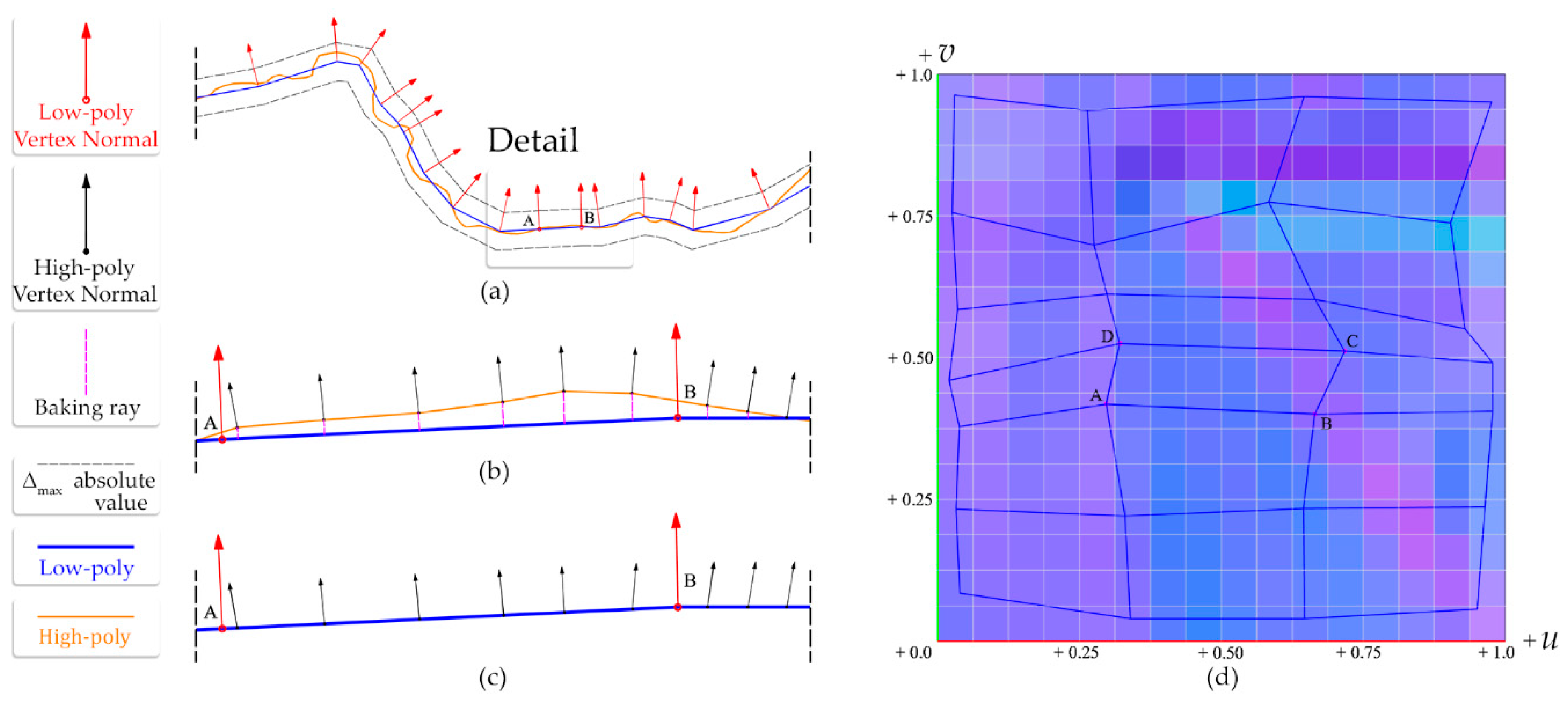
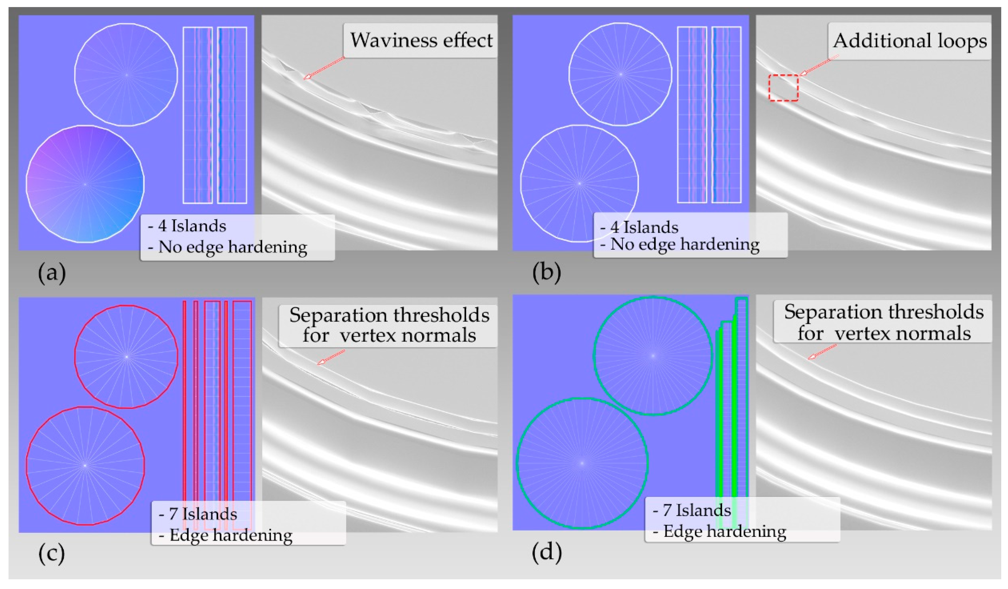
  • Correct size of the texture determination. The low-poly mesh must be parameterized considering two aspects: keep as low as possible the number of islands and to have a correct texel density, necessary to get rid of over-detailed or under-detailed areas relative to the rest of the rendered scene. As the best parameterization has a size that occupies the parameter space the inequation to evaluate the proper resolution of the normal map is the following:
    A n 2 2 n 100 F r ,
    where A n is the number of vertex normals, F r is the fill rate and 22n is the area in pixels resulting from a number two power usually used as a texture size. We implemented this inequation at the top of the baking process. An example is in Figure 13.
  • Smoothing groups and “Mikktspace” implementation. To accurately control normals behavior we adopted a solution very common in the game industry, the so-called “Mikktspace,” which calculates normal maps in tangent space [102] joint with the use of the smoothing group technique:
    • the “Mikktspace” technique prevents problems linked to (a) the math error which occurs from the usual mismatch between the normal map baker and the pixel shader used for rendering, resulting in shading seams (i.e., unwanted hard edges which become visible when the model is lit/shaded); (b) order-dependencies which can result in different tangent spaces depending on which order faces are given in or the order of vertices to a face;
    • by identifying the polygons in a mesh that should appear to be smoothly connected, smoothing groups allow 3D modeling software to estimate the surface normal at any point on the mesh and by averaging the vertex normals in the mesh data that describes the mesh, allow to have both hard edges and soft edges.
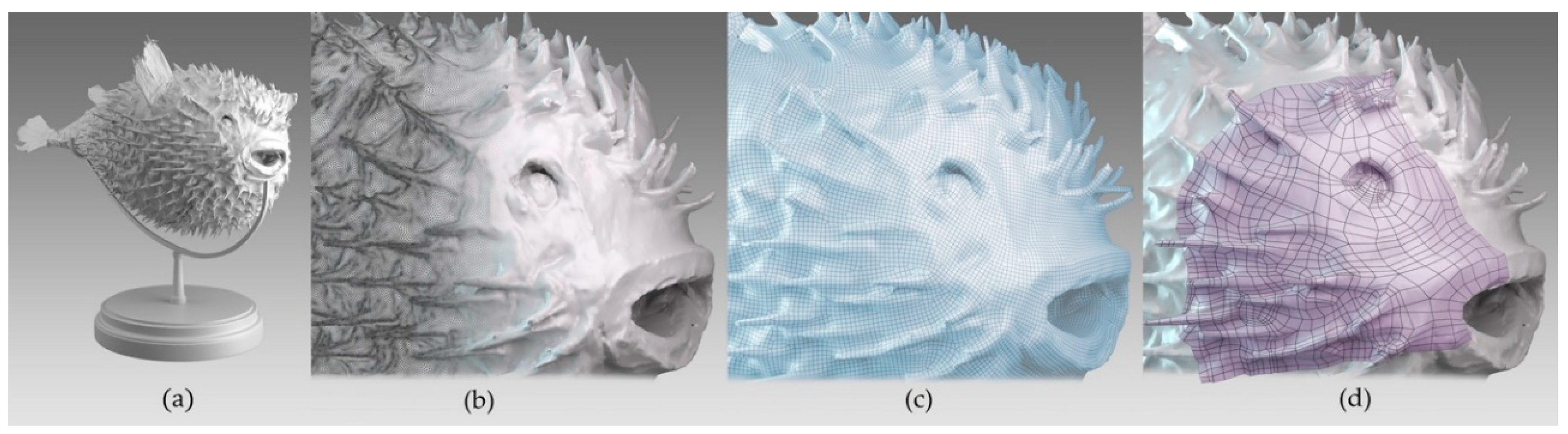
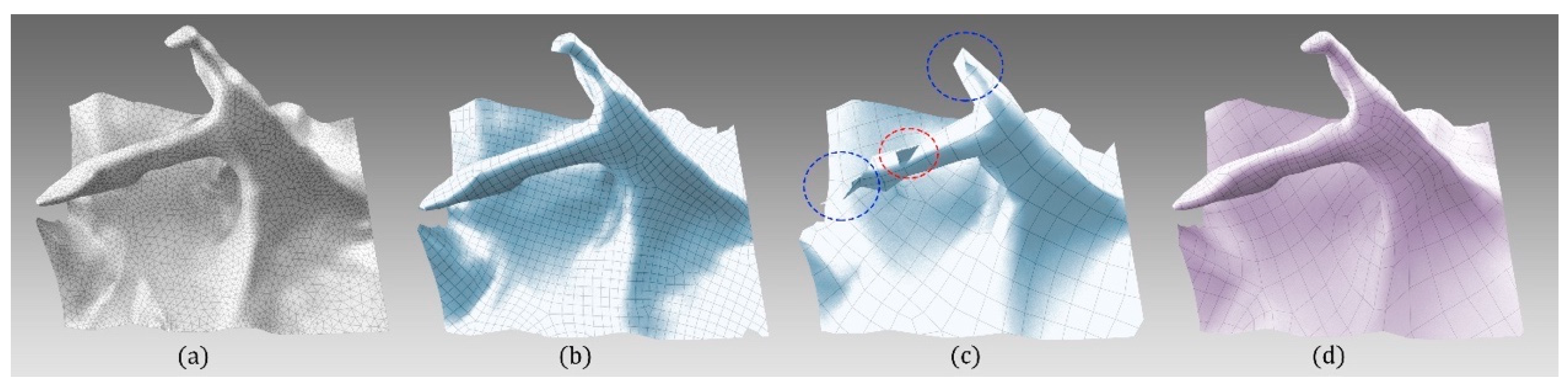
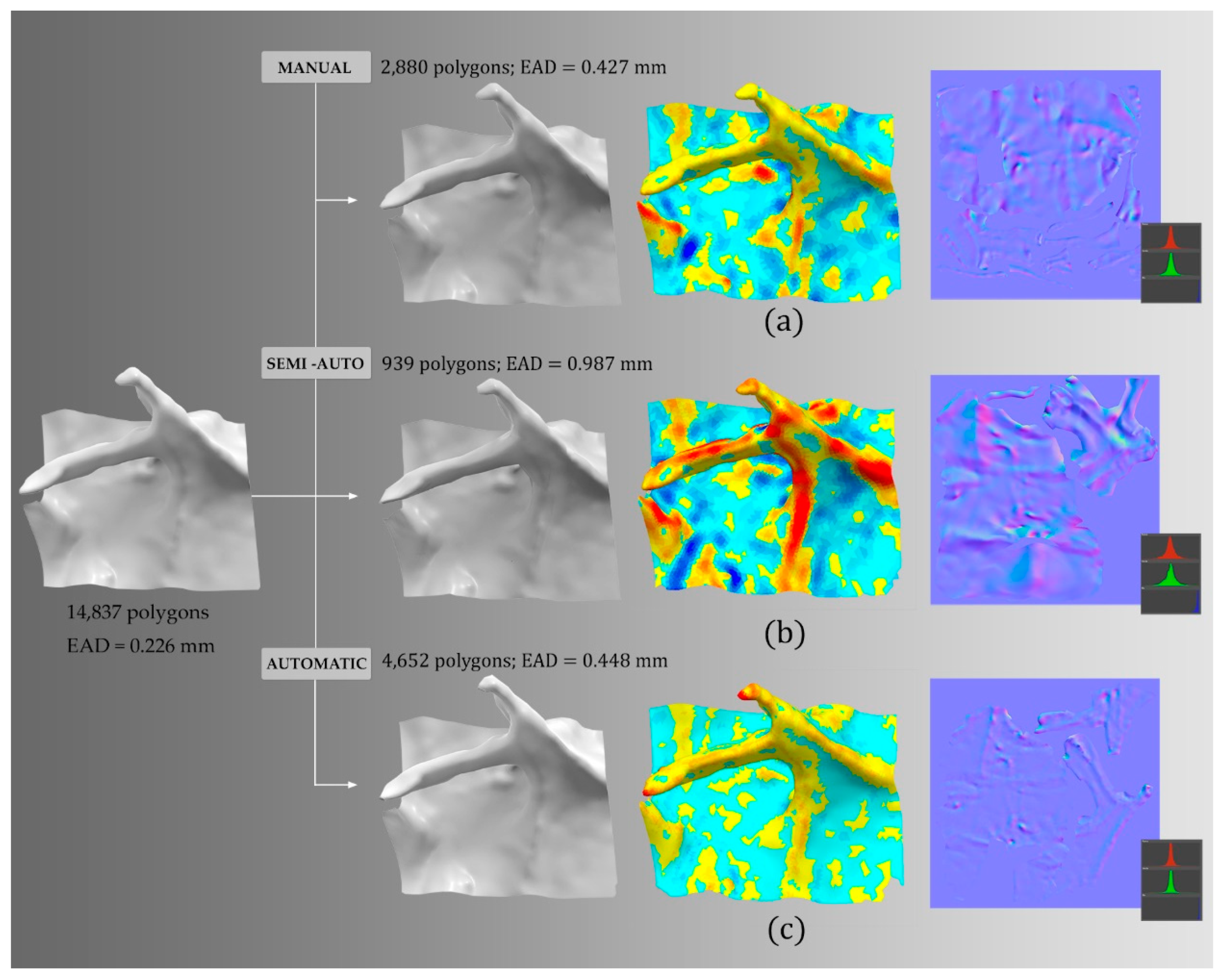
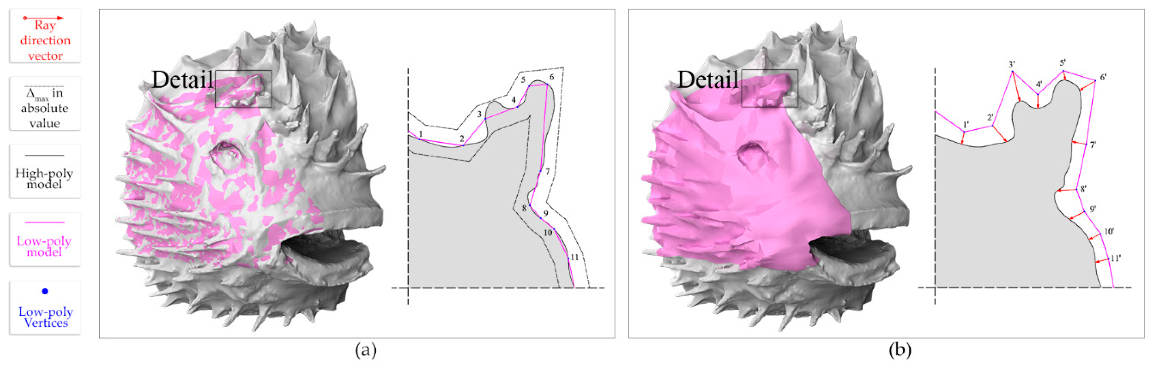
  • Errors in the normal map generation due to misinterpretation of geometry and topology corrections. Using automatic/manual/semi-automatic reduction techniques starting from a high-poly model open the way to a series of cases: sometimes diseconomies are generated in the production of the models or the normal maps are useless or further cases marked by a strong reduction in the number of polygons potentially generate more shading errors. (Figure 14a–c). Currently four solutions allow to solve problems such as:
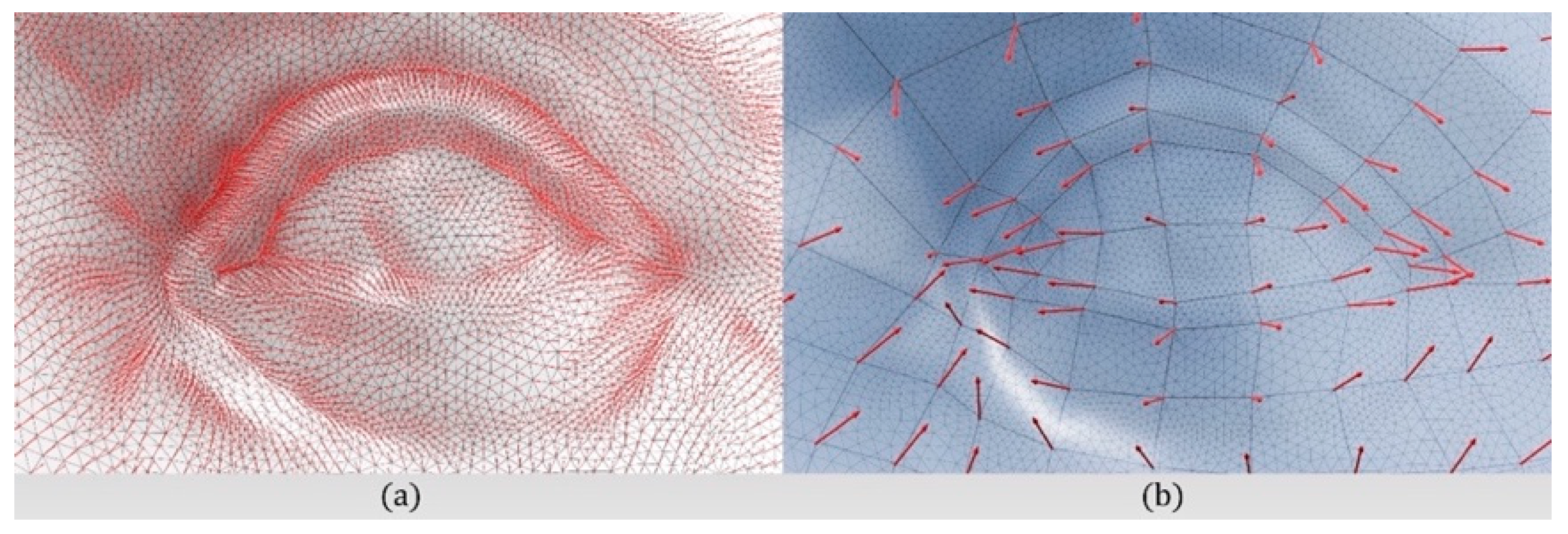
    • the use of a ‘cage’ (or projection cage) providing the low-poly model with better vertex normals flow, that is, saving in the low-poly model an alternative version, generally produced by an offset, then manually arranged in certain regions and stored as a morph (Figure 15);
    • the adaptive triangulation of quadrangular polygons before baking [103];
    • the introduction of additional loops of quad-polygons in the proximity of curved sequences of edges to reduce ‘waviness’ effect on cylindrical and bent surfaces (Figure 16);
    • the calculation of the normal map at twice the resolution strictly necessary (as stated by the Nyquist-Shannon theorem) and then downsampling at 50% of the size.
We developed an automated approach that exploits all the above solutions managing each problem with an appropriate technique (Figure 17). Starting from a high detail mesh, after the automatic modelling steps (global remeshing and quad-remeshing) is added a semantic partition that separates distinct types of shapes (organic and artificial/geometric) since they require different treatments on parameterization criteria.
While organic shapes can be parameterized with automatic systems in a single solution, surfaces shaped through the combination of regular geometric primitives must be split into subsets characterized by similar normals orientation: each subset needs a specific parameterization. Then individual fragments are merged into a (u,v) single map. Then, to each connected sequence of edges defining islands’ boundaries, a vertex normal is created, namely, a ‘hardening’ process is carried out affecting the shading by creating sharp creases along edges, able to enhance the baking solution. Finally, the normal map is calculated at twice the resolution necessary and then downsampled to 50% of the size.

6. Assessment of the Proposed Workflow

For the assessment of the proposed methodology, we selected specific (i) case studies able to cover most part of the problems of small-medium museums objects, (ii) acquisition equipment, (iii) complementary procedures able to verify the correctness of the developed workflow.

6.1. Case Studies

A set of heterogeneous objects were chosen from the Sistema Museale di Ateneo (SMA, Bologna, Italy) of the University of Bologna hosted inside Palazzo Poggi. These objects were useful to set up a procedure focused on the reliable and consistent acquisition of ‘micro’ and ‘meso’ details. The museum hosts various collections dedicated to geography and nautical sciences, military architecture collected by Luigi Ferdinando Marsili (Figure 18), physics, natural history, chemistry, human anatomy, along with the collection of fossils and dissected animals gathered by the naturalist Ulisse Aldrovandi.
SMA’s case studies were selected according to their variety and representativeness, following the classification criteria reported in Section 2.3 (Figure 19), that is, they consider the intrinsic and extrinsic features (Table 2). The acquired datasets correspond to four artefacts:
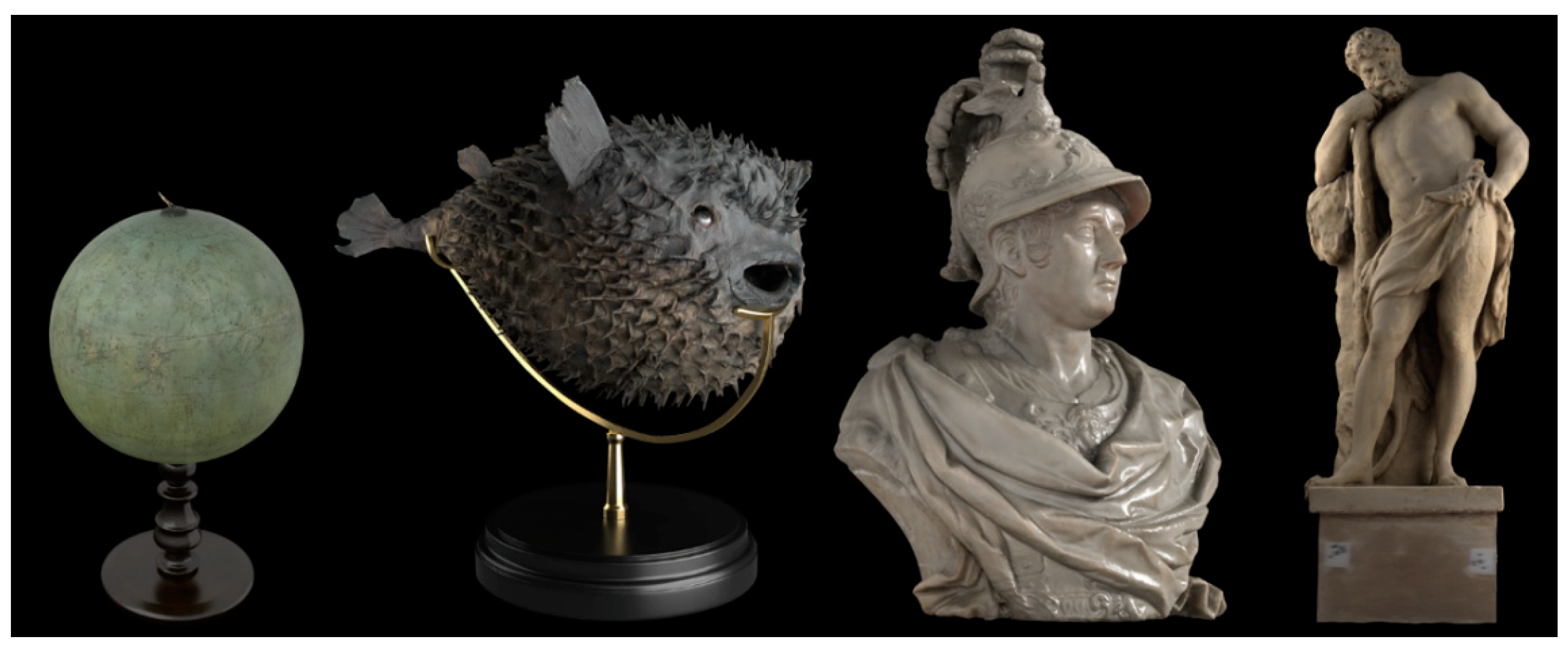
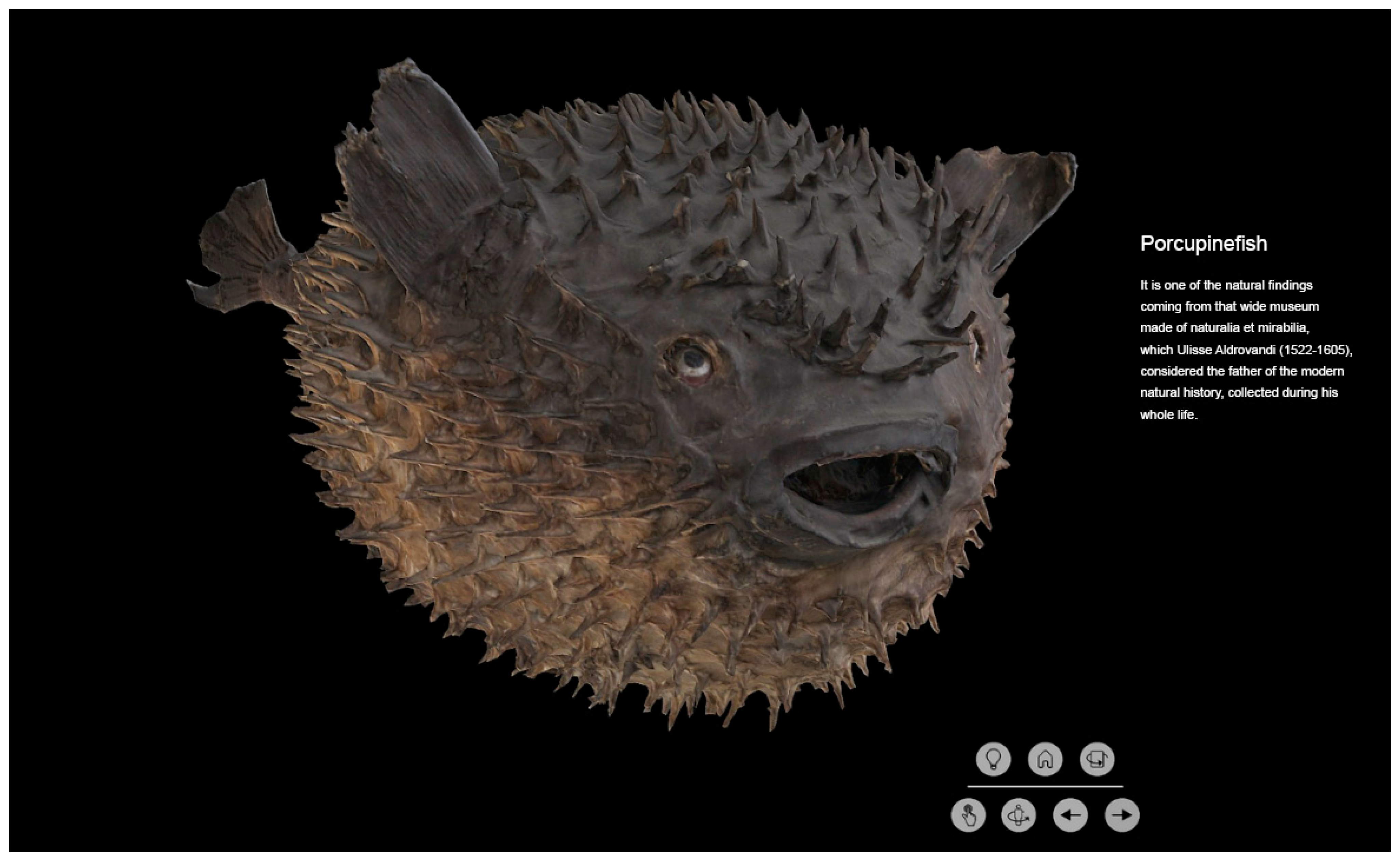
  • A Porcupinefish (Diodon Antennatus) undergone to complete taxidermy treatment: bounding box = 35 × 19 × 25 cm, highly specular skin and tiny details (Figure 20a).
  • A Globe by astronomer Horn d’Arturo: bounding box = 31 × 31 × 46 cm, highly reflective regular surface with a considerable Fresnel effect (Figure 20b).
  • A bust of the scientist, military, geologist Luigi Ferdinando Marsili (1658–1730): bounding box = 41 × 67 × 99 cm, made in Carrara marble a highly translucent, non-homogeneous material at the scale of the measurement process (Figure 20c).
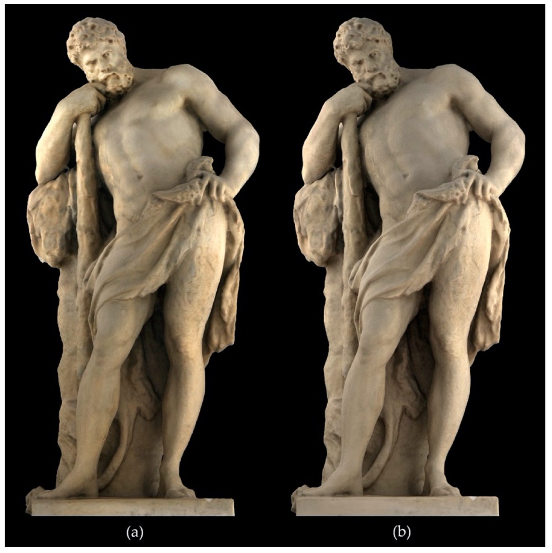
  • A statue representing Hercules (bounding box = 100 × 90 × 275 cm, made in sandstone). Due to its size and its exhibition conditions (Figure 20d).

6.2. Devices, Equipment Used and Acquisition Setup

Besides hardware (camera, lights, tripods, rotating table) and software described in Section 2, the evaluation of the shape complexity and geometric accuracy of 3D models obtained by smartphone was carried out adopting the following equipment:
  • Nikon D5200 SLR camera featuring 16.2 million effective pixels equipped with an f = 18 mm focal length lens during the acquisition. Remaining technical features of this camera and the Apple iPhone X camera are in Table 3.
  • Two Terrestrial Laser Scanners (TLS) with different characteristics to better measure the features of the different objects digitized:
    Faro Focus X 130 (Faro Technologies Inc., Lake Mary, FL, USA) with measurement range between 0.6 m and 130 m, measurement speed of 122,000–976,000 points/s, 3D point accuracy of ±2 mm at 10 m;
    NextEngine 2020i (NextEngine Inc., Santa Monica, CA, USA) with operational field of 342.9 × 256.54 mm (wide lens), measurement speed of 50,000 points/s, resolution of 0.149 mm, 3D point accuracy of ±0.3 mm.
Since the experimentations aimed at testing the effectiveness of the workflow for different cases, other devices were used. Table 4 schematically lists the tools used in each case study:
  • graduated rotating table with RAD coded targets with known spatial coordinates applied;
  • static lighting set consisting of two groups of four Relio2 (Montirone (BS), Italy) illuminators oriented respectively at an angle of ±45° towards the optical axis of the camera;
  • dynamic lighting set (mounted on telescopic arms with the possibility of panning and tilting) consisting of two groups of eight Relio2 illuminators oriented at ±45° with respect to the optical axes of the camera (Figure 3). This second array of lights enables different positions and orientations with respect to the object and better approximates a lighting panel;
  • resizable box structure to host objects to be captured, consisting of translucent white walls suitable to diffuse the light coming from the Relio2 illuminator array;
  • curtain made of black matte surfaces to mitigate the Fresnel effect on contours of reflective materials.
Using the rotating table, the objects were photographed by rotating it by angle intervals of 10°, thus simulating a circular camera network as the camera was moving around the object. To photographically cover the whole object, the camera was placed at different heights (i.e., 6 heights in the case of the Porcupinefish and the Globe and 8 heights for the bust), a procedure commonly used in photogrammetry when dealing with rotationally symmetric objects like globes or cylindrical seals. The number of photos and revolutions using the rotating table are shown in Table 5.

6.3. Camera Calibration Procedure

The first step in the photogrammetric data processing is the camera geometric calibration, to determine both the interior and the exterior orientation parameters, as well as the additional values. The most common set of additional parameters employed to compensate for systematic errors in digital cameras is the 8-term ‘physical’ model originally formulated by Brown [104]. The Brown’s model includes the 3D position of the perspective center in image space (principal distance and principal point), as well as the three coefficients for radial and two for decentering distortion. The model can be extended by two further parameters to account for affinity and shear within the sensor system. However, we skipped these parameters concerning levels of accuracy of one order of magnitude above the one required. The iPhone X camera calibration was carried out using the developed 3D test-field. A set of 20 images were captured using a tripod and a photo studio illumination set. It includes a set of convergent images (some of them rotated by 90°) with good intersection angles of rays from camera to the test-field [105,106].
The calibration process was calculated two times using different techniques:
  • Self-calibration in COLMAP. By default, COLMAP tries to refine the intrinsic camera parameters (except principal point) automatically during the reconstruction. In SfM, if enough images are in the dataset and the intrinsic camera parameters between multiple images can be shared, these parameters should be better estimated than ones manually obtained with a calibration pattern. This is true only if enough images are in the dataset and the intrinsic camera parameters between multiple images is shared. Using the OpenCV model camera the following camera calibration parameters are calculated: f focal length; cx, cy principal point coordinates; K1, K2 radial distortion coefficients; P1, P2 tangential distortion coefficients;
  • RAD coded target based geometric calibration in Agisoft Metashape. Every center of RAD coded target is reconstructed by 8 rays and more to enhance the accuracy allowing to calculate the Brown’s camera model parameters: fx, fy focal length coordinates; cx, cy principal point coordinates, K1, K2, K3 radial distortion coefficients; P1, P2 = tangential distortion coefficients.

6.4. Performance Evaluation

Different functionalities were tested to evaluate the overall performances of the proposed workflow. They can be summarized as follows.

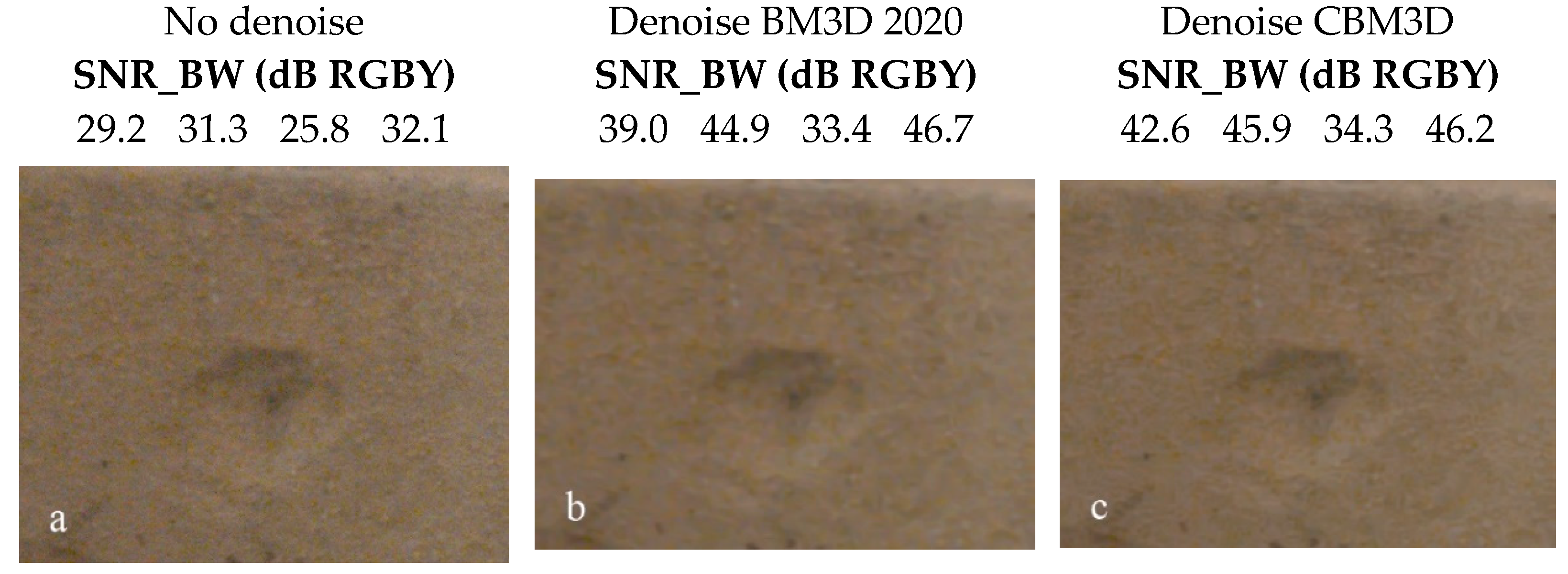
6.4.1. Color Fidelity and Denoise Effects

The evaluation of color accuracy, based on the CCP target and the rendered color space sRGB, is computed according to the following parameters: mean and max color difference relative to the mean ideal chroma in the CIEDE2000 color metric on the CIEXYZ chromaticity diagram; mean of absolute luminance; exposure error in f-stops measured by pixel levels of patches B4-E4, using gamma values measured rather than the standard value for the color space (i.e., in the case of sRGB 2.2). As reference values for the ΔE*00 we used the analysis of [107] that demonstrated how the perceptible and acceptable color differences in complex images presented on a CRT monitor vary approximately between 2.2 and 4.5, depending on the lighting conditions and the environment in which the image is observed. The Δ L 00 mean of absolute luminance less than 1 is required; the exposure error in f-stops best results are obtained if it is less than 0.25 f-stops. We compared the iPhone X values with those captured with the Nikon D5200 SLR camera, an excellent reference as it was the main camera on which the SHAFT was developed.
For the denoise, we evaluated:
  • the efficiency of CBM3D-new compared to the standard implementation of the BM3D;
  • SNR (signal-to-noise ratio) expressed in decibel for the patch 19–24 of the CCP target for R, G, B and L (luminance):
S N R ( d B ) = 20 l o g 10 ( S i N i ) ,
where Si is the signal (mean pixel level) of patch i and Ni is the noise (standard deviation of the pixel level, with slow variations removed) of patch i. In practice we measured the SNRBW, an average SNR based on White-Black patches (patch 19–patch 24; density difference = 1.45:
S N R B W = 20 l o g 10 ( S W H I T E S B L A C K N m i d ) ,
where Nmid is the noise in the patch 22 (middle gray; closest to nominal chart density = 0.7).
All calculations were made using the Imatest Master (Imatest LLC, Boulder, CO, USA) software version 2020, which lets users evaluate tone reproduction, color fidelity, noise and exposure error [108].

6.4.2. Calibration Effects

We evaluated the effects of the camera calibration on all the four selected objects to check the improvement achieved using this procedure against the self-calibration from EXIF data in the SFM process.

6.4.3. Photogrammetric Pipeline Efficiency

The performances of the photogrammetric pipeline were evaluated by a statistical analysis that considered the following parameters:
  • the number of oriented images;
  • Bundle Adjustment (BA) (re-projection error);
  • number of points collected in the dense point cloud. The dense matching procedure was applied using n-frames SURE starting from the camera orientation results achieved in COLMAP. The absolute number of points extracted and the point density distribution (the Local Density Computation–LDC) for the different dense clouds were estimated using the software CloudCompare [109]. The LDC tool counts, for each 3D point of the cloud, the number of neighbors N (inside a sphere of a radius R, fixed at 2 cm);
  • the comparison of the dense point cloud to the ground truth of the object. The four photogrammetric models were compared with the TLS and the SLR camera models using CloudCompare. The comparison is preceded by an alignment and registration phase to correctly align reconstruction and reference laser scanned model. The alignment is guaranteed by a two-step process: a first phase of coarse alignment, performed manually by specifying pairs of corresponding points that are aligned using the Horn technique [110] and a second phase of fine registration, did using the Iterative Closest Point (ICP) algorithm [111,112].

7. Results

To evaluate the accuracy and the performance of the proposed image-based modeling method, three functionalities were tested in small/medium museum scenarios:
  • color fidelity and denoise effects;
  • calibration effects;
  • photogrammetry pipeline.
A. Color fidelity and denoise effects
As far as color fidelity is concerned, the tests showed absolute comparability between the results obtained with the iPhone X smartphone and the Nikon D5200 camera. The ΔE*00 mean error values of SLR and smartphone camera are very close that is, the color differences are indistinguishable (Table 6), while the ΔL* values are practically identical. In general, we observe how controlled light conditions lead to relevant benefits in the ΔE*00 Max values (more than 1 ΔE*00) mainly in the case of the iPhone X camera. In Figure 21 is reported the denoise reduction efficiency of our variant CBM3D-new against the standard implementation of the BM3D and the image not denoised in terms of S N R B W for a noisy image. In Table 7 are reported mean values of each dataset showing systematic advantages in the ΔE*00, Exposure error and SNR (signal-to-noise ratio) values.
In Figure 22 is the comparison of the final 3D model of the Heracles before and after the CC.
B. Calibration results and effects
Calibration results are presented in Table 8. In addition to the elementary interior orientation parameters (Cx, Cy, f), two radial lens distortion parameters were extracted (k1, k2), as well as the first two decentering lens distortion parameters (P1, P2). Every parameter was checked for statistical determinability and those below 99% were removed. Results show little differences between the techniques. Calibration effects on number of oriented images, BA re-projection error and number of points in the dense point cloud are in Table 9, which demonstrates the efficiency of the SfM reconstruction process, achieving the same results than those obtained using the geometric camera calibration process.
C. Performance evaluation of Photogrammetry pipeline
In Table 10 are reported the results of the evaluation of the photogrammetric performance for both the Nikon D5200 with an 18-mm nominal focal length and iPhone X with a 4 mm lens length. The results concerning the number of oriented images and mean reprojection error of the Bundle Adjustment of the two cameras are comparable. On the contrary, the number of points collected in the dense point cloud are different but congruent with the number of pixels in the image set: those acquired by Nikon D5200 doubled those in the iPhone X camera image set. The LDC computation (represented as color-coded maps and histograms in Table 11) shows, for the different objects acquired using iPhone X, the related amount of 3D points and the type of neighboring distribution. The histograms show, for the Porcupinefish, a polarized distribution due to the surface characterized by the quills. On the contrary, in the case of the Globe, a very wide range of distribution was observed. This was caused by the marked difference in surface treatment between the globe and the pedestal In the other two cases, we observed a Gaussian-like distribution, albeit more shifted towards the low values for the statue of Hercules, due to the shooting environment that affected the acquiring data sets. The evaluation of the dense points cloud reconstructed of the objects acquired takes place in terms of the distance between the reconstructed points and the geometry of the ground truth.
The accuracy evaluation of the dense matching results is done using, as ground truth, the TLS Faro Focus3D for Hercules statue and the NextEngine for the Porcupinefish, the Globe and the Marsili bust. The average image GSD (Ground Sample Distance) in both models (reference and data comparison) is ≈1 mm, therefore we had not to re-sampling any dense point clouds to have a reference comparable to the dense matching results. Figure 23 and Table 12 summarize the results from iPhone X vs. Ground truth models comparison showing, in accordance with the objectives set, an excellent reliability in terms of morphology and consistency of the method adopted.
Concerning morphological results coming from deviation analysis on a difficult subject such as the Porcupinefish, they shown the potentials of smartphone cameras on translucent, tiny elements, as well as when we match with a wide range of materials characterized by different kinds and values of light reflection (diffuse vs. specular, that is, Marsili bust), porosity, transparency and so forth.
Figure 24 summarizes the results of the applied geometric process—from quad-dominant to textured model—showing accurate visual representations of the acquired objects (here the Marsili’s bust).

8. Discussion

Over the last decade, smartphone camera technologies significantly improved, achieving performance very similar to prosumer SLR cameras in terms of image resolution, sharpness and color reproduction accuracy. Due to this reason, as also witnessed by [37,38,39], smartphones have attracted the attention of scholars to be used as tools for generating high-quality 3D models in the field of CH. Most of the research, up to now, have been mainly focused on radiometric precision [40,41,42]. Through this work we verified how smartphone cameras can reach high quality results within a specific and adequate photogrammetric pipeline, in the reproduction of colors, by obtaining ΔE*00 mean error values and for what concerns ΔL* values, which are practically identical to those of the SLR cameras (that means almost indistinguishable color differences). This result confirms that we are at the beginning of a new era in the field of museum management. The level of visual quality of the 3D models produced is suitable both for a general audience (e.g., museum visitors), that will experience the model through RTR Systems (Figure 25), that requires low-poly models (‘derived’ from high-poly); and for field experts (e.g., scholars) that will consult the high-poly version (‘Master Model’).
However, the increasingly pervasive use of in-camera software to automate different types of frame capture and the image processing to achieve ‘pleasant’ quality of the results are both elements to be carefully considered. These ‘black-box’ image manipulations, which are automatically carried out and not transparent to the final user due to copyrighted algorithms from major software houses, could entail problems in the possibility of tracing back the raw data, a main requirement to get accurate 3D models from the photogrammetric pipeline and high-quality RTR visualization. Great part of our study was aimed at automatically restore images original features through a sort of ‘reverse engineering’ process. The developed workflow, though largely automated to be easy to use, is quite flexible and it features many stages, such as setting parameters from the image metadata, denoising and CC the entire dataset to improve the automated 3D reconstruction procedure. Since in-camera image processing increases every year, it is very probable that the research must turn its attention towards the development of algorithms able to trace the original characteristics (RAW data) of the acquired frame to achieve more and more accurate 3D models.
Furthermore, results demonstrated that our selected set of devices it can capture accurate 3D models, besides their small size and their general-purpose or low-cost features. This is, in our opinion, a major achievement in the field of medium-small museums, where complex equipment is generally out of place. This could open new research aiming to optimize this type of minimal and general-purpose infrastructures.

9. Conclusions

This work analyzes and proposes a workflow to foster the increasingly widespread use of digital technologies in the field of small-medium museum management, capable of producing, among the other benefits, 3D representations of museum objects following a precise workflow, from the acquisition phase to the final visualization in RTR.
We also presented a set of instruments accurately selected to meet the everyday needs of museums activities (cataloguing, conservation, analysis, dissemination).
Our workflow and tools were then assessed on four case studies representing some of the most common problems that arise acquiring museum collections.
Results demonstrate that devices and workflow allow to get high-quality 3D models that can be used for the management and enhancement of CH, together with monitoring the state of preservation, production of audio-visual and interactive systems for scientific dissemination tools, among the other possible uses. The related new way of working potentially appears, then, as a major change in the activities of conservators, fine art specialists, archaeologists, historians and scholars.
However, the achieved results highlighted that further progress are possible and desirable on some unsolved issues. One of these concerns the extension of the case studies to be able to identify and address additional problems of devices and workflow; another is the complete automation of the pipeline, through procedural algorithms and Deep Learning applications for Derivative models construction.

Author Contributions

All authors equally contributed to the procedure development, data processing and paper preparation. All authors have read and agreed to the published version of the manuscript.

Funding

This research received no external funding.

Data Availability Statement

Not applicable.

Acknowledgments

Authors would like to thank the Sistema Museale di Ateneo (SMA) of University of Bologna, which gave us access to the artifacts of its collections, in particular the Director Roberto Balzani, the Technical Coordinator Annalisa Managlia and all the management staff. The work was accomplished with the technical support of Relio (https://www.relio.it/).

Conflicts of Interest

The authors declare no conflict of interest.

References

  1. Negri, M.; Marini, G. Le 100 Parole dei Musei; Marsilio: Venezia, Italy, 2020. [Google Scholar]
  2. Europeana DSI 2—Access to Digital Resources of European Heritage—Deliverable D4.4. Report on ENUMERATE Core Survey 4. Available online: https://pro.europeana.eu/files/Europeana_Professional/Projects/Project_list/Europeana_DSI-2/Deliverables/ (accessed on 17 November 2020).
  3. Europeana Pro. Available online: https://pro.europeana.eu/page/digital-collections (accessed on 17 November 2020).
  4. Grussenmeyer, P.; Al Khalil, O. A Comparison of Photogrammetry Software Packages for the Documentation of Buildings. In Proceedings of the International Federation of Surveyors, Saint Julian’s, Malta, 18–21 September 2000. [Google Scholar]
  5. Nocerino, E.; Stathopoulou, E.K.; Rigon, S.; Remondino, F. Surface Reconstruction Assessment in Photogrammetric Applications. Sensors 2020, 20, 5863. [Google Scholar] [CrossRef] [PubMed]
  6. Deseilligny, M.P.; De Luca, L.; Remondino, F. Automated image-based procedures for accurate artefacts 3D modeling and orthoimage generation. J. Geoinformatics FCE CTU 2011, 6. [Google Scholar] [CrossRef]
  7. Petrelli, D. Making virtual reconstructions part of the visit: An exploratory study. Digit. Appl. Archaeol. Cult. Herit. 2019, 15, e00123. [Google Scholar] [CrossRef]
  8. Pierdicca, R.; Frontoni, E.; Zingaretti, P.; Sturari, M.; Clini, P.; Quattrini, R. Advanced Interaction with Paintings by Augmented Reality and High-Resolution Visualization: A Real Case Exhibition. In Augmented and Virtual Reality. AVR 2015; Lecture Notes in Computer Science; Springer: Cham, Germany, 2015; Volume 9254. [Google Scholar]
  9. Berthelot, M.; Nony, N.; Gugi, L.; Bishop, A.; De Luca, L. The Avignon Bridge: A 3D reconstruction project integrating archaeological, historical and geomorphological issues. Int. Arch. Photogramm. Remote Sens. Spat. Inf. Sci. 2015, 40, 223–227. [Google Scholar] [CrossRef] [Green Version]
  10. Fassi, F.; Mandelli, A.; Teruggi, S.; Rechichi, F.; Fiorillo, F.; Achille, C. VR for Cultural Heritage. Augmented Reality, Virtual Reality, and Computer Graphics. AVR 2016; Lecture Notes in Computer Science; Springer: Cham, Germany, 2016; Volume 9769. [Google Scholar]
  11. Pescarin, S.; D’Annibale, E.; Fanini, B.; Ferdani, D. Prototyping on site Virtual Museums: The case study of the co-design approach to the Palatine hill in Rome (Barberini Vineyard) exhibition. In Proceedings of the 3rd Digital Heritage International Congress (DigitalHERITAGE) Held Jointly with 24th International Conference on Virtual Systems & Multimedia (VSMM 2018), San Francisco, CA, USA, 26–30 October 2018; pp. 1–8. [Google Scholar]
  12. Agus, M.; Marton, F.; Bettio, F.; Hadwiger, M.; Gobbetti, E. Data-Driven Analysis of Virtual 3D Exploration of a Large Sculpture Collection in Real-World Museum Exhibitions. J. Comput. Cult. Herit. 2018, 11, 1–20. [Google Scholar] [CrossRef]
  13. Available online: https://www.cultlab3d.de/ (accessed on 21 November 2020).
  14. Available online: http://witikon.eu/ (accessed on 21 November 2020).
  15. Menna, F.; Nocerino, E.; Morabito, D.; Farella, E.M.; Perini, M.; Remondino, F. An open source low-cost automatic system for image-based 3D digitization. Int. Arch. Photogramm. Remote Sens. Spat. Inf. Sci. 2017, 42, 155–162. [Google Scholar] [CrossRef] [Green Version]
  16. Potenziani, M.; Callieri, M.; Dellepiane, M.; Corsini, M.; Ponchio, F.; Scopigno, R. 3DHOP: 3D Heritage Online Presenter. Comput. Graph. 2015, 52, 129–141. [Google Scholar] [CrossRef]
  17. Available online: https://sketchfab.com/ (accessed on 13 June 2020).
  18. Available online: https://sketchfab.com/britishmuseum (accessed on 21 November 2020).
  19. Gaiani, M.; Apollonio, F.I.; Fantini, F. Evaluating smartphones color fidelity and metric accuracy for the 3D documentation of small artefacts. Int. Arch. Photogramm. Remote Sens. Spat. Inf. Sci. 2019, 42, 539–547. [Google Scholar] [CrossRef] [Green Version]
  20. Apollonio, F.I.; Foschi, R.; Gaiani, M.; Garagnani, S. How to analyze, preserve, and communicate Leonardo’s drawing? A solution to visualize in RTR fine art graphics established from “the best sense”. J. Comput. Cult. Herit. 2020. [Google Scholar]
  21. Akca, D.; Gruen, A. Comparative geometric and radiometric evaluation of mobile phone and still video cameras. Photogramm. Rec. 2009, 24, 217–245. [Google Scholar] [CrossRef]
  22. Tanskanen, P.; Kolev, K.; Meier, L.; Camposeco, F.; Saurer, O.; Pollefeys, M. Live metric 3D reconstruction on mobile phones. In Proceedings of the IEEE International Conference on Computer Vision, Sydney, NSW, Australia, 1–8 December 2013; pp. 65–72. [Google Scholar]
  23. Kos, A.; Tomažič, S.; Umek, A. Evaluation of Smartphone Inertial Sensor Performance for Cross-Platform Mobile Applications. Sensors 2016, 16, 477. [Google Scholar] [CrossRef] [PubMed] [Green Version]
  24. Smartphones vs Cameras: Closing the Gap on Image Quality, Posted on 19 March 2020 by David Cardinal 2020. Available online: https://www.dxomark.com/smartphones-vs-cameras-closing-the-gap-on-image-quality/ (accessed on 21 November 2020).
  25. Nocerino, E.; Lago, F.; Morabito, D.; Remondino, F.; Porzi, L.; Poiesi, F.; Rota Bulo, S.; Chippendale, P.; Locher, A.; Havlena, M.; et al. A smartphone-based 3D pipeline for the creative industry—The REPLICATE EU Project. Int. Arch. Photogramm. Remote Sens. Spat. Inf. Sci. 2017, 42, 535–541. [Google Scholar] [CrossRef] [Green Version]
  26. Poiesi, F.; Locher, A.; Chippendale, P.; Nocerino, E.; Remondino, F.; Van Gool, L. Cloud-based collaborative 3D reconstruction using smartphones. In Proceedings of the 14th European Conference on Visual Media Production (CVMP 2017), London, UK, 11–13 December 2017; ACM: New York, NY, USA, 2017; pp. 1–9. [Google Scholar]
  27. Pintore, G.; Garro, V.; Ganovelli, F.; Agus, M.; Gobbetti, E. Omnidirectional image capture on mobile devices for fast automatic generation of 2.5D indoor maps. In Proceedings of the IEEE Winter Conference on Applications of Computer Vision (WACV), Lake Placid, NY, USA, 7–10 March 2016; pp. 1–9. [Google Scholar]
  28. Ondruska, P.; Kohli, P.; Izad, S. MobileFusion: Real-time Volumetric Surface Reconstruction and Dense Tracking on Mobile Phones. IEEE Trans. Vis. Comput. Graph. 2015, 21, 1251–1258. [Google Scholar] [CrossRef] [PubMed]
  29. Apollonio, F.I.; Gaiani, M.; Baldissini, S. Color definition of open-air Architectural heritage and Archaeology artworks with the aim of conservation. Digit. Appl. Archaeol. Cult. Herit. 2017, 7, 10–31. [Google Scholar]
  30. Gaiani, M.; Remondino, F.; Apollonio, F.I.; Ballabeni, A. An Advanced Pre-Processing Pipeline to Improve Automated Photogrammetric Reconstructions of Architectural Scenes. Remote Sens. 2016, 8, 178. [Google Scholar] [CrossRef] [Green Version]
  31. Gaiani, M.; Apollonio, F.I.; Bacci, G.; Ballabeni, A.; Bozzola, M.; Foschi, R.; Garagnani, S.; Palermo, R. Seeing inside drawings: A system for analysing, conserving, understanding and communicating Leonardo’s drawings. In Leonardo in Vinci. At the Origins of the Genius; Giunti Editore: Milano, Italy, 2019; pp. 207–240. [Google Scholar]
  32. Ullman, S. The interpretation of structure from motion. Proc. R. Soc. Lond. 1979, 203, 405–426. [Google Scholar]
  33. Hartley, R.; Zisserman, A. Multiple View Geometry in Computer Vision; Cambridge University Press: New York, NY, USA, 2003. [Google Scholar]
  34. Hartmann, W.; Havlena, M.; Schindler, K. Recent developments in large-scale tie-point matching. Int. Arch. Photogramm. Remote Sens. Spat. Inf. Sci. 2016, 115, 47–62. [Google Scholar] [CrossRef]
  35. Schonberger, J.L.; Frahm, J.-M. Structure-from-motion revisited. In Proceedings of the IEEE Conference on Computer Vision and Pattern Recognition, Las Vegas, NV, USA, 27–30 June 2016; pp. 4104–4113. [Google Scholar]
  36. Remondino, F.; Spera, M.G.; Nocerino, E.; Menna, F.; Nex, F. State of the art in high density image matching. Photogramm. Rec. 2014, 146, 144–166. [Google Scholar] [CrossRef] [Green Version]
  37. Gonizzi-Barsanti, S.; Remondino, F.; Jiménez Fernández-Palacios, B.; Visintini, D. Critical factors and guidelines for 3D surveying and modelling in Cultural Heritage. Int. J. Herit. Digit. Era 2015, 3, 142–158. [Google Scholar]
  38. Toschi, I.; Capra, A.; De Luca, L.; Beraldin, J.-A.; Cournoyer, L. On the evaluation of photogrammetric methods for dense 3D surface reconstruction in a metrological context. In ISPRS Annals of the Photogrammetry, Remote Sensing and Spatial Information Sciences, Proceedings of the ISPRS Technical Commission V Symposium, Riva del Garda, Italy, 23–25 June 2014; ISPRS: Hannover, Germany, 2014; Volume 2, pp. 371–378. [Google Scholar]
  39. Remondino, F.; Gaiani, M.; Apollonio, F.I.; Ballabeni, A.; Ballabeni, M.; Morabito, D. 3D Documentation of 40 Km of Historical Porticoes—The Challenge. Int. Arch. Photogramm. Remote Sens. Spat. Inf. Sci. 2016, 41, 711–718. [Google Scholar] [CrossRef]
  40. Apollonio, F.I.; Gaiani, M.; Basilissi, W.; Rivaroli, L. Photogrammetry driven tools to support the restoration of open-air bronze surfaces of sculptures: An integrated solution starting from the experience of the Neptune Fountain in Bologna. Int. Arch. Photogramm. Remote Sens. Spat. Inf. Sci. 2017, 42, 47–54. [Google Scholar] [CrossRef] [Green Version]
  41. Apollonio, F.I.; Ballabeni, M.; Bertacchi, S.; Fallavollita, F.; Foschi, R.; Gaiani, M. From documentation images to restauration support tools: A path following the Neptune Fountain in Bologna design process. Int. Arch. Photogramm. Remote Sens. Spat. Inf. Sci. 2017, 42, 329–336. [Google Scholar] [CrossRef] [Green Version]
  42. Remondino, F.; Nocerino, E.; Toschi, I.; Menna, F. A critical review of automated photogrammetric processing of large datasets. Int. Arch. Photogramm. Remote Sens. Spat. Inf. Sci. 2017, 42, 591–599. [Google Scholar] [CrossRef] [Green Version]
  43. Barsanti, S.G.; Guidi, G.; De Luca, L. Segmentation of 3D Models for Cultural Heritage Structural Analysis–Some Critical Issues. ISPRS Ann. Photogramm. Remote Sens. Spat. Inf. Sci. 2017, 4, 115. [Google Scholar] [CrossRef] [Green Version]
  44. Grilli, E.; Remondino, F. Classification of 3D Digital Heritage. Remote Sens. 2019, 11, 847. [Google Scholar] [CrossRef] [Green Version]
  45. Oses, N.; Dornaika, F.; Moujahid, A. Image-based delineation and classification of built heritage masonry. Remote Sens. 2014, 6, 1863–1889. [Google Scholar] [CrossRef] [Green Version]
  46. Rushmeier, H.; Bernardini, F.; Mittleman, J.; Taubin, G. Acquiring Input for Rendering at Appropriate Levels of Detail: Digitizing a Pietà. In Rendering Techniques ’98. EGSR 1998; Eurographics; Springer: Vienna, Austria, 1998. [Google Scholar]
  47. Apollonio, F.I.; Gaiani, M.; Benedetti, B. 3D reality-based artefact models for the management of archaeological sites using 3D GIS: A framework starting from the case study of the Pompeii Archaeological area. J. Archaeol. Sci. 2012, 39, 1271–1287. [Google Scholar] [CrossRef]
  48. Nicodemus, F.E. Directional reflectance and emissivity of an opaque surface. Appl. Opt. 1965, 4, 767–775. [Google Scholar] [CrossRef]
  49. Guarnera, D.; Guarnera, G.C.; Ghosh, A.; Denk, C.; Glencross, M. BRDF Representation and Acquisition. Comput. Graph. Forum 2016, 35, 625–650. [Google Scholar] [CrossRef] [Green Version]
  50. Westin, S.H.; Arvo, J.; Torrance, K.E. Predicting reflectance functions from complex surfaces. In Proceedings of the SIGGRAPH 92; ACM: New York, NY, USA, 1992; pp. 255–264. [Google Scholar]
  51. Torrance, K.E.; Sparrow, E.M. Theory for off-specular reflection from roughened surfaces. J. Opt. Soc. Am. 1967, 57, 1105–1114. [Google Scholar] [CrossRef]
  52. Burley, B. Extending Disney’s Physically Based BRDF with Integrated Subsurface Scattering. In SIGGRAPH’15 Courses; ACM: New York, NY, USA, 2015; Article 22. [Google Scholar]
  53. Goral, C.M.; Torrance, K.E.; Greenberg, D.P.; Battaile, B. Modeling the Interaction of Light between Diffuse Surfaces. In Proceedings of the SIGGRAPH 84; ACM: New York, NY, USA, 1984; pp. 213–222. [Google Scholar]
  54. Stamatopoulos, C.; Fraser, C.; Cronk, S. Accuracy aspects of utilizing RAW imagery in photogrammetric measurement. ISPRS Int. Arch. Photogramm. Remote Sens. Spat. Inf. Sci. 2012, 39, 387–392. [Google Scholar] [CrossRef] [Green Version]
  55. IEEE. IEEE Standard for Camera Phone Image Quality (CPIQ); IEEE P1858; IEEE: New York, NY, USA, 2017. [Google Scholar]
  56. ISO. Graphic Technology and Photography—Color Characterisation of Digital Still Cameras (DSCs); ISO 17321-1; Standardization, I.O.F.; ISO: Geneva, Switzerland, 2012. [Google Scholar]
  57. Wandell, B.A.; Farrell, J.E. Water into wine: Converting scanner RGB to tristimulus XYZ. Device-Indep. Color Imaging Imaging Syst. Integr. 1993, 1909, 92–100. [Google Scholar]
  58. McCamy, C.S.; Marcus, H.; Davidson, J. A color-rendition chart. J. Appl. Photogr. Eng. 1976, 2, 95–99. [Google Scholar]
  59. Botsch, M.; Kobbelt, L.; Pauly, M.; Alliez, P.; Levy, B. Polygon Mesh Processing; A K Peters: Natick, MA, USA; CRC Press: Boca Raton, FL, USA, 2010. [Google Scholar]
  60. Alliez, P.; Ucelli, G.; Gotsman, C.; Attene, M. Recent Advances in Remeshing of Surfaces. In Shape Analysis and Structuring; De Floriani, L., Spagnuolo, M., Eds.; Springer: Berlin/Heidelberg, Germany, 2008. [Google Scholar]
  61. Alliez, P.; Cohen-Steiner, D.; Devillers, O.; Levy, B.; Desbrun, M. Anisotropic polygonal remeshing. ACM Trans. Graph. 2003, 22, 485–493. [Google Scholar] [CrossRef]
  62. Bommes, D.; Lévy, B.; Pietroni, N.; Puppo, E.; Silva, C.; Tarini, M.; Zorin, D. Quad-Mesh Generation and Processing: A Survey. Comput. Graph. Forum 2013, 32, 51–76. [Google Scholar] [CrossRef]
  63. Guidi, G.; Angheleddu, D. Displacement Mapping as a Metric Tool for Optimizing Mesh Models Originated by 3D Digitization. ACM J. Comput. Cult. Herit. 2016, 9, 1–23. [Google Scholar] [CrossRef] [Green Version]
  64. Schertler, N.; Tarini, M.; Jakob, W.; Kazhdan, M.; Gumhold, S.; Panozzo, D. Field-Aligned Online Surface Reconstruction. ACM Trans. Graph. 2017, 36, 1–13. [Google Scholar] [CrossRef] [Green Version]
  65. De Rose, T.; Kass, M.; Truong, T. Subdivision surfaces in character animation. In Proceedings of the SIGGRAPH 98; ACM: New York, NY, USA, 1998; pp. 85–94. [Google Scholar]
  66. Akenine-Möller, T.; Haines, E.; Hoffman, N. Real-Time Rendering, 4th ed.; Taylor & Francis: Abingdon, UK; CRC Press: Boca Raton, FL, USA, 2018. [Google Scholar]
  67. Blinn, J.F. Simulation of Wrinkled Surfaces. Comput. Graph. 1978, 12, 286–292. [Google Scholar] [CrossRef]
  68. Cohen, J.; Olano, M.; Manocha, D. Appearance-Preserving Simplification. In Proceedings of the SIGGRAPH 98; ACM: New York, NY, USA, 1998; pp. 115–122. [Google Scholar]
  69. Cignoni, P.; Montani, C.; Scopigno, R.; Rocchini, C. A general method for preserving attribute values on simplified meshes. In Proceedings of the Conference on Visualization ‘98 (VIS ‘98), Research Triangle Park, NC, USA, 18–23 October 1998; pp. 59–66. [Google Scholar]
  70. Woodham, R.J. Photometric method for determining surface orientation from multiple images. Opt. Eng. 1980, 19, 139–144. [Google Scholar] [CrossRef]
  71. Relio2. Available online: www.relio.it (accessed on 17 November 2020).
  72. Collins, T.; Woolley, S.I.; Gehlken, E.; Ch’ng, E. Automated Low-Cost Photogrammetric Acquisition of 3D Models from Small Form-Factor Artefacts. Electronics 2019, 8, 1441. [Google Scholar] [CrossRef] [Green Version]
  73. Kraus, K. Photogrammetry. Advanced Methods and Applications; Dummler: Bonn, Germany, 1997; Volume 2. [Google Scholar]
  74. Gaiani, M.; Apollonio, F.I.; Ballabeni, A.; Remondino, F. Securing Color Fidelity in 3D Architectural Heritage Scenarios. Sensors 2017, 17, 2437. [Google Scholar] [CrossRef] [PubMed] [Green Version]
  75. Morel, J.-M.; Yu, G. ASIFT: A new framework for fully affine invariant comparison. SIAM J. Imaging Sci. 2009, 2, 438–469. [Google Scholar] [CrossRef]
  76. Gaiani, M. I Portici di Bologna Architettura, Modelli 3D e Ricerche Tecnologiche; Bononia University Press: Bologna, Italy, 2015. [Google Scholar]
  77. Fischler, M.A.; Bolles, R.C. Random Sample Consensus: A Paradigm for Model Fitting with Applications to Image Analysis and Automated Cartography. Commun. ACM 1981, 24, 381–395. [Google Scholar] [CrossRef]
  78. Triggs, B.; McLauchlan, P.F.; Hartley, R.I.; Fitzgibbon, A.W. Bundle adjustment—A modern synthesis. In International Workshop on Vision Algorithms; Springer: Berlin/Heidelberg, Germany, 1999; pp. 298–372. [Google Scholar]
  79. Schönberger, J.L.; Zheng, E.; Pollefeys, M.; Frahm, J.M. Pixelwise View Selection for Unstructured Multi-View Stereo. In Proceedings of the European Conference on Computer Vision (ECCV), Amsterdam, The Netherlands, 8–16 October 2016. [Google Scholar]
  80. Wenzel, K.; Rothermel, M.; Haala, N.; Fritsch, D. SURE–The Ifp Software for Dense Image Matching; Wichmann: Berlin/Offenbach, Germany; VDE Verlag: Berlin, Germany, 2013. [Google Scholar]
  81. Hirschmüller, H. Stereo processing by semiglobal matching and mutual information. IEEE Trans. Pattern Anal. Mach. Intell. 2007, 30, 328–341. [Google Scholar]
  82. Jakob, W.; Tarini, M.; Panozzo, D.; Sorkine-Hornung, O. Instant field-aligned meshes. ACM Trans. Graph. 2015, 34, 6. [Google Scholar] [CrossRef]
  83. García-León, J.; Sánchez-Allegue, P.; Peña-Velasco, C.; Cipriani, L.; Fantini, F. Interactive dissemination of the 3D model of a baroque altarpiece: A pipeline from digital survey to game engines. SCIRES-IT Sci. Res. Inf. Technol. 2018, 8, 59–76. [Google Scholar]
  84. Ballabeni, A.; Apollonio, F.; Gaiani, M.; Remondino, F. Advances in image pre-processing to improve automated 3D reconstruction. ISPRS Int. Arch. Photogramm. Remote Sens. Spat. Inf. Sci. 2015, 40, 315–323. [Google Scholar] [CrossRef] [Green Version]
  85. Karaimer, H.C.; Brown, M.S. A Software Platform for Manipulating the Camera Imaging Pipeline. In Computer Vision—ECCV 2016; Lecture Notes in Computer Science; Leibe, B., Matas, J., Sebe, N., Welling, M., Eds.; Springer: Cham, Germany, 2016; Volume 9905, pp. 429–444. [Google Scholar]
  86. Dabov, K.; Foi, A.; Katkovnik, V.; Egiazarian, K. Image denoising by sparse 3-D transform-domain collaborative filtering. IEEE Trans. Image Process. 2007, 16, 2080–2095. [Google Scholar] [CrossRef]
  87. Mäkinen, Y.; Azzari, L.; Foi, A. Collaborative Filtering of Correlated Noise: Exact Transform-Domain Variance for Improved Shrinkage and Patch Matching. IEEE Trans. Image Process. 2020, 29, 8339–8354. [Google Scholar] [CrossRef]
  88. Plötz, T.; Roth, S. Benchmarking Denoising Algorithms with Real Photographs. In Proceedings of the IEEE Conference on Computer Vision and Pattern Recognition (CVPR), Honolulu, HI, USA, 21–26 July 2017; pp. 2750–2759. [Google Scholar]
  89. Pascale, D. RGB Coordinates of the Macbeth ColourChecker; The BabelColour Company: Montreal, QC, Canada, 2006; pp. 1–16. [Google Scholar]
  90. Available online: https://www.xrite.com/service-support/new_color_specifications_for_colorchecker_sg_and_classic_charts (accessed on 21 November 2020).
  91. Wyszecki, G.; Stiles, W.S. Color Science—Concepts and Methods, Quantitative Data and Formulae; Wiley: Danvers, MA, USA, 2000. [Google Scholar]
  92. Gaiani, M.; Ballabeni, A. SHAFT (SAT & HUE Adaptive Fine Tuning), a new automated solution for target-based color correction. Color Colorimetry Multidiscip. Contrib. 2018, 14, 69–80. [Google Scholar]
  93. Available online: https://github.com/Beep6581/RawTherapee (accessed on 21 November 2020).
  94. Kim, E.-S.; Lee, S.-H.; Jang, S.-W.; Sohng, K.-I. Adaptive colorimetric characterization of camera for the variation of white balance. IEICE Trans. Electron. 2005, 88, 2086–2089. [Google Scholar] [CrossRef] [Green Version]
  95. Sharma, G.; Wu, W.; Dalal, E.N. The CIEDE2000 Color-Difference Formula: Implementation Notes, Supplementary Test Data, and Mathematical Observations. Color Res. Appl. 2005, 30, 21–30. [Google Scholar] [CrossRef]
  96. ISO. Colorimetry—Part 6: CIEDE2000 Color-Difference Formula; ISO/CIE 11664-6; ISO: Geneva, Switzerland, 2014. [Google Scholar]
  97. Melgosa, M.; Alman, D.H.; Grosman, M.; Gómez-Robledo, L.; Trémeau, A.; Cui, G.; García, P.A.; Vázquez, D.; Li, C.; Luo, M.R. Practical demonstration of the CIEDE2000 corrections to CIELAB using a small set of sample pairs. Color Res. Appl. 2013, 38, 429–436. [Google Scholar] [CrossRef]
  98. Mokrzycki, W.S.; Tatol, M. Color difference Delta E—A survey. Mach. Graph. Vis. 2012, 20, 383–411. [Google Scholar]
  99. Stokes, M.; Anderson, M.; Chandrasekar, S.; Motta, R. A Standard Default Color Space for the Internet-sRGB. 1996. Available online: http://www.w3.org/Graphics/Color/sRGB.html (accessed on 17 November 2020).
  100. Botsch, M.; Kobbelt, L. A Remeshing Approach to Multiresolution Modeling. In Proceedings of the Eurographics/ACM SIGGRAPH Symposium on Geometry Processing, SGP ‘04, Nice, France, 8–10 July 2004; ACM: New York, NY, USA, 2004; pp. 185–192. [Google Scholar]
  101. Dunyach, M.; Vanderhaeghe, D.; Barthe, L.; Botsch, M. Adaptive Remeshing for Real-Time Mesh Deformation. In Proceedings of the Eurographics 2013, Girona, Spain, 6–10 May 2013; The Eurographics Association: Geneve, Switzerland, 2013; pp. 29–32. [Google Scholar]
  102. Mikkelsen, M. Simulation of Wrinkled Surfaces Revisited. Master’s Thesis, University of Copenhagen, Copenhagen, Denmark, 26 March 2008. [Google Scholar]
  103. Cipriani, L.; Fantini, F.; Bertacchi, S. 3D models mapping optimization through an integrated parameterization approach: Cases studies from Ravenna. ISPRS Int. Arch. Photogramm. Remote Sens. Spat. Inf. Sci. 2014, 45, 173–180. [Google Scholar] [CrossRef] [Green Version]
  104. Brown, D.C. Close-range camera calibration. Photogramm. Eng. 1971, 37, 855–866. [Google Scholar]
  105. Fryer, J.G. Camera calibration. In Close Range Photogrammetry and Machine Vision; Atkinson, K.B., Ed.; Chapter 6; Whittles Publishing: Dunbeath, UK, 2001; pp. 156–179. [Google Scholar]
  106. Remondino, F.; Fraser, C.S. Digital camera calibration methods: Considerations and comparisons. ISPRS Int. Arch. Photogramm. Remote Sens. Spat. Inf. Sci. 2006, 36, 266–272. [Google Scholar]
  107. Song, T.; Luo, M.R. Testing color-difference formulae on complex images using a CRT monitor. In Proceedings of the IS & T and SID Eighth Color Imaging Conference, Scottsdale, AZ, USA, 7–10 November 2000; pp. 44–48. [Google Scholar]
  108. Imatest, L. 2020. Available online: https://www.imatest.com/products/imatest-master/ (accessed on 29 January 2021).
  109. Girardeau-Montaut, D. CloudCompare (Version 2.11.2) [GPL Software]. 2020. Available online: http://www.cloudcompare.org/ (accessed on 18 June 2020).
  110. Horn, B.K. Closed-form solution of absolute orientation using unit quaternions. JOSA A 1987, 4, 629–642. [Google Scholar] [CrossRef]
  111. Chen, Y.; Medioni, G. Object modelling by registration of multiple range images. Image Vis. Comput. 1992, 10, 145–155. [Google Scholar] [CrossRef]
  112. Rusinkiewicz, S.; Levoy, M. Efficient variants of the ICP algorithm. In Proceedings of the Third International Conference on 3-D Digital Imaging and Modeling, Quebec City, QC, Canada, 28 May–1 June 2001; pp. 145–152. [Google Scholar]
Figure 1. Results from our workflow.
Remotesensing 13 00486 g001
Figure 2. Main steps of the proposed workflow and final 3D models.
Remotesensing 13 00486 g002
Figure 3. Acquisition set: led light illuminator kit with Relio2 (a); white translucent canvas box (b). In both figures, the rotating support with coded target cubes radially placed along its thickness is visible.
Remotesensing 13 00486 g003
Figure 4. Main issues to ensure an appropriate depth of field using iPhone X.
Remotesensing 13 00486 g004
Figure 5. Calibration set-up scheme (a); 3D test-field formed by 150 RAD coded targets (b).
Remotesensing 13 00486 g005
Figure 6. The proposed workflow.
Remotesensing 13 00486 g006
Figure 7. Extrinsic features: Spatial distribution (SD) (ac); Intrinsic features: Cavity ratio (CR) (df); D/d ratio (right).
Remotesensing 13 00486 g007
Figure 8. The color correction (CC) workflow.
Remotesensing 13 00486 g008
Figure 9. Porcupinefish: 3D model (a); detail (b); simplification process, using automatic isotropic meshes of quadrangular polygons (c) or manual retopology with quads of different size (d).
Remotesensing 13 00486 g009
Figure 10. Porcupinefish: punctual retouches carried out with manual polygonal modelling techniques, on the tops of the spines: optimized triangular mesh (a); automatic quad-dominant remeshing: medium resolution (b); automatic quad-dominant remeshing: low resolution. Topological defects appear on the model: flipped normals and non-manifold faces (c); manual retopology: the result is a highly optimized meshes but it requires skilled users and long time (d).
Remotesensing 13 00486 g010
Figure 11. Marsili bust (detail): the amount of vertex normals (An) to be baked is crucial for the baking process (a); in (b) are shown the corresponding normals of the low-resolution counterparty mesh.
Remotesensing 13 00486 g011
Figure 12. A 2D section of the two overlapping models involved in the baking process with a focus on the quadrangular polygon ABCD (a); a detail of the AB edge of the low-res mesh: every vertex normal of the high-poly is projected onto corresponding texels of the low-poly mesh (b); once baked, normals are applied as a texture map affecting the shading of the low-poly (c); each of the three components defining a vertex normal is encoded in the RGB channels of the bitmap (d).
Remotesensing 13 00486 g012
Figure 13. Example of correct normal texture size determination. For the case of the single island texture in figure where is Fr = 17.3%, bitmap size 256 × 256 and An = 7636; the inequation is 7636 65536 100 17.3 .
Remotesensing 13 00486 g013
Figure 14. A high-poly and three low-poly versions with normal maps applied. Manual retopology guarantees a high visual reliability with small deviations (a); automatic quad-dominant remeshing with small retouches leads to lower resolutions, it increases deviation but still maintains visual reliability (b); automatic intermediate reduction makes the use of normal maps almost unnecessary since the blue base color prevails (R = 128; G = 128; B = 255) (c). A significant deviation between a master model and a low-poly corresponds to a much higher color variety with highly contrasting gradients.
Remotesensing 13 00486 g014
Figure 15. Two approaches to baking: conventional (a) and with a ‘cage’ (or projection cage) (b). The latter can supply baking process with a better flow of the vertex normals.
Remotesensing 13 00486 g015
Figure 16. ‘Waviness’ effect on cylindric and ‘hard-box’ models (a); additional loops of edges do not solve the problem (b); edge hardening on (u,v) island boundaries improves the visual quality (c); increased amount of polygons can solve the problem in combination with edge hardening (d).
Remotesensing 13 00486 g016
Figure 17. The automatic modelling steps (global remeshing and quad-remeshing).
Remotesensing 13 00486 g017
Figure 18. Palazzo Poggi Museum: the Marsili bust in the Military Architecture hall.
Remotesensing 13 00486 g018
Figure 19. General features (D/d ratio; Spatial distribution; Topological complexity, etc.) of micro-/meso-scale objects belonging to museum collections.
Remotesensing 13 00486 g019
Figure 20. Subjects for the testing phase: (a) Hercules; (b) Porcupinefish; (c) Horn d’Arturo Globe; (d) Marsili bust. Each case study is represented with its bounding box and diagonal D (see intrinsic feature). The diagrams at the bottom represent the general features of each object (see Figure 21).
Remotesensing 13 00486 g020
Figure 21. Comparison of our denoise solution (a) with the original BM3D (b) and the image not denoised (c).
Remotesensing 13 00486 g021
Figure 22. Hercules statue 3D model: (a) without CC, (b) with CC.
Remotesensing 13 00486 g022
Figure 23. False-color maps and distribution distance diagrams of dense point cloud comparison: iPhone X vs. Ground truth (a); iPhone X vs. Nikon D5200 (b).
Remotesensing 13 00486 g023
Figure 24. Summary of the pipeline: quad-dominant model (a); parameterization and ‘hardening’ (u,v) boundary islands (b); baked normals from high-poly master model (c); final 3D textured model (d).
Remotesensing 13 00486 g024
Figure 25. 3D geometry displayed into a RTR environment. The textured model can be explored using a custom graphical user interface specifically developed, in which it can be illuminated by different lights or manipulated through touch gestures.
Remotesensing 13 00486 g025
Table 1. Categories of acquisition complexity. Higher scores correspond to a higher complexity level.
INTRINSIC FEATURESEXTRINSIC FEATURES
D/d
D = the Diagonal of the Bounding Box; D = Model Resolution
Cavity Ratio (CR)Surface CharacteristicsSpatial Distribution (SD)Topological Complexity (TC)Boundary
Condition
(BC)
Material ReflectiveMaterial TransmissiveTexture
10 (1)<1 (1)Lambertian (1)Opaque (1)Even distribution (1)3D
X ≃ Y ≃ Z
(1)
0 holes (1)5 sides free (1)
100 (2)1 (2)Dielectric (2)Translucent (2)Odd distribution (2)2D
X ≃ Y >> Z
(2)
1 hole (2)4 sides free (2)
1000 (3)>1 (3)Conductor (3)Transparent (3)Absent (3)1D
X ≃ Y << Z
(3)
2 holes (3)3 sides free (3)
>1000 (N)>>1 (4) n holes (N)2 sides free (4)
Table 2. Features evaluation of collection pieces.
Collection PiecesD/D RatioCavity Ratio (CV)Material ReflectiveMaterial TransmissiveTextureTopological Complexity (TC) (TC)Spatial Distribution (SC) (SD)Boundary
Condition (BC)
Preesence of Movable PartsScore
(a) Hercules1527.15<1 (1)Lambertian
(1)
Opaque (1)Even distribution
(1)
4 hole (5)3D (1)3 sides free (3)No (1)14
(b) Porcupine fish2404<1 (1)Mixed (1), (2), (3)Opaque (1)Even distribution
(1)
0 hole (1)3D (1)5 sides free (1)One degree of freedom (rotation) (2)9–11
(c) Horn d’Arturo Globe322.5<1 (1)Dielectric (2)Opaque (1)Even distribution
(1)
0 holes (1)3D
(1)
5 sides free (1)One degree of freedom (rotation) (2)10
(d) Marsili bust2536<1 (1)Dielectric (2)Translucent (2)Even distribution
(1)
1 hole (2)3D (1)5 sides free (1)No (1)11
Table 3. Features of the cameras used.
Nikon D5200iPhone X
Sensor nameSonySony Exmor RS IMX315
Sensor typeAPS-C CMOSCMOS
Sensor diagonal (mm)28.216.15
Sensor Size23.5 × 15.6 mm4.92 × 3.69 mm
Image resolution6000 × 4000 px4032 × 3024 px
Pixel size3.9 micron1.22 micron
Focal length18 mm, equivalent to 28 mm on a full-frame camera4 mm, equivalent to 28 mm on a full-frame camera
Table 4. The tools used in each case study.
HerculesPorcupinefishHorn d’Arturo’s GlobeMarsili Bust
Rotating tablenoyesyesyes
Relio2 4 × 2 arrey (static)nonoyesno
Relio2 8 × 2 arrey (movable)noyesnoyes
White Canvas boxnoyesnoyes
Black Canvas curtainnonoyesno
Table 5. Number of photos and revolutions with different optical axis inclinations around the objects.
HerculesPorcupinefishHorn d’Arturo’s GlobeMarsili Bust
Photos378221100542
Rows12668
Table 6. Apple iPhone X vs. Nikon D5200–ΔE*00 evaluation.
iPhone XNikon D5200
ΔE*00 MeanΔE*00 MaxΔL*Exposure Error (F-Stops)ΔE*00 MeanΔE*00 MaxΔL*Exposure Error (F-Stops)
Porcupinefish3.678.112.52−0.042.796.791.72−0.03
Horn d’Arturo’s Globe3.057.382.02−0.102.476.431.43−0.01
Marsili Bust3.483.161.670.102.702.511.540.07
Heracles3.5210.191.68−0.032.919.551.35−0.02
Mean Error3.495.221.780.052.744.221.530.049
Table 7. Denoise efficiency report of means values of each dataset. ND = image no denoised; D = image denoised.
ΔE*00 MeanΔE*00 MaxΔL*Exposure Error (F-Stops)SNR_BW (Db RGBY)
NDDNDDNDDNDDNDD
Porcupinefish4.074.068.268.26−0.77−0.760.150.1430.8 33.6 33.1 34.331.2 33.8 33.2 34.5
Horn d’Arturo’s Globe3.263.2611113.283.280.390.3931.0 32.2 30.7 33.231.3 32.4 30.9 33.4
Marsili Bust2.812.817.357.36−0.10−0.100.100.1026.3 28.5 25.5 29.226.4 28.5 25.6 29.3
Heracles3.573.5511.511.40.090.070.130.1330.3 31.8 27.0 32.630.5 32.1 27.3 32.8
Table 8. iPhone X camera calibration results using Metashape calibration procedure and self-calibration in COLMAP: number of images used = 20; camera stations = 20; ground resolution = 0.090 mm/pix. On the right: image residuals in Agisoft Metashape.
MetashapeColmap
Reprojection Error (Pixel)0.176576 0.56433 Remotesensing 13 00486 i001
RMS Error (Pixel)0.9740 0.89169
Total Error Control Points0.09 mm0.08 mm
F (Focal Length)3319.061233331.1384425
Cx(Principal Point (x))24.1513225.354289
Cy (Principal Point (y))−4.88879−5.603050
Radial K10.222590.106672
Radial K2−1.25532−0.330726
Tangential P1−0.00076−0.001048
Tangential P2−0.001925−0.000411
Table 9. Camera calibrated vs. uncalibrated comparison for the iPhone X camera: focal length 4 mm (35 mm eq. 28 mm), ISO 100 f-stop 1.8.
Marsili BustPorcupinefishHorn d’Arturo’s GlobeHeracles
Uncalibr.Calibr.Uncalibr.Calibr.Uncalibr.Calibr.Uncalibr.Calibr.
Mean BA reprojection error (px)0.83950.835920.660880.658380.570230.572030.755270.75084
Numb. oriented images582/582582/582141/141141/14176/7676/76299/299299/299
Observations1,333,3121,322,218220,568219,749222,170116,293595,392590,599
Points194,267192,59350,39050,42242,88124,976115,222114,514
Numb. 3D points dense matching6,314,2866,217,8201,815,0271,769,0161,541,992715,6549,325,1049,307,794
Table 10. iPhone X vs. Nikon D5200 photogrammetric process results.
Marsili BustPorcupinefishHorn d’Arturo’s GlobeHeracles
iPhone XNikon D5200iPhone XNikon D5200iPhone XNikon D5200iPhone XNikon D5200
Mean BA Reprojection Error (px)0.83950.54300.66080.443300.57030.49290.75520.5982
Numb. Oriented Images582/582582/582141/141141/14176/7676/76299/299299/299
Observations13,33,3123,115,014220,568352,664222,170344,729595,392774,034
Points194.267401.72550.39090.11542.88160.341115.222176.958
Numb. 3D points Dense Matching6,314,2866,864,3211,815,0273,216,0051,541,9921,645,0999,325,10430,615,902
Table 11. Local Density Computation (LDC) computation (radius: 2 cm) on dense matching of the four datasets acquired using iPhone X. The color-code maps show the matched point distribution.
Maps of the Number of NeighborsHistograms of the Number of Neighbors
Heracles 7,860,689 pts. Remotesensing 13 00486 i002 Remotesensing 13 00486 i003
Marsili bust 4,404,955 pts. Remotesensing 13 00486 i004 Remotesensing 13 00486 i005
Horn d’Arturo’s Globe 1,324,657 pts. Remotesensing 13 00486 i006 Remotesensing 13 00486 i007
Porcupine fish 2,218,009 pts. Remotesensing 13 00486 i008 Remotesensing 13 00486 i009
Table 12. iPhone X vs. Ground truth models comparison.
ComparisonMean ErrorStandard DeviationPercentage of Samples within ±1 Σ
PorcupinefishiPhone X–NextEngine0.357 mm0.635 mm82.59%
iPhone X–
Nikon D5200
0.077 mm0.897 mm81.99%
Horn d’Arturo’s GlobeiPhone X–NextEngine0.190 mm1.241 mm73.84%
iPhone X–
Nikon D5200
1.030 mm0.891 mm82.83%
Marsili BustiPhoneX–NextEngine0.472 mm0.513 mm90.83%
iPhone X–
Nikon D5200
4.120 mm0.808 mm77.97%
HeraclesiPhoneX–Faro TLS−0.030 mm1.932 mm67.41%
iPhone X–
Nikon D5200
−0.130 mm1.873 mm67.94%
Publisher’s Note: MDPI stays neutral with regard to jurisdictional claims in published maps and institutional affiliations.

