1. Introduction
Weed infestations have been globally reported to cause yield losses in all field crops. In 2018, noxious weed infestation alone contributed to 30% of total yield loss worldwide [
1]. In North America alone, weed infestations were reported to cause a 40-billion-dollar (USD) loss in harvest profit in the 2018 growing season [
2]. Chemical weed control via the use of herbicides is a crucial component to crop health and yield. Broadcast application, the current standard in agriculture, involves the uniform distribution of herbicide over the entire field, regardless of if there are weeds present or not. This practice has negative environmental implications and is financially detrimental to farming operations [
3]. The ability to detect, identify, and control weed growth in the early stages of plant development is necessary for crop development. In the early crop production season, an effective management strategy helps prevent weed infestation from spreading to other field areas. Early-season site-specific weed management (ESSWM) is achievable by implementing this strategy on a plant-by-plant level [
4]. In the practice of ESSWM, an automatic weed detection strategy can be utilized to spray only where a weed is present in-field. Advances in computer vision techniques have generated researchers’ interest in developing automated systems capable of accurately identifying weeds.
Various computer vision techniques have been used across different engineering disciplines. Computer vision is commonly used in the healthcare industry to evaluate different diseases [
5], lesions [
6,
7], and detect cancer [
8]. It was observed that the YOLO object-detection model performed the best for breast cancer detection [
8]. In addition, computer vision is used for autonomous vehicles to develop self-driving cars [
9], ground robots [
10], and unmanned aerial systems [
11]. Security applications such as facial recognition [
12], pedestrian avoidance [
13], and obstacle avoidance [
14] also rely on computer vision. Although computer vision is commonly used, its recent implementation in precision agriculture applications has shown promising results for the detection of different stresses within crop fields, such as weeds [
15], diseases [
16], pests [
17], nutrient deficiencies [
18], etc. In addition, it has been used for fruit counting [
19], crop height detection [
20], automation [
21], and assessment of fruit and vegetable quality [
22]. Data from different sensors are utilized to implement computer vision techniques in agriculture. Stereo camera sensors have also been used for computer vision applications [
10,
14,
20]. Hyperspectral and multispectral sensors are commonly used for weed identification to obtain detailed information and pick up multiple different channels [
23]. Although research has been conducted and solutions have been developed using a range of sensors, red, green, and blue (RGB) sensors are the most popular, cost less, are easy to use, and are readily available [
23,
24].
Before the popularity of deep learning-based computer vision, traditional image processing and machine learning algorithms were commonly used by the research community. Computer vision systems using image processing were developed to discriminate between crop rows and weeds in real-time [
25] and weed identification using multispectral and RGB imagery [
26]. Machine learning was also recently used to identify weeds in corn using hyperspectral imagery [
1] and in rice using stereo computer vision [
27]. However, as traditional image processing and machine learning algorithms relied on manual feature extraction [
28], the algorithms were less generalizable [
29] and prone to bias [
30]. Therefore, training deep learning models gained popularity as they rely on convolutional neural networks capable of automatically extracting important features from images [
31]. Deep learning was recently used for weed identification in corn using the You Only Look Once (YOLOv3) algorithm [
15].
Although promising results have been reported for weed identification, the development of deep learning models capable of accurately identifying weeds from UAS are limited. UAS mounted with hyperspectral and multispectral [
32] sensors were used for weed identification. However, as RGB sensors are cost-effective, machine learning was recently used by mounting RGB sensors on UAS for acquiring images at 30, 60, and 90 m altitude, respectively, for weed identification [
33]. Machine learning-based support vector machines (SVM), along with the YOLOv3 and Mask RCNN deep learning models, were used for weed identification using multispectral imagery acquired using a UAS at an altitude of 2 m [
30]. YOLOv3 was also used to identify weeds in winter wheat using UAS-acquired imagery at 2 m altitude [
34].
Flying a UAS at a low altitude allows obtaining higher spatial resolution imagery than manned aircraft or satellites [
35]. A UAS also provides a high temporal resolution to track physical and biological changes in a field over time [
36]. UAS-based imagery was implemented to train a DNN for weed detection [
37], resulting in high testing accuracy. Similarly, UAS-based multispectral imagery was successfully used to develop a crop/weed segmentation and mapping framework on a whole field basis [
32].
Despite a few successful research outcomes reported previously, weed detection has proven difficult within tilled and no-till row-crop fields. These fields present a complex and challenging environment for a computer vision application. Weeds and crops have similar spectral characteristics and share physical similarities early in the growing season. Soil conditions may also vary heavily within a small area, and the presence of stalks and debris in no-till or minimal-till fields can cause problems with false detection. In addition, differing weather conditions can affect how well a weed detection system can discriminate weeds from non-weeds. In recent years, various deep learning methods have been used for UAS-based weed detection applications, as deep learning relies on convolutional neural networks capable of learning essential features from an imagery dataset. A fully convolutional network (FCN) was proposed for semantic labeling and weed mapping based on UAS imagery [
38]. Classification accuracy of 96% has been reported between weed and rice crops using an eight-layer, custom FCN.
Besides classification, detection is another popular deep learning approach utilizing deep convolutional neural networks (DCNNs). Unlike classification, detection can locate and identify multiple objects within images. Therefore, detection is a superior technique for agricultural applications such as a UAS-based SSWM, as the detection model can be trained to identify and locate multiple weeds within imagery [
39]. As the breadth and depth of machine learning techniques in agriculture continue to grow, DCNNs prove among the best-performing approaches for detection tasks in remote sensing applications [
40].
Faster region-based convolutional neural networks (R-CNNs) [
41] and single-shot detectors (SSD) [
42] are standard detection models that have been utilized for weed identification. Different pre-trained networks were used with the Faster R-CNN detection model to identify and locate maize seedlings and weeds acquired using a ground robot under three different field conditions [
43]. An earlier version of YOLO, YOLOv2, was reported with an F1 score of 97.31% to compare the detection models’ performance. Faster R-CNN was again used along with the SSD detection model to identify weeds in UAS-acquired imagery [
39]. Flights were conducted using a DJI Matrice 600 UAS at an altitude of 20 m to acquire images of five weed species in soybean at the V6 growth stage. Although similar results were reported for the two models, it was concluded that Faster R-CNN yielded better confidence scores for identification, which is consistent with the comparisons conducted [
44]. Recently, Faster R-CNN was also used to identify two weeds in barley [
45]. Although detection is becoming increasingly popular due to the ability to identify and locate objects accurately, faster models and algorithms are required for SSWM.
The You Only Look Once (YOLO) real-time object detection network is a DCNN that has become popular among detection tasks but has limited applications reported in agricultural remote sensing. YOLO predicts multiple bounding boxes and their corresponding class probabilities. It can thus process entire images at once and inherently encode contextual class information and their related appearances [
46]. In a study by Li et al. [
47], YOLOv3, Faster R-CNN, and SSD detected agricultural greenhouses from satellite imagery. YOLOv3 reported the best detection results. YOLOv3 was compared with other detection models, including Faster R-CNN and SSD, for identifying weeds in lettuce plots [
44]. YOLOv3 was also used for identifying and locating multiple vegetation and weed instances within acquired imagery from 1.5 m above the ground [
48]. A ground-based spraying system, developed using a customized YOLOv3 network trained on a fusion of UAS-based imagery and imagery from a ground-based agricultural robot, resulted in a weed detection accuracy of 91% [
49].
The challenge with using a DCNN, such as YOLO, to train on a weed-detection task using UAS-based imagery is the presence of multiple weed species of varying shapes and sizes within a single image. Image pre-processing techniques such as resizing and segmentation have been applied to make individual weed examples clearer [
50]. To the best of our knowledge, limited research studies have been conducted that utilize the YOLO network architecture for weed detection in a production row-crop field, using UAS-based RGB sensor-acquired color imagery. Furthermore, no current studies have reported weed detection results on UAS imagery acquired at different heights above ground level (AGL). The overall goal of this study was to evaluate the performance of YOLOv3 for detecting dicot (broadleaf) and monocot (grass type) weeds, during early crop growth stages, in corn and soybean fields. The study’s specific objectives were (1) compile a database of UAS-acquired images using an RGB sensor for providing critical training data for YOLOv3 models; (2) annotate the RGB image dataset of weeds obtained from multi-location corn and soybean test plots into monocot and dicot classes in YOLO format, and (3) evaluate the performance of YOLOv3 for identifying monocot and dicot weeds in corn and soybean fields at different UAS heights above ground level.
The remainder of the manuscript is organized as follows: explaining the dataset, preprocessing, evaluation metrics, and models are presented in the Materials and Methods section (
Section 2). The results are then presented in
Section 3, followed by the discussion in
Section 4. Finally, the study is concluded in
Section 5.
2. Materials and Methods
This research utilized a DJI Matrice 600 Pro hexacopter UAS for data collection. A 3-axis, programmable gimbal was installed to carry the RGB sensor. A FLIR Duo Pro R (FLIR Systems Inc., Wilsonville, OR, USA), RGB sensor was operated to collect imagery in corn and soybean fields at the four different research sites in Indiana, USA. The RGB camera on the Flir Duo R Pro had a sensor size of 10.9 × 8.7 mm, a field of view (FoV) of 56° × 45°, a spatial resolution of 1.5 cm at 30 m AGL and 0.5 cm at 10 m AGL, a focal length of 8 mm, a pixel size of 1.85 micrometers (μm), and a pixel resolution of 4000 × 3000. Data were collected throughout 2018 and the first month of the 2019 growing season. This study’s experimental research plots were chosen at different locations within Indiana for their weed density and diversification throughout the growing season. Research locations used were the Pinney Purdue Agricultural Center (PPAC) (41.442587, −86.922809), Davis Purdue Agricultural Center (DPAC) (40.262426, −85.151217), Throckmorton Purdue Agricultural Center (TPAC) (40.292592, −86.909956), and The Agronomy Center for Research and Education (ACRE) (40.470843, −86.995994).
Cost-effective yet accurate Ground control points (GCPs) were created from 1 × 1 checkerboard-patterned linoleum squares. The GCPs were placed on a heavy ceramic tile and used to mark each experimental plot’s boundary. At the beginning of the 2018 and 2019 growing seasons, each GCP was surveyed with a Trimble V
TM real-time kinematic (RTK) base station and receiver [
22] to identify their latitude and longitude coordinates. Waypoints were created and stored so that GCPs did not have to stay in the field year-round yet could be placed in identical locations for missions at each plot. As GCP measurements fell within a 2–3-cm accuracy of the GCP’s physical field locations, they proved to be an invaluable tool in improving the quality of image stitching techniques. While stitched imagery was not utilized for analysis in this study, it proved important in identifying heavy weed infestation areas throughout the growing season. All data collection missions occurred within 30 minutes of solar noon. This meant that UAS flights were performed, and imagery was collected when the sun was at its highest point in the sky. Solar position, time of day, and weather conditions such as fog, clouds, and haze can all affect the spectral composition of sunlight. Constricting the temporal resolution of flights to solar noon was an important step to reducing the atmospheric scattering of radiation. This practice is referred to as radiometric calibration. To ensure temporal accuracy across different data acquisition dates, sites, and altitudes, a Spectralon™ panel with a known reflectance value was utilized before and after each flight. This was done to calibrate RGB sensors. Spectral targets of black, white, red, gray, and green were also utilized to check the wavelength range. To measure the radiance of these targets and the crop and soil background, a SpectraVista
TM mass-spectrometer was used. For the post-processing stage of image analysis, data gained from these procedures were downloaded and converted to reflectance values.
DroneDeploy
TM mobile flight mission planning software was utilized for data collection missions. DroneDeploy
TM is “a flight automation software for unmanned aerial systems that allows users to set a predetermined flight path, speed, and percentage value of side and front overlap” [
51]. Side and front overlap values were set at 75%. This allowed each consecutive image captured to overlap 75% with the previous flight line (beside) and the previous image (in front of).
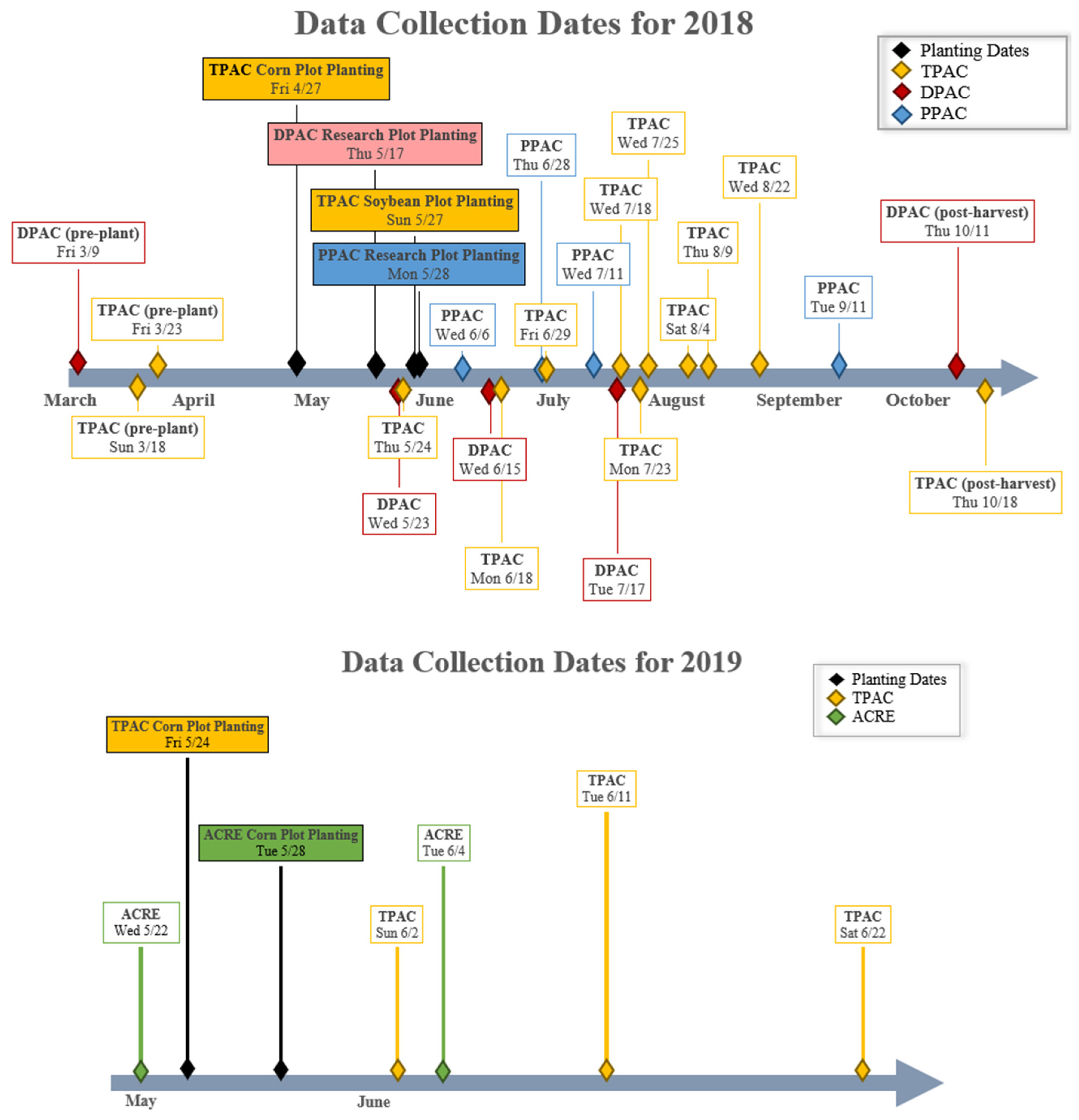
At PPAC, the most commonly found weeds within the research plot were dicot weeds, including giant ragweed (Ambrosia trifida), velvetleaf (Abutilon theophrasti), common lambs-quarters (Chenopodium album), and redroot pigweed (Amaranthus retroflexus). Monocot weeds at PPAC were predominately giant foxtail (Setaria faberi). At DPAC, the most common weeds within the research plot were tall waterhemp (Amaranthus tuberculatus), velvetleaf, and prickly sida (Sida spinosa). At TPAC, the most commonly occurring weeds found in the research plots were giant ragweed and redroot pigweed (Amaranthus retroflexus).
Monocot weeds commonly found in the research plots at TPAC were green foxtail (
Setaria viridis) and panicum (
Poaceae virgatum). At ACRE, common dicot weeds included giant ragweed. For the 2018 growing season at TPAC, the soybean research plot was planted on 27 May 2018. Planting began on the TPAC corn plots and the PPAC and DPAC corn and soybean research plots on 27 April, 28 May, and 17 May. A timeline of the UAS data acquisition dates over the 2018 growing season is shown in
Figure 1.
Data collection was also done during the first month of the 2019 growing season at ACRE and TPAC. Due to the high amount of rain received during the Spring of 2019, planting at these locations did not occur until late May. Planting at the TPAC and ACRE corn plots began on 24 May and 28 May, respectively. The timeline of the 2019 data collection is shown in
Figure 1.
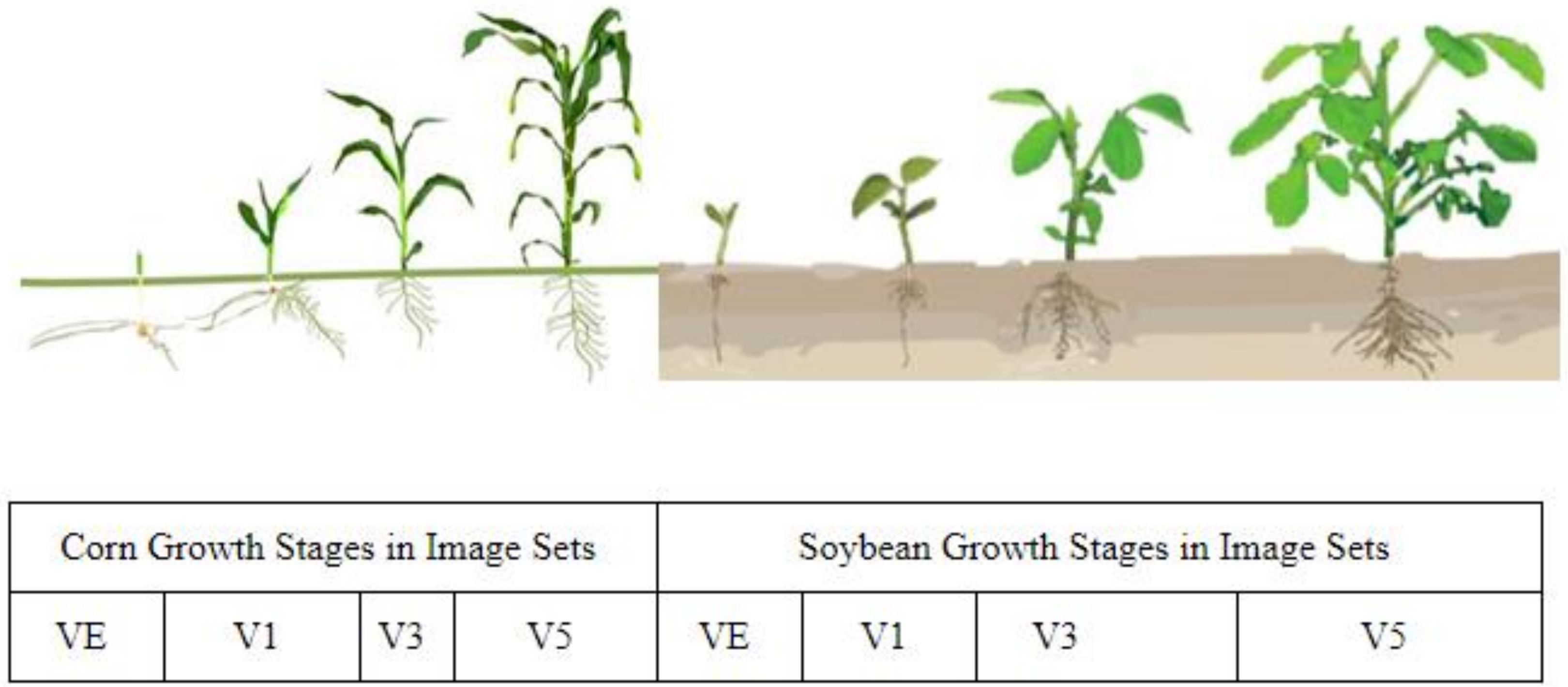
Research plot fields were rotated between corn and soybeans between the 2018 and 2019 growing seasons at TPAC. Therefore, the location of the study area moved down six research plots (to the west within the research field) for the 2019 planting season, due to a change in experimental layout and planting. Data collection at ACRE was done to increase the number of images for the 2019 growing season. Late planting and the research conclusion dictated the removal of DPAC and PPAC from the flights conducted in 2019, as neither location had planted plots when data collection was undertaken. The first location was flown on 22 May 2019. This was done during pre-plant (PP). The second plot location, flown 4 June 2019, had corn at the first vegetative (V1) growth stage. A further explanation of corn and soybean growth stages is given in
Figure 2, where growth stages from emergence (VE) to fifth vegetative state (V5) are visualized. VE refers to the stage where the corn plant breaks through the soil surface.
2.1. Network Architecture—YOLOv3
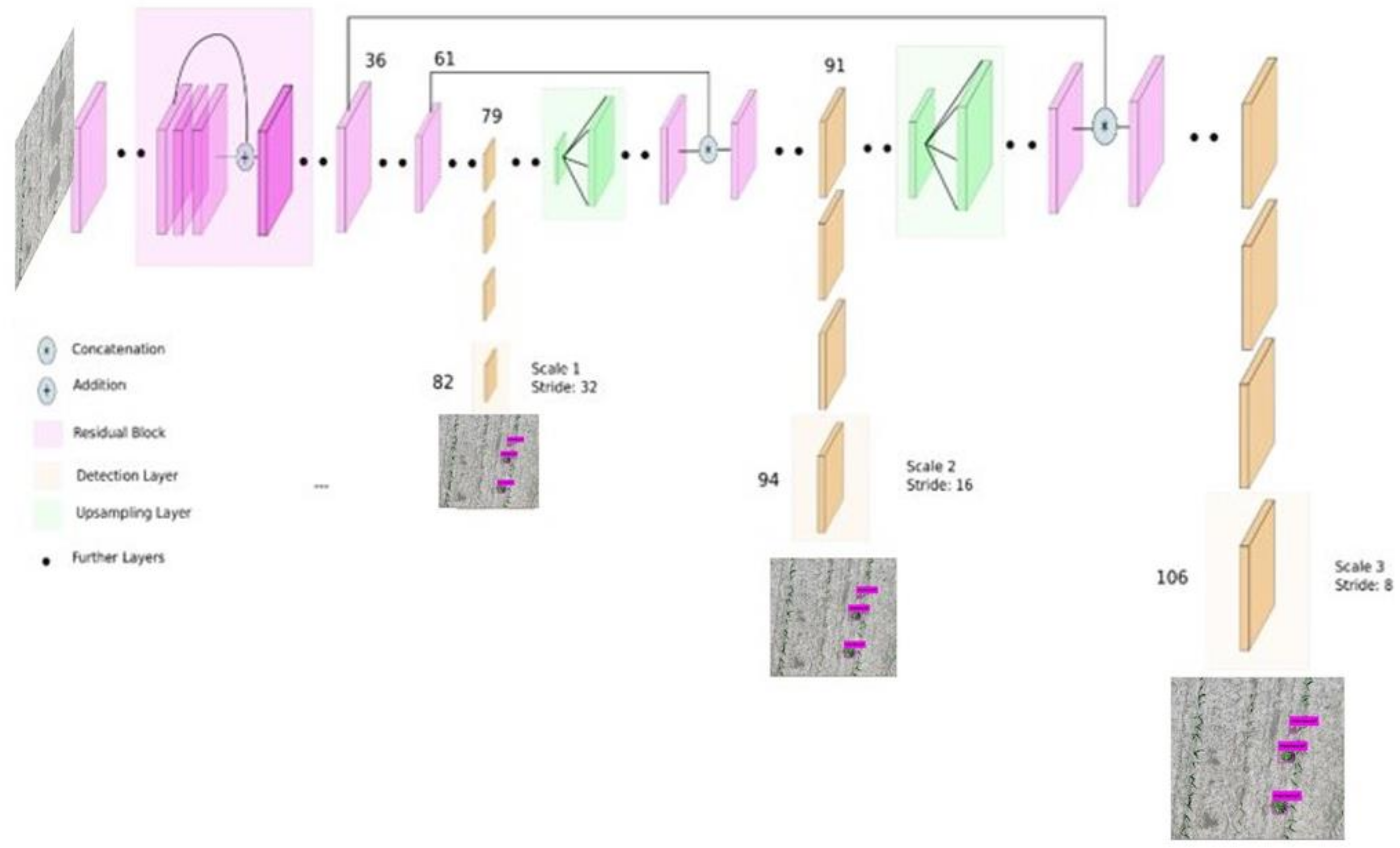
This research utilized an unmodified YOLOv3 network for weed detection from UAS images [
54]. In total, YOLOv3 consists of 106 layers. The initial 53 layers are called the network’s backbone, while the latter 53 are called the detection layers. An illustration of the YOLOv3 architecture is shown in
Figure 3.
The function of the first 53 layers is to extract features from the input images. These layers are based on an open-source neural network framework called Darknet [
54]. Hence, together, these layers are called Darknet53. The extracted features are used for detection at three different scales. These detections are then combined to get the final detection. The scale of plants in UAS images varies with changes in flight height and changes in the plant’s growth stage. Hence the multiscale detection of YOLOv3 is beneficial, especially for identifying monocot and dicot plants in UAS images.
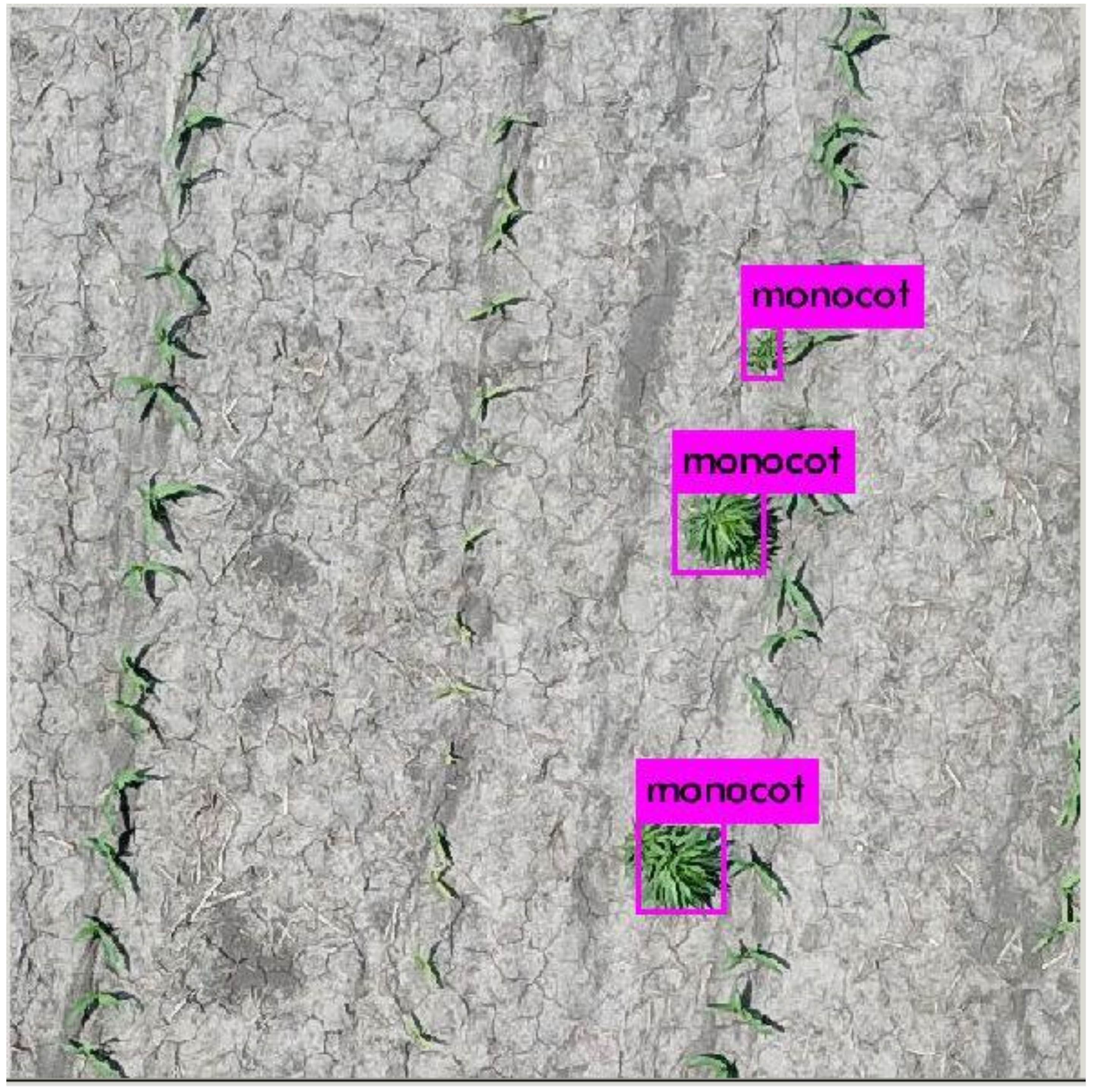
2.2. Labeling and Annotation of the Weeds Dataset
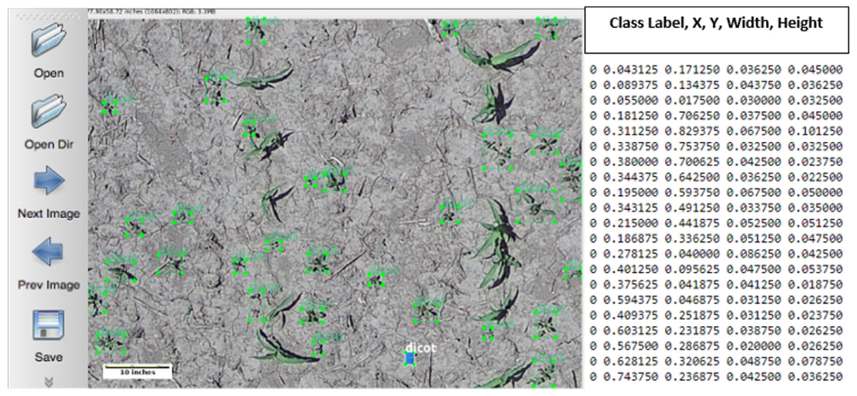
Images chosen for manual annotation were acquired during the 2018 (April through September) and early 2019 (May and June) growing season for the corn and soybean crops. Annotation refers to the physical creation of bounding boxes around a selected object. In contrast, a label refers to the name of the class (for example—monocot or dicot in this study) assigned to the annotation that is saved as metadata for the class file. Manual image annotation and labeling are tedious yet crucial steps in supervised learning. To train a network to detect each instance of an object, it must have a way to learn how the object looks and its position in relation to other objects within an image where detection is warranted. To accurately annotate and label the high-resolution UAS-based imagery collected, an image-editing tool with enough speed to label hundreds of weeds in an image and enhanced zoom features that focus on a particular region and clarity of the weeds present therein was required. After meticulous research and testing were performed, a labeling tool was finally found, LabelImg, which provided adequate labeling speed and user-friendly zoom and pan features [
56]. LabelImg converts each bounding box to five numbers. The first number corresponds to the class label. The second and third numbers correspond to the x- and y-coordinates of the center of the bounding box. Finally, the fourth and fifth numbers correspond to the width and height of the bounding box. An example of bounding box annotation using LabelImg is shown in
Figure 4 below.
Due to the amount of time required to complete manual annotation, speed and ease of use become increasingly important in the overall dataset creation workflow. A labeled RGB imagery dataset was created to train the weed detection model. RGB cameras were chosen as they are more affordable and more commonly used by farmers than other UAS-based sensors, such as multispectral or thermal ones [
57].
2.3. Methods for Choosing Imagery for Manual Annotation
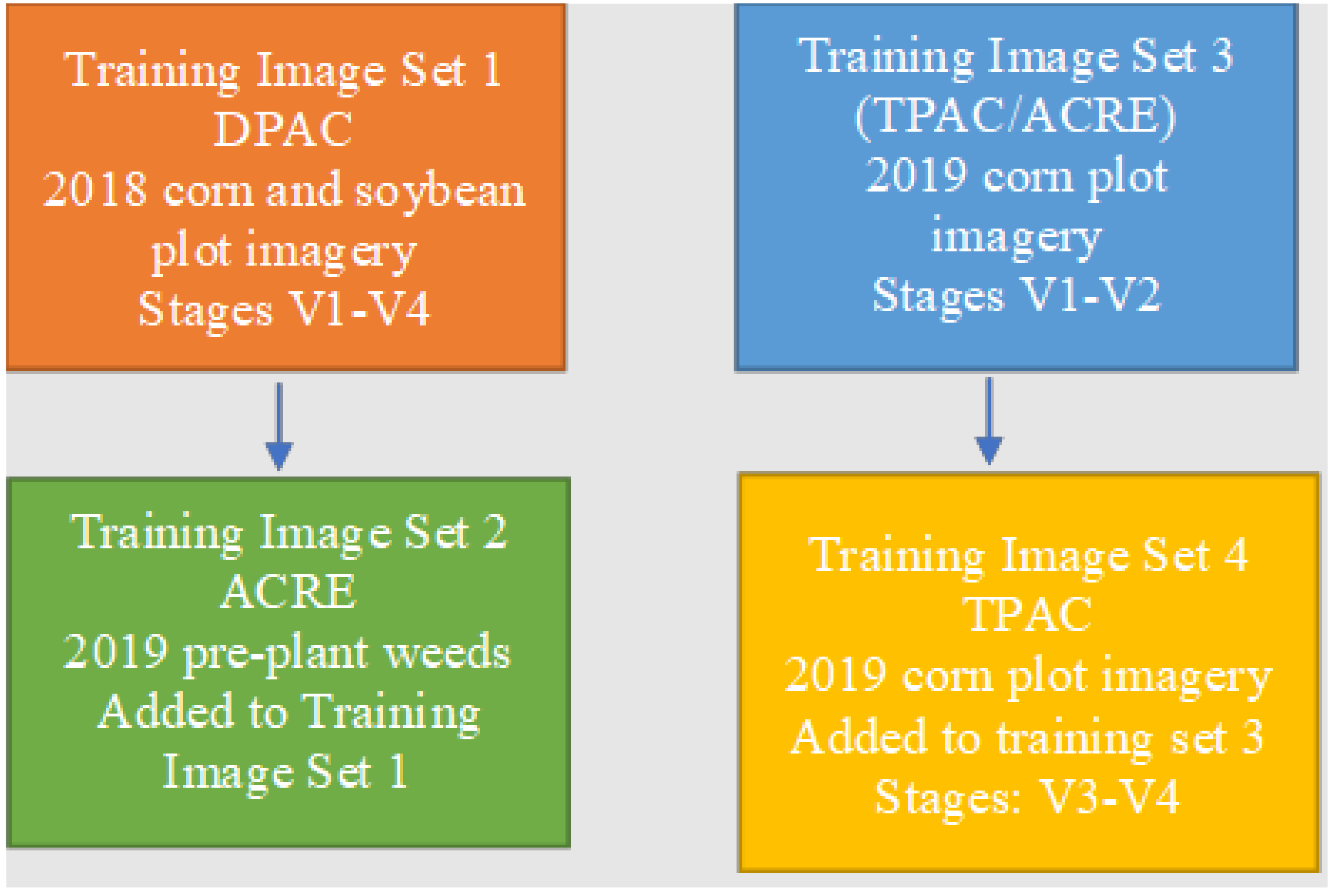
A total of 25 flights, each lasting approximately 24.5 min, were carried out in the 2018 and early 2019 growing seasons to acquire an average of 1113 RGB images per flight. While 27,825 RGB images were acquired in 2018 and 2019 combined, only 374 of these images were annotated for network training dataset creation. The reason for selecting a smaller percentage of total imagery data is because only early season and pre-plant imagery were chosen for manual annotation. Individual weed examples during later crop growth stages could not be used for annotation due to the difficulty of finding individual weeds within the imagery to be labeled. All of the later growth stage imagery had areas of heavy weed infestation, where weeds were clumped together. These images might be useful for other researchers and future network training, but the main focus of the reported research was on the early season, individual weed identification. A flowchart of the manually annotated training image set creation is shown in
Figure 5. Each set will be denoted as “Training Image Set #” to explain the training set creation methods better.
During the formation of Training Image Set 1, UAS-based weed imagery was acquired during the early growth stages of corn and soybeans in 2018 at 30 m AGL. For the creation of Training Image Set 2, 2019 pre-plant weed imagery was acquired at 10 m AGL and added to Training Image Set 1. Images of newly emerged to early-stage corn plots in 2019 were acquired at 10 m AGL for Training Image Set 3 to compare the differences between object detection performance on a multi-crop image set, such as Training Image Sets 1 and 2, to an image set from a single crop plot. There were no monocot weeds in this imagery, as no monocot weeds were present in this early growth stage imagery. This observation has been denoted as N/A in
Table 1. While configuring Training Image Set 4, early growth-stage corn plot imagery was acquired at 10 m AGL. No imagery was acquired from soybean plots during this time. Within these images, corn had fully emerged, and it was easier to decipher between weeds and crops. The criteria for identifying emerged corn included a longer average leaf length, larger average leaf diameter, a succinct spacing of corn plants based on planting pattern, and other physical traits, such as leaf structure [
58]. A weed-free image showing only corn was added to the training set for every monocot and dicot labeled image. A corresponding empty text file was also needed to inform the YOLO network that there were no labeled objects. This step ensured that there were as many negative samples [
59], i.e., images containing only non-desirable objects, as there are numbers of labeled images (positive samples).
2.4. Hardware and Software Setup for Deep Learning Network Training
An Alienware R3 laptop computer with a 2.8 GHz Core i7-7700HQ processor with 32 gigabytes (GB) of RAM was used to train the YOLOv3 network. A 6 GB NVIDIA GTX 1060 graphical processing unit (GPU) was installed on the laptop to enable deep learning network training. The Ubuntu operating system, version 18.04, was installed on the laptop. Ubuntu was disk partitioned to 200 GB, as it was set up to be dual booted alongside the Windows operating system already available in the computer. Access to Purdue University’s community supercomputer cluster allowed for network training at a larger scale. The Gilbreth cluster utilized for this training is “optimized for communities running GPU intensive applications such as machine learning.” The Gilbreth cluster is comprised of “Dell compute nodes with Intel Xeon processors and NVIDIA Tesla GPUs” [
60]. A detailed overview of the compute nodes and GPU specifications can be found in
Table 1 above.
2.5. Constraints in Training Image Set Creation
For the creation of Training Image Set 1, 100 UAS acquired RGB images from the 2018 early season corn and soybean fields were selected for dataset creation. These raw images were of size 4000 × 3000 pixels. Furthermore, images were acquired at 30 m AGL in a two-acre soybean plot surrounded by corn. The soybeans in these images were in the V1–V2 growth stage. The surrounding corn plots planted prior to the soybean plot were in the V3–V4 growth stage. Images were annotated using bounding boxes, and present weeds were labeled as either monocot or dicot. Before the bounding box annotations were created and labeled, images were resized to 416 × 416 pixels during preprocessing. A 1:1 aspect ratio was used per YOLOv3 network constraints. A total of 8638 weeds were annotated and labelled for an average of 86 weeds per image. Each weed was categorized as either monocot or dicot. Aside from allowing for quicker annotation, these two categories were chosen to provide a broader representation of weed types present in the field. Furthermore, the abundance of either weed type will require a different herbicide application to implement an effective weed management strategy. For example, certain herbicides, such as 2,4-D and Dicamba, are used to target dicot weeds. While they can be applied to monocot crops such as corn without damage, dicot crops such as soybean need to be tolerant to avoid harm [
61]. The YOLOv3 network reads a bounding box by the pixel location of its four corners within an image, allowing for the bounding box’s width and height to be normalized by the width and height of the resized image. Specifically, the x-center, y-center, width, and height are float values relative to the width and height of an image. The values of these indices were normalized between 0.0 and 1.0. In addition to resizing the images, anchor boxes were calculated based on the manually labeled bounding boxes, using the calc_anchors bash command. This command, built into the Darknet repository [
60], was used in this study. Anchor boxes were calculated through a k-means clustering technique, shown in Equations (1)–(5) below:
where,
,
,
, and
are the x coordinate, y coordinate, width, and height of the predicted bounding box, respectively;
,
,
, and
are the bounding box coordinate predictions made by YOLO;
and
is the top left corner of the grid cell that the anchor lies within; and
and
are the width and height of the anchor [
62].
,
,
, and
were normalized by the width and height of the image in which the anchor was being predicted. Finally,
outputs the box confidence score. Pr is the probability of a predicted bounding box containing an object, Pr(Object).
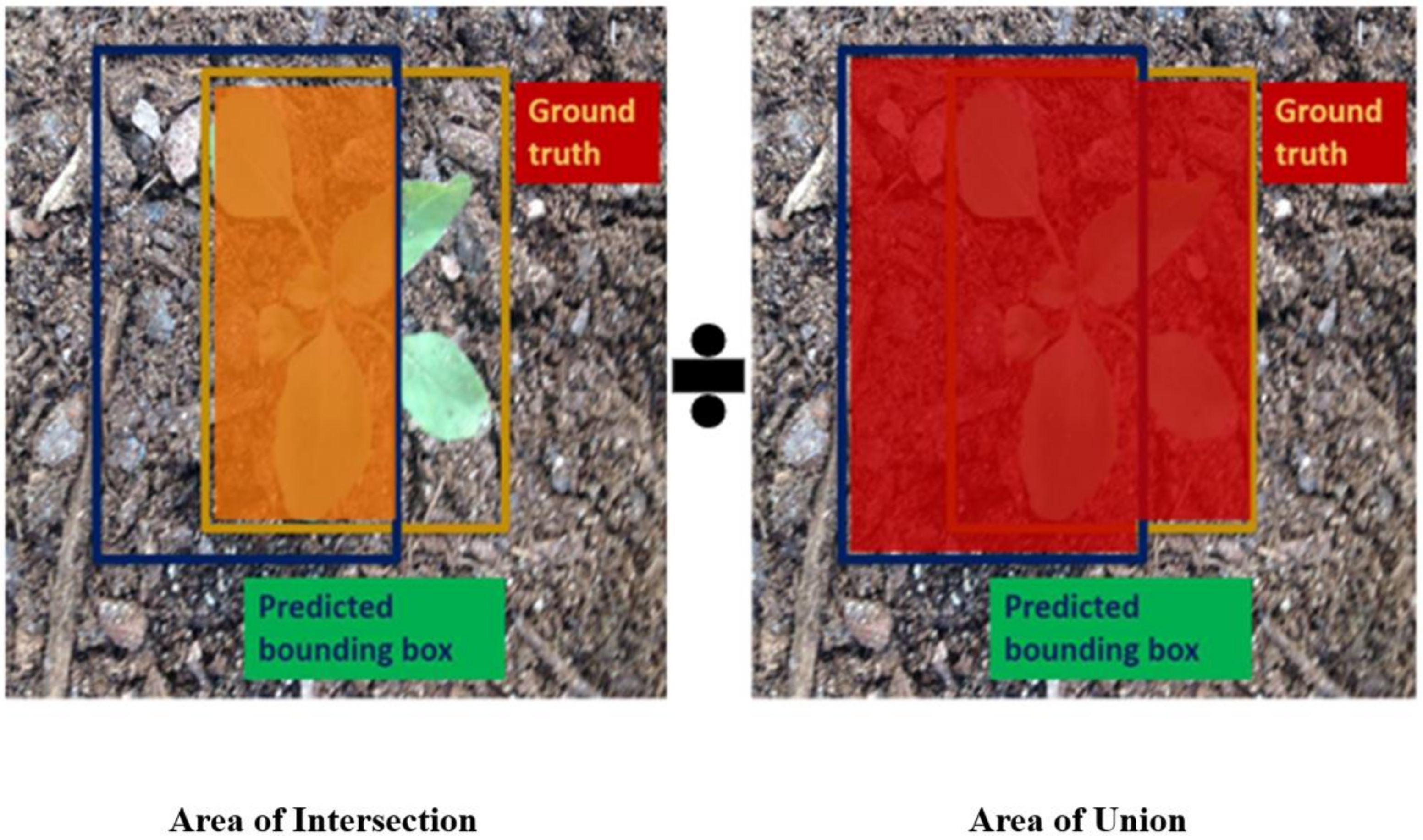
Training Image Set 2 added an additional 108 raw images of size 4000 × 3000 pixels of the 2019 pre-plant weed imagery. This imagery was taken at 10 m AGL. Training Image Set 2, therefore, comprised of imagery acquired at the height of 30 m and 10 m AGL. After the images were resized to 416 × 416 pixels, they were added to Training Image Set 1, making a total of 208 images in Training Image Set 2. After resizing, bounding box annotations were created for these images and labeled as either monocot or dicot. An additional 4077 monocot and dicot weeds were annotated and labelled, resulting in a total of 12,715 weed annotations. This gave an average of 61 weeds per image. The identified weeds were small dicots (less than five centimeters (cm) in diameter). Anchors were again calculated to ensure accuracy with the updated data, and the learning rate was modified from 0.01 to 0.001 in the configuration file. During this time, the training intersection over union (IoU) of the annotated vs. predicted bounding boxes was calculated to predict areas where a specific class of weed was present. The network calculated the predicted bounding boxes based on Equation (1). IoU is the ratio between the area of overlap and the area of union concerning the predicted (through network training) versus ground-truth (manually annotated) bounding boxes [
63]. An illustration of the IoU is shown in
Figure 6 below.
Computing the IoU scores for each detection allows a threshold, T, to be set for converting each calculated IoU score into a specific category. IoU scores above a given threshold are labeled positive predictions, while those below are labeled false predictions. Predictions can be further classified into true positive (TP), false positive (FP), and false negative (FN). A TP occurs when the object is present, and the model detects it, with an IoU score above the specified threshold. There are two scenarios in which an FP can occur. The first happens when an object is present, but the IoU score falls below the set threshold. The second occurs when the model detects an object that is not present. A FN happens when the object is present, but the model does not detect it. In essence, the ground-truth object goes undetected [
62]. Precision is the probability of predicted bounding boxes matching the ground-truth boxes. This is detailed in Equation (6).
where:
TP = true positives, FP = false positives, and precision = the true object detection overall detected boxes. Precision scores range from 0 to 1, with high precision implying that most detected objects match the ground-truth objects. For example, a precision score of 0.7 means a 70% match. Recall measures the probability of the ground-truth objects being correctly detected. This is shown in Equation (7).
where FN = false negatives and recall = the true object detection overall from the ground-truth boxes. The recall is also referred to as the sensitivity and ranges from 0 to 1 [
62]. After obtaining the precision and recall, the average precision (AP) and mean average precision (mAP) were calculated for each class and image set, as shown in Equations (8) and (9), respectively.
The mAP was calculated by dividing the sum of the APs for all classes by the total number of objects to be detected [
55].
For the creation of Training Image Set 3, the imagery was collected during the 2019 early season data collection missions. Altitude was set at 10 m AGL for these flights after poor object detection performance was observed for Training Image Set 1 and Training Image Set 2, consisting of images acquired at 30 m AGL and a combination of 30 m and 10 m AGL, respectively. This set comprises 100 raw images of size 4000 × 3000 pixels. As corn was the only crop planted during these data collection dates, corn plots were chosen to make up this dataset. Nearly all weeds present in these fields were dicot. Therefore, all bounding box annotations for the images were labeled as a dicot. For this training, a number of changes were made to the yolov3_weeds.cfg file. Image size was increased to 512 × 512, from 416 × 416 in the previous image set, to test whether resizing to a higher resolution would improve training accuracy. A total of 7795 dicot weeds were annotated and labelled in this set for an average of 78 weeds per image. It was found that image size could be increased by changing the network hyperparameters in the configuration file. Specifically, adjusting the batch and subdivision values to reduce the likelihood of a memory allocation error was experimented with. The learning rate was also modified from 0.001 to 0.0001. The network also recalculated Anchors using the calc_anchors command, which performs Equation (1). Before creating Training Image Set 4, a number of changes had to be made to increase the average precision, lower the false-positive rate, and introduce imagery with monocot weeds present. These steps were undertaken to test the network performance with two-class detection.
Training Image Set 4 contained 166 RGB images, acquired at 10 m AGL, from the V1–V4 growth stages corn fields. Additional raw images of size 4000 × 3000 pixels were collected from the 2019 early season corn fields of the V3–V4 growth stages. These were split into 20 smaller tiles instead of resizing the original image into a smaller pixel resolution. Each weed was manually annotated with bounding boxes and labeled either monocot or dicot. These image tiles were then resized from 894 × 670 to 800 × 800 pixels, matching the configured network size. Weeds within these image tiles were easier to identify and annotate. Creating bounding box annotations and labeling them took less time compared to original, non-split images. The number of weeds per image was significantly decreased as smaller sections of the original image were used. It is recommended that image size be as similar to the network parameter as possible while training [
64]. Sixty-six tiles from the split images, resized to 800 × 800 pixels, were chosen to be labelled and annotated. These were added to the 100 previously resized images used in Training Image Set 3. An additional 5147 monocot and dicot weed instances were annotated and labelled for a total of 12,945 weeds in Training Image Set 4. This also gave an average of 78 weeds per image for network training.
Access to Purdue University’s Gilbreth supercomputer cluster, optimized for GPU-intensive applications [
60], allowed for network training at a larger scale. Before the 2019 early season corn training set, Training Image Set 4, could be trained on the Gilbreth cluster, several changes needed to be made in the network configuration file, yolov3.cfg. The additional network training of 20,000 iterations for Training Image Set 4 on the Gilbreth cluster has been defined as Training Image Set 4+. These changes included setting the batch size to 64, subdivisions to 16, angle to 30, and random to 1. The angle hyperparameter allows for random rotation of an image over the training iterations by a specified degree, i.e., 30 degrees. This image augmentation has improved network performance and reduced loss [
65]. The random hyperparameter has also been reported to augment images by resizing them every few batches [
65]. For network training, the 50% detection threshold (T = 0.5) was used for Image Sets 1, 2, 3, and 4. At this value, only objects that are identified with a confidence value greater than 50% are considered [
54]. For Image Set 4+, the 50% threshold was again used along with the 25% detection threshold (T = 0.25). All other parameters remained the same in Training Image Set 4+ as in Training Image Set 4.
4. Discussion
Deep learning is quickly becoming popular among the research community for precision agriculture applications, including weed management. Identifying the weeds within a field can help farmers implement more efficient management practices. Image classification using DCNN has been gaining the attention of researchers for identifying weeds. However, as image classification can only identify single objects, its use on UAS acquired images at high altitudes can prove challenging to accurately identify multiple weeds within images. Nevertheless, the identification of weeds is of vital importance as locating the weeds within fields is necessary to ensure effective SSWM. Therefore, object detection was used in this study to identify and locate multiple weeds within UAS-acquired images. By identifying and locating the weeds, regions of the field consisting of weeds can be targeted by farmers for herbicide application, resulting in reduced costs, reduced negative environmental impacts, and improved crop quality.
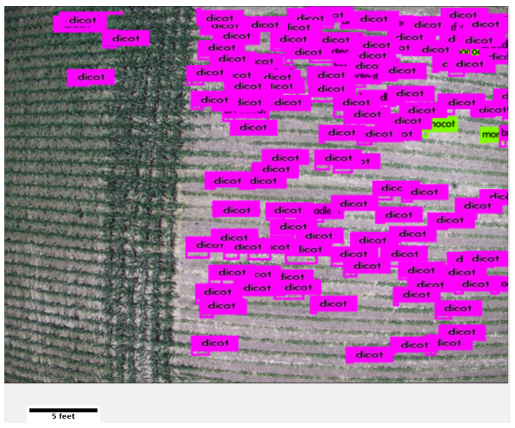
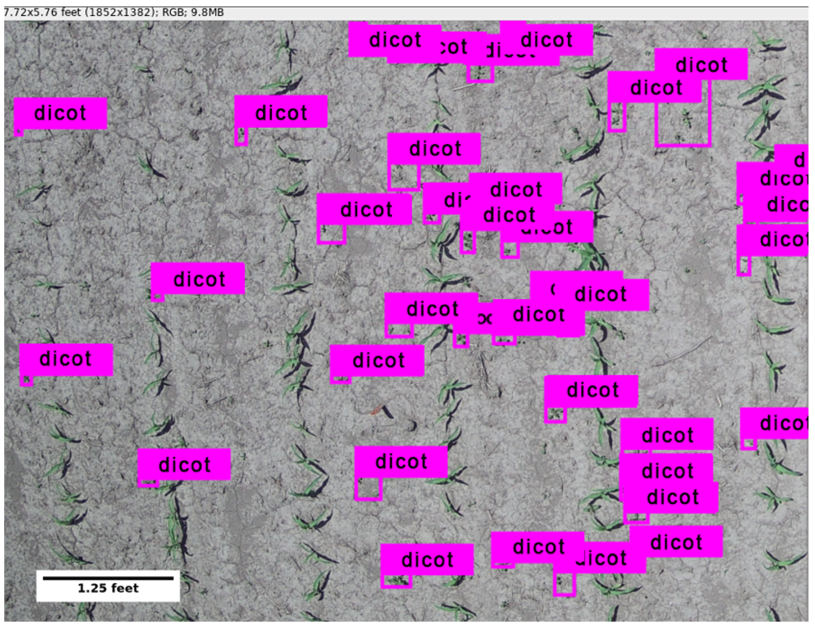
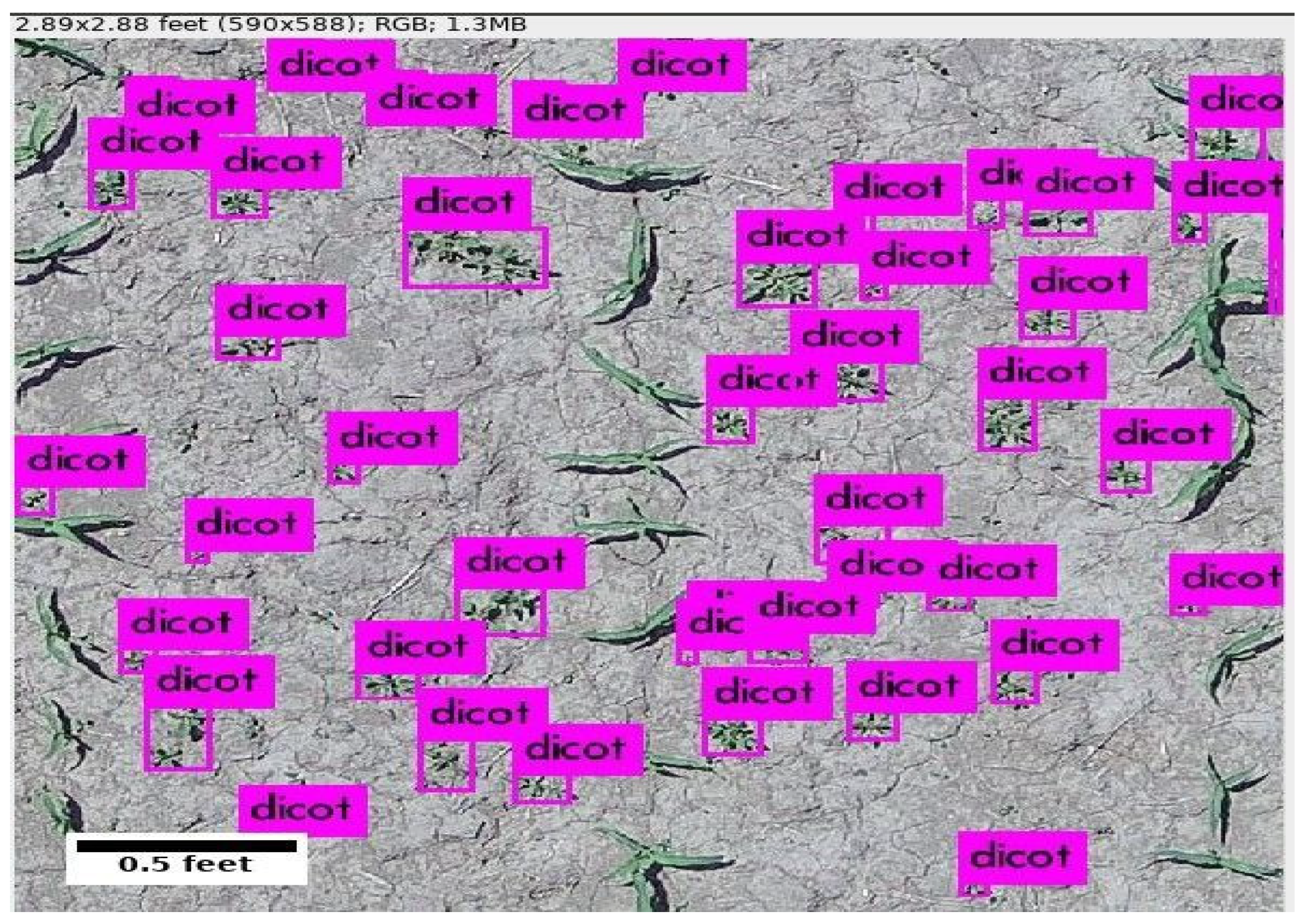
This study used deep learning-based object detection to identify and locate weeds. Although object detection may be implemented using multiple different DCNN-based algorithms, YOLOv3 was selected due to the fewer parameters needed for faster training, inference speed, and high detection scores for fast and accurate weed identification and localization. This network was particularly helpful in detecting multiple instances of weeds, especially when the neighboring emergent crops were of similar color and size. For example, in Training Image Set 4+,
Figure 11 showed that the network could detect over 40 instances of dicot weeds in a single image. Moreover, YOLOv3 has fewer parameters than its predecessors, which keeps the model size at around 220 MB. Compared to other object-detection networks, such as Faster R-CNN, whose model size is over 500 MB [
41], the smaller size translates into faster inference and the ability to run on resource-limited computing devices, such as Raspberry Pi or NVIDIA Nano.
In summary, this research resulted in four training image sets of early-season monocot and dicot weeds in corn and soybean fields acquired at heights of 30 m and 10 m AGL using a UAS. The impact of height on UAS imagery was evident as images acquired at lower heights resulted in more accurate results. The models trained for each image set were compared using different evaluation metrics. However, AP was used as the primary evaluation metric based on the practices present in the current literature. Through improvements in image set creation and training methods, a significant improvement was made to the object detection average precision at each successive stage. It was found that training time was significantly faster on the Gilbreth cluster than locally, using a GPU-enabled laptop. For example, a training time over 20,000 iterations took 108 h to complete on the laptop for Training Image Set 4. This same dataset with the same specifications took 62 h to complete for 20,000 epochs on the Gilbreth cluster, defined as Training Image Set 4+.
After training the YOLOv3 model for each training image set, the results were compared and reported using AP and mAP scores. The mAP scores for the training image set results are specific to the 50% and 25% IoU thresholds (T = 0.5 and T = 0.25), as denoted in each respective table. For Training Image Set 1, images were acquired at 30 m AGL. This leads to a lower spatial resolution, making it harder for the network to detect monocot and dicot weeds. This was observed when low true positives, high false positives, low AP, and low mAP were reported. Hence, a mix of images acquired at 10 m and 30 m AGL was used for Training Image Set 2 to evaluate whether adding higher resolution images acquired from 10 m AGL helps make the network more robust. As is apparent from the results, a significant increase was not observed—the mAP score decreased by ~0.5%. Training Image Set 3 was then acquired from a height of 10 m and was used exclusively to detect the dicot weeds in the corn field, leading to an increase in the AP score. However, the increase was not significant as only a single weed type was identified, which resulted in identifying all plants, and ultimately a high FP rate was observed. Having learned that images collected from 30 m AGL does not provide enough spatial information for the network to train adequately, only images collected from a height of 10 m AGL were used in the final image set, Training Image Set 4. The network was trained for another 20,000 iterations on the same image set, leading to an increased network performance on par with the literature. The final training for Training Image Set 4+ led to the highest network performance with an AP @ 0.5 of 65.37% and 45.13% and AP @ 0.25 of 91.48% and 86.13% for monocots and dicots, respectively. This resulted in a mAP @ 0.5 of 55.25% and mAP @ 0.25 of 88.81%. This was close to the expected performance of YOLOv3, where for the MS COCO dataset, a mAP @ T = 0.5 score of 57.9% was reported [
46]. Furthermore, network performance increased when the images were resized to a higher 800 × 800 pixels for Training Image Sets 4 and 4+. The performance was comparable to recent weed studies, which utilized object detection for weed identification. Recently, the authors in [
45] identified weeds with total mAP scores of 22.7%, 25.1%, 17.1%, and 28.9% for Faster RCNN with ResNet50, ResNet101, InceptionV2, and InceptionResNetV2 feature extractors, respectively. Additionally, mAP @ T = 0.5 of 48.6%, 51.5%, 40.9%, and 55.5% were reported.
Recently, a new object-detection network belonging to the YOLO family was released. The network is called YOLOv4 [
64]. YOLOv4 uses the Cross Stage Partial (CSP) Network in addition to Darknet53 for feature extraction [
66]. The primary advantage of CSP is a reduction in computations by almost 20% while being more accurate on the ImageNet dataset when used as a feature extractor. The evaluation of Yolov4 for identifying and locating weeds in UAS images will be explored in future studies.
5. Conclusions
This study has demonstrated that training manually annotated and labeled monocot and dicot class image sets on the YOLOv3 object detection network can yield promising results towards automating weed detection in a row-crop field. This study has also demonstrated the feasibility of utilizing high-resolution, UAS-based RGB imagery to train an object detection network to an acceptable accuracy. A dataset of 374 annotated images, 27,825 raw RGB images, and the final training weight files from each training has been made publicly available on GitHub. It can be concluded that an annotated image set should be created for specific crops in which detection is to be performed. This was shown in Training Image Sets 3 and 4. Compared to the first two sets that mixed corn and soybean crops, the average precision improved significantly when single crop imagery was used. For example, unique image sets should be created for corn and soybeans separately. This will reduce the number of false positives from the resulting network training. It was also found that as many negative samples (non-labeled images) should be added to an annotated training set as positive samples (labeled images). The negative samples should not contain any objects that are desired for detection. By acquiring UAS imagery at the height of 10 m AGL, a significant improvement in YOLOv3 object-detection performance was observed for the creation of the training image sets for monocot and dicot weed detection, with an improved AP at both the T = 0.5 and T = 0.25 levels. After obtaining these promising results, we conclude that deep learning-based object detection is helpful for identifying weeds with field images using UAS for SSWM, especially early in the growing season.
Future research will first involve increasing the annotation and classes for object detection to reduce the false-positive rate. The trained models will then be moved towards a real-time, UAS-based weed detection system. This can be achieved by installing a microcomputer, such as a Raspberry Pi or NVIDIA Nano to the UAS, interfacing with the camera collecting the imagery, and installing a lighter memory version of YOLO, such as TinyYOLO, to the microcomputer. The final trained weights (the results of completed network training) can be loaded onto the microcomputer, and a bash script can achieve real-time video detection testing.
The future scope of this research will also include determining the effect of spatial and radiometric resolution on the accuracy of weed identification and localization [
3]. A systematic study could be conducted that determines the effect of UAS flight height on the accuracy of weed detection. It would help develop a recommendation on the optimal flight height for weed detection in practical applications. Moreover, a study could be conducted to establish the generalization accuracy of the YOLO network for weed detection over changing weather conditions in the field, as it would reduce the need for radiometric calibration [
67].


