Hydrometeor Classification of Winter Precipitation in Northern China Based on Multi-Platform Radar Observation System

Abstract

Hydrometeor classification remains a challenge in winter precipitation cloud systems. To address this issue, 42 snowfall events were investigated based on a multi-platform radar observation system (i.e., X-band dual-polarization radar, Ka-band millimeter wave cloud radar, microwave radiometer, airborne equipment, etc.) in the mountainous region of northern China from 2016 to 2020. A fuzzy logic classification method is proposed to identify the particle phases, and the retrieval result was further verified with ground-based radar observation. Moreover, the hydrometeor characteristics were compared with the numerical simulations to clarify the reliability of the proposed hydrometeor classification approach. The results demonstrate that the X-/Ka- band radars are capable of identifying hydrometeor phases in winter precipitation in accordance with both ground observations and numerical simulations. Three particle categories, including snow, graupel and the mixture of snow and graupel are also detected in the winter precipitation cloud system, and there are three vertical layers identified from top to bottom, including the ice crystal layer, snow-graupel mixed layer and snowflake layer. Overall, this study has the potential for improving the understanding of microphysical processes such as freezing, deposition and aggregation of ice crystal particles in the winter precipitation cloud system.

1. Introduction

The identification of hydrometeor particles in winter precipitation is critical for understanding microphysical processes in the cloud-precipitation system. The associated origins are generally agreed upon as dendritic ice crystal growth zones [1,2,3], plate crystal growth [4], ice particle density and shape modulations caused by riming and crystal aggregation [5], hydrometeor melting [6], and near-surface refreezing of either rain or freezing rain into sleet [7]. A weather radar, especially a dual-polarization radar, presents potential in the classification of hydrometeor particles [8]. Straka et al. [9] and Holler et al. [10] applied the empirical Boolean decision logic approach to classify hydrometeors with the consideration of differential reflectivity ($Z_{DR}$), linear depolarization ratio ($LDR$) and the height of melting layer in hailstorm. With the update of Weather Surveillance Radar-1988 Doppler (WSR-88D), the fuzzy logic method is widely used for hydrometeor identification [11,12,13,14,15,16]. However, Kurdzo et al. [17] reported a limitation of using the fuzzy logic algorithm in the recognition of non-meteorological echoes (e.g., biological and ground clutter). It is also known that the existing hydrometeor classification methods fail to recognize the refreezing issue in winter precipitation [18]. According to the microphysical theory, and previous observational studies, Thompson et al. [19] proved that a fuzzy logic classification method, based on polarimetric variables, can identify the discrimination of the area, consisting of wet snow, aggregates, plates, dendrites or other small ice crystals. The evaluation of hydrometeor classification retrievals seems to be improved at shorter wavelengths (e.g., X-band). However, it has yet to be fully addressed.

Reinking et al. [20] concluded that measurements of depolarization with a Ka-band dual-polarization radar provide effective estimates of hydrometeor identity to separately distinguish drizzle, pristine crystals of various growth habits, graupel, and aggregates in winter storm clouds. Shupe [21] proposed an algorithm for identifying the hydrometeor phases and shapes based on the joint observation of an 8 mm cloud radar, laser radar and microwave radiometer. In addition, Khain et al. [22] suggested that the reflectivity threshold of mixed-phase cloud with ice crystals and supercooled liquid water is −30 dBZ, and the Doppler power spectrum of millimeter wave cloud radar (MMCR) is bimodal with a wide spectrum. However, the cloud with a single particle (e.g., ice crystal or supercooled liquid water) has a narrow spectrum [23]. Thus, spectral width is used to examine the mixed-phase cloud. Based on reflectivity ($Z$) and $LDR$, Liu et al. [24] determined the liquid water area in the cloud. Chen et al. [25] investigated the area with supercooled liquid water in the winter precipitation system and pointed out that the area of supercooled droplets in the cloud can be determined by the $Z$, $LDR$ and radial velocity ($V$). Based on the Doppler spectrum from the cloud radar, Li et al. [26,27,28] constructed an algorithm to identify supercooled cloud droplets, ice crystals and snowflakes. Furthermore, a snowfall case was investigated by identifying the spectrum peaks of the global spectrum, and spectrum moment parameters such as $Z$, $V$ and spectral width ($S_w$) for different particle categories were also provided [29]. Generally, most hydrometeor classification results are based on a reasonable inference, but lack sufficient clarification with regard to the cloud particle property in the observed precipitation system.

For a particle diameter of less than 200 μm, MMCR offers more details in winter precipitation compared with the dual-polarization radar. However, for larger cloud particles, a dual-polarization radar, especially X-band (herein XPOL), provides better detection in particle shape and spatial orientation as radar signals are dominated by the largest particles in the sampling volume. To this end, relevant information about the distribution of sizes, orientations, shapes, and diversity of hydrometeors within a particular radar sample volume can be derived from differential reflectivity ($Z_{DR}$), correlation coefficient (${\rho }_{HV}$), and the specific differential phase ($K_{DP}$) [8,9]. Both $Z_{DR}$ and $K_{DP}$ are positive (negative) for horizontally (vertically) aligned hydrometeors and have a value of zero for spherical particles, including those that effectively appear spherical to a radar because of excessive canting or tumbling. For a given oblate particle, both $K_{DP}$ and $Z_{DR}$ increase with ice or liquid water content, though only $K_{DP}$ is inversely proportional to radar wavelength. $Z$ also provides an indication of hydrometeor size and concentration. For graupel and snow, there is a difference in spatial arrangement, however, it is difficult to effectively classify them from $Z$,$V$, $S_w$ and $LDR$ using a single MMCR. If XPOL provides $Z_{DR}$ and the correlation coefficient (${\rho }_{HV}$), it is easier to distinguish. It means the combination of XPOL and MMCR has the potential of providing more information for particles with different sizes, spatial orientations and phases.

Since it is difficult to classify and verify the phases of various hydrometeor particles in winter precipitation cloud, especially on the radar beam level [18,19], a jointly multi-platform radar observation network, including ground-based equipment (e.g., XPOL, MMCR, microwave radiometer, etc.) and airborne sensors, was designed in this study. Based on the multi-platform radar observation network, we investigated the hydrometeor characteristics of 42 snowfall cases in a mountainous region of northern China from 2016 to 2020. The phases of hydrometeor particles and corresponding detection ranges of radar variables were comprehensively investigated. In addition, a fuzzy-logic hydrometeor classification algorithm was established based on the variables of, XPOL, MMCR and auxiliary temperature information.

The remainder of this study is organized as follows: Section 2 introduces the data and Section 3 describes the details of the identification algorithm. Comparisons of hydrometeor classification results are demonstrated in Section 4 and Section 5, based on a multi-platform radar observation system and numerical simulation. Conclusions and the discussion are provided in Section 6.

2. Data

The details of the multi-platform radar observation system are summarized in

Table 1. Details of multi-platform radar observation system in this study.

Instruments	Observed Parameters	Spatial and/or Temporal Resolution	Data Usage
MMCR	$Z$, $V$, $S_w$, $LDR$	30 m, 0.5 s	All the parameters are used for hydrometeor classification
XPOL	$Z$, $Z_{DR}$, $K_{DP}$, ${\rho }_{HV} V$, $S_w$	PPI: 150 m, 5 min RHI vertical resolution of 100 m (over the MMCR), 1 min	$Z_{DR}$, $K_{DP}$ and ${\rho }_{HV}$ are used for hydrometeor classification
Microwave radiometer	Total water vapor volume, total liquid water volume, and profiles of temperature, humidity, water vapor, and liquid water	1 min	Temperature and total liquid water volume are used for hydrometeor classification as the auxiliary parameters
Snow particle imager (SPI)	Shape and variation characteristics of surface precipitation particles	30 min	Ground measured particles used for hydrometeor classification
Airborne equipment 3V-CPI	Particle images within the range of 10–1280 μm	2D-S: 9–11 μm CPI: 2.3 μm	Hydrometeor classification verification
Airborne equipment HVPS-3	Larger particle images within the range of 150–19,200 μm	150 μm	Hydrometeor classification verification
Airborne equipment AIMMS-20	Temperature, humidity, air pressure, horizontal and vertical wind speed	1 s	Hydrometeor classification verification and temperature parameter correction

. Bejing time, i.e., UTC+8, is used in this study.

The details of the multi-platform radar observation system are presented in Figure 1. Figure 1a shows the topographic map around the Yanjiaping (YJP) observation station (115.73° E, 40.52° N, 1344 m), located 6 km southwest of Haituo mountain. The station was built in 2014 and equipped with XPOL, MMCR, microwave radiometer, automatic weather station, snow particle imager (SPI), weighing gauges, present weather sensor (OTT) and 2D-video-distrometer (2DVD). Figure 1b,c shows the XPOL radar located 24 km southeast of YJP station. Figure 1d shows the Kingair aircraft measurement platform. With the continuous range-height-indicator (RHI) scanning, XPOL takes the location of MMCR in the YJP observation station as the scanning angle. A complete RHI scanning cycle requires 1 min. The time-height-indicator (THI) mode was used for MMCR, to obtain vertical macro- and micro-characteristics of the winter precipitation cloud system. Additionally, the vertical in situ measurement was performed with the Kingair aircraft across the observation range of MMCR, which helps obtain the hydrometeor particle images and meteorological elements within the ground radar’s observation range.

3. Methods

3.1. Data Processing Method for X- and Ka-Band Radars

The RHI and THI modes were used in XPOL and MMCR, respectively. With the temporal resolution of 1 frame per minute, the vertical resolution of XPOL was 100 m. The MMCR features the temporal resolution of 16 frames per second and its vertical resolution is 30 m. In order to create spatially temporally consistent datasets for the XPOL and MMCR radars, the spatiotemporal resolution of $Z$, $Z_{DR}$, $K_{DP}$ and ${\rho }_{HV}$ in XPOL was interpolated to match the MMCR data. Firstly, the height difference of the two radars were corrected with the geographic information of XPOL and MMCR to match the same area observed, and then the spatial resolution of XPOL data in the vertical direction was interpolated to be the same as MMCR, after which the XPOL data were unified to match the temporal resolution of MMCR.

3.2. Attenuation Correction Method for the MMCR Reflectivity

Due to the importance of $Z$ in the hydrometeor classification algorithm, attenuation correction of $Z$ (MMCR) is required. A reverse correction method is proposed based on the relationship between $Z$ and surface snowfall, i.e., S (Equations (1) and (2)). Additionally, the correction of path attenuation was performed using Equation (3). Because attenuation in dry snow measurement could be ignored, $Z$ from XPOL was close to observation.

The Z-S equation is as follows:

$$Z=a{S}^b$$

(1)

where $a$ and $b$ are constant coefficients, the unit of $Z$(MMCR) is mm⁶·m⁻³, $S$ represents liquid-water-equivalent snowfall (unit: mm·h⁻¹). The coefficients a and b are retrieved according to the assumption that the aggregate snowflake aspect ratio was assumed to be 0.6 and terminal fall velocities were calculated at a certain V-D relation [30]. Here, $a$ and $b$ are assumed to be 56 and 1.2, respectively [30,31]. Equation (1) is thus simplified as follows:

$$S=0.0349·{10}^{0.0833·Z}$$

(2)

where the units of $Z$ and $S$ are dBZ and mm·h⁻¹, respectively. Battan [32] indicated that under Rayleigh scattering, the attenuation of dry snow to $Z$ is related to snowfall amount and radar wavelength. The equation could be expressed as follows:

$$k_{Dry-snow}=0.035S^2{\lambda }^{-4}+0.0022S{\lambda }^{-1}$$

(3)

where $k$ is the attenuation rate (unit: dB·km⁻¹), and $\lambda$ stands for wavelength (unit: cm). In Equation (3), the first and second terms describe the attenuation caused by volume scattering and absorption, respectively [33]. The estimations are evaluated by mean standard deviation (MSD) and ρ, and MSD is defined as follows.

$$MSD=\left\{{\left[{\displaystyle \sum }_{i=1}^N{(S_G-S_Z)}^2\right]}^{1/2}/{\displaystyle \sum }_{i=1}^N{S}_G\right\}\times 100\%$$

(4)

where $S_G$ (mm·h⁻¹) is the snowfall measured by surface weighing gauges, and $S_Z$ (mm·h⁻¹) is the snowfall estimated by $Z$.

The snowfall comparison shown in Figure 2 implies that both hourly and accumulated snowfall estimations performed well with the observation after attenuation correction on 29 November 2019 from 14:00 to 02:00 the next day. Thus, an 8 dBZ correction of the MMCR echo was employed to compensate for systematic bias and attenuation.

Due to the low level of snowfall and thin echo, the attenuation rate is 0.165 dB/km with the maximum as 1.43 mm·h⁻¹ from 17:48 to 18:48 on 29 November 2019, and the attenuation along the whole path was less than 0.66 dBZ. Compared with XPOL reflectivity in Figure 3c, both the value and spatiotemporal distribution of the echoes with the MMCR reflectivity correction were found to be similar to the XPOL reflectivity. Additionally, the time series of echoes from the two radars at different heights are shown in Figure 4. It also shows a comparison between the XPOL and MMCR reflectivity at different heights from 17:48 to 18:48 on 29 November 2019. MMCR reflectivity after attenuation correction was consistent with XPOL reflectivity, especially at the heights of 1000 m, 1500 m and 2000 m. The MMCR reflectivity was found to be smaller below the height of 500 m, and the corrected MMCR reflectivity is 2.5 dBZ lower than the mean XPOL reflectivity.

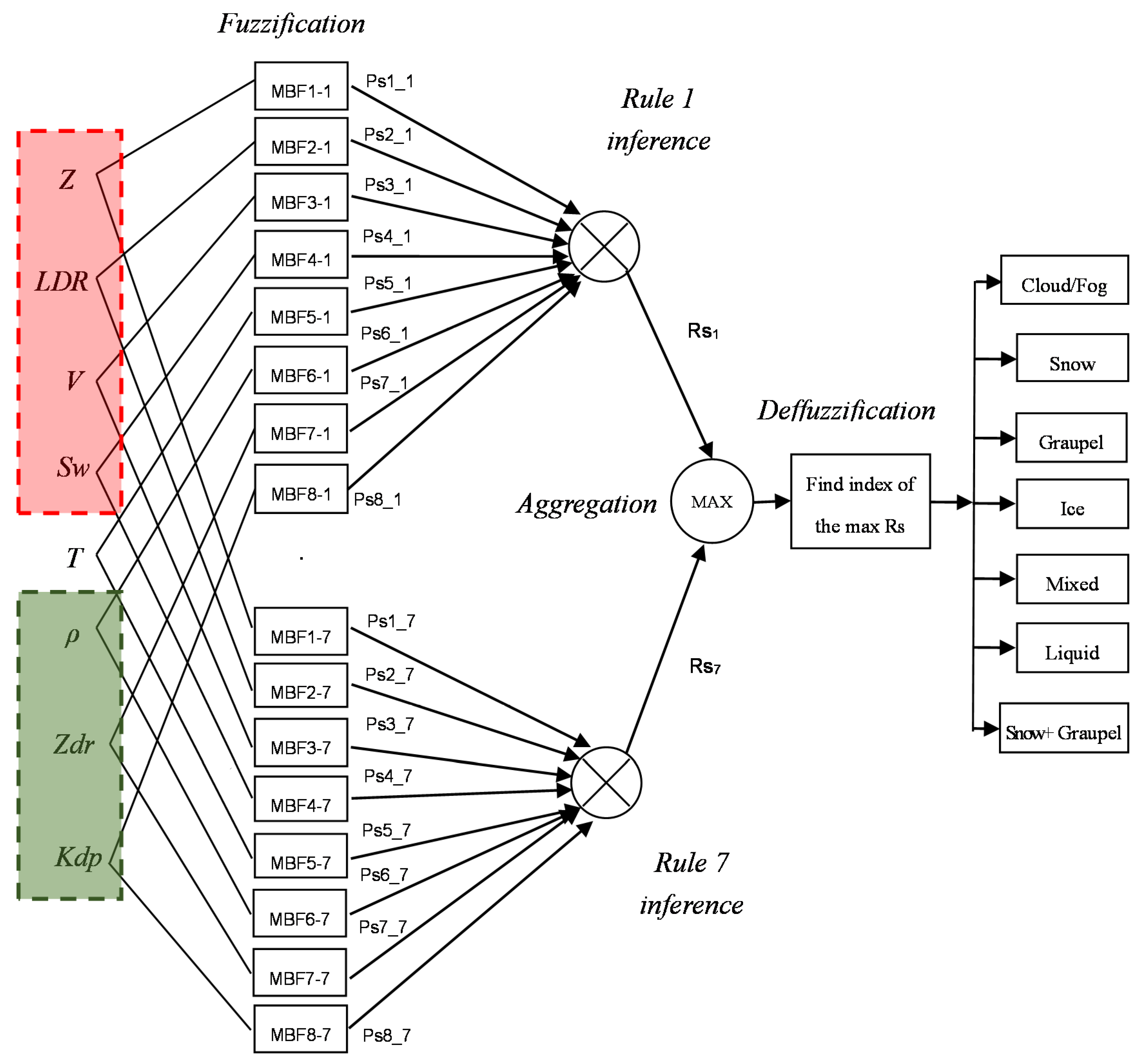
3.3. Phase Classification Method

The fuzzy logic method was used to classify the hydrometeor particle phases in the winter cloud precipitation system (Figure 5).

Firstly, the phases of hydrometeor particles observed near the surface with the SPI and the corresponding ranges of detection parameters from both XPOL and MMCR are summarized. More details are provided in Section 3.4.

Secondly, the $\beta$ function in Equation (5) was used as the membership function.

$$\beta \left(x,m,a,b\right)=\frac{1}{1+{\left[\raisebox{1ex}{$x-m$}\!\left/ \!\raisebox{-1ex}{$a$}\right.\right]}^{2b}}$$

(5)

where $a$ represents the width of function, $b$ represents the slope, $m$ is the central point of the function, and $x$ is the variable input. Taking $Z$ as input, the $\beta$ function corresponding to each category of hydrometeor particle was calculated, as shown in Figure 6. In both steps, normalized parameter fields were evaluated in the fuzzy logic algorithm through “membership functions”, which are the curves for each parameter that map each matrix point to the “membership value” between 0 and 1.

Thirdly, the inference was performed and compounded to obtain the total rules set:

$$R{\mathrm{s}}_j={{\displaystyle \sum }}_{i=1}^8{A}_i^{j}P{s}_{i-j}$$

(6)

where $A_i^j$ represents the weight coefficient of No.$i$ input to $P{s}_{i-j}$, $j$ stands for the particle phase, and $P{s}_{i-j}$ is the fuzzy value, $A_i^j$ is calculated according to radar data quality, characteristics and the importance in hydrometeor-type classification. The weight coefficient for each parameter is generally set according to two aspects: the meanings of the parameters and the reliability of the parameters. Firstly, we set each parameter with an initial value of 0.5, and then increased or decreased the weight coefficient by 0.1 according to the meaning and reliability of the parameters. Where $Z$ and ${\rho }_{HV}$. $Z$ represents the size and number concentration of particles in the sampling volume, which has high reliability after the attenuation correction and verification, while ${\rho }_{HV}$ represents the particle uniformity. If the particles are mainly the same in the sampling volume, the ${\rho }_{HV}$ is larger, and many categories of particles can be distinguished, so the weight coefficients of $Z$ and ${\rho }_{HV}$ both increase by 0.1. Both $LDR$ and $Z_{DR}$ are parameters that describe the shape of particles, and they play a relatively small role in the classification of snow and ice crystals. The weight coefficient will be reduced by 0.1. Furthermore, $V$ is related to particle phase and particle diameter, and $S_w$ is related to particle type and motion consistency in the sampling volume, and the weight coefficient will not change. $K_{DP}$ depends on the size of the raindrop deformation, and is negligibly affected by snow, ice crystals, and grauple, so the weight coefficient will be reduced by 0.2. A long period of surface observation data is beneficial for the preliminary adjustment of the algorithm and the identification results in different weight coefficients, verified from the surface observations. Finally, the $A_i^j$ values of $Z$, $LDR$, $V$, $S_w$, $T$, $Z_{DR}$, $K_{DP}$ and ${\rho }_{HV}$ are set as 0.6, 0.4, 0.5, 0.5, 0.6, 0.4, 0.3 and 0.6, respectively.

The phase for each particle ($R{s}_j$) is then transformed from the composite results. Comparing the $R{s}_j$ values, the index $j$ corresponding to the maximum value is identified as the hydrometeor type.

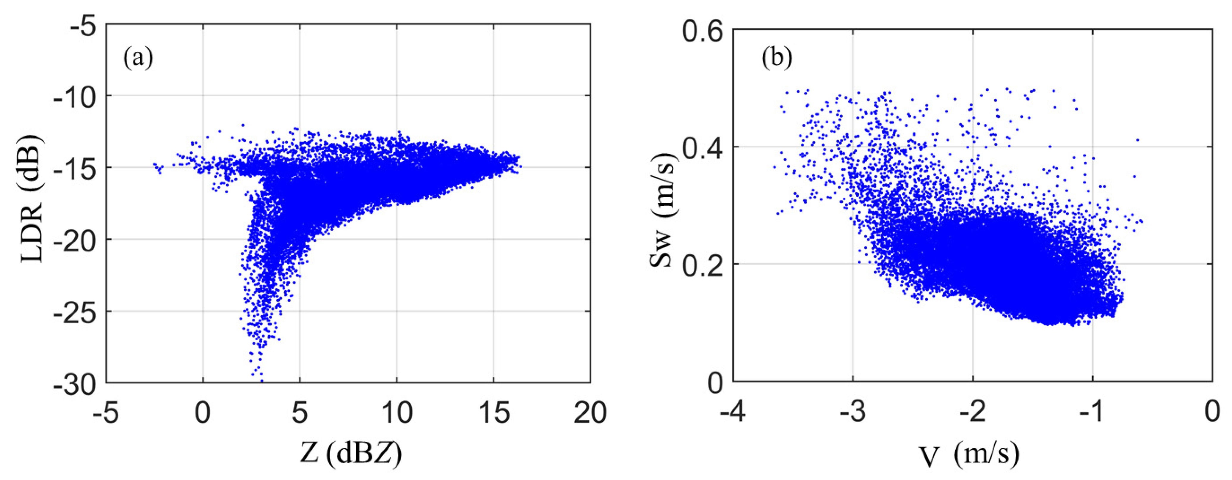
3.4. Description of Hydrometeor Classification Parameters

In all of the 42 winter precipitation cases, snow was observed each time, graupel was observed 13 times, and the mixture of snow and graupel was observed 20 times (

Table 2. 2016–2020 statistics based on observations of near-surface hydrometeor particles.

Year	Number of Cases
	Winter Precipitation	Snow	Graupel	Mixture of Snow and Graupel
2016	8	8	2	3
2017	5	5	2	2
2018	6	6	1	2
2019	15	15	5	8
2020	8	8	3	2
Total	42	42	13	20

). The XPOL and MMCR parameter ranges corresponding to different phases of hydrometeor particles are clarified based on both the parameter ranges in [1,9,21,34,35] and the observed 42 snowfall cases. Due to limited reliable data, the ranges of radar parameters corresponding to the phase of hydrometeor particles in the upper air layer are determined from relevant studies [21,35]. If the graupel is observed on the ground (Figure 7), the same method is used for the range of radar parameters (

Table 3. Ranges of XPOL and MMCR parameters and auxiliary temperature feature from microwave radiometer under different hydrometeor particle phases.

Hydrometeor	MMCR				XPOL			Microwave Radiometer
	Z (dBZ)	LDR (dB)	V (m/s)	Sw (m/s)	ZDR (dB)	KDP (°/km)	ρHV	T (°C)
Snow	−5~15	−22~−16	−2.5~0.5	0~0.6	−4.8~0.8	−0.1~1.2	0.66~0.99	−40~0
Ice	−40~0	−30~−18	−1.5~2	0~0.4	−2.25~1.5	0.09~1	0.4~0.9	−50~−10
Snow + Graupel	−20~15	−23~−14	−4.5~1	0.1~1	−2.5~2.5	−0.2~1.6	0.6~0.98	−40~5
Mixed	−25~10	−18~−11	−2~1	0.2~4	−0.8~1.5	0.1~1.2	0.6~0.9	−40~5
Liquid	−20~−10	−30~−20	−1~1	0.1~1	0~0.5	−0.06~0.26	0.97~1	−20~50
Graupel	2.5~16	−25~−13	−2.8~−1.2	0.1~0.5	−0.8~2.5	−0.2~1.6	0.91~0.96	−40~0

). It is also noted that the precipitation case on 29 November 2019 was used to verify the proposed hydrometeor classification method.

Four polarization parameters (i.e., $LDR$, $Z_{DR}$, $K_{DP}$ and ${\rho }_{HV}$) were used to classify the hydrometeor phases. In addition, temperature was considered as a key parameter in phase classification. The temperature profiles from microwave radiometer are consistent with those from the L-band digital radiosonde during the 30 snowfall cases (Figure 8). The average deviation is 3.2 °C and $\rho$ is 0.98, which are consistent with the result of [36].

4. Validation of Hydrometeor Classification at the Surface

Due to the scarcity of aircraft data, only the hydrometeor classification results near the surface have been validated, and the identification results of upper-air particles are discussed. A multi-phase transformation precipitation process occurred from 20 to 21 November 2016. As shown in Figure 9a,c,e, there were around three layers in the vertical direction, including the ice crystal layer, mixed snow-graupel layer and snowflake layer (or graupel particle layer) from top to bottom. At 21:30 on 20 November 2016, the size of graupel particles at the surface was between 1 and 3 mm. At 04:00 on 21 November 2016, a mixed snow-graupel was observed, with the snowflake size of 2–4 mm. It was also consistent with the MMCR phase-identification results at the same period (Figure 9a–d). For another snowfall case on 21 February 2017, hexagonal platelets and six-branched snowflakes were mainly observed, with the snowflake size at 4–6 mm. It also compared well with the MMCR phase identification result (Figure 9e,f).

We found that the phase identification method based on single MMCR is generally acceptable. The reason is that the diameter of precipitation particles near the surface is relatively large, and it is not difficult to distinguish from MMCR. However, identification becomes more difficult as the size and shape of upper-air particles are similar. Thus, it is necessary to identify the upper-air particle phases with both XPOL and MMCR.

5. Classification Results Based on X-/Ka-Band Radars and Verifications in Multiple Ways

On 29 November 2019, a Yellow River cyclone process occurred and lead to a snowfall storm. Under the steering of the vorticity advection and cold/warm advection at the leading edge of the upper-level trough, the near-surface cyclone gradually strengthened and moved eastward and northward. Meanwhile, a surface cyclone developed with an eastward movement, and the main cloud system of the snowfall occurred on the cyclone’s foreside. From 08:00 on 29 November to 08:00 of the next day, the average rainfall in Beijing was 3.9 mm, the highest level was 13.7 mm, and the maximum snow depth reached 11 cm. At around 08:00 on 30 November, the high-altitude trough gradually moved eastward, and the mid-high levels in Beijing were controlled by the northwest-western airflow and the snowfall process tended to the end. In this case, for both XPOL and MMCR, the surface SPI and the aircraft are used for joint observation. Figure 10a–c show the $Z_{DR}$, $K_{DP}$ and ${\rho }_{HV}$ from XPOL, respectively. Figure 10d–f show the patterns of $Z$, $V$ and $LDR$ from MMCR, respectively. The identification by the single MMCR (Figure 11a) and combination of the XPOL and MMCR (Figure 11b) indicate that three layers (i.e., ice crystal, mixed snow-graupel, and snowflake) exist in the vertical direction from top to bottom.

5.1. Comparison with the Surface Observation

From 17:48 to 18:48, hexagonal platelets and six-branched snowflakes were mainly detected, which was consistent with the classification results of hydrometeor particles near the surface in Figure 11. The images from 18:15 to 18:21 in Figure 12 show that surface hydrometeor particles were mainly six-branched snowflakes, with few hexagonal platelets. Additionally, the process of supercooled liquid-water riming on the snowflakes could be identified (i.e., the red circle). The riming degree indicated a low level of supercooled liquid water in the near-surface layer. Scattered mixed-phase areas, identified near the height of 2 km during 18:15–18:21 in Figure 11, imply that there was a small amount of liquid water in this storm event, and Figure 8c shows abundant moisture.

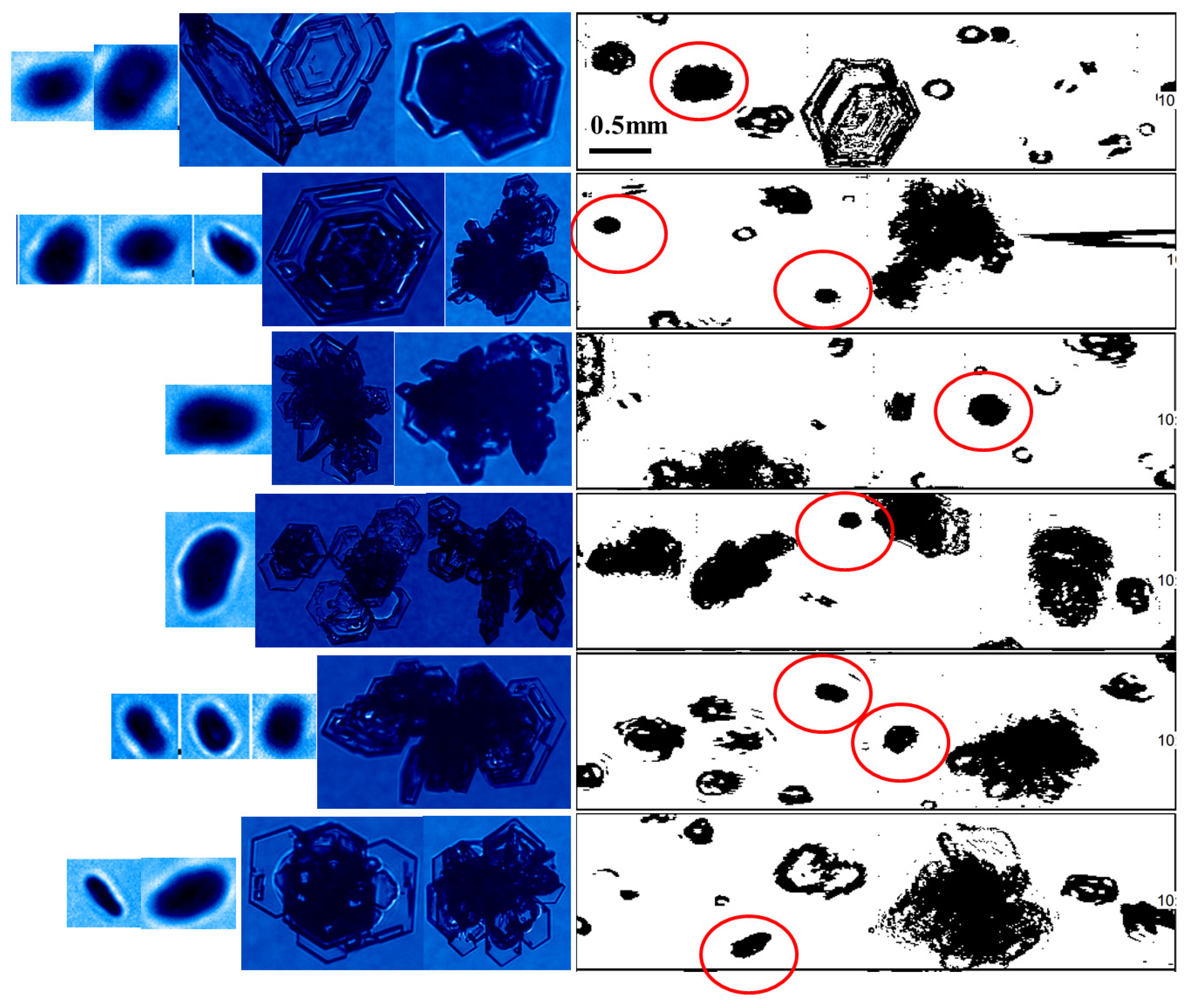
5.2. Comparison with the Aircraft Observation

From 18:18 to 19:30 on 29 November 2019, the King Air aircraft carried out joint detection with a radar in a spiral ascent for vertical detection over the cloud radar from 18:37 to 18:43. Due to air-traffic limitations, the effective detection range was 2263 m to 2563 m in the vertical direction. Figure 13 shows the flight path and vertical detection over the MMCR. Figure 14 shows the particle images observed by the aircraft from 18:37:50 to 18:42:06. The results show that the snow cloud system mainly consists of graupel particles (in the red circle), hexagonal platelets and six-branched snowflakes, with graupel particles of 0.2–0.5 mm. There was an aggregation among the hexagonal platelets and six-branched snowflakes in the upper air. Most of the snowflakes are larger than 1 mm. These results are consistent with the category of snow-graupel in Figure 11b, although inconsistent with the large range of graupel particles in Figure 11a. This indicates that the merged XPOL and MMCR results in higher accuracy than MMCR alone in identifying the phases of hydrometeor particles in the upper-air layer.

5.3. Compare with the WRF Simulations

Since numerous cloud microphysical schemes have been developed in numerical weather prediction models, the microphysical characteristics of the cloud system observed by radar and that simulated by the model have, recently, been mutually verified [37,38,39,40]. Weather Research and Forecasting (WRF) version 3.7 is used to simulate the snowfall process and to compare the phase identification by XPOL and MMCR. The application of the numerical model is a useful supplement to identify hydrometeor classification results.

The initial field and lateral boundary conditions are provided by the forecast field from the rapid-refresh multi-scale analysis and prediction system short term (RMAPS-ST). RMAPS-ST is a WRF-based regional numerical weather prediction (NWP) system, developed by the Institute of Urban Meteorology of Beijing Meteorological Service (IUM/BMS). It employs 9- and 3 km one-way nested domains, covering China and northern China. The conventional data (radiosonde, surface and aircraft reports) received by the Global Telecommunication System (GTS) includes data from automatic weather stations and radar observations in RMAPS-ST [41]. In this paper, the simulation adopts single-layer nesting, centered in Beijing with a horizontal resolution of 3 km and 300 × 300 grids. The model physics include the Yonsei University (YSU) planetary boundary layer (PBL) scheme [42], the unified Noah land surface model [43], the Rapid Radiative Transfer Model (RRTM) shortwave radiation [44], the New Goddard longwave radiation [45] and no cumulus scheme was adapted. The simulation began at 08:00 on 29 November and ended at 08:00 on 30 November 2019, where the first 6 h were used as a spin-up period and the output interval was 6 min. The cloud microphysics scheme adopted the Morrison scheme [46], which includes the prediction of the specific water content of cloud water, ice crystals, rain, snow, and graupel. The WRF mode and Morrison scheme are commonly used in the snowfall simulations [38,47]. In addition, these settings are often used in the simulation of convective systems and heavy precipitation events in China [48,49,50,51].

The evolutions of the MMCR observation and simulated radar echoes of the winter precipitation cloud system at the YJP station are shown in Figure 15. The characteristics of simulated radar echoes are similar to the MMCR observation. The height of radar echo is generally below 4 km, with an intensity of between 10 dBZ and 20 dBZ. Additionally, two snowfall events were clearly captured on the night of 29 November 2019, but the simulated radar echo intensity was found to be 5 dBZ stronger than the MMCR result.

The configuration and time-height evolution for the specific mass of snow, ice crystal and graupel simulated at the YJP station are demonstrated in Figure 16. The snowfall appears to have been below 3.5 km, and the maximum specific mass of snow was greater than 0.16 g/kg. In addition, ice crystal particles occurred at the height of 2–5 km in the middle and upper levels, with the maximum specific mass greater than 0.003 g/kg. A seeder-feeder effect was found in the precipitation cloud system since fine configuration was found between the large-value areas of ice crystal and snow in terms of time and height at upper and lower levels. Moreover, the graupel content was found to be small, due to limited supercooled cloud water. Overall, the locations of the simulated snowflakes, ice crystals and graupel are consistent with the phases of hydrometeor particles between XPOL and MMCR.

6. Summary

In this study, the hydrometeor characteristics of winter precipitation in northern China were investigated in 42 snowfall cases from 2016 to 2020, based on the multi-platform radar observation system, including ground-based (XPOL, MMCR, microwave radiometer, SPI, etc.) and airborne instruments. The particle-phase identification algorithm was established using both XPOL and MMCR under the fuzzy logic framework. The simulated hydrometeor results were verified with the ground-based radar observation network and were also compared with WRF simulations. The primary findings are as follows:

(1)

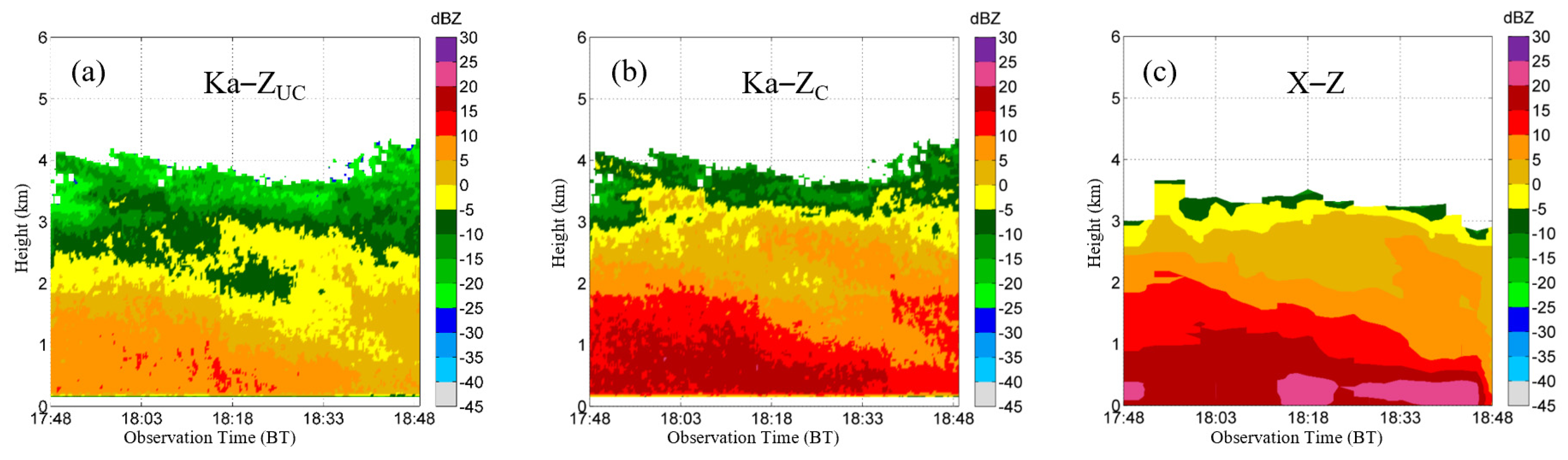
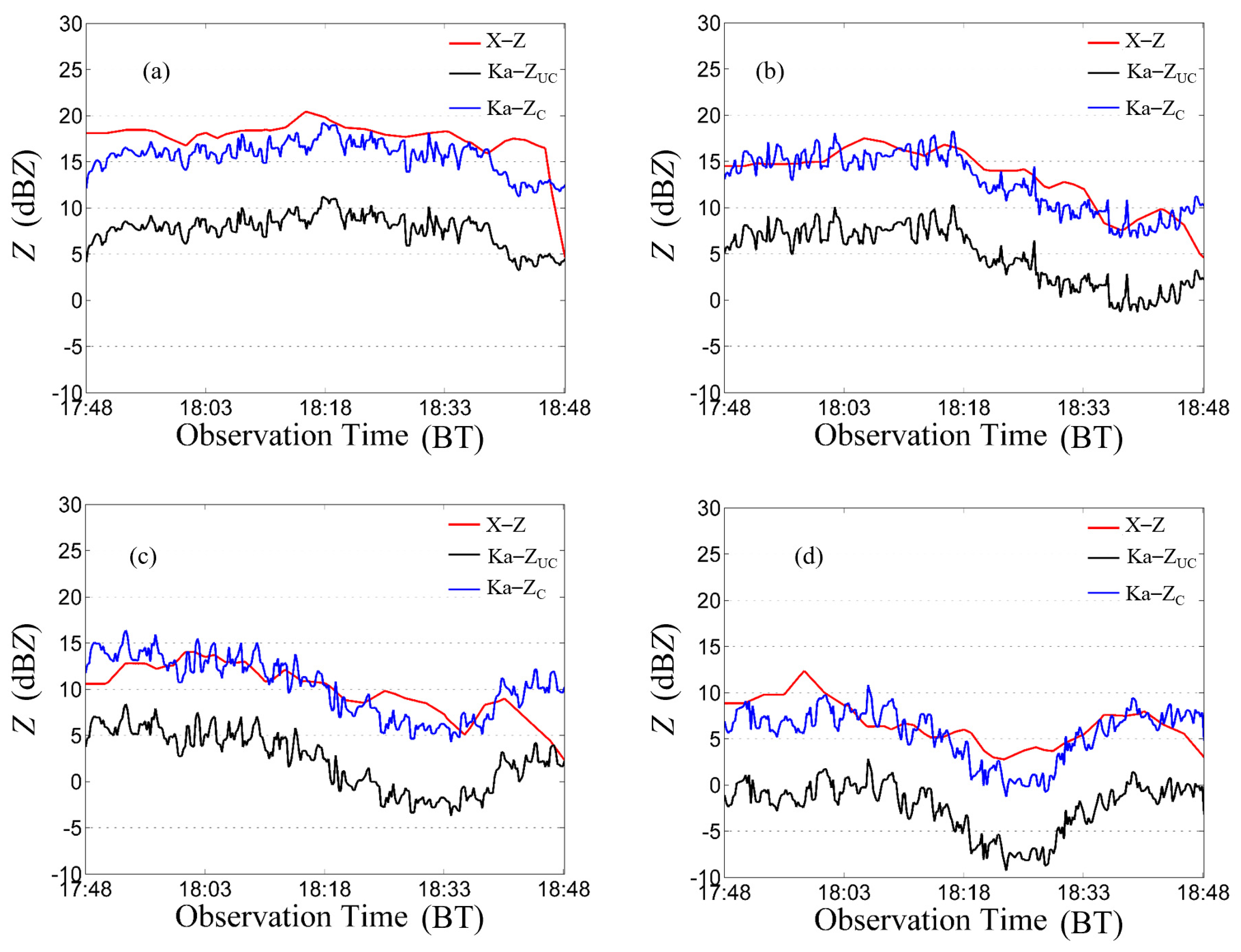
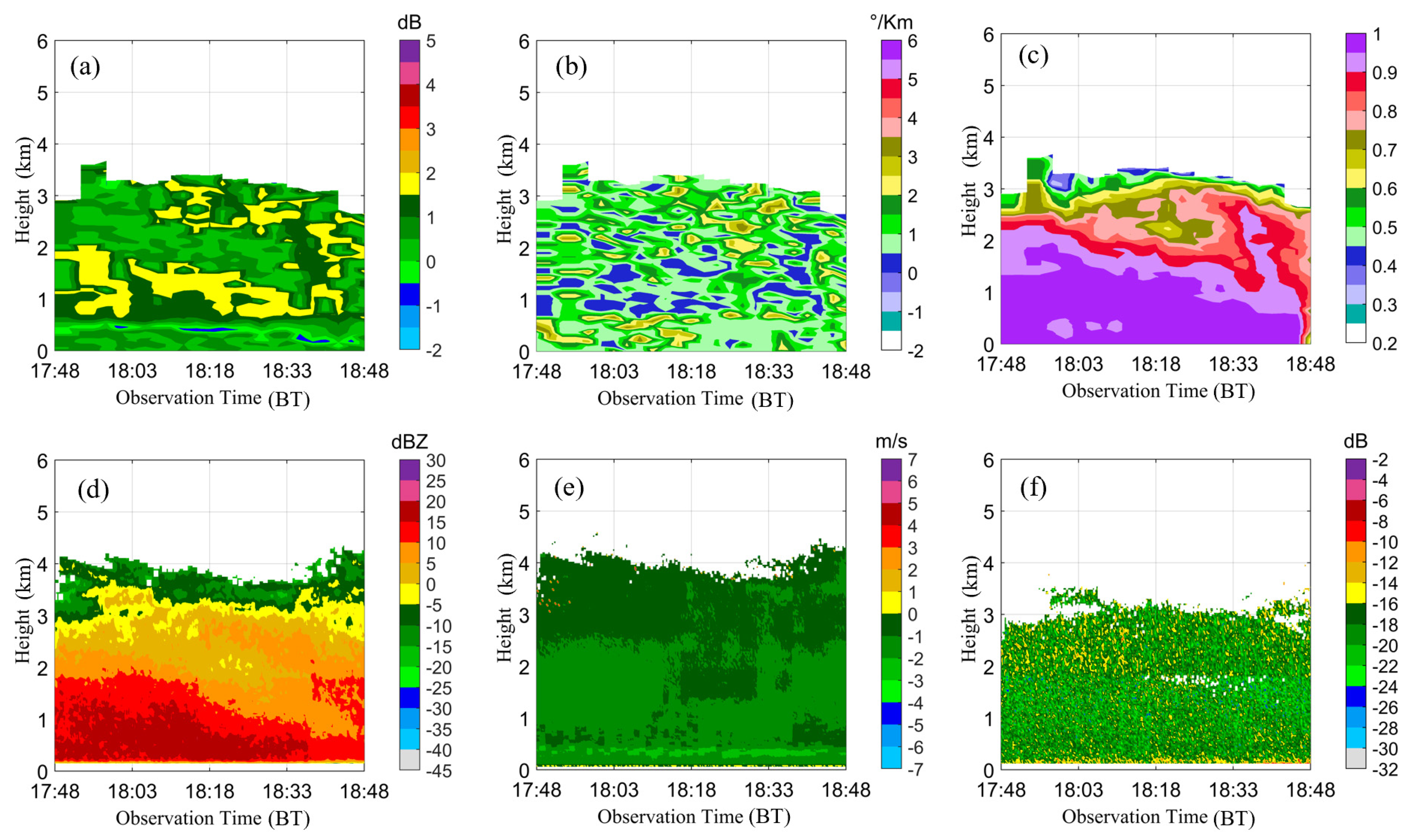
The MMCR reflectivity attenuation mainly derives from system deviation and snow on the antenna, whereby the attenuation is up to 8 dBZ. The corrected MMCR reflectivity is consistent with that in the XPOL, especially above the height of 1 km.

(2)

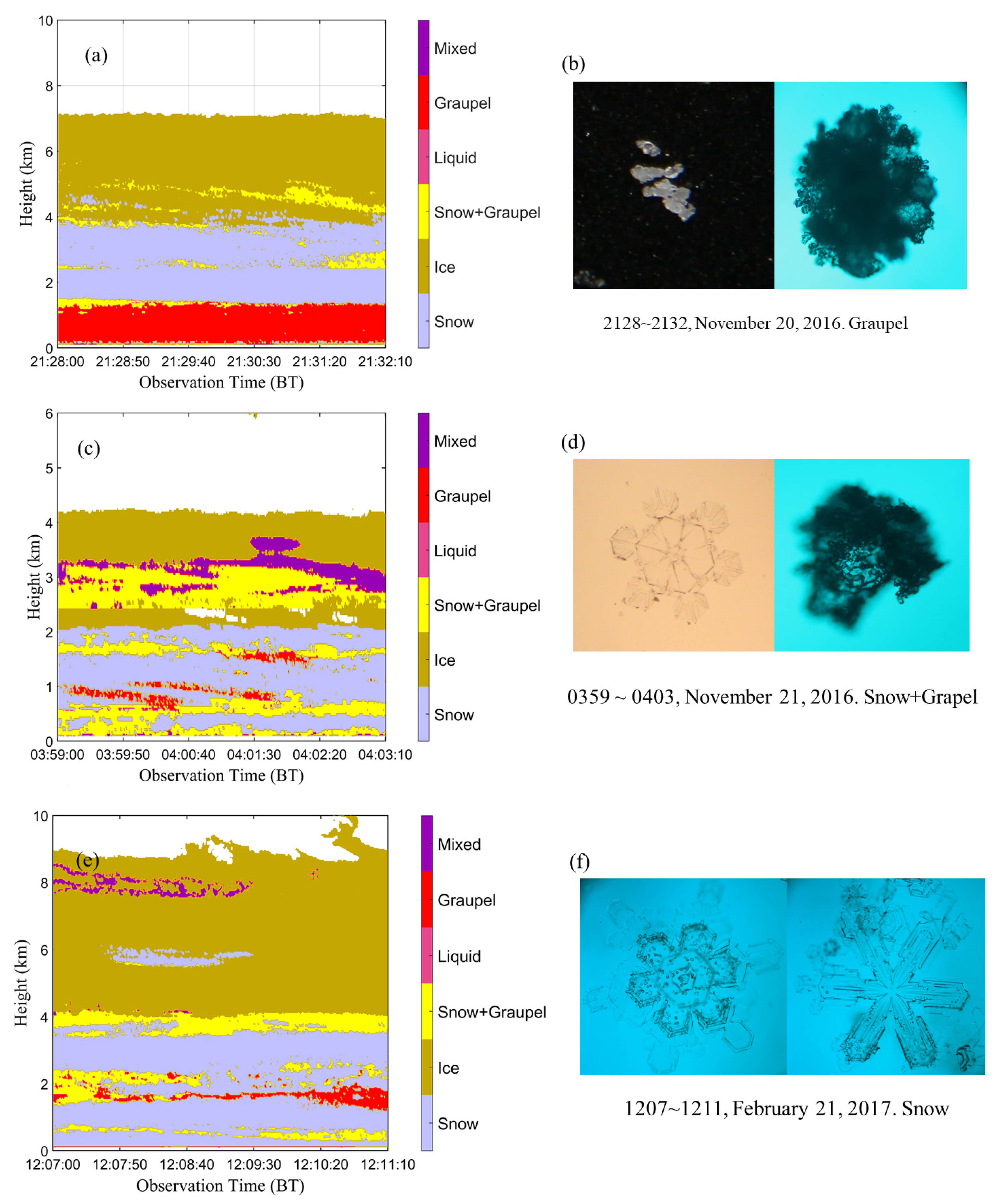
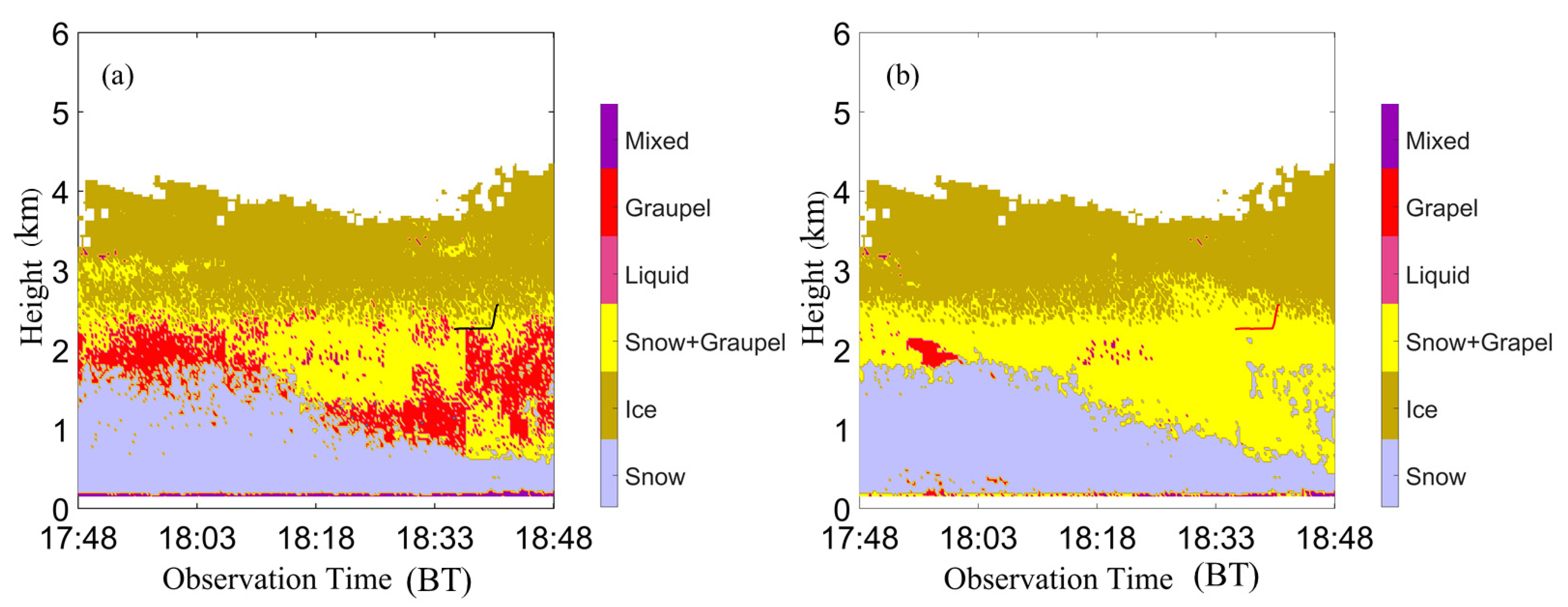
The ranges of XPOL and MMCR parameters were classified into three categories of particles (i.e., snow, graupel and mixture of snow and graupel). The hydrometeor classification result, identified by the MMCR, is highly consistent with the ground observations.

(3)

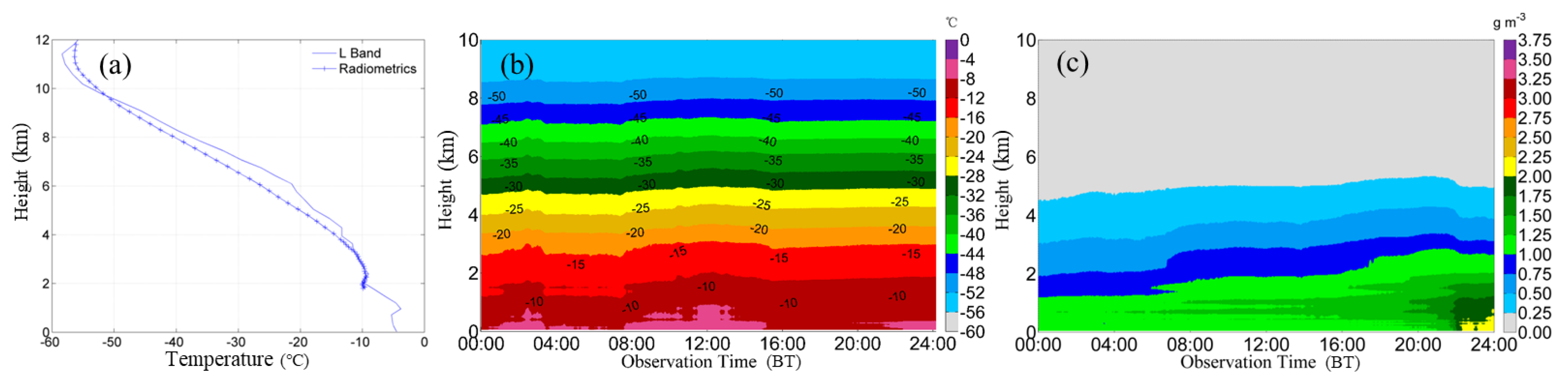
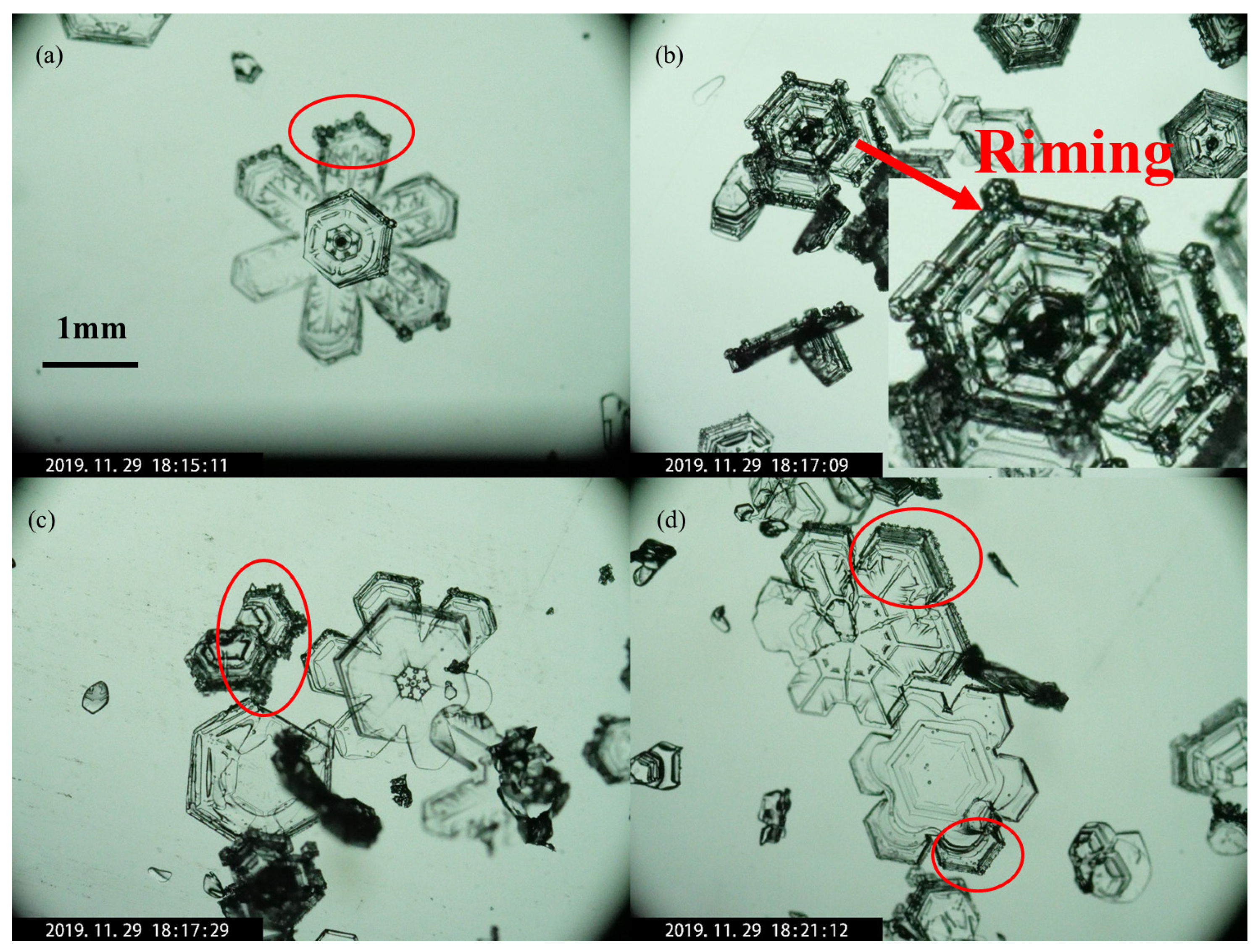
Three vertical layers, i.e., ice crystal, mixed snow–graupel and snowflake, exist from top to bottom in the winter precipitation cloud system. However, mixed-phases of snow and graupel exist in the upper air. In addition, the riming processes of various types of snowflakes were observed in the near-surface. This indicates that there was a small amount of supercooled liquid water found in the bottom.

(4)

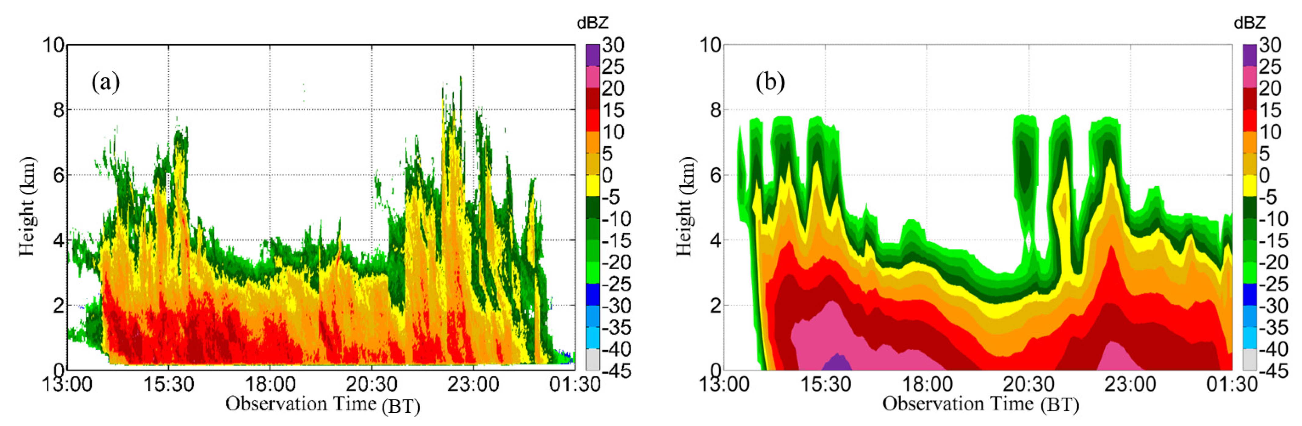
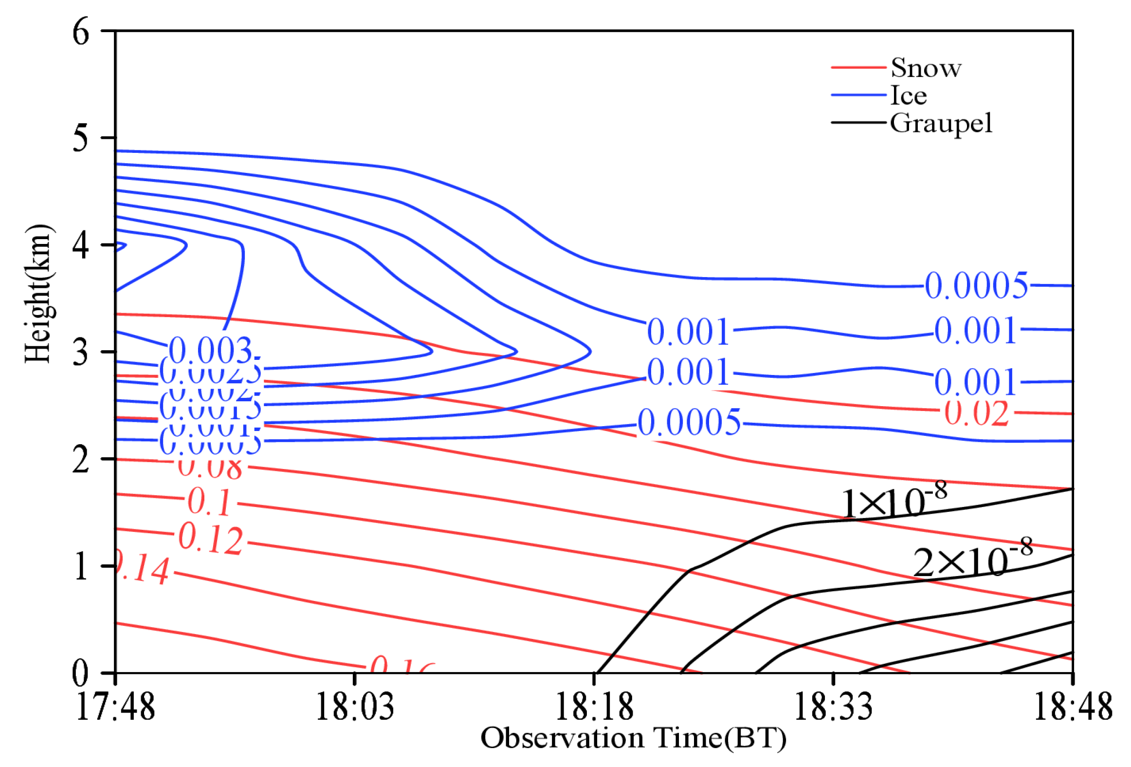
The simulated snowfall echo is similar to the MMCR result in terms of the evolution, echo intensity and echo top height. Moreover, the simulated position and specific mass of snow, ice crystal and graupel compare well with the identification results based on the combination of XPOL and MMCR.

As the microphysical process and phase variation of hydrometeor particles in the winter precipitation cloud system are complex, several important issues need to be discussed for the proposed hydrometeor classification algorithm, which include methods by which to set the weight coefficient of each parameter, how to best examine the accuracy of results with different weight coefficients, the representativeness of many samples for each category of hydrometeor particles, how to use more aircraft and ground observations to improve the identification results, and where the largest uncertainties in the classification exist, etc. If the identification results are significantly inconsistent with the observations, decisions on whether the radar parameter ranges corresponding to where two particles overlap with each other should be reconsidered. Afterwards, the size of the overlapped range needs to be considered to review whether it is necessary for the parameter range to be adjusted or the slope of β function to be adjusted. Furthermore, there are some clear uncertainties for the mixture of snow and graupel particles. For example, the proportion of graupel is critical, where few graupel might be identified as snow, and more graupel might be identified as graupel. Next, we will focus on the impact of the ratio of graupel on the recognition result. More specifically, additional winter precipitation studies are required to improve the proposed algorithm validation. Additionally, a more accurate identification of hydrometeor particles, based on the radar observations, is needed so as to validate and improve the precipitation cloud microphysical schemes.

References

1. Kennedy, P.C.; Rutledge, S.A. S-band dual-polarization radar observations of winter storms. J. Appl. Meteor. Climatol. 2011, 50, 844–858. [Google Scholar] [CrossRef]
2. Andrić, J.; Kumjian, M.R.; Zrnić, D.S.; Straka, J.M.; Melnikov, V.M. Polarimetric signatures above the melting layer in winter storms: An observational and modeling study. J. Appl. Meteor. Climatol. 2013, 52, 682–700. [Google Scholar] [CrossRef]
3. Bechini, R.; Baldini, L.; Chandrasekar, V. Polarimetric radar observations in the ice region of precipitating clouds at C-band and X-band radar frequencies. J. Appl. Meteor. Climatol. 2013, 52, 1147–1169. [Google Scholar] [CrossRef]
4. Wolde, M.; Vali, G. Polarimetric signatures from ice crystals observed at 95 GHz in winter clouds. Part I: Dependence on crystal form. J. Atmos. Sci. 2001, 58, 828–841. [Google Scholar] [CrossRef]
5. Vivekanandan, J.; Bringi, V.N.; Hagen, M.; Meischner, P. Polarimetric radar studies of atmospheric ice particles. IEEE Trans. Geosci. Remote Sens. 1994, 32, 1–10. [Google Scholar] [CrossRef] [Green Version]
6. Ryzhkov, A.V.; Zrnić, D.S.; Gordon, B.A. Polarimetric method for ice water content determination. J. Appl. Meteor. 1998, 37, 125–134. [Google Scholar] [CrossRef]
7. Kumjian, M.R.; Ryzhkov, A.V.; Reeves, H.D.; Schuur, T.J. A dual-polarization radar signature of hydrometeor refreezing in winter storms. J. Appl. Meteor. Climatol. 2013, 52, 2549–2566. [Google Scholar] [CrossRef]
8. Bringi, V.N.; Chandrasekar, V. Polarimetric Doppler Weather Radar: Principles and Applications; Cambridge University Press: Cambridge, UK, 2001; p. 636. [Google Scholar]
9. Straka, J.K.; Zrnić, D.S. An algorithm to deduce hydrometeor types and contents from multi-parameter radar data. Preprints, 26th Conf. on Radar Meteorology, Norman, OK. Am. Meteor. Soc. 1993, 513, 516. [Google Scholar]
10. Holler, H.; Bringi, V.N.; Hagen, M.; Meischner, P.F. Life cycle and precipitation formation in a hybrid-type hailstorm revealed by polarimetric and doppler radar measurements. J. Atmos. Sci. 1994, 51, 2500–2522. [Google Scholar] [CrossRef]
11. Liu, H.; Chandrasekar, V. Classification of hydrometeors based on polarimetric Radar measurements: Development of fuzzy logic and neuro-fuzzy systems and in-situ verification. J. Atmos. Ocean. Technol. 2000, 17, 140–164. [Google Scholar] [CrossRef]
12. Zeng, Z.X.; Sandra, E.Y.; Robert, A.H.; David, E.K. Microphysics of the Rapid Development of Heavy Convective Precipitation. Mon. Weather Rev. 2001, 129, 1882–1904. [Google Scholar] [CrossRef] [Green Version]
13. Ryzhkov, A.V.; Schuur, T.J.; Burgess, D.W.; Heinselman, P.L.; Giangrande, S.E.; Zrnić, D.S. The Joint Polarization Experiment: Polarimetric rainfall measurements and hydrometeor classification. Bull. Am. Meteor. Soc. 2005, 86, 809–824. [Google Scholar] [CrossRef] [Green Version]
14. Heinselman, P.L.; Ryzhkov, A.V. Validation of polarimetric hail detection. Weather Forecast. 2006, 21, 839–850. [Google Scholar] [CrossRef]
15. Park, H.S.; Ryzhkov, A.V.; Zrnić, D.S.; Kim, K.-E. The hydrometeor classification algorithm for the polarimetric WSR-88D: Description and application to an MCS. Weather Forecast. 2009, 24, 730–748. [Google Scholar] [CrossRef]
16. Apffel, K.R.; Reynolds, A.; Zaff, D. Improving the Quantitative Precipitation Estimate for Hydrometeors Classified as Dry Snow by Polarimetric Radars. NOAA/National Weather Service Eastern Regional Tech. Attachment. 2015; p. 6. Available online: https://www.weather.gov/media/erh/ta2015-06.pdf (accessed on 4 December 2021).
17. Kurdzo, J.M.; Bennett, B.J.; Smalley, D.J.; Donovan, M.F. The WSR-88D Inanimate Hydrometeor Class. J. Appl. Meteor. Climatol. 2020, 59, 841–858. [Google Scholar] [CrossRef] [Green Version]
18. Elmore, K.L. The NSSL hydrometeor classification algorithm in winter surface precipitation: Evaluation and future development. Weather Forecast. 2011, 26, 756–765. [Google Scholar] [CrossRef]
19. Thompson, E.J.; Rutledge, S.A.; Dolan, B.; Chandrasekar, V.; Cheong, B.L. A dual-polarization radar hydrometeor classification algorithm for winter precipitation. J. Atmos. Ocean. Technol. 2014, 31, 1457–1481. [Google Scholar] [CrossRef] [Green Version]
20. Reinking, R.F.; Matrosov, S.Y.; Bruintjes, R.T.; Martner, B.E. Identification of hydrometeors with elliptical and linear polarization Ka-band radar. J. Appl. Meteor. 1997, 36, 322–339. [Google Scholar] [CrossRef]
21. Shupe, M.D. A ground-based multiple remote-sensor cloud phase classifier. Geophys. Res. Lett. 2007, 34, L22809. [Google Scholar] [CrossRef] [Green Version]
22. Khain, A.P.; Pinsky, M.; Magaritz, L.; Krasnov, O.; Russchenberg, H.W. Combined observational and model investigations of the Z-LWC 216 relationship in strato-cumulus clouds. J. Appl. Met. Clim. 2008, 47, 591–606. [Google Scholar] [CrossRef]
23. Mace, G.G.; Heymsfield, A.J.; Poellot, M.R. On retrieving the microphysical properties of cirrus clouds using the moments of the millimeter-wavelength Doppler spectrum. J. Geophys. Res. 2002, 107, 4815. [Google Scholar] [CrossRef] [Green Version]
24. Liu, L.P.; Zheng, J.F.; Ruan, Z. The preliminary analyses of the cloud properties over the Tibetan Plateau from the field experiments in clouds precipitation with the vavious radars. Acta Meteorol. Sin. 2015, 73, 635–647. [Google Scholar]
25. Chen, Y.C.; Jin, Y.L.; Ding, D.P. Preliminary analysis on the application of millimeter wave cloud radar on snow observation. J. Atmos. Sci. 2018, 42, 134–149. (In Chinese) [Google Scholar]
26. Li, H.; Korolev, A.; Moisseev, D. Supercooled liquid water and secondary ice production in Kelvin–Helmholtz instability as revealed by radar Doppler spectra observations. Atmos. Chem. Phys. 2021, 21, 13593–13608. [Google Scholar] [CrossRef]
27. Li, H.; Moisseev, D. Two layers of melting ice particles within a single radar bright band: Interpretation and implications. Geophys. Res. Lett. 2020, 47, e2020GL087499. [Google Scholar] [CrossRef]
28. Li, H.; Tiira, J.; von Lerber, A.; Moisseev, D. Towards the connection between snow microphysics and melting layer: Insights from multifrequency and dual-polarization radar observations during BAECC. Atmos. Chem. Phys. 2020, 20, 9547–9562. [Google Scholar] [CrossRef]
29. Li, Y.L.; Sun, X.J.; Zhao, S.J. Analysis of snowfall’s microphysical process from Doppler spectrum using Ka-band millimeter-wave cloud radar. J. Infrared. Millim. Waves 2019, 38, 245–253. [Google Scholar]
30. Matrosov, S.Y. Modeling backscatter properties of snowfall at millimeter wavelengths. J. Atmos. Sci. 2007, 64, 1727–1736. [Google Scholar] [CrossRef]
31. Matrosov, S.Y.; Shupe, M.D.; Djalalova, I.V. Snowfall Retrievals Using Millimeter-Wavelength Cloud Radars. J. Appl. Meteor. Climatol. 2008, 47, 769–777. [Google Scholar] [CrossRef] [Green Version]
32. Battan, L.J. Radar Observations of the Atmosphere; University of Chicago Press: Chicago, IL, USA, 1973; p. 324. [Google Scholar]
33. Matrosov, S.Y. A Dual-Wavelength Radar Method to Measure Snowfall Rate. J. Appl. Meteor. Climatol. 1998, 37, 1510–1521. [Google Scholar] [CrossRef]
34. He, Y.X.; Xiao, H.; Lü, D.R. Analysis of hydrometeor distribution characteristics in stratiform clouds using polarization radar. J. Atmos. Sci. 2010, 34, 23–34. (In Chinese) [Google Scholar]
35. Wang, D.W.; Liu, L.P.; Zong, R. Fuzzy Logic Method in Retrieval Atmospheric Cloud Particle Phases and Effect Analysis. Meteor. Mon. 2015, 41, 171–181. [Google Scholar]
36. Han, J.J.; Chen, F.; Zhang, Z. Assessment and Characteristics of MP-3000A Ground-Based Microwave Radiometer. Meteor. Mon. 2015, 41, 226–233. [Google Scholar]
37. Liu, X.E.; He, H.; Gao, Q. Research on application of the mesoscale silver iodide seeding numerical model. Acta Meteor. Sin. 2021, 79, 359–368. [Google Scholar]
38. Han, M.; Braun, S.A.; Matsui, T.; Williams, C.R. Evaluation of cloud microphysics schemes in simulations of a winter storm using radar and radiometer measurements. J. Geophys. Res. Atmos. 2013, 118, 1401–1419. [Google Scholar] [CrossRef]
39. Takamichi, I.; Toshihisa, M. Advances in Clouds and Precipitation Modeling Supported by Remote Sensing Measurements. In Remote Sensing of Clouds and Precipitation; Springer International Publishing: New York, NY, USA, 2018; pp. 257–277. [Google Scholar]
40. Gang, C.; Kun, Z.; Hao, H.; Zheng, W.Y.; Ying, H.L.; Ji, Y. Evaluating Simulated Raindrop Size Distributions and Ice Microphysical Processes with Polarimetric Radar Observations in a Meiyu Front Event Over Eastern China. J. Geophys. Res. Atmos. 2021, 126, 22. [Google Scholar]
41. Zhong, J.; Lu, B.; Wang, W.; Huang, C.; Yang, Y. Impact of Soil Moisture on Winter 2-m Temperature Forecasts in Northern China. J. Hydrometeor. 2020, 21, 597–614. [Google Scholar] [CrossRef]
42. Hong, S.-Y.; Noh, Y.; Dudhia, J. A new vertical diffusion package with an explicit treatment of entrainment processes. Mon. Weather Rev. 2006, 134, 2318–2341. [Google Scholar] [CrossRef] [Green Version]
43. Chen, F.; Dudhia, J. Coupling an advanced land surface–hydrology model with the Penn State–NCAR MM5 modeling system. Part I: Model implementation and sensitivity. Mon. Weather Rev. 2001, 129, 569–585. [Google Scholar] [CrossRef] [Green Version]
44. Mlawer, E.J.; Taubman, S.J.; Brown, P.D.; Iacono, M.J.; Clough, S.A. Radiative transfer for inhomogeneous atmospheres: RRTM, a validated correlated-k model for the longwave. J. Geophys. Res. 1997, 102, 16663–16682. [Google Scholar] [CrossRef] [Green Version]
45. Chou, M.; Suarez, M. A solar radiation parameterization (CLIRAD-SW) for atmospheric studies. NASA Tech. Memo. 1999, 40, 104606. [Google Scholar]
46. Morrison, H.; Curry, J.; Khvorostyanov, V. A new double-moment microphysics parameterization for application in cloud and climate models. Part I: Description. J. Atmos. Sci. 2005, 62, 1665–1677. [Google Scholar] [CrossRef]
47. Molthan, A.; Colle, B. Comparisons of single and double moment microphysics schemes in the simulation of a synoptic-scale snowfall event. Mon. Weather Rev. 2012, 140, 29823002. [Google Scholar] [CrossRef]
48. Qian, Q.; Lin, Y.; Luo, Y.; Zhao, X.; Zhao, Z.; Luo, Y.; Liu, X. Sensitivity of a simulated squall line during Southern China Monsoon Rainfall Experiment to parameterization of microphysics. J. Geophys. Res. Atmos. 2018, 123, 4197–4220. [Google Scholar] [CrossRef]
49. Zhang, S.; Parsons, D.B.; Xu, X.; Wang, Y.; Liu, J.; Abulikemu, A.; Shen, W.; Zhang, X.; Zhang, X. A modeling study of an atmospheric bore associated with a nocturnal convective system over China. J. Geophys. Res. Atmos. 2020, 125, e2019JD032279. [Google Scholar] [CrossRef]
50. Yang, Q.; Yu, Z.; Wei, J.; Yang, C.; Kunstmann, H. Performance of the WRF Model in Simulating Intense Precipitation Events over the Hanjiang River Basin, China—A Multi-Physics Ensemble Approach. Atmos. Res. 2020, 248, 105206. [Google Scholar] [CrossRef]
51. Yuan, F.; Heng, C.L.; Jie, F.Y.; Zhi, B.G. Evaluating the performance of a WRF microphysics ensemble through comparisons with aircraft observations. Atmos. Ocean. Sci. Lett. 2021, 14, 100013. [Google Scholar]
Figure 1. Information of the multi-platform radar observation system: (a) Topographic map around the YJP station and aircraft track projection, (b) Photo of surface observation network, (c) XPOL radar and (d) Kingair aircraft. The Chinese in the figure is the company name.
Remotesensing 13 05070 g001
Figure 2. Comparison between estimated snowfall (red line: original Z , black line: corrected Z ) and observed snowfall by weighing gauges (blue line) for (a) hourly and (b) accumulation, respectively, on 29 November 2019 from 14:00 to 02:00 the next day.
Remotesensing 13 05070 g002
Figure 3. The XPOL and MMCR reflectivity within 17:48–18:48 on 29 November 2019 (a) before the MMCR reflectivity correction and (b) after the MMCR reflectivity correction, (c) XPOL reflectivity.
Remotesensing 13 05070 g003
Figure 4. Comparison between XPOL and MMCR reflectivity at different heights, i.e., (a) 500 m, (b) 1000 m, (c) 1500 m, and (d) 2000 m, from 17:48 to 18:48 on 29 November 2019.
Remotesensing 13 05070 g004
Figure 5. A fuzzy system for hydrometeor type classification.
Remotesensing 13 05070 g005
Figure 6. The β function graphs of Z corresponding to different hydrometeor particles.
Remotesensing 13 05070 g006
Figure 7. Scatter diagram of the relationships among the MMCR parameters in surface graupel processes: (a) Z-LDR and (b) V-Sw.
Remotesensing 13 05070 g007
Figure 8. (a) Comparison of temperature profiles between radiosonde and microwave radiometer at the 30 snowfall events, (b) temperature, (c) water vapor from microwave radiometer on 29 November 2019.
Remotesensing 13 05070 g008
Figure 9. Phase classifications for hydrometeor particles (a,c,e) identified by the single MMCR and (b,d,f) observed in the near-surface in corresponding periods.
Remotesensing 13 05070 g009
Figure 10. XPOL and MMCR parameters of the snowfall cloud system from 17:48 to 18:48 on 29 November 2019. (ac): XPOL ( Z D R , K D P and ρ H V ), respectively, and (df): MMCR ( Z , V and L D R ), respectively.
Remotesensing 13 05070 g010
Figure 11. Phase classifications for hydrometeor particles from 17:48 to 18:48 on 29 November 2019 based on (a) MMCR (18:37–18:42, the black line at the height of 2.2–2.5 km is the aircraft detection area) and (b) combination of XPOL and MMCR (the red line: same as the black line in (a)).
Remotesensing 13 05070 g011
Figure 12. (ad) Images of surface hydrometeor particles from 18:15 to 18:21 on 29 November 2019.
Remotesensing 13 05070 g012
Figure 13. Flight path (red line is the vertical detection area above the cloud radar).
Remotesensing 13 05070 g013
Figure 14. Particle images observed by the aircraft (graupel particles are in the red circle) from 18:37:50 to 18:42:06.
Remotesensing 13 05070 g014
Figure 15. Time-height evolutions of (a) MMCR and (b) simulated radar echoes.
Remotesensing 13 05070 g015
Figure 16. Simulated configuration and time-height evolution for the specific mass of snow, ice crystal and graupel at YJP station.
Remotesensing 13 05070 g016