
Review of Image Classification Algorithms Based on Convolutional Neural Networks


Abstract
: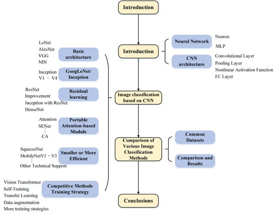
1. Introduction
2. Overview of CNNs
2.1. Neural Network
2.1.1. Neuron
2.1.2. Multilayer Perceptron (MLP)
2.2. CNN Architecture
2.2.1. Convolutional Layer
2.2.2. Pooling Layer
2.2.3. Nonlinear Activation Function
2.2.4. Fully Connected (FC) Layer
2.2.5. Loss Function
2.2.6. Optimizer
3. Image Classification Based on CNN
3.1. Classic CNN Models
3.1.1. LeNet Network
3.1.2. AlexNet Network
- ReLU [73]. The activation function is changed from sigmoid to ReLU, it accelerates the model convergence and reduces the gradient disappearance.
- Dropout [79]. the model uses dropout to control the model complexity of the fully connected layer with to alleviate the overfitting problem.
- Data augmentation. Introduced a large number of Data augmentation, such as flipping, cropping, and color changes, to further enlarge the datasets to alleviate the overfitting problem. Dropout and Data augmentation methods are widely used in subsequent convolutional neural networks.
- Overlapping pooling. There will be overlapping areas between adjacent pooling windows, which can improve model accuracy and alleviate overfitting.
3.1.3. VGGNet
- Modular network. VGGNet uses a lot of basic modules to construct the model, this idea has become the construction method of DCNNs.
- Smaller convolution. A lot of 3 × 3 convolution filters are used on VGGNet, which can ensure that the depth of the network is increased, and the model parameters are reduced under the same receptive field compared with a larger convolution filter [102].
- Multi-Scale training. It first scales the input image to a different size , and then randomly crops it to a fixed size of 224 × 224 and trains the obtained data of multiple windows together. This process is regarded as a kind of scale jitter processing, which can achieve the effect of data augmentation and prevent the model from overfitting [102].
3.1.4. Network in Network (NIN)
- Mlpconv. MLP layer is equivalent to a 1 × 1 convolutional layer. Now, it is usually used to adjust the channels and the parameters, and there are also explanations that cross-channel interaction and information integration are possible.
- Global average pooling (GAP). The FC layer is no longer used for output classification, but a micro-network block with the number of output channels equal to the number of label categories is used, and then all elements in each channel are averaged through a GAP layer to obtain the classification confidence.
3.2. GoogLeNet/InceptionV1 to V4
3.2.1. InceptionV1
- Inception module. Although the early traditional neural networks used random sparse connections, computer hardware was inefficient in computing non-uniform sparse connections. The proposed Inception module can not only maintain the sparsity of the network structure but also use the high computational performance of the dense matrix, thereby effectively improving the model’s utilization of parameters.
- GAP. Replaced the fully connected layer to reduce the parameters.
- Auxiliary classifier. An auxiliary classifier used for a deeper network is a small CNN inserted between layers during training, and the loss incurred is added to the main network loss.
3.2.2. InceptionV2
- (1)
- Smaller convolution. The 5 × 5 convolution is replaced by the two 3 × 3 convolutions. This also decreases computational time and thus increases computational speed because a 5 × 5 convolution is 2.78 more expensive than a 3 × 3 convolution.
- (2)
- Batch Normalization (BN). BN is a method used to make ANNs faster and more stable through normalization of the layers’ inputs by re-centering and re-scaling for each mini-batch.
- /mini-batch mean:
- /mini-batch variance:
- /normalize:
- /scale and shift:
3.2.3. InceptionV3
- Factorized convolutions. This helps to reduce the computational efficiency as it reduces the number of parameters involved in a network. It also keeps a check on the network efficiency. This part contains the following (2) and (3).
- Smaller convolutions. replacing bigger convolutions with smaller convolutions definitely leads to faster training.
- Asymmetric convolutions. A 3 × 3 convolution could be replaced by a 1 × 3 convolution followed by a 3 × 1 convolution. The number of parameters is reduced by 33%.
- Grid size reduction. Grid size reduction is usually done by pooling operations. However, to combat the bottlenecks of computational cost, a more efficient technique is proposed. Say for example in the Figure 12, 320 feature maps are done by conv with stride 2. 320 feature maps are obtained by max pooling. And these 2 sets of feature maps are concatenated as 640 feature maps and go to the next level of inception module.
3.2.4. InceptionV4
- The initial set of layers to which the paper refers “stem of the architecture” (Figure 14) was modified to make it more uniform. These layers are used before the Inception block in the architecture.
- This model can be trained without partition of replicas unlike the previous versions of inceptions which required different replicas to fit in memory. This architecture uses memory optimization on backpropagation to reduce the memory requirement.
3.3. Residual Learning Networks
3.3.1. ResNet
- This method is easy to optimize, but the “plain” networks (that simply stack layers) show higher training error when the depth increases.
- It can easily gain accuracy from greatly increased depth, producing results that are better than previous networks.
3.3.2. Improvement of ResNet
- ResNet with Pre-activation. He et al. [109] proposed a pre-activation structure to pre-activate the BN and ReLU to further improve the network performance. Several experiments were carried out on the layout of BN and ReLU and the best performing structure was obtained in Figure 17(right). It can successfully train ResNet with more than 1000 layers. At the same time, they also proved the importance of identity mapping compared to other shortcut connections.
- Stochastic depth. The authors of [117] pointed out that there are many layers in the ResNet network that contribute little to the output result. In the network training process, the Stochastic depth method is used, and deleting some layers can greatly shorten the training time and effectively increase the depth of ResNet, even exceeding 1200 layers. The test error and the training time on CIFAR-10/100 still has a good improvement.
- Wide Residual Networks (WRNs). With the increasing depth of residual networks, the diminishing feature reuse will make the training of the network very slow [118]. To alleviate this problem, ref. [119] introduced a wide-dropout block that widens the weight layer of the original residual unit [25] Figure 15 (right) and adds dropout between the two weight layers. Compared with deeper ResNet, WRN with fewer layers greatly reduces the training time and has better performance on the CIFAR&ImageNet data set.
- ResNeXt [26]. Although Inception and ResNet have great performance, but these models are well-suited for several datasets. Due to the many hyperparameters and computations involved, adapting them to new datasets is no minor task. A new dimension “Cardinality C”—the number of paths in a block—is used to overcome this problem, and experiments demonstrate that increasing cardinality C is more effective than going deeper or wider when we increase the capacity. The authors compared the completely equivalent structures of the three mathematical calculations in Figure 18. The experimental results show that block Figure 18c with grouped convolution is more succinct and faster than the other two forms, and ResNeXt uses this structure as a basic block.
- Dilated Residual Networks (DRN). To solve the decrease in the resolution of the feature map and the loss of feature information caused by downsampling. However, simply removing subsampling steps in the network will reduce the receptive field. So, Yu et al. [120] introduced dilated convolutions that are used to increase the receptive field of the higher layers and replaced a subset of the internal downsampling layer based on the residual network, compensating for the reduction in receptive field induced by removing subsampling. Compared to ResNet with the same parameter amount, the accuracy of DRN is significantly improved in image classification.
- Other models. Veit et al. [121] drops some of the layers of a trained ResNet and still have comparable performance. Resnet in Resnet (RiR) [122] proposed a deep dual-stream architecture that generalizes ResNets and standard CNNs and is easily implemented with no computational overhead. DropBlock [123] technique discards feature in a contiguous correlated area called block, which is a regularization helpful in avoiding the most common problem data science professionals face i.e., overfitting. Big Transfer (BiT) [124] proposes a general transfer learning method to be applied to ResNet, which uses the minimal number of tricks yet attains excellent performance on many tasks. NFNet [125] proposes a ResNet-based structure without BN layer, by using adaptive gradient clipping technique to achieve amazing training speed and accuracy.
3.3.3. ResNet with Inception
- Inception-ResNet [107]. Tried to combine the Inception structure with the residual structure and achieved good performance. It comes from the same paper as inceptionV4 [107], and the combination is Inception-ResNet-V1/V2 as shown in Figure 19 and Figure 20. Inception-ResNet-V1 has roughly the computational cost of Inception-V3 [1], and it was training much faster but reached slightly worse final accuracy than InceptionV3. Inception-ResNet-V2 has roughly the computational cost of Inception-v4, and it was training much faster and reached slightly better final accuracy than InceptionV4 [107].
- Xception [126]. It is based on the design point of InceptionV3 [1]. The author believes that the correlation between channels and spatial correlation should be handled separately, using modified depthwise separable [127] convolution to replace the convolution operation in InceptionV3. Refs. [128,129] also show that using separable convolution can reduce the size and computational cost of CNNs. But the modification in Xception aims to improve performance. The accuracy of Xception on ImageNet is slightly higher than that of Inception-v3, while the parameters is slightly reduced. The experiment in [126] also shows that the residual connection mechanism similar to ResNet added to Xception can significantly speed up the training times and obtain a higher accuracy rate.
- PolyNet [130]. Many studies tend to increase depth and width in image classification tasks to obtain higher performance. But very deep networks will have trouble that is a diminishing return and increased training difficulty. A quadratic growth in both computational cost and memory demand is caused by a widening network. This method explores the structural diversity of Inception and ResNet that a new dimension beyond just depth and width, which introduced a better-mixed model from the perspective of polynomials.
3.3.4. DenseNet
3.4. Attention Module for CNNs
3.4.1. Residual Attention Neural Network
- Stacking multi-attention modules has made RAN very effective at recognizing noisy, complex, and cluttered images.
- RAN’s hierarchical organization gives it the capability to adaptively allocate a weight for every feature map depending on its importance within the layers.
- Incorporating three distinct levels of attention (spatial, channel, and mixed) enables the model to use this ability to capture the object-aware features at these distinct levels.
3.4.2. SENet
3.4.3. BAM and CBAM
3.4.4. GENet
3.4.5. SKNet
3.4.6. GSoP-Net
3.4.7. ECA-Net
3.4.8. Coordinate Attention
3.4.9. Other Attention Modules and Summary
3.5. Smaller or More Efficient Network
3.5.1. SqueezeNet
3.5.2. MobileNet V1 to V3
3.5.3. ShuffleNet V1 to V2
3.5.4. PeleeNet
3.5.5. MnasNet
3.5.6. More Backbone Networks for Real-Time Vision Tasks
- CSPNet. Wu et al. [169] proposed Cross Stage Partial Network (CSPNet) to solve the problem of heavy inference computations, which is caused by the duplicate gradient information within network optimization. A large amount of gradient information in DenseNet [131] is reused for updating weights of different dense layers, which will result in different dense layers repeatedly learning copied gradient information. The network modifies the equations of the feed-forward pass and weight updating that the gradients coming from the dense layers are separately integrated and the feature map that did not go through the dense layers is also separately integrated. It preserves the advantages of DenseNet’s feature reuse characteristics but at the same time prevents an excessive amount of duplicate gradient information by truncating the gradient flow. It also designed partial transition layers is to maximize the difference of gradient combination. CSPNet can be easily applied to DenseNet [131], ResNet [25] and ResNeXt [26].
- VarGNet. In 2019, Variable Group Network (VarGNet) [170], by Zhang et al. makes a compromise between the lightweight models and the optimized hardware-side configurations methods. This embedded-system-friendly network is well suited to the targeted computation patterns and the ideal data layout because the computation patterns of a chip in an embedded system is strictly limited. The question of the State-Of-The-Art (SOTA) network is so complex that some layers can be accelerated by hardware design while others cannot. VarGNet sets the channel numbers in a group in a network to be constant, to balance the computation intensity. Later, VarGFaceNet [171] introduced Variable Group Convolution into the task of face recognition.
- VoVNet/OSANet. In 2019, Lee et al. [172] proposed VoVNetV1 that the One-shot aggregation (OSA) module is designed which is more efficient than Dense Block [131]. Reducing FLOPs and model sizes does not always guarantee the reduction of GPU inference time and real energy consumption. Dense connections induce high MAC which is paid by energy and time, and the use of bottleneck structure Figure 21 which harms the efficiency of GPU parallel computation. The redundant information is also generated. VoVNet proposed an OSA module to aggregate its feature in the last layer at once that the MAC is much smaller than dense blocks and the GPU is more computationally efficient. It is also named as OSANet and further discussed in Scaled-YOLOv4 [173]. In 2020, the residual connection [25] and SE modules [27] are used in VoVNetV2 [174].
- Lite-HRNet. The HRNet proposed by Wang et al. [175] maintains high-resolution representations by connecting high-to-low resolution convolutions in parallel and strengthens high-resolution representations by repeatedly performing multi-scale fusions across parallel convolutions, which is a model with a powerful performance in multiple visual tasks. Later, in 2021, Lite-HRNet [176] applies efficient shuffle blocks [166,167] to HRNet [175]. It introduces a lightweight unit, conditional channel weighting, to replace costly 1 × 1 pointwise convolutions in shuffle blocks.
3.5.7. EfficientNet V1 to V2
3.5.8. Other Technical Support
- On the trained model: Singular Value Decomposition (SVD) [186] can achieve the effect of model compression by compressing the weight matrix of the fully connected layer in the network, Low-rank filter [187] uses two 1 × K conv instead of one K × K conv to remove redundancy and reduce weight parameters; The network pruning [188,189,190,191,192] method is to discard the connections with lower weights in the network, to reduce the network complexity; Quantization [193,194,195,196,197,198,199] reduces the space required for each weight by sacrificing the accuracy of the algorithm; Binarization of neural networks [195,200] can be regarded as a kind of extreme quantification, which uses a binary representation of the network weights and greatly reduces the model size; Deep Compression [159] uses three steps of Pruning, Quantization and Huffman Coding to compress the original model, and achieves an amazing compression rate without loss of accuracy. This method is of landmark significance, leading a new frenzy of miniaturization and accelerated research of CNN models.
- NAS Search: A lightweight network usually needs to be smaller and faster with as high an accuracy as possible. There are too many factors to consider, which is a huge challenge to design an efficient model. To automate the architecture design process, RL was first introduced to search for efficient architectures with competitive accuracy [201,202,203,204,205]. A fully configurable search space can grow exponentially large and intractable. So early works of architecture search focus on the cell level structure search, and the same cell is reused in all layers. Ref. [164] explored a block-level hierarchical search space allowing different layer structures at different resolution blocks of a network. To reduce the computational cost of search, a differentiable architecture search framework is used in [206,207,208,209,210,211,212] with gradient-based optimization. Focusing on adapting existing networks to constrained mobile platforms, refs. [164,165,213,214] proposed more efficient automated network simplification algorithms.
- Knowledge Distillation (KD): KD [215,216] refers to the idea of model compression by teaching a smaller network, step by step, exactly what to do using a bigger already trained network. This training setting is sometimes referred to as “teacher-student”, where the big one is the teacher, and the small model is the student. In the end, the student network can achieve a similar performance to the teacher network.
3.6. Competitive Methods and Training Strategy
3.6.1. Vision Transformer
3.6.2. Self-Training
3.6.3. Transfer Learning
3.6.4. Data Augmentation
3.6.5. Other Training Strategies
- Optimizer. The optimizer effectively minimizes the loss function to achieve ever better performance, such as SGD [113], Adam [252], PMSProp [253]. Sharpness-Aware Minimization (SAM) [254], as the best solution at present, alleviates the relationship between minimizing loss function and model generalization ability.
- Normalization. BN [106] is a key component of most image classification models, which can achieve higher accuracies on both the training set and the test set. More variants also extend this idea such as layer normalization [255] and group normalization [256]. But the recent research shows that some important flaws of BN will affect the long-term development of CNN [125,257,258,259,260]. NFNet [125] trains deep model without normalization, by using core technology called Adaptive Gradient Clipping (AGC).
4. Comparison of Various Image Classification Methods
4.1. Common Data Sets for Image Classification
- MNIST [262]: The image resolution of this dataset is a 28 × 28 grayscale image. Each picture has 784-pixel grayscales with an integer value of [0, 255]. It contains a training set of 60,000 examples and a test set of 10,000 examples. And it is composed of handwritten numbers (0–9) from 250 different people, see Figure 38a.
- CIFAR-100 [263]: The dataset image resolution is 32 × 32 RGB images, including 60,000 images, divided into 100 categories and independent of each other. Each category includes 500 training images and 100 test images. Compared with the data set CIFAR-10, this dataset divides 100 classes into 20 super classes, see Figure 38c.
- ImageNet [101]: The dataset has approximately 1.5 million annotated images, at least 1 million images provide border annotations, and contain more than 20,000 categories, and each category has no less than 500 images. Beginning in 2010, the ImageNet Large-Scale Visual Recognition Challenge (ILSVRC) held every year will end after 2017. Competition items include image classification, target positioning, target detection, video target detection, scene classification, and scene analysis. The data used in ILSVRC is only a part of the ImageNet dataset, see Figure 38d.
4.2. Comparison and Results
5. Conclusions
- Summarizing our review
- The classic models from 2012 to 2017 provided the basis for the structural design of the CNN-based image classification method, so that many later studies have been established on their basis.
- The attention mechanism is introduced into CNN to form an embedded module, which can be easily and quickly inserted into any network to improve performance. For example, many models currently have SE blocks implanted.
- The networks designed for mobile platforms have smaller and more efficient network structures, which are generally in the extreme use of characteristics. It is the best choice to consider their characteristics comprehensively on a resource-constrained platform.
- The choice of hyperparameters has a great impact on the performance of CNN. Many works will reduce the amount of hyperparameters and replace them with other composite coefficients.
- Manually designing a network to achieve higher performance often requires more effort. NAS search can make this job much easier. It is a good choice to use NAS as the main tool or auxiliary tool to design the network.
- The CNN model relies on sizeable datasets to predict unlabeled data. Transfer learning and data augmentation can not only alleviate it effectively but also can increase the performance of the model.
- Not only designing efficient networks can improve performance, but training strategies can also help CNN models gain huge benefits.
- The challenges of the CNN model
- Lightweight models often need to sacrifice accuracy to compensate for efficiency. Currently, the efficiency of using CNN is still being explored in embedded and limited systems.
- Although some models have achieved great success in semi-supervised learning, most CNN models have not transitioned to semi-supervised or unsupervised learning to manage data. In this regard, the NLP field is doing better.
- The future directions
- Vision Transformer’s achievements in image classification tasks cannot be underestimated. How to effectively combine convolution and Transformer has become one of the current hot spots. They have their own advantages and can complement each other such as the current SOTA network CoAtNet. This type of mixed model also needs further exploration.
- There are some stereotypical components in CNN may become factors hindering development, such as activation functions, dropout, or batch normalization. Various studies have achieved amazing results after breaking the convention, and such ideas are also worthy of further study.
Author Contributions
Funding
Institutional Review Board Statement
Informed Consent Statement
Data Availability Statement
Conflicts of Interest
References
- Szegedy, C.; Vanhoucke, V.; Ioffe, S.; Shlens, J.; Wojna, Z. Rethinking the Inception Architecture for Computer Vision. In Proceedings of the 2016 IEEE Conference on Computer Vision and Pattern Recognition (CVPR), Las Vegas, NV, USA, 12 December 2016; pp. 2818–2826. [Google Scholar] [CrossRef] [Green Version]
- Girshick, R.; Donahue, J.; Darrell, T.; Malik, J. Rich feature hierarchies for accurate object detection and semantic segmentation. arXiv 2013, arXiv:1311.2524. [Google Scholar]
- Long, J.; Shelhamer, E.; Darrell, T. Fully Convolutional Networks for Semantic Segmentation. IEEE Trans. Pattern Anal. Mach. Intell. 2015, 39, 640–651. [Google Scholar]
- Toshev, A.; Szegedy, C. DeepPose: Human Pose Estimation via Deep Neural Networks. In Proceedings of the 2014 IEEE Conference on Computer Vision and Pattern Recognition, Columbus, OH, USA, 25 September 2014; pp. 1653–1660. [Google Scholar] [CrossRef] [Green Version]
- Karpathy, A.; Toderici, G.; Shetty, S.; Leung, T.; Sukthankar, R.; Fei-Fei, L. Large-Scale Video Classification with Convolutional Neural Networks. In Proceedings of the 2014 IEEE Conference on Computer Vision and Pattern Recognition, Columbus, OH, USA, 25 September 2014; pp. 1725–1732. [Google Scholar] [CrossRef] [Green Version]
- Wang, N.; Yeung, D.Y. Learning a Deep Compact Image Representation for Visual Tracking. In Proceedings of the 26th International Conference on Neural Information Processing Systems—Volume 1, Lake Tahoe, NV, USA, 5–10 December 2013; NIPS’13. Curran Associates Inc.: Red Hook, NY, USA, 2013; pp. 809–817. [Google Scholar]
- Dong, C.; Loy, C.C.; He, K.; Tang, X. Learning a Deep Convolutional Network for Image Super-Resolution. In Computer Vision—ECCV 2014; Fleet, D., Pajdla, T., Schiele, B., Tuytelaars, T., Eds.; Springer International Publishing: Cham, Switzerland, 2014; pp. 184–199. [Google Scholar]
- Bhattacharyya, S. A Brief Survey of Color Image Preprocessing and Segmentation Techniques. J. Pattern Recognit. Res. 2011, 1, 120–129. [Google Scholar] [CrossRef]
- Vega-Rodríguez, M.A. Review: Feature Extraction and Image Processing. Comput. J. 2004, 47, 271–272. [Google Scholar] [CrossRef]
- D, Z.; Liu, B.; Sun, C.; Wang, X. Learning the Classifier Combination for Image Classification. J. Comput. 2011, 6, 1756–1763. [Google Scholar]
- Mcculloch, W.S.; Pitts, W. A Logical Calculus of the Ideas Immanent in Nervous Activity. J. Symb. Log. 1943, 9, 49–50. [Google Scholar] [CrossRef]
- Rosenblatt, F. The perceptron: A probabilistic model for information storage and organization in the brain. Psychol. Rev. 1958, 65, 386–408. [Google Scholar] [CrossRef] [Green Version]
- Duffy, K.R.; Hubel, D.H. Receptive field properties of neurons in the primary visual cortex under photopic and scotopic lighting conditions. Vis. Res. 2007, 47, 2569–2574. [Google Scholar] [CrossRef] [Green Version]
- Werbos, P.J. Beyond Regression: New Tools for Prediction and Analysis in the Behavioral Science. Ph.D. Thesis, Harvard University, Cambridge, MA, USA, 1974. [Google Scholar]
- Lecun, Y.; Bottou, L.; Bengio, Y.; Haffner, P. Gradient-Based Learning Applied to Document Recognition. Proc. IEEE 1998, 86, 2278–2324. [Google Scholar] [CrossRef] [Green Version]
- Zhou, J.; Zhao, Y. Application of convolution neural network in image classification and object detection. Comput. Eng. Appl. 2017, 53, 34–41. [Google Scholar]
- Hinton, G.E.; Osindero, S.; Teh, Y.W. A Fast Learning Algorithm for Deep Belief Nets. Neural Comput. 2006, 18, 1527–1554. [Google Scholar] [CrossRef]
- Cireşan, D.C.; Meier, U.; Masci, J.; Gambardella, L.M.; Schmidhuber, J. High-Performance Neural Networks for Visual Object Classification. arXiv 2011, arXiv:1102.0183. [Google Scholar]
- Krizhevsky, A.; Sutskever, I.; Hinton, G. ImageNet Classification with Deep Convolutional Neural Networks. Neural Inf. Process. Syst. 2012, 25, 1097–1105. [Google Scholar] [CrossRef]
- Zeiler, M.D.; Fergus, R. Visualizing and Understanding Convolutional Networks. arXiv 2013, arXiv:1311.2901. [Google Scholar]
- Lin, M.; Chen, Q.; Yan, S. Network In Network. arXiv 2013, arXiv:1312.4400. [Google Scholar]
- Sermanet, P.; Eigen, D.; Zhang, X.; Mathieu, M.; Fergus, R.; LeCun, Y. OverFeat: Integrated Recognition, Localization and Detection using Convolutional Networks. arXiv 2013, arXiv:1312.6229. [Google Scholar]
- Szegedy, C.; Liu, W.; Jia, Y.; Sermanet, P.; Reed, S.; Anguelov, D.; Erhan, D.; Vanhoucke, V.; Rabinovich, A. Going deeper with convolutions. In Proceedings of the 2015 IEEE Conference on Computer Vision and Pattern Recognition (CVPR), Boston, MA, USA, 15 October 2015; pp. 1–9. [Google Scholar] [CrossRef] [Green Version]
- Simonyan, K.; Zisserman, A. Very Deep Convolutional Networks for Large-Scale Image Recognition. arXiv 2014, arXiv:1409.1556. [Google Scholar]
- He, K.; Zhang, X.; Ren, S.; Sun, J. Deep Residual Learning for Image Recognition. In Proceedings of the 2016 IEEE Conference on Computer Vision and Pattern Recognition (CVPR), Las Vegas, NV, USA, 27–30 June 2016; pp. 770–778. [Google Scholar] [CrossRef] [Green Version]
- Xie, S.; Girshick, R.; Dollar, P.; Tu, Z.; He, K. Aggregated Residual Transformations for Deep Neural Networks. In Proceedings of the 2017 IEEE Conference on Computer Vision and Pattern Recognition (CVPR), Honolulu, HI, USA, 21–26 July 2017; IEEE Computer Society: Los Alamitos, CA, USA, 2017; pp. 5987–5995. [Google Scholar] [CrossRef] [Green Version]
- Hu, J.; Shen, L.; Sun, G.; Albanie, S. Squeeze-and-Excitation Networks. In IEEE Transactions on Pattern Analysis and Machine Intelligence; IEEE: Piscataway, NJ, USA, 2019. [Google Scholar] [CrossRef] [Green Version]
- Zhang, L.; Zhang, L.; Du, B. Deep Learning for Remote Sensing Data: A Technical Tutorial on the State of the Art. IEEE Geosci. Remote Sens. Mag. 2016, 4, 22–40. [Google Scholar] [CrossRef]
- Zhu, X.X.; Tuia, D.; Mou, L.; Xia, G.S.; Zhang, L.; Xu, F.; Fraundorfer, F. Deep learning in remote sensing: A comprehensive review and list of resources. IEEE Geosci. Remote Sens. Mag. 2017, 5, 8–36. [Google Scholar] [CrossRef] [Green Version]
- Cheng, G.; Yang, C.; Yao, X.; Guo, L.; Han, J. When deep learning meets metric learning: Remote sensing image scene classification via learning discriminative CNNs. IEEE Trans. Geosci. Remote Sens. 2018, 56, 2811–2821. [Google Scholar] [CrossRef]
- Zhang, F.; Du, B.; Zhang, L. Scene classification via a gradient boosting random convolutional network framework. IEEE Trans. Geosci. Remote Sens. 2015, 54, 1793–1802. [Google Scholar] [CrossRef]
- Zhong, Y.; Fei, F.; Zhang, L. Large patch convolutional neural networks for the scene classification of high spatial resolution imagery. J. Appl. Remote Sens. 2016, 10, 025006. [Google Scholar] [CrossRef]
- Cheng, G.; Li, Z.; Yao, X.; Guo, L.; Wei, Z. Remote sensing image scene classification using bag of convolutional features. IEEE Geosci. Remote Sens. Lett. 2017, 14, 1735–1739. [Google Scholar] [CrossRef]
- Yu, Y.; Gong, Z.; Wang, C.; Zhong, P. An unsupervised convolutional feature fusion network for deep representation of remote sensing images. IEEE Geosci. Remote Sens. Lett. 2017, 15, 23–27. [Google Scholar] [CrossRef]
- Liu, Y.; Zhong, Y.; Fei, F.; Zhu, Q.; Qin, Q. Scene classification based on a deep random-scale stretched convolutional neural network. Remote Sens. 2018, 10, 444. [Google Scholar] [CrossRef] [Green Version]
- Zhu, Q.; Zhong, Y.; Liu, Y.; Zhang, L.; Li, D. A deep-local-global feature fusion framework for high spatial resolution imagery scene classification. Remote Sens. 2018, 10, 568. [Google Scholar] [CrossRef] [Green Version]
- Hu, F.; Xia, G.S.; Hu, J.; Zhang, L. Transferring deep convolutional neural networks for the scene classification of high-resolution remote sensing imagery. Remote Sens. 2015, 7, 14680–14707. [Google Scholar] [CrossRef] [Green Version]
- Penatti, O.A.; Nogueira, K.; Dos Santos, J.A. Do deep features generalize from everyday objects to remote sensing and aerial scenes domains? In Proceedings of the IEEE Conference on Computer Vision and Pattern Recognition Workshops, Boston, MA, USA, 26 October 2015; pp. 44–51. [Google Scholar]
- Marmanis, D.; Datcu, M.; Esch, T.; Stilla, U. Deep learning earth observation classification using ImageNet pretrained networks. IEEE Geosci. Remote Sens. Lett. 2015, 13, 105–109. [Google Scholar] [CrossRef] [Green Version]
- Chaib, S.; Liu, H.; Gu, Y.; Yao, H. Deep feature fusion for VHR remote sensing scene classification. IEEE Trans. Geosci. Remote Sens. 2017, 55, 4775–4784. [Google Scholar] [CrossRef]
- Li, E.; Xia, J.; Du, P.; Lin, C.; Samat, A. Integrating multilayer features of convolutional neural networks for remote sensing scene classification. IEEE Trans. Geosci. Remote Sens. 2017, 55, 5653–5665. [Google Scholar] [CrossRef]
- Yuan, Y.; Fang, J.; Lu, X.; Feng, Y. Remote sensing image scene classification using rearranged local features. IEEE Trans. Geosci. Remote Sens. 2018, 57, 1779–1792. [Google Scholar] [CrossRef]
- He, N.; Fang, L.; Li, S.; Plaza, A.; Plaza, J. Remote sensing scene classification using multilayer stacked covariance pooling. IEEE Trans. Geosci. Remote Sens. 2018, 56, 6899–6910. [Google Scholar] [CrossRef]
- Lu, X.; Sun, H.; Zheng, X. A feature aggregation convolutional neural network for remote sensing scene classification. IEEE Trans. Geosci. Remote Sens. 2019, 57, 7894–7906. [Google Scholar] [CrossRef]
- Minetto, R.; Segundo, M.P.; Sarkar, S. Hydra: An ensemble of convolutional neural networks for geospatial land classification. IEEE Trans. Geosci. Remote Sens. 2019, 57, 6530–6541. [Google Scholar] [CrossRef] [Green Version]
- Wang, Q.; Liu, S.; Chanussot, J.; Li, X. Scene classification with recurrent attention of VHR remote sensing images. IEEE Trans. Geosci. Remote Sens. 2018, 57, 1155–1167. [Google Scholar] [CrossRef]
- Castelluccio, M.; Poggi, G.; Sansone, C.; Verdoliva, L. Land use classification in remote sensing images by convolutional neural networks. arXiv 2015, arXiv:1508.00092. [Google Scholar]
- Liu, Y.; Suen, C.Y.; Liu, Y.; Ding, L. Scene classification using hierarchical Wasserstein CNN. IEEE Trans. Geosci. Remote Sens. 2018, 57, 2494–2509. [Google Scholar] [CrossRef]
- Liu, Y.; Zhong, Y.; Qin, Q. Scene classification based on multiscale convolutional neural network. IEEE Trans. Geosci. Remote Sens. 2018, 56, 7109–7121. [Google Scholar] [CrossRef] [Green Version]
- Fang, J.; Yuan, Y.; Lu, X.; Feng, Y. Robust space–frequency joint representation for remote sensing image scene classification. IEEE Trans. Geosci. Remote Sens. 2019, 57, 7492–7502. [Google Scholar] [CrossRef]
- Xie, J.; He, N.; Fang, L.; Plaza, A. Scale-free convolutional neural network for remote sensing scene classification. IEEE Trans. Geosci. Remote Sens. 2019, 57, 6916–6928. [Google Scholar] [CrossRef]
- Sun, H.; Li, S.; Zheng, X.; Lu, X. Remote sensing scene classification by gated bidirectional network. IEEE Trans. Geosci. Remote Sens. 2019, 58, 82–96. [Google Scholar] [CrossRef]
- Chen, G.; Zhang, X.; Tan, X.; Cheng, Y.; Dai, F.; Zhu, K.; Gong, Y.; Wang, Q. Training small networks for scene classification of remote sensing images via knowledge distillation. Remote Sens. 2018, 10, 719. [Google Scholar] [CrossRef] [Green Version]
- Zhang, B.; Zhang, Y.; Wang, S. A lightweight and discriminative model for remote sensing scene classification with multidilation pooling module. IEEE J. Sel. Top. Appl. Earth Obs. Remote Sens. 2019, 12, 2636–2653. [Google Scholar] [CrossRef]
- He, N.; Fang, L.; Li, S.; Plaza, J.; Plaza, A. Skip-connected covariance network for remote sensing scene classification. IEEE Trans. Neural Netw. Learn. Syst. 2019, 31, 1461–1474. [Google Scholar] [CrossRef] [PubMed] [Green Version]
- Rawat, W.; Wang, Z. Deep Convolutional Neural Networks for Image Classification: A Comprehensive Review. Neural Comput. 2017, 29, 2352–2449. [Google Scholar] [CrossRef] [PubMed]
- Wang, W.; Yang, Y.; Wang, X.; Wang, W.; Li, J. Development of convolutional neural network and its application in image classification: A survey. Opt. Eng. 2019, 58, 040901. [Google Scholar] [CrossRef] [Green Version]
- Dhruv, P.; Naskar, S. Image Classification Using Convolutional Neural Network (CNN) and Recurrent Neural Network (RNN): A Review. In Machine Learning and Information Processing; Springer: Singapore, 2020; pp. 367–381. [Google Scholar]
- Oquab, M.; Bottou, L.; Laptev, I.; Sivic, J. Learning and Transferring Mid-Level Image Representations using Convolutional Neural Networks. In Proceedings of the IEEE Computer Society Conference on Computer Vision and Pattern Recognition, Columbus, OH, USA, 25 September 2014. [Google Scholar] [CrossRef] [Green Version]
- Zagoruyko, S.; Komodakis, N. Learning to compare image patches via convolutional neural networks. In Proceedings of the 2015 IEEE Conference on Computer Vision and Pattern Recognition (CVPR), Boston, MA, USA, 15 October 2015; pp. 4353–4361. [Google Scholar] [CrossRef] [Green Version]
- Gu, J.; Wang, Z.; Kuen, J.; Ma, L.; Shahroudy, A.; Shuai, B.; Liu, T.; Wang, X.; Wang, G. Recent Advances in Convolutional Neural Networks. Pattern Recognit. 2018, 77, 354–377. [Google Scholar] [CrossRef] [Green Version]
- Tuytelaars, T.; Mikolajczyk, K. Local Invariant Feature Detectors: A Survey. Found. Trends Comput. Graph. Vis. 2007, 3, 177–280. [Google Scholar] [CrossRef] [Green Version]
- Lecun, Y.; Bengio, Y.; Hinton, G. Deep learning. Nature 2015, 521, 436. [Google Scholar] [CrossRef]
- Dumoulin, V.; Visin, F. A guide to convolution arithmetic for deep learning. arXiv 2016, arXiv:1603.07285. [Google Scholar]
- Hawkins, D. The Problem of Overfitting. J. Chem. Inf. Comput. Sci. 2004, 44, 1–12. [Google Scholar] [CrossRef]
- Liu, W.; Wang, Z.; Liu, X.; Zeng, N.; Liu, Y.; Alsaadi, F. A survey of deep neural network architectures and their applications. Neurocomputing 2016, 234, 11–26. [Google Scholar] [CrossRef]
- Gulcehre, C.; Cho, K.; Pascanu, R.; Bengio, Y. Learned-Norm Pooling for Deep Feedforward and Recurrent Neural Networks. arXiv 2013, arXiv:1311.1780. [Google Scholar]
- Yu, D.; Wang, H.; Chen, P.; Wei, Z. Mixed Pooling for Convolutional Neural Networks. In International Conference on Rough Sets and Knowledge Technology; Springer: Cham, Switzerland, 2014; pp. 364–375. [Google Scholar]
- Zeiler, M.; Fergus, R. Stochastic Pooling for Regularization of Deep Convolutional Neural Networks. arXiv 2013, arXiv:1301.3557. [Google Scholar]
- He, K.; Zhang, X.; Ren, S.; Sun, J. Spatial Pyramid Pooling in Deep Convolutional Networks for Visual Recognition. In Computer Vision—ECCV 2014; Fleet, D., Pajdla, T., Schiele, B., Tuytelaars, T., Eds.; Springer International Publishing: Cham, Switzerland, 2014; pp. 346–361. [Google Scholar]
- Gong, Y.; Wang, L.; Guo, R.; Lazebnik, S. Multi-scale Orderless Pooling of Deep Convolutional Activation Features. In Computer Vision—ECCV 2014; Fleet, D., Pajdla, T., Schiele, B., Tuytelaars, T., Eds.; Springer International Publishing: Cham, Switzerland, 2014; pp. 392–407. [Google Scholar]
- Boureau, Y.L.; Ponce, J.; Lecun, Y. A Theoretical Analysis of Feature Pooling in Visual Recognition. 2010, pp. 111–118. Available online: https://dl.acm.org/doi/10.5555/3104322.3104338 (accessed on 1 June 2021).
- Nair, V.; Hinton, G. Rectified Linear Units Improve Restricted Boltzmann Machines Vinod Nair. 2010, Volme 27, pp. 807–814. Available online: https://dl.acm.org/doi/10.5555/3104322.3104425 (accessed on 1 June 2021).
- Maas, A.L.; Hannun, A.Y.; Ng, A.Y. Rectifier Nonlinearities Improve Neural Network Acoustic Models. 2013. Available online: https://www.mendeley.com/catalogue/a4a3dd28-b56b-3e0c-ac53-2817625a2215/ (accessed on 1 June 2021).
- He, K.; Zhang, X.; Ren, S.; Sun, J. Delving Deep into Rectifiers: Surpassing Human-Level Performance on ImageNet Classification. IEEE Int. Conf. Comput. Vis. (ICCV 2015) 2015, 1502, 1026–1034. [Google Scholar] [CrossRef] [Green Version]
- Xu, B.; Wang, N.; Chen, T.; Li, M. Empirical Evaluation of Rectified Activations in Convolutional Network. arXiv 2015, arXiv:1505.00853. [Google Scholar]
- Zeiler, M.; Fergus, R. Visualizing and Understanding Convolutional Neural Networks. In European Conference on Computer Vision; Springer: Cham, Switzerland, 2013; Volume 8689. [Google Scholar]
- Sainath, T.N.; Mohamed, A.r.; Kingsbury, B.; Ramabhadran, B. Deep convolutional neural networks for LVCSR. In Proceedings of the 2013 IEEE International Conference on Acoustics, Speech and Signal Processing, Vancouver, BC, Canada, 26–31 May 2013; pp. 8614–8618. [Google Scholar] [CrossRef]
- Hinton, G.E.; Srivastava, N.; Krizhevsky, A.; Sutskever, I.; Salakhutdinov, R.R. Improving neural networks by preventing co-adaptation of feature detectors. arXiv 2012, arXiv:1207.0580. [Google Scholar]
- Srivastava, N.; Hinton, G.; Krizhevsky, A.; Sutskever, I.; Salakhutdinov, R. Dropout: A Simple Way to Prevent Neural Networks from Overfitting. J. Mach. Learn. Res. 2014, 15, 1929–1958. [Google Scholar]
- Sainath, T.N.; Kingsbury, B.; Saon, G.; Soltau, H.; Rahman Mohamed, A.; Dahl, G.; Ramabhadran, B. Deep Convolutional Neural Networks for Large-scale Speech Tasks. Neural Netw. 2015, 64, 39–48. [Google Scholar] [CrossRef] [PubMed]
- Wen, Y.; Zhang, K.; Li, Z.; Qiao, Y. A Discriminative Feature Learning Approach for Deep Face Recognition. In Computer Vision—ECCV 2016; Leibe, B., Matas, J., Sebe, N., Welling, M., Eds.; Springer International Publishing: Cham, Switzerland, 2016; pp. 499–515. [Google Scholar]
- Liu, W.; Wen, Y.; Yu, Z.; Yang, M. Large-Margin Softmax Loss for Convolutional Neural Networks. arXiv 2016, arXiv:1612.02295. [Google Scholar]
- Liu, W.; Wen, Y.; Yu, Z.; Li, M.; Raj, B.; Song, L. SphereFace: Deep Hypersphere Embedding for Face Recognition. In Proceedings of the 2017 IEEE Conference on Computer Vision and Pattern Recognition (CVPR), Honolulu, HI, USA, 21–26 July 2017; IEEE Computer Society: Los Alamitos, CA, USA, 2017; pp. 6738–6746. [Google Scholar] [CrossRef] [Green Version]
- Wang, F.; Cheng, J.; Liu, W.; Liu, H. Additive margin softmax for face verification. IEEE Signal Process. Lett. 2018, 25, 926–930. [Google Scholar] [CrossRef] [Green Version]
- Zhu, Q.; Zhang, P.; Wang, Z.; Ye, X. A new loss function for CNN classifier based on predefined evenly-distributed class centroids. IEEE Access 2019, 8, 10888–10895. [Google Scholar] [CrossRef]
- Csurka, G.; Dance, C.; Fan, L.; Willamowski, J.; Bray, C. Visual categorization with bag of keypoints. In Proceedings of the European Conference on Workshop on Statistical Learning in Computer Vision, Prague, The Czech Republic; 2004. [Google Scholar]
- Lowe, D.G. Distinctive Image Features from Scale-Invariant Keypoints. Int. J. Comput. Vis. 2004, 60, 91–110. [Google Scholar] [CrossRef]
- Dalal, N.; Triggs, B. Histograms of Oriented Gradients for Human Detection. In Proceedings of the 2005 IEEE Computer Society Conference on Computer Vision and Pattern Recognition (CVPR’05), San Diego, CA, USA, 20–25 June 2005; Volume 1, pp. 886–893. [Google Scholar] [CrossRef] [Green Version]
- Ahonen, T.; Hadid, A.; Pietikainen, M. Face Description with Local Binary Patterns: Application to Face Recognition. IEEE Trans. Pattern Anal. Mach. Intell. 2006, 28, 2037–2041. [Google Scholar] [CrossRef]
- Olshausen, B.A.; Field, D.J. Sparse coding with an overcomplete basis set: A strategy employed by V1? Vis. Res. 1997, 37, 3311–3325. [Google Scholar] [CrossRef] [Green Version]
- Sivic, J.; Zisserman, A. Video Google: A Text Retrieval Approach to Object Matching in Videos. In Proceedings of the Proceedings Ninth IEEE International Conference on Computer Vision, Nice, France, 13–16 October 2003; Volume 2, pp. 1470–1477. [Google Scholar] [CrossRef]
- Wang, J.; Yang, J.; Yu, K.; Lv, F.; Gong, Y. Locality-constrained Linear Coding for image classification. In Proceedings of the 2010 IEEE Computer Society Conference on Computer Vision and Pattern Recognition, San Francisco, CA, USA, 13–18 June 2010; pp. 3360–3367. [Google Scholar] [CrossRef] [Green Version]
- Perronnin, F.; Sánchez, J.; Mensink, T. Improving the Fisher Kernel for Large-Scale Image Classification. In ECCV 2010—European Conference on Computer Vision; Daniilidis, K., Maragos, P., Paragios, N., Eds.; Lecture Notes in Computer Science; Springer: Heraklion, Greece, 2010; Volume 6314, pp. 143–156. [Google Scholar] [CrossRef] [Green Version]
- Cortes, C.; Vapnik, V. Support Vector Networks. Mach. Learn. 1995, 20, 273–297. [Google Scholar] [CrossRef]
- Everingham, M.; Eslami, S.; Van Gool, L.; Williams, C.; Winn, J.; Zisserman, A. The Pascal Visual Object Classes Challenge: A Retrospective. Int. J. Comput. Vis. 2014, 111, 98–136. [Google Scholar] [CrossRef]
- Lin, Y.; Lv, F.; Zhu, S.; Yang, M.; Cour, T.; Yu, K.; Cao, L.; Huang, T. Large-scale image classification: Fast feature extraction and SVM training. In Proceedings of the CVPR 2011, Colorado Springs, CO, USA, 20–25 June 2011; pp. 1689–1696. [Google Scholar] [CrossRef]
- Han, J.; Moraga, C. The Influence of the Sigmoid Function Parameters on the Speed of Backpropagation Learning. In International Workshop on Artificial Neural Networks; Springer: Berlin/Heidelberg, Germany, 1995; Volume 930, pp. 195–201. [Google Scholar]
- Zhou, L.; Pan, S.; Wang, J.; Vasilakos, A.V. Machine learning on big data: Opportunities and challenges. Neurocomputing 2017, 237, 350–361. [Google Scholar] [CrossRef] [Green Version]
- Mangasarian, O.L.; Musicant, D.R. Data Discrimination via Nonlinear Generalized Support Vector Machines. In Complementarity: Applications, Algorithms and Extensions; Springer: Boston, MA, USA, 2001; pp. 233–251. [Google Scholar]
- Deng, J.; Dong, W.; Socher, R.; Li, L.; Li, K.; Fei-Fei, L. ImageNet: A large-scale hierarchical image database. In Proceedings of the 2009 IEEE Computer Society Conference on Computer Vision and Pattern Recognition Workshops (CVPR Workshops), Miami, FL, USA, 20–25 June; IEEE Computer Society: Los Alamitos, CA, USA, 2009; pp. 248–255. [Google Scholar] [CrossRef] [Green Version]
- Luo, W.; Li, Y.; Urtasun, R.; Zemel, R. Understanding the Effective Receptive Field in Deep Convolutional Neural Networks. arXiv 2017, arXiv:1701.04128. [Google Scholar]
- Rosenblatt, F. Principles of Neurodynamics: Perceptrons and the Theory of Brain Mechanisms; Cornell Aeronautical Lab Inc.: Buffalo, NY, USA, 1962. [Google Scholar]
- Bengio, Y.; Courville, A.; Vincent, P. Representation Learning: A Review and New Perspectives. IEEE Trans. Pattern Anal. Mach. Intell. 2013, 35, 1798–1828. [Google Scholar] [CrossRef]
- Arora, S.; Bhaskara, A.; Ge, R.; Ma, T. Provable Bounds for Learning Some Deep Representations. In Proceedings of the 31st International Conference on Machine Learning, Bejing, China, 22–24 June 2014; Volume 1. [Google Scholar]
- Ioffe, S.; Szegedy, C. Batch Normalization: Accelerating Deep Network Training by Reducing Internal Covariate Shift. arXiv 2015, arXiv:1502.03167. [Google Scholar]
- Szegedy, C.; Ioffe, S.; Vanhoucke, V.; Alemi, A. Inception-v4, Inception-ResNet and the Impact of Residual Connections on Learning. In Proceedings of the AAAI Conference on Artificial Intelligence, San Francisco, CA, USA; 2016. [Google Scholar]
- Wu, Z.; Shen, C.; Hengel, A. Wider or Deeper: Revisiting the ResNet Model for Visual Recognition. Pattern Recognit. 2016, 90, 119–133. [Google Scholar] [CrossRef] [Green Version]
- He, K.; Zhang, X.; Ren, S.; Sun, J. Identity Mappings in Deep Residual Networks. In Computer Vision—ECCV 2016; Leibe, B., Matas, J., Sebe, N., Welling, M., Eds.; Springer International Publishing: Cham, Switzerland, 2016; pp. 630–645. [Google Scholar]
- Bengio, Y.; Glorot, X. Understanding the difficulty of training deep feed forward neural networks. In Proceedings of the International Conference on Artificial Intelligenceand Statistics, Chia Laguna Resort, Sardinia, Italy, 13–15 May 2010; pp. 249–256. [Google Scholar]
- Bengio, Y.; Simard, P.; Frasconi, P. Learning long-term dependencies with gradient descent is difficult. IEEE Trans. Neural Netw. Publ. IEEE Neural Netw. Counc. 1994, 5, 157–166. [Google Scholar] [CrossRef] [PubMed]
- Saxe, A.M.; McClelland, J.L.; Ganguli, S. Exact solutions to the nonlinear dynamics of learning in deep linear neural networks. arXiv 2013, arXiv:1312.6120. [Google Scholar]
- Bordes, A.; Bottou, L.; Gallinari, P. SGD-QN: Careful Quasi-Newton Stochastic Gradient Descent. J. Mach. Learn. Res. 2009, 10, 1737–1754. [Google Scholar] [CrossRef]
- Emin Orhan, A.; Pitkow, X. Skip Connections Eliminate Singularities. arXiv 2017, arXiv:1701.09175. [Google Scholar]
- Jégou, H.; Douze, M.; Sánchez, J.; Perez, P.; Schmid, C. Aggregating Local Image Descriptors into Compact Codes. IEEE Trans. Pattern Anal. Mach. Intell. 2011, 34, 1704–1716. [Google Scholar] [CrossRef] [PubMed] [Green Version]
- Perronnin, F.; Dance, C. Fisher Kernels on Visual Vocabularies for Image Categorization. In Proceedings of the 2007 IEEE Conference on Computer Vision and Pattern Recognition, Minneapolis, MN, USA, 17–22 June 2007; pp. 1–8. [Google Scholar] [CrossRef]
- Huang, G.; Sun, Y.; Liu, Z.; Sedra, D.; Weinberger, K. Deep Networks with Stochastic Depth. arXiv 2016, arXiv:1603.09382. [Google Scholar]
- Srivastava, R.K.; Greff, K.; Schmidhuber, J. Highway Networks. arXiv 2015, arXiv:1505.00387. [Google Scholar]
- Zagoruyko, S.; Komodakis, N. Wide Residual Networks. 2016, pp. 87.1–87.12. Available online: https://doi.org/10.5244/C.30.87 (accessed on 1 June 2021).
- Yu, F.; Koltun, V.; Funkhouser, T. Dilated Residual Networks. In Proceedings of the 2017 IEEE Conference on Computer Vision and Pattern Recognition (CVPR), Honolulu, HI, USA, 21–26 July 2017; pp. 636–644. [Google Scholar] [CrossRef] [Green Version]
- Veit, A.; Wilber, M.; Belongie, S. Residual Networks Behave like Ensembles of Relatively Shallow Networks. In Proceedings of the 30th International Conference on Neural Information Processing Systems, Red Hook, NY, USA, 5 December 2016; NIPS’16. Curran Associates Inc.: Red Hook, NY, USA, 2016; pp. 550–558. [Google Scholar]
- Targ, S.; Almeida, D.; Lyman, K. Resnet in Resnet: Generalizing Residual Architectures. arXiv 2016, arXiv:1603.08029. [Google Scholar]
- Ghiasi, G.; Lin, T.Y.; Le, Q.V. DropBlock: A Regularization Method for Convolutional Networks. In Proceedings of the 32nd International Conference on Neural Information Processing Systems, Red Hook, NY, USA, 3 December 2018; NIPS’18. Curran Associates Inc.: Red Hook, NY, USA, 2018; pp. 10750–10760. [Google Scholar]
- Kolesnikov, A.; Beyer, L.; Zhai, X.; Puigcerver, J.; Yung, J.; Gelly, S.; Houlsby, N. Large Scale Learning of General Visual Representations for Transfer. arXiv 2019, arXiv:1912.11370. [Google Scholar]
- Brock, A.; De, S.; Smith, S.L.; Simonyan, K. High-Performance Large-Scale Image Recognition without Normalization. arXiv 2021, arXiv:2102.06171. [Google Scholar]
- Chollet, F. Xception: Deep Learning with Depthwise Separable Convolutions. In Proceedings of the IEEE Conference on Computer Vision and Pattern Recognition, Honolulu, HI, USA, 21–26 July 2017; pp. 1800–1807. [Google Scholar] [CrossRef] [Green Version]
- SIfre, L.; Mallat, S. Rigid-Motion Scattering for Texture Classification. arXiv 2014, arXiv:1403.1687. [Google Scholar]
- Jin, J.; Dundar, A.; Culurciello, E. Flattened Convolutional Neural Networks for Feedforward Acceleration. arXiv 2014, arXiv:1412.5474. [Google Scholar]
- Wang, M.; Liu, B.; Foroosh, H. Design of Efficient Convolutional Layers using Single Intra-channel Convolution, Topological Subdivisioning and Spatial “Bottleneck” Structure. arXiv 2016, arXiv:1608.04337. [Google Scholar]
- Zhang, X.; Li, Z.; Change Loy, C.; Lin, D. PolyNet: A Pursuit of Structural Diversity in Very Deep Networks. In Proceedings of the IEEE Conference on Computer Vision and Pattern Recognition (CVPR), Honolulu, HI, USA, 21–26 July 2017. [Google Scholar]
- Huang, G.; Liu, Z.; van der Maaten, L.; Weinberger, K. Densely Connected Convolutional Networks. In Proceedings of the IEEE Conference on Computer Vision and Pattern Recognition (CVPR), Honolulu, HI, USA, 21–26 July 2017. [Google Scholar] [CrossRef] [Green Version]
- Chen, Y.; Li, J.; Xiao, H.; Jin, X.; Yan, S.; Feng, J. Dual Path Networks. arXiv 2017, arXiv:1707.01629. [Google Scholar]
- Huang, G.; Liu, S.; Maaten, L.v.d.; Weinberger, K.Q. CondenseNet: An Efficient DenseNet Using Learned Group Convolutions. In Proceedings of the 2018 IEEE/CVF Conference on Computer Vision and Pattern Recognition, Salt Lake City, UT, USA, 18–23 June 2018; pp. 2752–2761. [Google Scholar] [CrossRef] [Green Version]
- Wang, F.; Jiang, M.; Qian, C.; Yang, S.; Li, C.; Zhang, H.; Wang, X.; Tang, X. Residual Attention Network for Image Classification. arXiv 2017, arXiv:1704.06904. [Google Scholar]
- Badrinarayanan, V.; Handa, A.; Cipolla, R. SegNet: A Deep Convolutional Encoder-Decoder Architecture for Robust Semantic Pixel-Wise Labelling. arXiv 2015, arXiv:1505.07293. [Google Scholar]
- Newell, A.; Yang, K.; Deng, J. Stacked Hourglass Networks for Human Pose Estimation. In Computer Vision—ECCV 2016; Leibe, B., Matas, J., Sebe, N., Welling, M., Eds.; Springer International Publishing: Cham, Switzerland, 2016; pp. 483–499. [Google Scholar]
- Noh, H.; Hong, S.; Han, B. Learning Deconvolution Network for Semantic Segmentation. In Proceedings of the 2015 IEEE International Conference on Computer Vision (ICCV), Santiago, Chile, 7–13 December 2015; pp. 1520–1528. [Google Scholar] [CrossRef] [Green Version]
- Park, J.; Woo, S.; Lee, J.Y.; Kweon, I.S. BAM: Bottleneck Attention Module. arXiv 2018, arXiv:1807.06514. [Google Scholar]
- Woo, S.; Park, J.; Lee, J.Y.; Kweon, I.S. CBAM: Convolutional Block Attention Module. arXiv 2018, arXiv:1807.06521. [Google Scholar]
- Hu, J.; Shen, L.; Albanie, S.; Sun, G.; Vedaldi, A. Gather-Excite: Exploiting Feature Context in Convolutional Neural Networks; NIPS’18; Curran Associates Inc.: Red Hook, NY, USA, 2018; pp. 9423–9433. [Google Scholar]
- Li, X.; Wang, W.; Hu, X.; Yang, J. Selective Kernel Networks. In Proceedings of the 2019 IEEE/CVF Conference on Computer Vision and Pattern Recognition (CVPR), Long Beach, CA, USA, 15–20 June 2019; pp. 510–519. [Google Scholar] [CrossRef] [Green Version]
- Gao, Z.; Xie, J.; Wang, Q.; Li, P. Global Second-order Pooling Convolutional Networks. arXiv 2018, arXiv:1811.12006. [Google Scholar]
- Ionescu, C.; Vantzos, O.; Sminchisescu, C. Matrix Backpropagation for Deep Networks with Structured Layers. In Proceedings of the 2015 IEEE International Conference on Computer Vision (ICCV), Santiago, Chile, 7–13 December 2015; pp. 2965–2973. [Google Scholar] [CrossRef]
- Lin, T.Y.; RoyChowdhury, A.; Maji, S. Bilinear CNNs for Fine-grained Visual Recognition. arXiv 2015, arXiv:1504.07889. [Google Scholar]
- Cui, Y.; Zhou, F.; Wang, J.; Liu, X.; Lin, Y.; Belongie, S. Kernel Pooling for Convolutional Neural Networks. In Proceedings of the 2017 IEEE Conference on Computer Vision and Pattern Recognition (CVPR), Honolulu, HI, USA, 21–26 July 2017; pp. 3049–3058. [Google Scholar] [CrossRef]
- Li, P.; Xie, J.; Wang, Q.; Gao, Z. Towards Faster Training of Global Covariance Pooling Networks by Iterative Matrix Square Root Normalization. In Proceedings of the 2018 IEEE/CVF Conference on Computer Vision and Pattern Recognition, Salt Lake City, UT, USA, 18–23 June 2018; pp. 947–955. [Google Scholar] [CrossRef] [Green Version]
- Li, P.; Xie, J.; Wang, Q.; Zuo, W. Is Second-Order Information Helpful for Large-Scale Visual Recognition? In Proceedings of the 2017 IEEE International Conference on Computer Vision (ICCV), Venice, Italy, 22–29 October 2017; pp. 2089–2097. [Google Scholar] [CrossRef] [Green Version]
- Chen, Y.; Kalantidis, Y.; Li, J.; Yan, S.; Feng, J. A2-Nets: Double Attention Networks. In Proceedings of the 32nd International Conference on Neural Information Processing Systems, Red Hook, NY, USA, December 2018; NIPS’18; Curran Associates Inc.: Red Hook, NY, USA, 2018; pp. 350–359. [Google Scholar]
- Wang, Q.; Wu, B.; Zhu, P.; Li, P.; Zuo, W.; Hu, Q. ECA-Net: Efficient Channel Attention for Deep Convolutional Neural Networks. arXiv 2019, arXiv:1910.03151. [Google Scholar]
- Hou, Q.; Zhou, D.; Feng, J. Coordinate Attention for Efficient Mobile Network Design. arXiv 2021, arXiv:2103.02907. [Google Scholar]
- Linsley, D.; Shiebler, D.; Eberhardt, S.; Serre, T. Learning what and where to attend. arXiv 2018, arXiv:1805.08819. [Google Scholar]
- Bello, I.; Zoph, B.; Le, Q.; Vaswani, A.; Shlens, J. Attention Augmented Convolutional Networks. In Proceedings of the 2019 IEEE/CVF International Conference on Computer Vision (ICCV), Seoul, Korea, 27 October–2 November 2019; pp. 3285–3294. [Google Scholar] [CrossRef] [Green Version]
- Misra, D.; Nalamada, T.; Uppili Arasanipalai, A.; Hou, Q. Rotate to Attend: Convolutional Triplet Attention Module. arXiv 2020, arXiv:2010.03045. [Google Scholar]
- Wang, X.; Girshick, R.; Gupta, A.; He, K. Non-local Neural Networks. arXiv 2017, arXiv:1711.07971. [Google Scholar]
- Cao, Y.; Xu, J.; Lin, S.; Wei, F.; Hu, H. GCNet: Non-local Networks Meet Squeeze-Excitation Networks and Beyond. arXiv 2019, arXiv:1904.11492. [Google Scholar]
- Liu, J.J.; Hou, Q.; Cheng, M.M.; Wang, C.; Feng, J. Improving Convolutional Networks with Self-Calibrated Convolutions. In Proceedings of the IEEE/CVF Conference on Computer Vision and Pattern Recognition, Seattle, WA, USA, 13–19 June 2020; pp. 10093–10102. [Google Scholar] [CrossRef]
- Huang, Z.; Wang, X.; Huang, L.; Huang, C.; Wei, Y.; Liu, W. CCNet: Criss-Cross Attention for Semantic Segmentation. In Proceedings of the 2019 IEEE/CVF International Conference on Computer Vision (ICCV), 27 October–2 November 2019, Seoul, Korea; pp. 603–612. [CrossRef] [Green Version]
- Iandola, F.N.; Han, S.; Moskewicz, M.W.; Ashraf, K.; Dally, W.J.; Keutzer, K. SqueezeNet: AlexNet-level accuracy with 50x fewer parameters and <0.5 MB model size. arXiv 2016, arXiv:1602.07360. [Google Scholar]
- Han, S.; Mao, H.; Dally, W.J. Deep Compression: Compressing Deep Neural Networks with Pruning, Trained Quantization and Huffman Coding. arXiv 2015, arXiv:1510.00149. [Google Scholar]
- Gholami, A.; Kwon, K.; Wu, B.; Tai, Z.; Yue, X.; Jin, P.; Zhao, S.; Keutzer, K. SqueezeNext: Hardware-Aware Neural Network Design. In Proceedings of the 2018 IEEE/CVF Conference on Computer Vision and Pattern Recognition Workshops (CVPRW), Salt Lake City, UT, USA, 18–22 June 2018; pp. 1719–171909. [Google Scholar] [CrossRef] [Green Version]
- Howard, A.G.; Zhu, M.; Chen, B.; Kalenichenko, D.; Wang, W.; Weyand, T.; Andreetto, M.; Adam, H. MobileNets: Efficient Convolutional Neural Networks for Mobile Vision Applications. arXiv 2017, arXiv:1704.04861. [Google Scholar]
- Sandler, M.; Howard, A.; Zhu, M.; Zhmoginov, A.; Chen, L.C. MobileNetV2: Inverted Residuals and Linear Bottlenecks. In Proceedings of the IEEE Conference on Computer Vision and Pattern Recognition, Salt Lake City, UT, USA, 18–23 June 2018; pp. 4510–4520. [Google Scholar] [CrossRef] [Green Version]
- Howard, A.; Pang, R.; Adam, H.; Le, Q.; Sandler, M.; Chen, B.; Wang, W.; Chen, L.C.; Tan, M.; Chu, G.; et al. Searching for MobileNetV3. In Proceedings of the IEEE/CVF International Conference on Computer Vision, Seoul, Korea, 27 October–2 November 2019; pp. 1314–1324. [Google Scholar] [CrossRef]
- Tan, M.; Chen, B.; Pang, R.; Vasudevan, V.; Sandler, M.; Howard, A.; Le, Q.V. MnasNet: Platform-Aware Neural Architecture Search for Mobile. arXiv 2018, arXiv:1807.11626. [Google Scholar]
- Yang, T.J.; Howard, A.; Chen, B.; Zhang, X.; Go, A.; Sandler, M.; Sze, V.; Adam, H. NetAdapt: Platform-Aware Neural Network Adaptation for Mobile Applications. arXiv 2018, arXiv:1804.03230. [Google Scholar]
- Zhang, X.; Zhou, X.; Lin, M.; Sun, J. ShuffleNet: An Extremely Efficient Convolutional Neural Network for Mobile Devices. arXiv 2017, arXiv:1707.01083. [Google Scholar]
- Ma, N.; Zhang, X.; Zheng, H.T.; Sun, J. ShuffleNet V2: Practical Guidelines for Efficient CNN Architecture Design. In Computer Vision—ECCV 2018; Ferrari, V., Hebert, M., Sminchisescu, C., Weiss, Y., Eds.; Springer International Publishing: Cham, Switzerland, 2018; pp. 122–138. [Google Scholar]
- Wang, R.J.; Li, X.; Ling, C.X. Pelee: A Real-Time Object Detection System on Mobile Devices. arXiv 2018, arXiv:1804.06882. [Google Scholar]
- Wang, C.Y.; Mark Liao, H.Y.; Wu, Y.H.; Chen, P.Y.; Hsieh, J.W.; Yeh, I.H. CSPNet: A New Backbone that can Enhance Learning Capability of CNN. In Proceedings of the 2020 IEEE/CVF Conference on Computer Vision and Pattern Recognition Workshops (CVPRW), Seattle, WA, USA, 14–19 June 2020; pp. 1571–1580. [Google Scholar] [CrossRef]
- Zhang, Q.; Li, J.; Yao, M.; Song, L.; Zhou, H.; Li, Z.; Meng, W.; Zhang, X.; Wang, G. VarGNet: Variable Group Convolutional Neural Network for Efficient Embedded Computing. arXiv 2019, arXiv:1907.05653. [Google Scholar]
- Yan, M.; Zhao, M.; Xu, Z.; Zhang, Q.; Wang, G.; Su, Z. VarGFaceNet: An Efficient Variable Group Convolutional Neural Network for Lightweight Face Recognition. arXiv 2019, arXiv:1910.04985. [Google Scholar]
- Lee, Y.; Hwang, J.w.; Lee, S.; Bae, Y.; Park, J. An Energy and GPU-Computation Efficient Backbone Network for Real-Time Object Detection. In Proceedings of the IEEE/CVF Conference on Computer Vision and Pattern Recognition (CVPR) Workshops, Long Beach, CA, USA, 16–17 June 2019. [Google Scholar]
- Wang, C.Y.; Bochkovskiy, A.; Liao, H.Y.M. Scaled-YOLOv4: Scaling Cross Stage Partial Network. In Proceedings of the IEEE/CVF Conference on Computer Vision and Pattern Recognition (CVPR), Nashville, TN, USA, 20–25 June 2021; pp. 13029–13038. [Google Scholar]
- Lee, Y.; Park, J. CenterMask: Real-Time Anchor-Free Instance Segmentation. In Proceedings of the IEEE/CVF Conference on Computer Vision and Pattern Recognition (CVPR), Seattle, WA, USA, 13–19 June 2020. [Google Scholar]
- Wang, J.; Sun, K.; Cheng, T.; Jiang, B.; Deng, C.; Zhao, Y.; Liu, D.; Mu, Y.; Tan, M.; Wang, X.; et al. Deep High-Resolution Representation Learning for Visual Recognition. IEEE Trans. Pattern Anal. Mach. Intell. 2021, 43, 3349–3364. [Google Scholar] [CrossRef] [PubMed] [Green Version]
- Yu, C.; Xiao, B.; Gao, C.; Yuan, L.; Zhang, L.; Sang, N.; Wang, J. Lite-HRNet: A Lightweight High-Resolution Network. In Proceedings of the IEEE/CVF Conference on Computer Vision and Pattern Recognition (CVPR), Nashville, TN, USA, 20–25 June 2021; pp. 10440–10450. [Google Scholar]
- Huang, Y.; Cheng, Y.; Bapna, A.; Firat, O.; Chen, M.X.; Chen, D.; Lee, H.; Ngiam, J.; Le, Q.V.; Wu, Y.; et al. GPipe: Efficient Training of Giant Neural Networks using Pipeline Parallelism. arXiv 2018, arXiv:1811.06965. [Google Scholar]
- Lu, Z.; Pu, H.; Wang, F.; Hu, Z.; Wang, L. The Expressive Power of Neural Networks: A View from the Width. arXiv 2017, arXiv:1709.02540. [Google Scholar]
- Raghu, M.; Poole, B.; Kleinberg, J.; Ganguli, S.; Sohl-Dickstein, J. On the Expressive Power of Deep Neural Networks. arXiv 2016, arXiv:1606.05336. [Google Scholar]
- Tan, M.; Le, Q.V. EfficientNet: Rethinking Model Scaling for Convolutional Neural Networks. arXiv 2019, arXiv:1905.11946. [Google Scholar]
- Tan, M.; Le, Q.V. EfficientNetV2: Smaller Models and Faster Training. arXiv 2021, arXiv:2104.00298. [Google Scholar]
- Touvron, H.; Vedaldi, A.; Douze, M.; Jégou, H. Fixing the train-test resolution discrepancy. arXiv 2019, arXiv:1906.06423. [Google Scholar]
- Radosavovic, I.; Kosaraju, R.P.; Girshick, R.; He, K.; Dollár, P. Designing Network Design Spaces. In Proceedings of the 2020 IEEE/CVF Conference on Computer Vision and Pattern Recognition (CVPR), Seattle, WA, USA, 13–19 June 2020; pp. 10425–10433. [Google Scholar] [CrossRef]
- Suyog Gupta, M.T. Efficientnet-Edgetpu: Creating Accelerator-Optimized Neural Networks with Automl. 2019. Available online: https://ai.googleblog.com/2019/08/efficientnet-edgetpu-creating.html (accessed on 1 June 2021).
- Hoffer, E.; Weinstein, B.; Hubara, I.; Ben-Nun, T.; Hoefler, T.; Soudry, D. Mix & Match: Training convnets with mixed image sizes for improved accuracy, speed and scale resiliency. arXiv 2019, arXiv:1908.08986. [Google Scholar]
- Denton, E.; Zaremba, W.; Bruna, J.; Lecun, Y.; Fergus, R. Exploiting Linear Structure within Convolutional Networks for Efficient Evaluation. 2014, Volume 2. Available online: https://dl.acm.org/doi/abs/10.5555/2968826.2968968 (accessed on 1 June 2021).
- Wen, W.; Xu, C.; Wu, C.; Wang, Y.; Chen, Y.; Li, H. Coordinating Filters for Faster Deep Neural Networks. In Proceedings of the IEEE International Conference on Computer Vision (ICCV), Venice, Italy, 22–29 October 2017. [Google Scholar]
- Hassibi, B.; Stork, D.G. Second Order Derivatives for Network Pruning: Optimal Brain Surgeon; Morgan Kaufmann: Burlington, MA, USA, 1993; pp. 164–171. [Google Scholar]
- Cun, Y.L.; Denker, J.S.; Solla, S.A. Optimal Brain Damage. In Advances in Neural Information Processing Systems 2; Morgan Kaufmann Publishers Inc.: San Francisco, CA, USA, 1990; pp. 598–605. [Google Scholar]
- Han, S.; Pool, J.; Tran, J.; Dally, W.J. Learning both Weights and Connections for Efficient Neural Networks. arXiv 2015, arXiv:1506.02626. [Google Scholar]
- Han, S.; Pool, J.; Narang, S.; Mao, H.; Gong, E.; Tang, S.; Elsen, E.; Vajda, P.; Paluri, M.; Tran, J.; et al. DSD: Dense-Sparse-Dense Training for Deep Neural Networks. arXiv 2016, arXiv:1607.04381. [Google Scholar]
- Li, H.; Kadav, A.; Durdanovic, I.; Samet, H.; Graf, H.P. Pruning Filters for Efficient ConvNets. arXiv 2016, arXiv:1608.08710. [Google Scholar]
- Jacob, B.; Kligys, S.; Chen, B.; Zhu, M.; Tang, M.; Howard, A.; Adam, H.; Kalenichenko, D. Quantization and Training of Neural Networks for Efficient Integer-Arithmetic-Only Inference. arXiv 2017, arXiv:1712.05877. [Google Scholar]
- Krishnamoorthi, R. Quantizing deep convolutional networks for efficient inference: A whitepaper. arXiv 2018, arXiv:1806.08342. [Google Scholar]
- Rastegari, M.; Ordonez, V.; Redmon, J.; Farhadi, A. XNOR-Net: ImageNet Classification Using Binary Convolutional Neural Networks. In Computer Vision—ECCV 2016; Leibe, B., Matas, J., Sebe, N., Welling, M., Eds.; Springer International Publishing: Cham, Switzerland, 2016; pp. 525–542. [Google Scholar]
- Soudry, D.; Hubara, I.; Meir, R. Expectation Backpropagation: Parameter-Free Training of Multilayer Neural Networks with Continuous or Discrete Weights. 2014, Volume 2. Available online: https://www.mendeley.com/catalog/expectation-backpropagation-parameterfree-training-multilayer-neural-networks-real-discrete-weights/ (accessed on 1 June 2021).
- Wu, J.; Leng, C.; Wang, Y.; Hu, Q.; Cheng, J. Quantized Convolutional Neural Networks for Mobile Devices. arXiv 2015, arXiv:1512.06473. [Google Scholar]
- Zhou, A.; Yao, A.; Guo, Y.; Xu, L.; Chen, Y. Incremental Network Quantization: Towards Lossless CNNs with Low-Precision Weights. arXiv 2017, arXiv:1702.03044. [Google Scholar]
- Zhou, S.; Wu, Y.; Ni, Z.; Zhou, X.; Wen, H.; Zou, Y. DoReFa-Net: Training Low Bitwidth Convolutional Neural Networks with Low Bitwidth Gradients. arXiv 2016, arXiv:1606.06160. [Google Scholar]
- Courbariaux, M.; Hubara, I.; Soudry, D.; El-Yaniv, R.; Bengio, Y. Binarized Neural Networks: Training Deep Neural Networks with Weights and Activations Constrained to +1 or −1. arXiv 2016, arXiv:1602.02830. [Google Scholar]
- Baker, B.; Gupta, O.; Naik, N.; Raskar, R. Designing Neural Network Architectures using Reinforcement Learning. arXiv 2016, arXiv:1611.02167. [Google Scholar]
- Liu, C.; Zoph, B.; Neumann, M.; Shlens, J.; Hua, W.; Li, L.J.; Fei-Fei, L.; Yuille, A.; Huang, J.; Murphy, K. Progressive Neural Architecture Search. arXiv 2017, arXiv:1712.00559. [Google Scholar]
- Pham, H.; Guan, M.Y.; Zoph, B.; Le, Q.V.; Dean, J. Efficient Neural Architecture Search via Parameter Sharing. arXiv 2018, arXiv:1802.03268. [Google Scholar]
- Zoph, B.; Le, Q.V. Neural Architecture Search with Reinforcement Learning. arXiv 2016, arXiv:1611.01578. [Google Scholar]
- Zoph, B.; Vasudevan, V.; Shlens, J.; Le, Q.V. Learning Transferable Architectures for Scalable Image Recognition. arXiv 2017, arXiv:1707.07012. [Google Scholar]
- Cai, H.; Zhu, L.; Han, S. ProxylessNAS: Direct Neural Architecture Search on Target Task and Hardware. arXiv 2018, arXiv:1812.00332. [Google Scholar]
- Liu, H.; Simonyan, K.; Yang, Y. DARTS: Differentiable Architecture Search. arXiv 2018, arXiv:1806.09055. [Google Scholar]
- Xie, S.; Zheng, H.; Liu, C.; Lin, L. SNAS: Stochastic Neural Architecture Search. arXiv 2018, arXiv:1812.09926. [Google Scholar]
- Guo, Z.; Zhang, X.; Mu, H.; Heng, W.; Liu, Z.; Wei, Y.; Sun, J. Single Path One-Shot Neural Architecture Search with Uniform Sampling. arXiv 2019, arXiv:1904.00420. [Google Scholar]
- Wu, B.; Dai, X.; Zhang, P.; Wang, Y.; Sun, F.; Wu, Y.; Tian, Y.; Vajda, P.; Jia, Y.; Keutzer, K. FBNet: Hardware-Aware Efficient ConvNet Design via Differentiable Neural Architecture Search. In Proceedings of the 2019 IEEE/CVF Conference on Computer Vision and Pattern Recognition (CVPR), Long Beach, CA, USA, 15–20 June 2019; pp. 10726–10734. [Google Scholar] [CrossRef] [Green Version]
- Wan, A.; Dai, X.; Zhang, P.; He, Z.; Tian, Y.; Xie, S.; Wu, B.; Yu, M.; Xu, T.; Chen, K.; et al. FBNetV2: Differentiable Neural Architecture Search for Spatial and Channel Dimensions. In Proceedings of the IEEE/CVF Conference on Computer Vision and Pattern Recognition (CVPR), Seattle, WA, USA, 13–19 June 2020. [Google Scholar]
- Dai, X.; Wan, A.; Zhang, P.; Wu, B.; He, Z.; Wei, Z.; Chen, K.; Tian, Y.; Yu, M.; Vajda, P.; et al. FBNetV3: Joint Architecture-Recipe Search using Predictor Pretraining. arXiv 2020, arXiv:2006.02049. [Google Scholar]
- Dai, X.; Zhang, P.; Wu, B.; Yin, H.; Sun, F.; Wang, Y.; Dukhan, M.; Hu, Y.; Wu, Y.; Jia, Y.; et al. ChamNet: Towards Efficient Network Design through Platform-Aware Model Adaptation. arXiv 2018, arXiv:1812.08934. [Google Scholar]
- He, Y.; Han, S. ADC: Automated Deep Compression and Acceleration with Reinforcement Learning. 2018. Available online: https://deeplearn.org/arxiv/26016/adc:-automated-deep-compression-and-acceleration-with-reinforcement-learning (accessed on 1 June 2021).
- Buciluǎ, C.; Caruana, R.; Niculescumizil, A. Model compression. In Proceedings of the Knowledge Discovery and Data Mining, New York, NY, USA, August 2006; pp. 535–541. [Google Scholar] [CrossRef]
- Hinton, G.; Vinyals, O.; Dean, J. Distilling the Knowledge in a Neural Network. arXiv 2015, arXiv:1503.02531. [Google Scholar]
- Vaswani, A.; Shazeer, N.; Parmar, N.; Uszkoreit, J.; Jones, L.; Gomez, A.N.; Kaiser, L.; Polosukhin, I. Attention is All You Need. In Proceedings of the 31st International Conference on Neural Information Processing Systems, Red Hook, NY, USA, December 2017; NIPS’17. Curran Associates Inc.: Red Hook, NY, USA, 2017; pp. 6000–6010. [Google Scholar]
- Bahdanau, D.; Cho, K.; Bengio, Y. Neural Machine Translation by Jointly Learning to Align and Translate. arXiv 2014, arXiv:1409.0473. [Google Scholar]
- Dosovitskiy, A.; Beyer, L.; Kolesnikov, A.; Weissenborn, D.; Zhai, X.; Unterthiner, T.; Dehghani, M.; Minderer, M.; Heigold, G.; Gelly, S.; et al. An Image is Worth 16x16 Words: Transformers for Image Recognition at Scale. arXiv 2020, arXiv:2010.11929. [Google Scholar]
- Touvron, H.; Cord, M.; Douze, M.; Massa, F.; Sablayrolles, A.; Jegou, H. Training data-efficient image transformers & distillation through attention. arXiv 2020, arXiv:2012.12877. [Google Scholar]
- Wang, W.; Xie, E.; Li, X.; Fan, D.; Song, K.; Liang, D.; Lu, T.; Luo, P.; Shao, L. Pyramid Vision Transformer: A Versatile Backbone for Dense Prediction without Convolutions. arXiv 2021, arXiv:2102.12122. [Google Scholar]
- Han, K.; Xiao, A.; Wu, E.; Guo, J.; Xu, C.; Wang, Y. Transformer in Transformer. arXiv 2021, arXiv:2103.00112. [Google Scholar]
- Liu, Z.; Lin, Y.; Cao, Y.; Hu, H.; Wei, Y.; Zhang, Z.; Lin, S.; Guo, B. Swin Transformer: Hierarchical Vision Transformer using Shifted Windows. arXiv 2021, arXiv:2103.14030. [Google Scholar]
- Srinivas, A.; Lin, T.Y.; Parmar, N.; Shlens, J.; Abbeel, P.; Vaswani, A. Bottleneck Transformers for Visual Recognition. In Proceedings of the IEEE/CVF Conference on Computer Vision and Pattern Recognition (CVPR), Nashville, TN, USA, 20–25 June 2021; pp. 16519–16529. [Google Scholar]
- Yuan, K.; Guo, S.; Liu, Z.; Zhou, A.; Yu, F.; Wu, W. Incorporating Convolution Designs into Visual Transformers. arXiv 2021, arXiv:2103.11816. [Google Scholar]
- Dai, Z.; Liu, H.; Le, Q.V.; Tan, M. CoAtNet: Marrying Convolution and Attention for All Data Sizes. arXiv 2021, arXiv:2106.04803. [Google Scholar]
- Wu, H.; Xiao, B.; Codella, N.; Liu, M.; Dai, X.; Yuan, L.; Zhang, L. CvT: Introducing Convolutions to Vision Transformers. arXiv 2021, arXiv:2103.15808. [Google Scholar]
- Carion, N.; Massa, F.; Synnaeve, G.; Usunier, N.; Kirillov, A.; Zagoruyko, S. End-to-End Object Detection with Transformers. In Computer Vision—ECCV 2020; Vedaldi, A., Bischof, H., Brox, T., Frahm, J.M., Eds.; Springer International Publishing: Cham, Switzerland, 2020; pp. 213–229. [Google Scholar]
- Zhu, X.; Su, W.; Lu, L.; Li, B.; Wang, X.; Dai, J. Deformable {DETR}: Deformable Transformers for End-to-End Object Detection. arXiv 2020, arXiv:2010.04159. [Google Scholar]
- Dai, Z.; Cai, B.; Lin, Y.; Chen, J. UP-DETR: Unsupervised Pre-Training for Object Detection with Transformers. In Proceedings of the IEEE/CVF Conference on Computer Vision and Pattern Recognition (CVPR), Nashville, TN, USA, 20–25 June 2021; pp. 1601–1610. [Google Scholar]
- Lee, D.H. Pseudo-label: The Simple and Efficient Semi-Supervised Learning Method for Deep Neural Networks. Available online: https://www.kaggle.com/blobs/download/forum-message-attachment-files/746/pseudo_label_final.pdf (accessed on 1 June 2021).
- Riloff, E. Automatically generating extraction patterns from untagged text. In Proceedings of the National Conference on Artificial Intelligence, Portland, OR, USA, August 1996; pp. 1044–1049. [Google Scholar]
- Scudder, H. Probability of error of some adaptive pattern-recognition machines. IEEE Trans. Inf. Theory 1965, 11, 363–371. [Google Scholar] [CrossRef]
- Yarowsky, D. Unsupervised word sense disambiguation rivaling supervised methods. In Proceedings of the 33rd Annual Meeting of the Association for Computational Linguistics, Cambridge, MA, USA, June 1995; pp. 189–196. [Google Scholar]
- Pham, H.; Dai, Z.; Xie, Q.; Le, Q.V. Meta Pseudo Labels. In Proceedings of the IEEE/CVF Conference on Computer Vision and Pattern Recognition (CVPR), Nashville, TN, USA, 20–25 June 2021; pp. 11557–11568. [Google Scholar]
- Xie, Q.; Luong, M.T.; Hovy, E.; Le, Q.V. Self-Training with Noisy Student Improves ImageNet Classification. In Proceedings of the IEEE/CVF Conference on Computer Vision and Pattern Recognition (CVPR), Seattle, WA, USA, 13–19 June 2020. [Google Scholar]
- Yalniz, I.Z.; Jégou, H.; Chen, K.; Paluri, M.; Mahajan, D. Billion-scale semi-supervised learning for image classification. arXiv 2019, arXiv:1905.00546. [Google Scholar]
- Cubuk, E.D.; Zoph, B.; Shlens, J.; Le, Q.V. Randaugment: Practical Automated Data Augmentation with a Reduced Search Space. In Proceedings of the IEEE/CVF Conference on Computer Vision and Pattern Recognition (CVPR) Workshops, Seattle, WA, USA, 14–19 June 2020. [Google Scholar]
- Arazo, E.; Ortego, D.; Albert, P.; O’Connor, N.E.; McGuinness, K. Pseudo-Labeling and Confirmation Bias in Deep Semi-Supervised Learning. In Proceedings of the 2020 International Joint Conference on Neural Networks (IJCNN), Glasgow, UK, 19–24 July 2020; pp. 1–8. [Google Scholar] [CrossRef]
- Pan, S.J.; Yang, Q. A Survey on Transfer Learning. IEEE Trans. Knowl. Data Eng. 2010, 22, 1345–1359. [Google Scholar] [CrossRef]
- Raghu, M.; Zhang, C.; Kleinberg, J.; Bengio, S. Transfusion: Understanding Transfer Learning for Medical Imaging. arXiv 2019, arXiv:1902.07208. [Google Scholar]
- He, K.; Girshick, R.; Dollar, P. Rethinking ImageNet Pre-Training. In Proceedings of the IEEE/CVF International Conference on Computer Vision (ICCV), Seoul, Korea, 27 October–2 November 2019. [Google Scholar]
- DeVries, T.; Taylor, G.W. Dataset Augmentation in Feature Space. arXiv 2017, arXiv:1702.05538. [Google Scholar]
- Simard, P.; Steinkraus, D.; Platt, J. Best practices for convolutional neural networks applied to visual document analysis. In Proceedings of the Seventh International Conference on Document Analysis and Recognition, Edinburgh, UK, 6 August 2003; pp. 958–963. [Google Scholar] [CrossRef]
- Zhang, H.; Cisse, M.; Dauphin, Y.N.; Lopez-Paz, D. mixup: Beyond Empirical Risk Minimization. arXiv 2017, arXiv:1710.09412. [Google Scholar]
- Yun, S.; Han, D.; Oh, S.J.; Chun, S.; Choe, J.; Yoo, Y. CutMix: Regularization Strategy to Train Strong Classifiers with Localizable Features. arXiv 2019, arXiv:1905.04899. [Google Scholar]
- Cubuk, E.D.; Zoph, B.; Mane, D.; Vasudevan, V.; Le, Q.V. AutoAugment: Learning Augmentation Policies from Data. arXiv 2018, arXiv:1805.09501. [Google Scholar]
- Ho, D.; Liang, E.; Chen, X.; Stoica, I.; Abbeel, P. Population Based Augmentation: Efficient Learning of Augmentation Policy Schedules. In Proceedings of the 36th International Conference on Machine Learning, Long Beach, CA, USA, 9–15 June 2019; Chaudhuri, K., Salakhutdinov, R., Eds.; Volume 97, pp. 2731–2741. [Google Scholar]
- Lim, S.; Kim, I.; Kim, T.; Kim, C.; Kim, S. Fast AutoAugment. arXiv 2019, arXiv:1905.00397. [Google Scholar]
- Zoph, B.; Cubuk, E.D.; Ghiasi, G.; Lin, T.Y.; Shlens, J.; Le, Q.V. Learning Data Augmentation Strategies for Object Detection. In Computer Vision—ECCV 2020; Vedaldi, A., Bischof, H., Brox, T., Frahm, J.M., Eds.; Springer International Publishing: Cham, Switzerland, 2020; pp. 566–583. [Google Scholar]
- Harris, E.; Marcu, A.; Painter, M.; Niranjan, M.; Prügel-Bennett, A.; Hare, J. FMix: Enhancing Mixed Sample Data Augmentation. arXiv 2020, arXiv:2002.12047. [Google Scholar]
- Kingma, D.P.; Ba, J. Adam: A Method for Stochastic Optimization. arXiv 2014, arXiv:1412.6980. [Google Scholar]
- Hinton, G.; Srivastava, N.; Swersky, K. Neural networks for machine learning lecture 6a overview of mini-batch gradient descent. Cited 2012, 14, 2. [Google Scholar]
- Foret, P.; Kleiner, A.; Mobahi, H.; Neyshabur, B. Sharpness-aware minimization for efficiently improving generalization. arXiv 2020, arXiv:2010.01412. [Google Scholar]
- Ba, J.L.; Kiros, J.R.; Hinton, G.E. Layer normalization. arXiv 2016, arXiv:1607.06450. [Google Scholar]
- Wu, Y.; He, K. Group Normalization. arXiv 2018, arXiv:1803.08494. [Google Scholar]
- Merity, S.; Keskar, N.S.; Socher, R. Regularizing and optimizing LSTM language models. arXiv 2017, arXiv:1708.02182. [Google Scholar]
- Balduzzi, D.; Frean, M.; Leary, L.; Lewis, J.; Ma, K.W.D.; McWilliams, B. The shattered gradients problem: If resnets are the answer, then what is the question? In Proceedings of the International Conference on Machine Learning, Sydney, NSW, Australia, August 2017; pp. 342–350. [Google Scholar]
- Summers, C.; Dinneen, M.J. Four things everyone should know to improve batch normalization. arXiv 2019, arXiv:1906.03548. [Google Scholar]
- Singh, S.; Shrivastava, A. EvalNorm: Estimating Batch Normalization Statistics for Evaluation. In Proceedings of the IEEE/CVF International Conference on Computer Vision (ICCV), Seoul, Korea, 27 October–2 November 2019. [Google Scholar]
- Touvron, H.; Vedaldi, A.; Douze, M.; Jégou, H. Fixing the train-test resolution discrepancy: FixEfficientNet. arXiv 2020, arXiv:2003.08237. [Google Scholar]
- Miramontes-de Leon, G.; Moreno-Baez, A.; Magallanes-Quintanar, R.; Valdez-Cepeda, R. Assessment in Subsets of MNIST Handwritten Digits and Their Effect in the Recognition Rate. J. Pattern Recognit. Res. 2011, 2, 244–252. [Google Scholar] [CrossRef]
- Li, H. CIFAR10-DVS: An event-stream dataset for object classification. Front. Neurosci. 2017, 11, 309. [Google Scholar] [CrossRef] [PubMed]


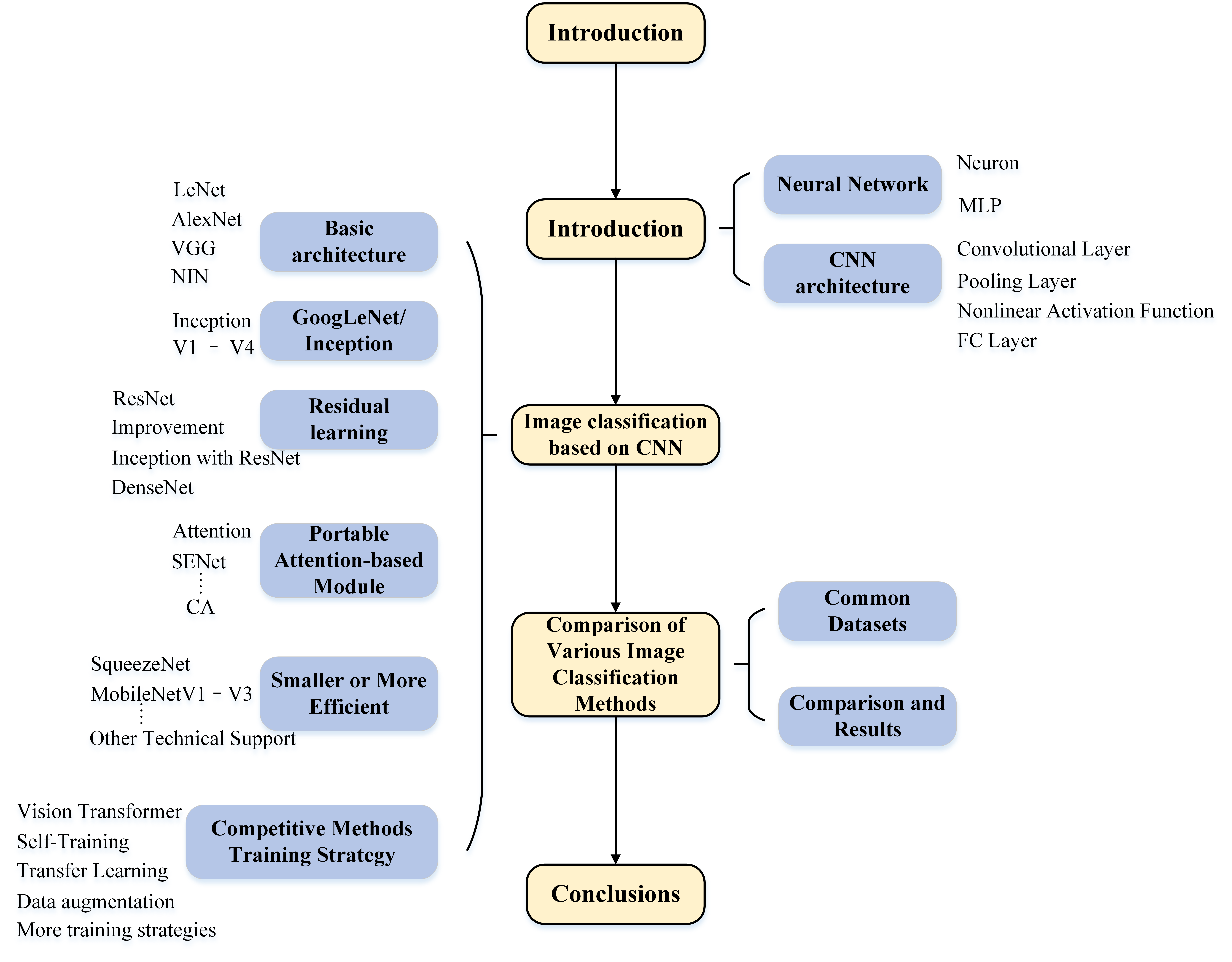
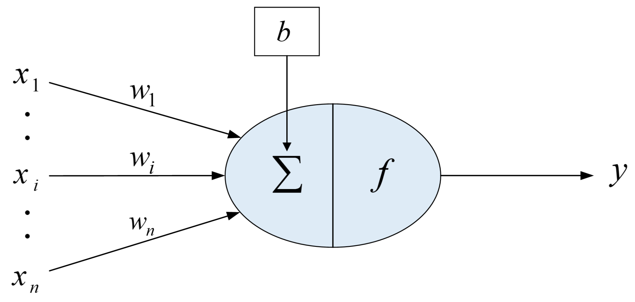
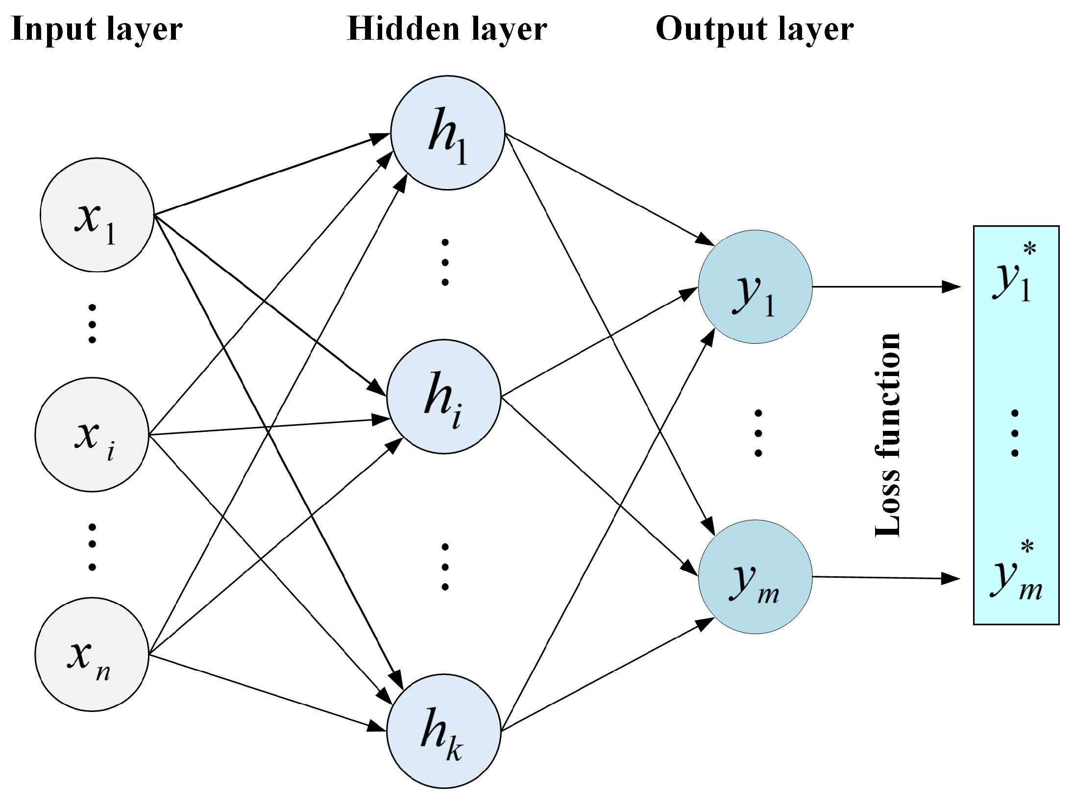
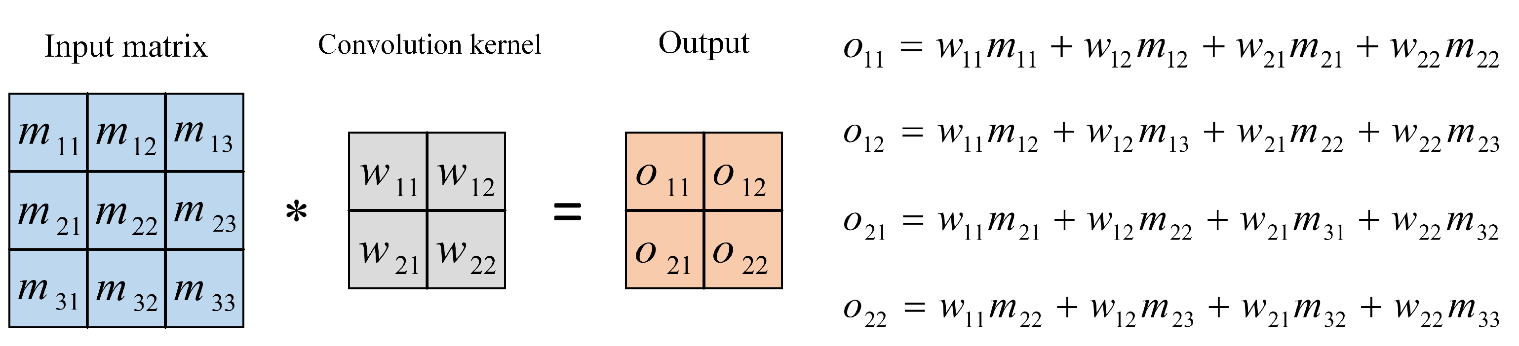
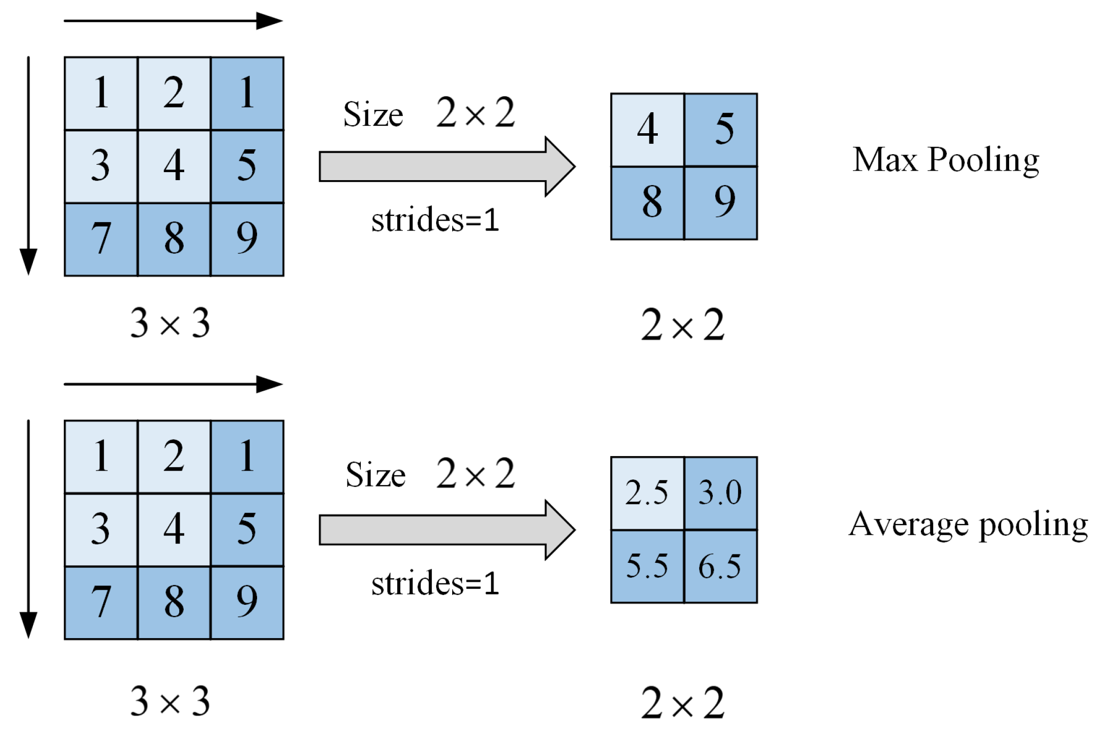
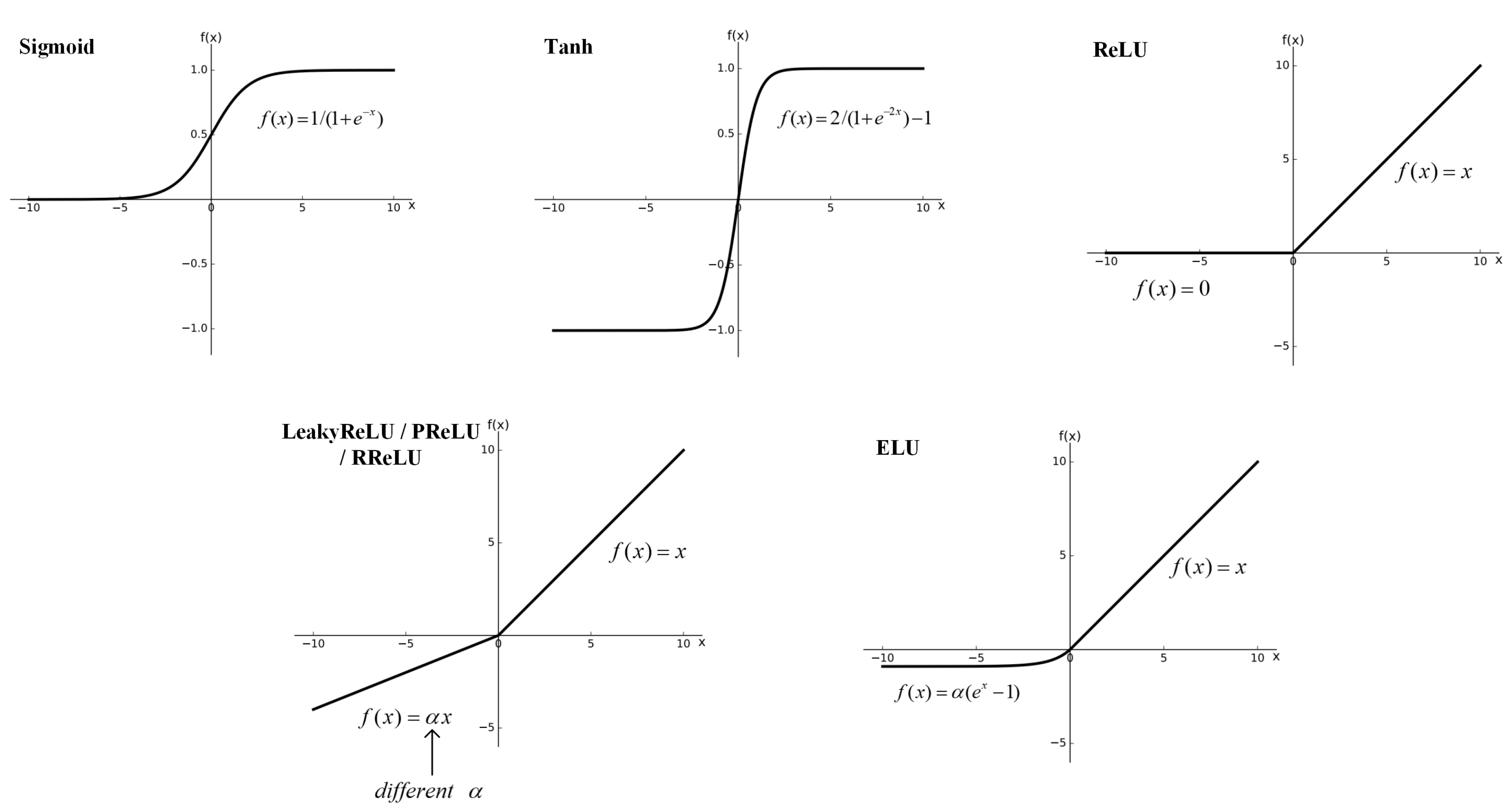
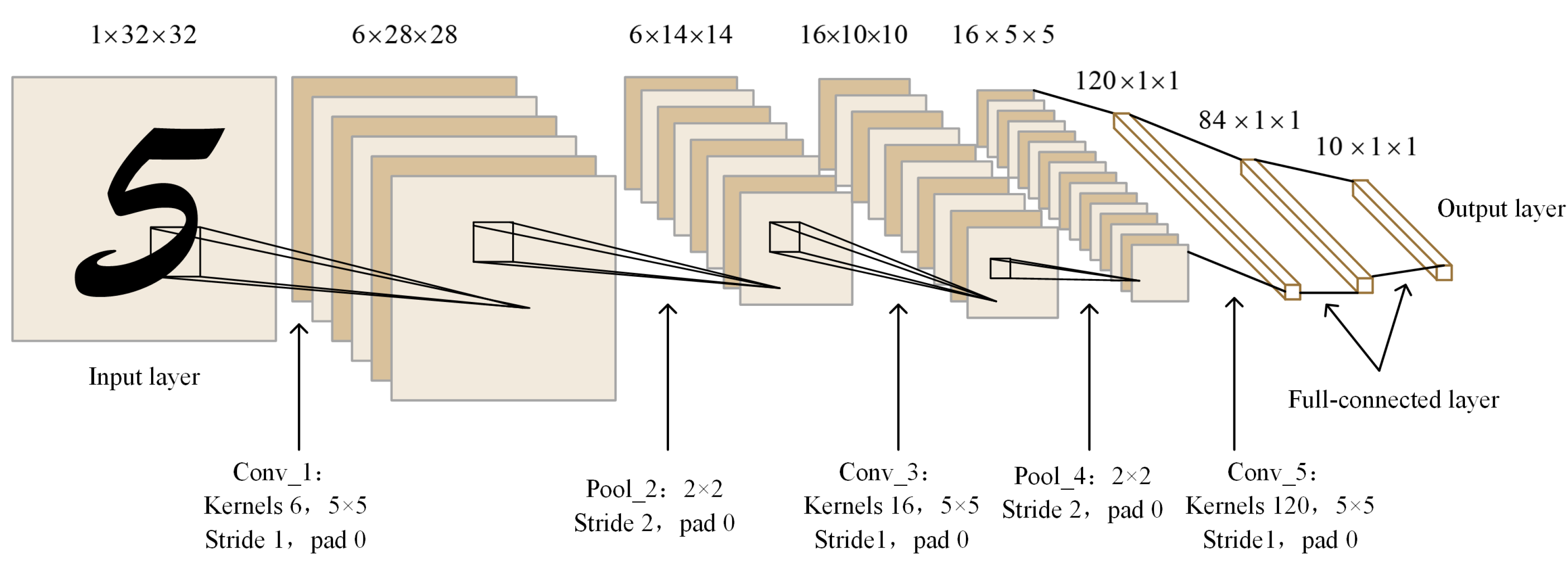
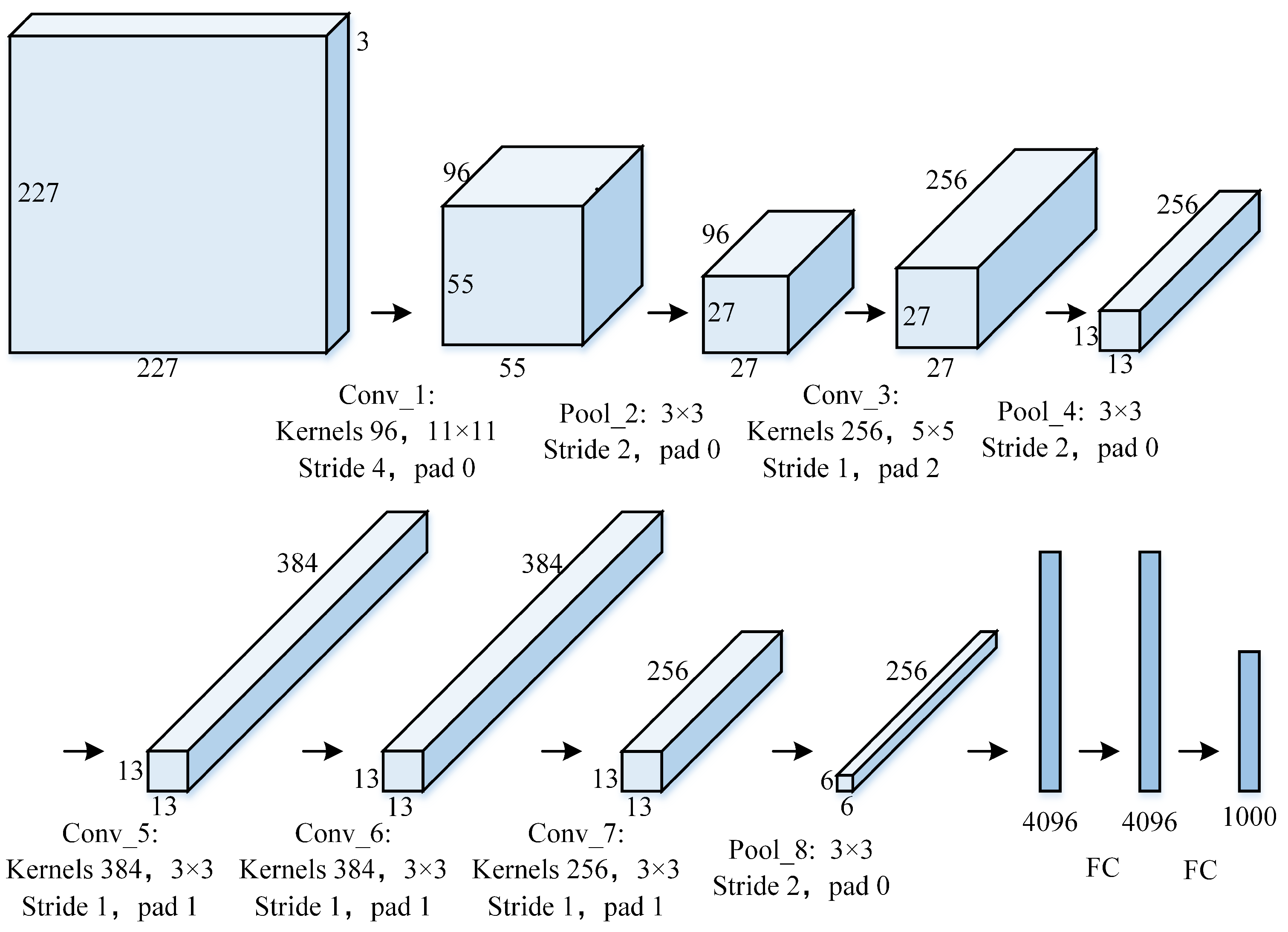
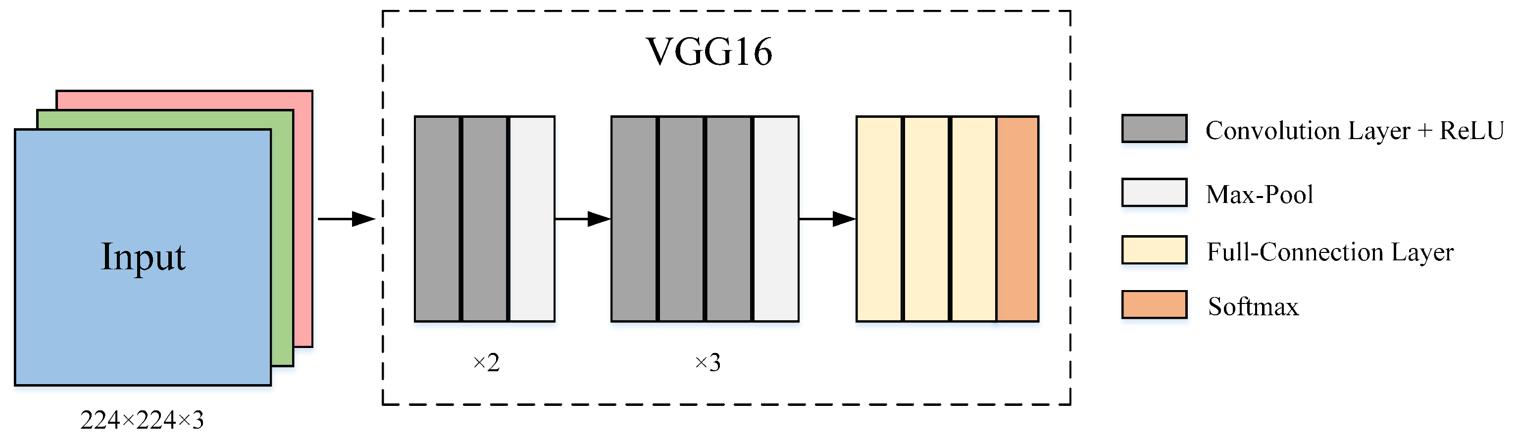
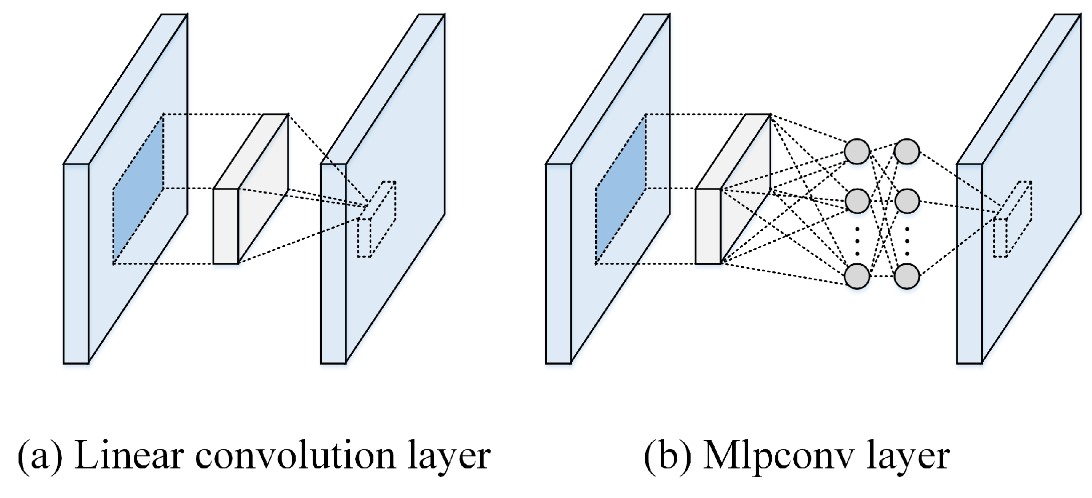
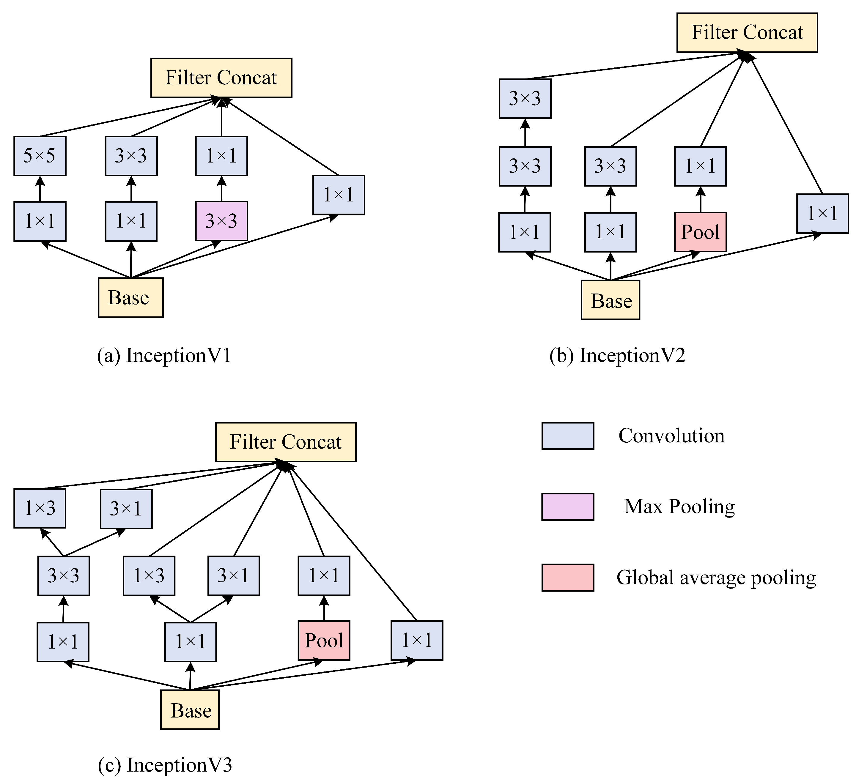
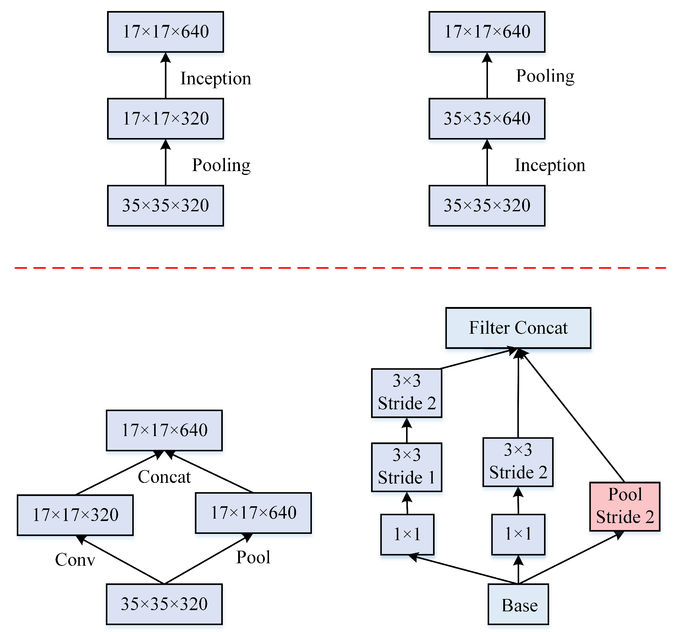
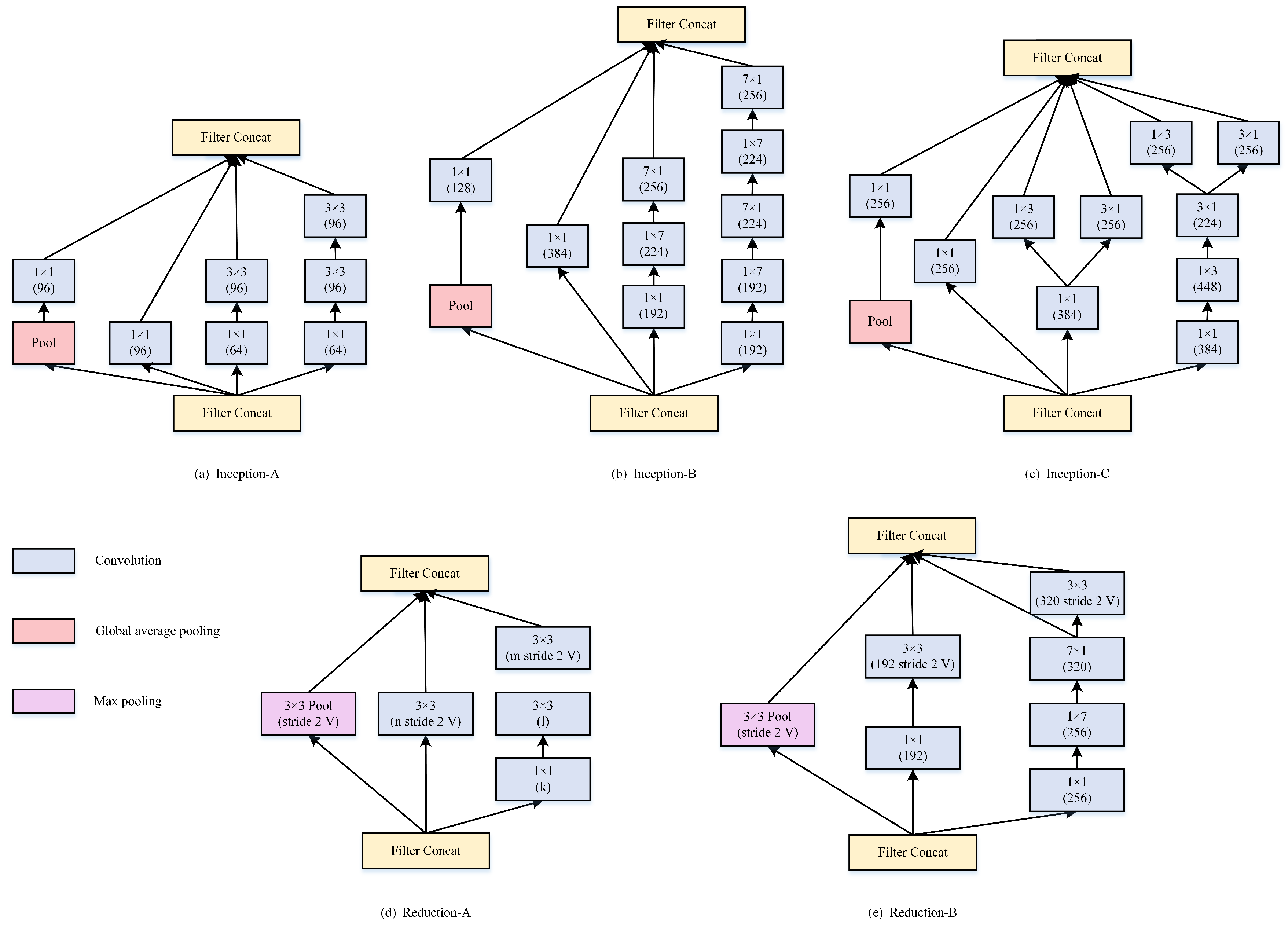
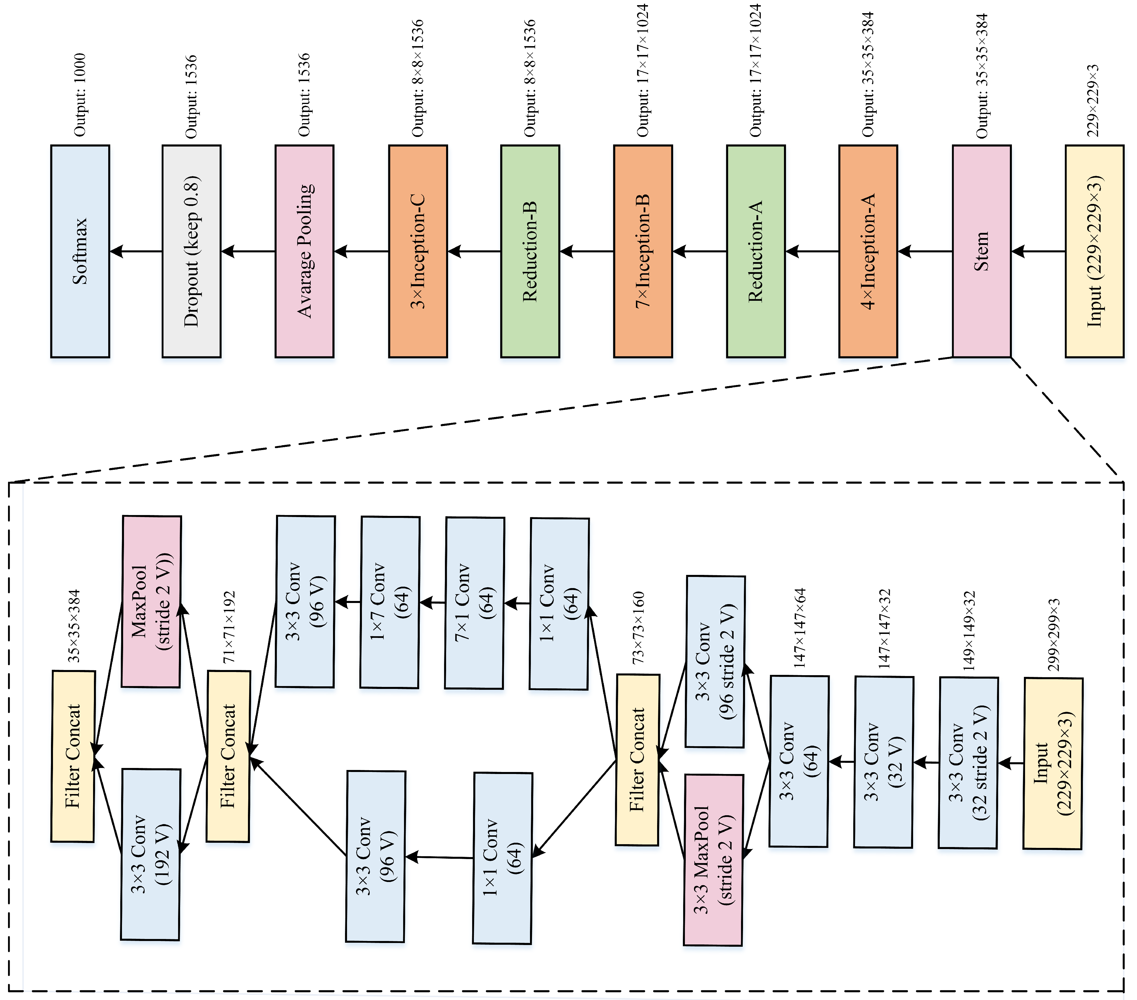
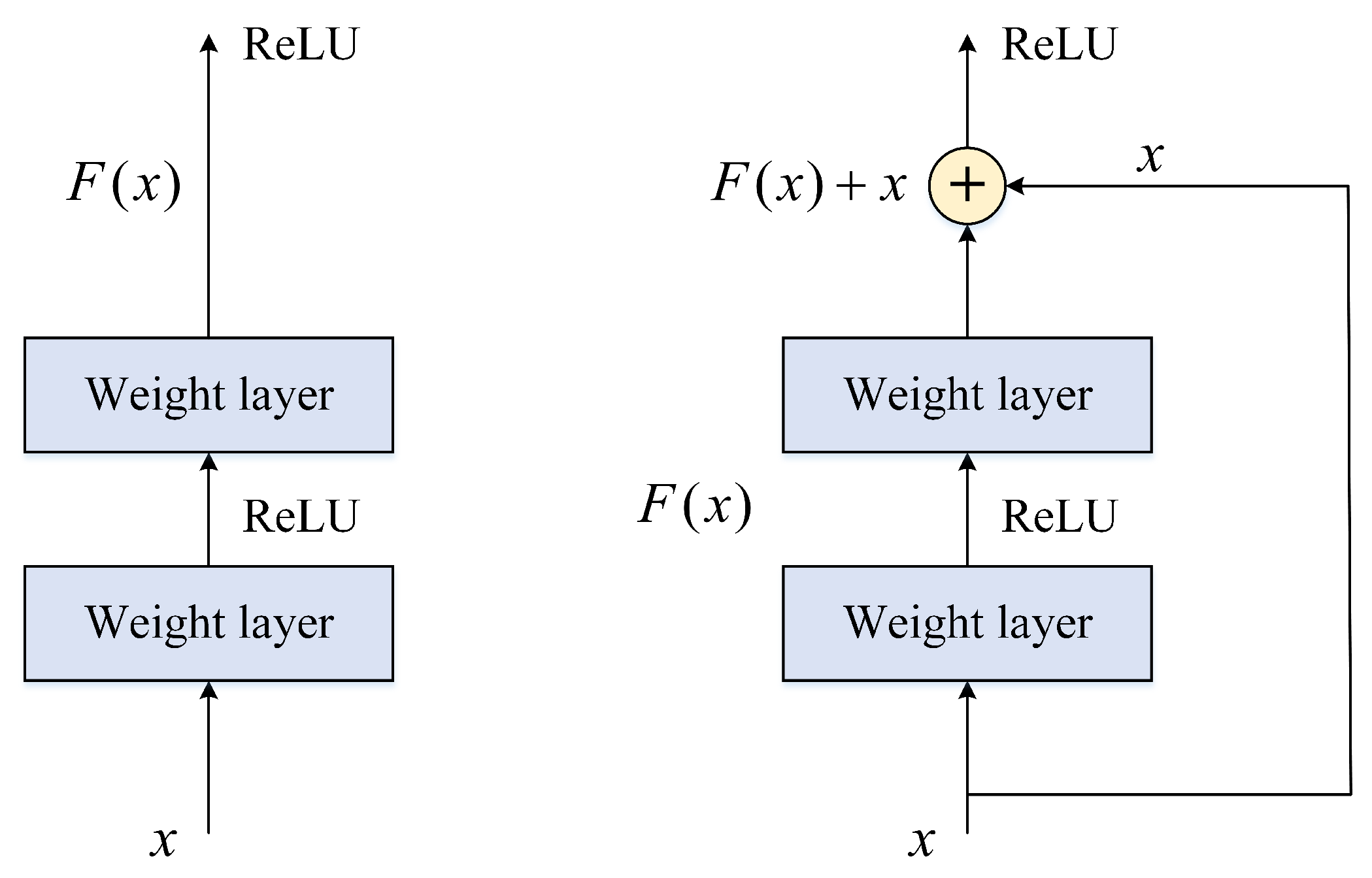
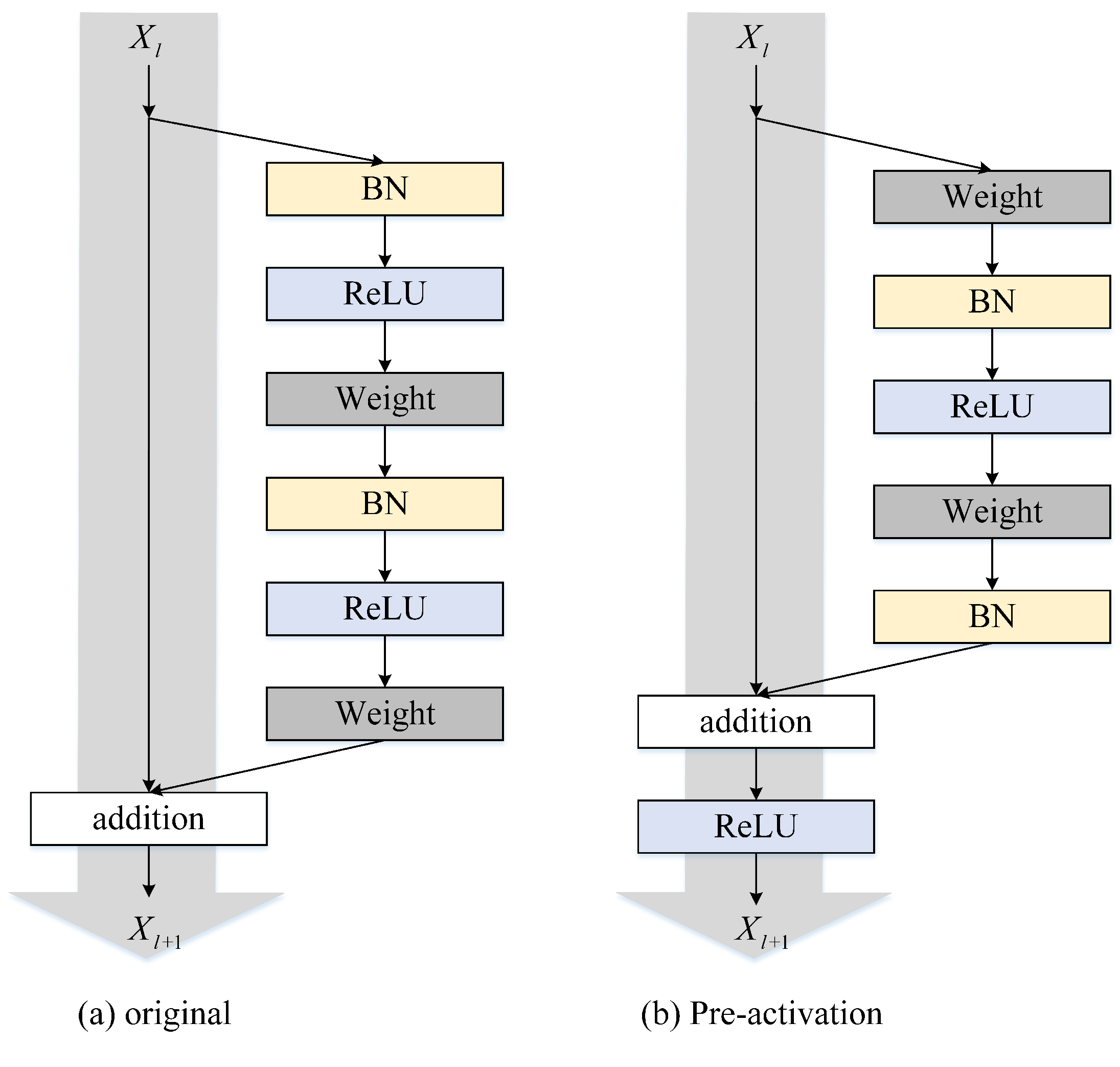
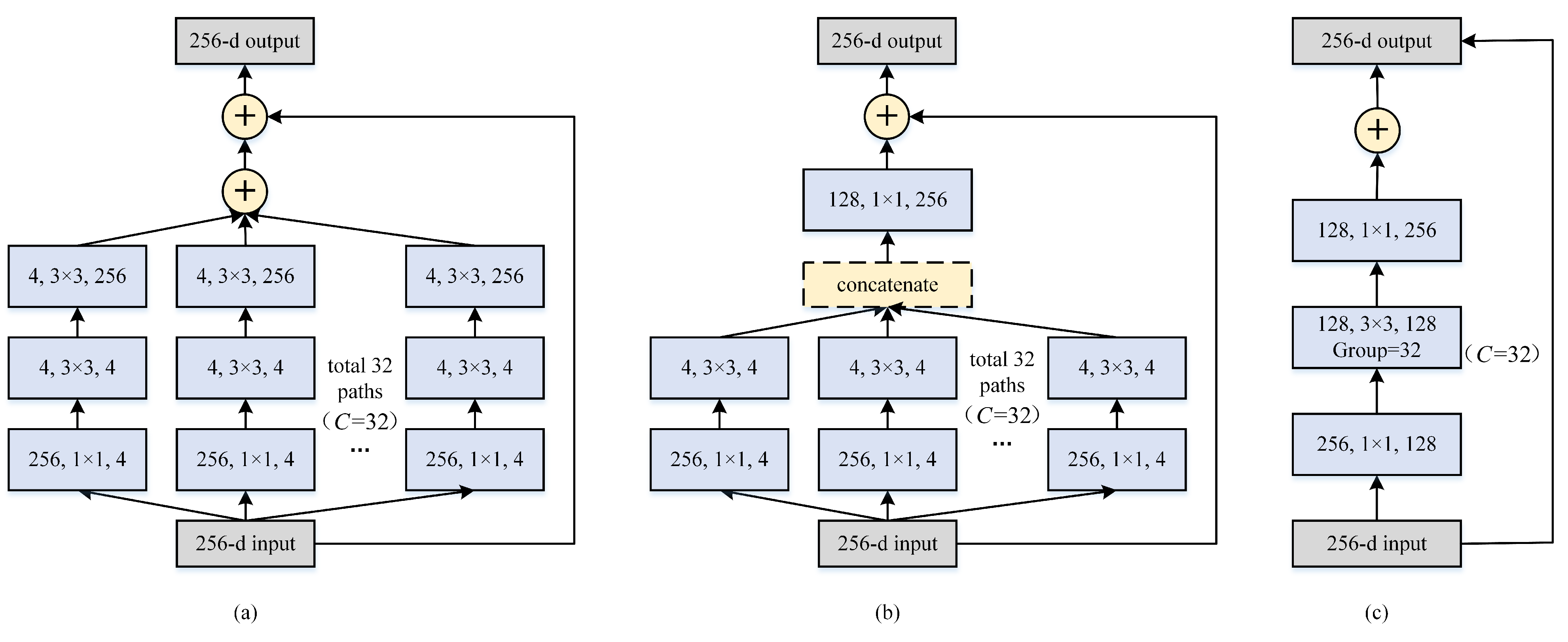
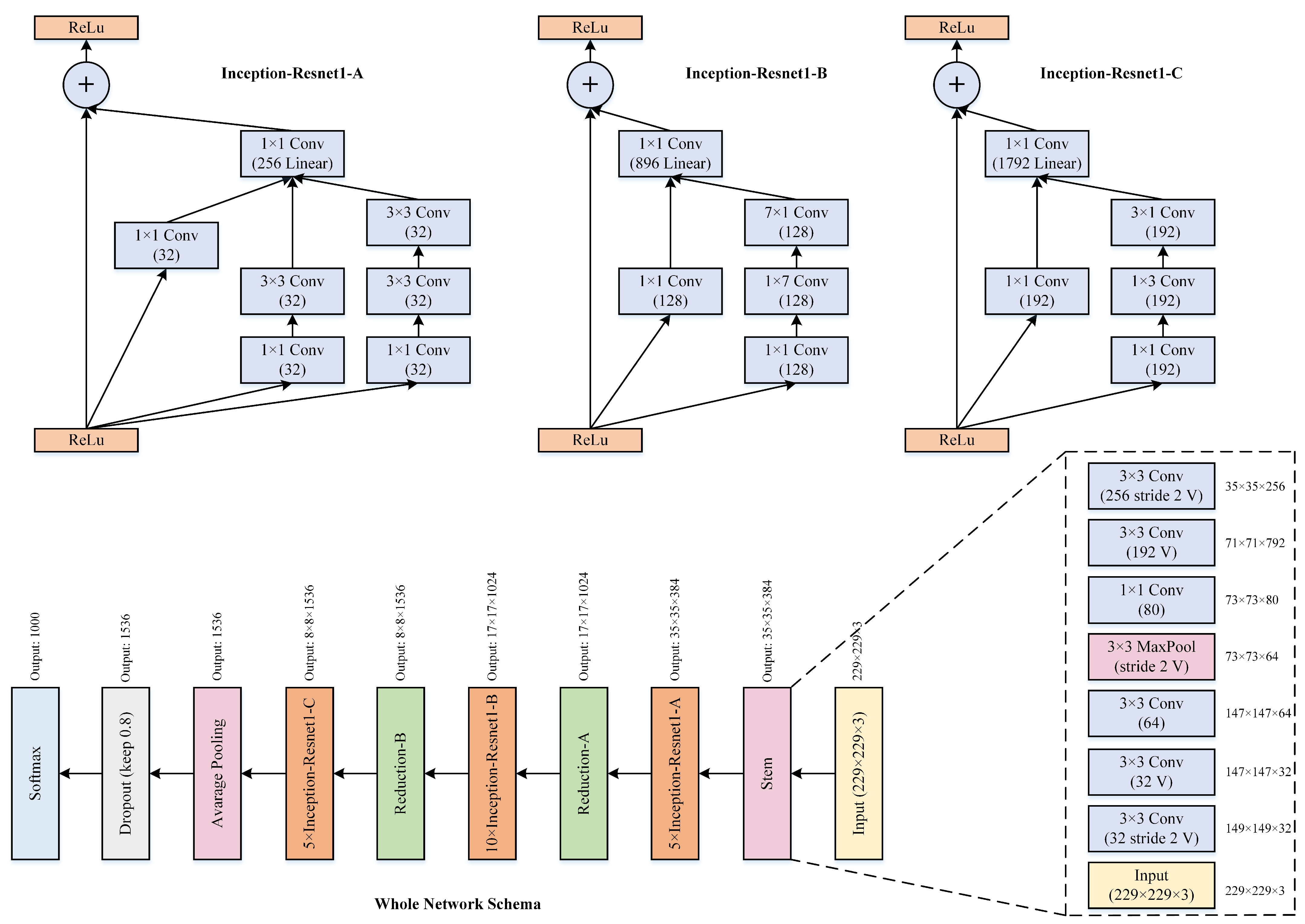
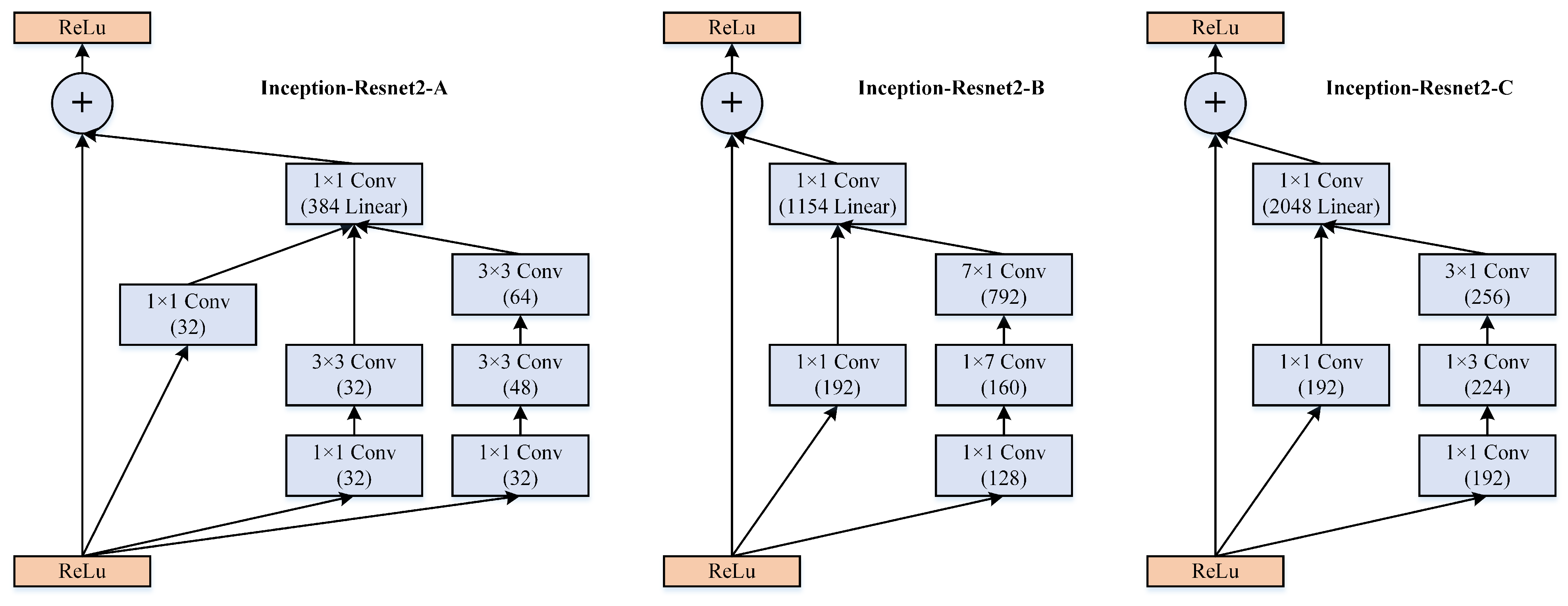
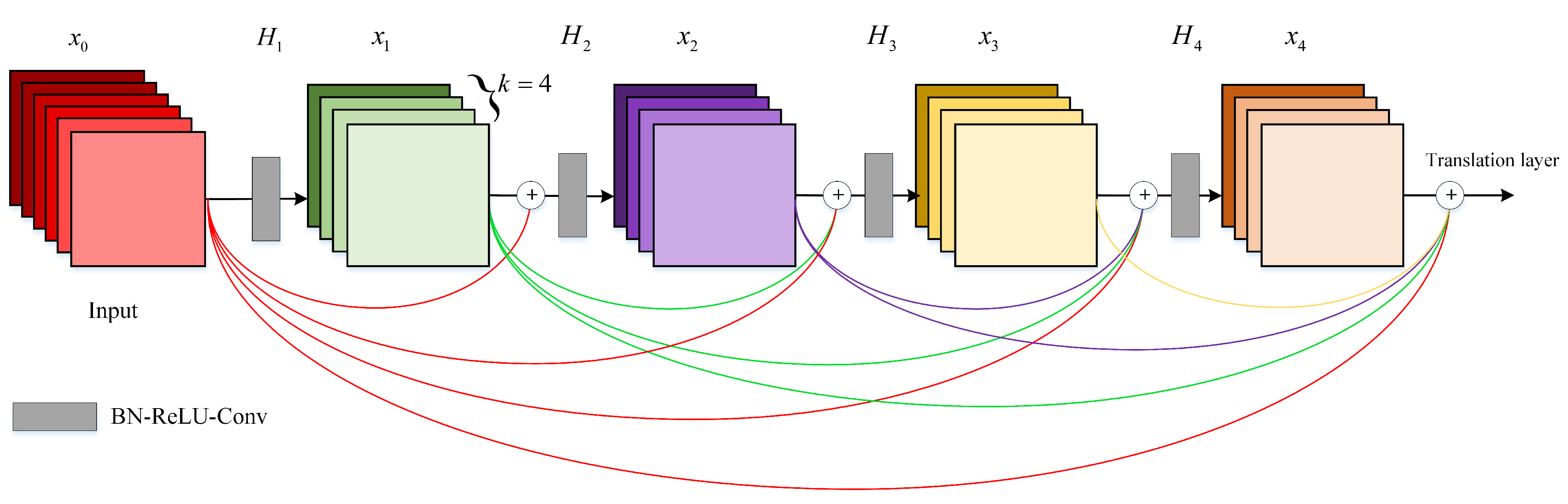
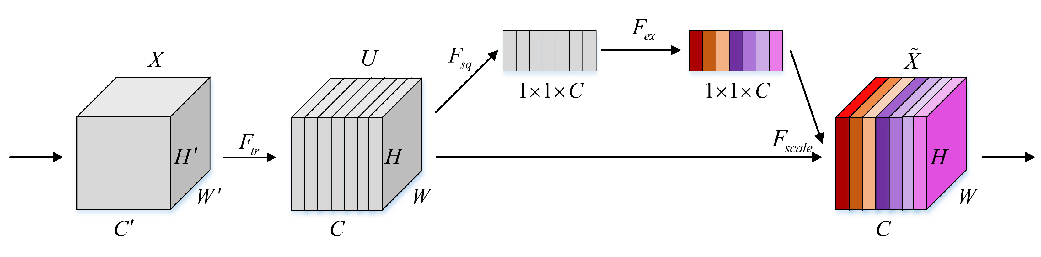
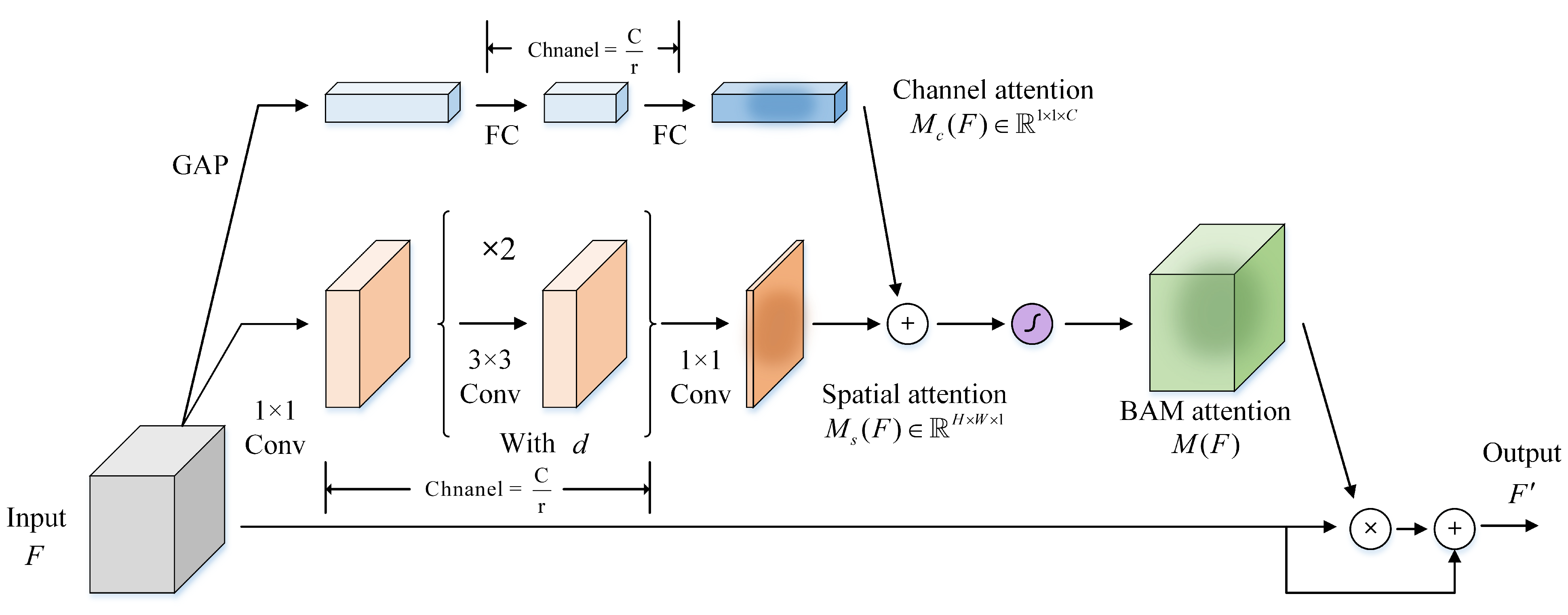
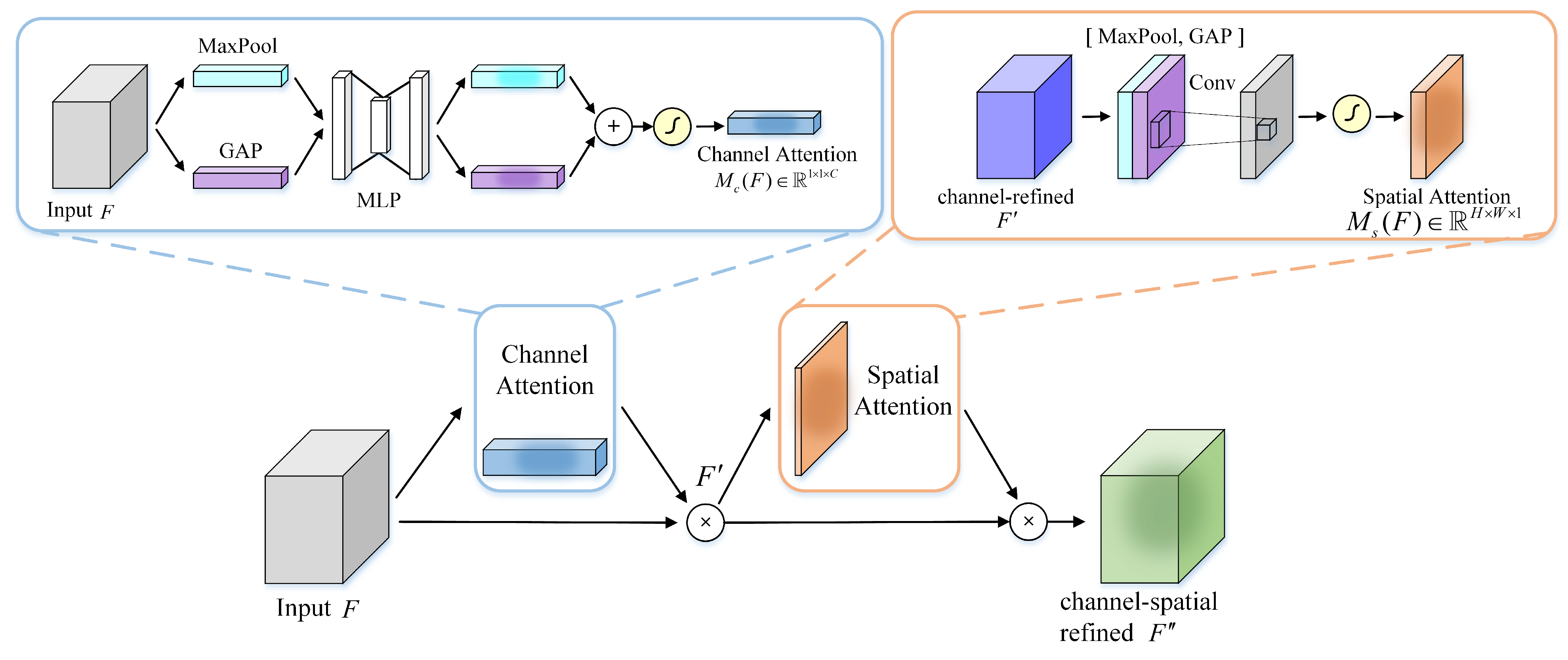
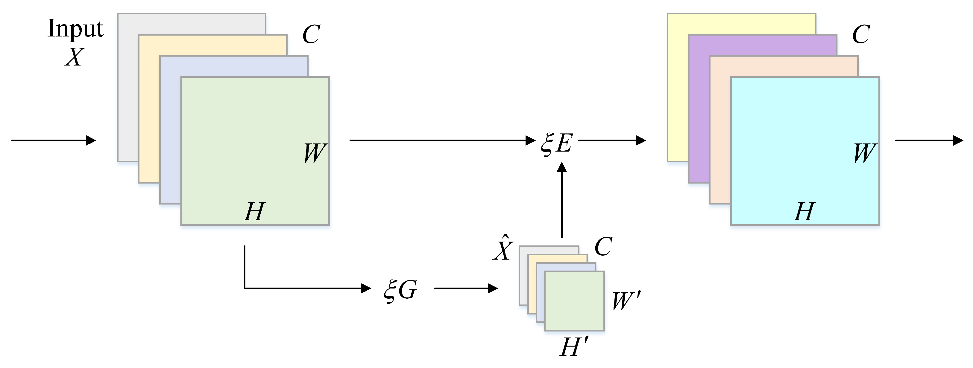
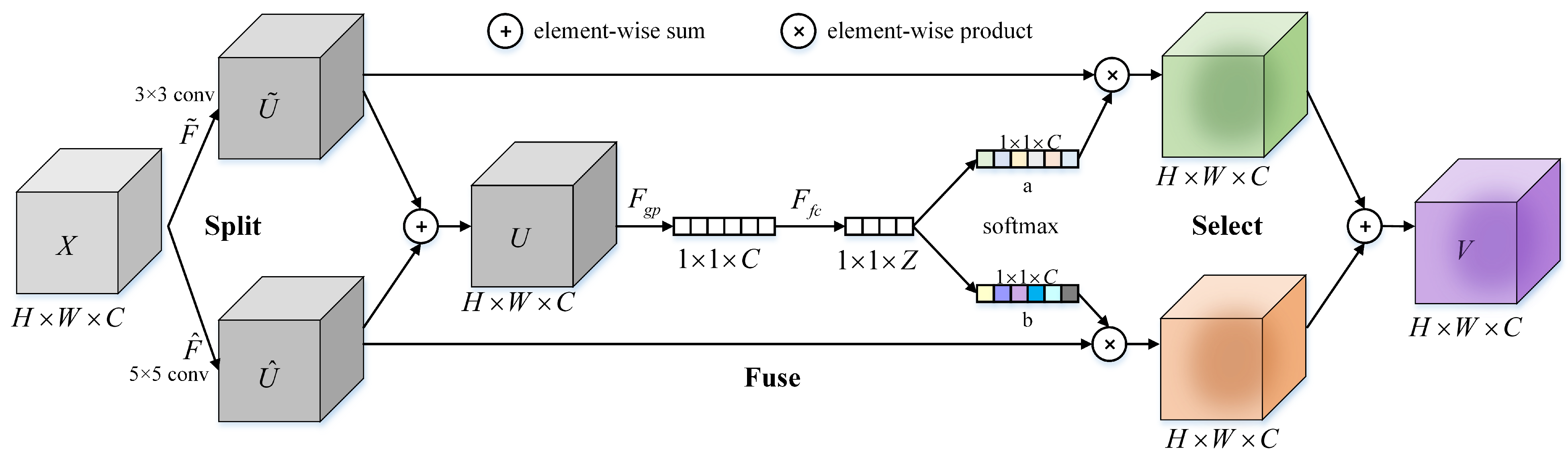
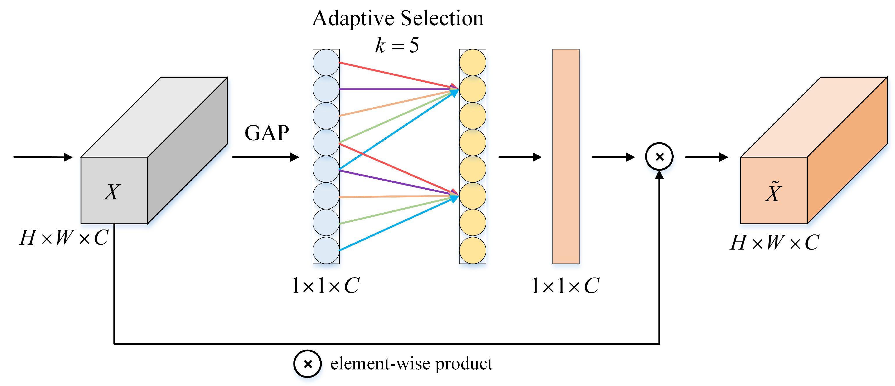
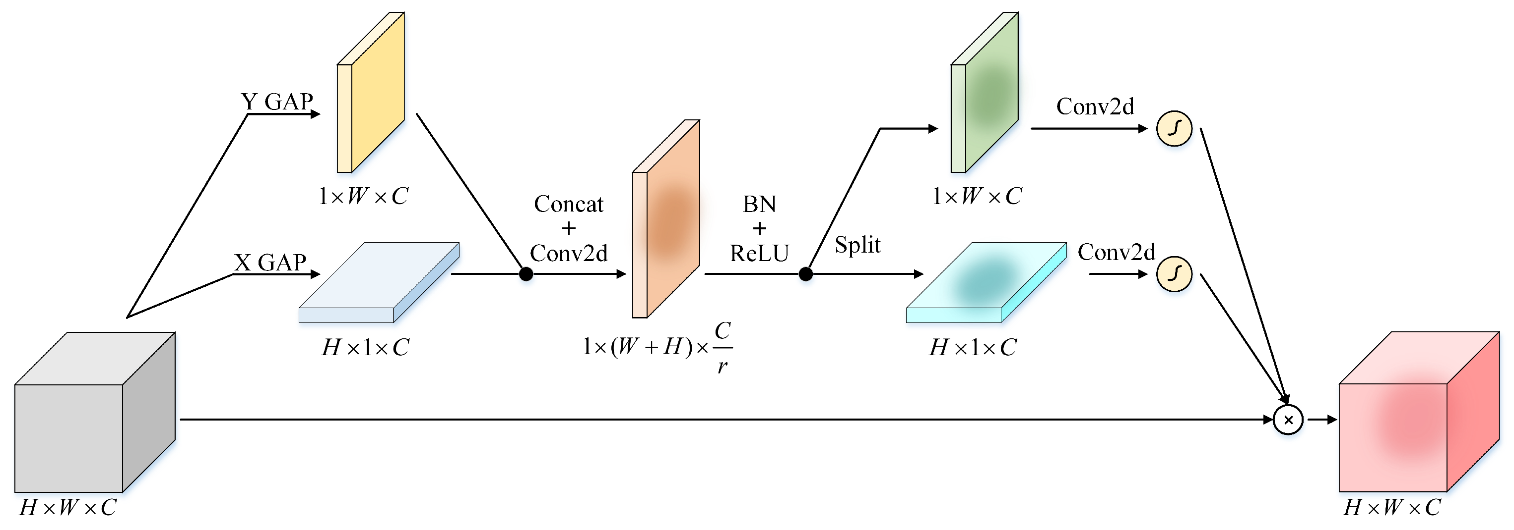
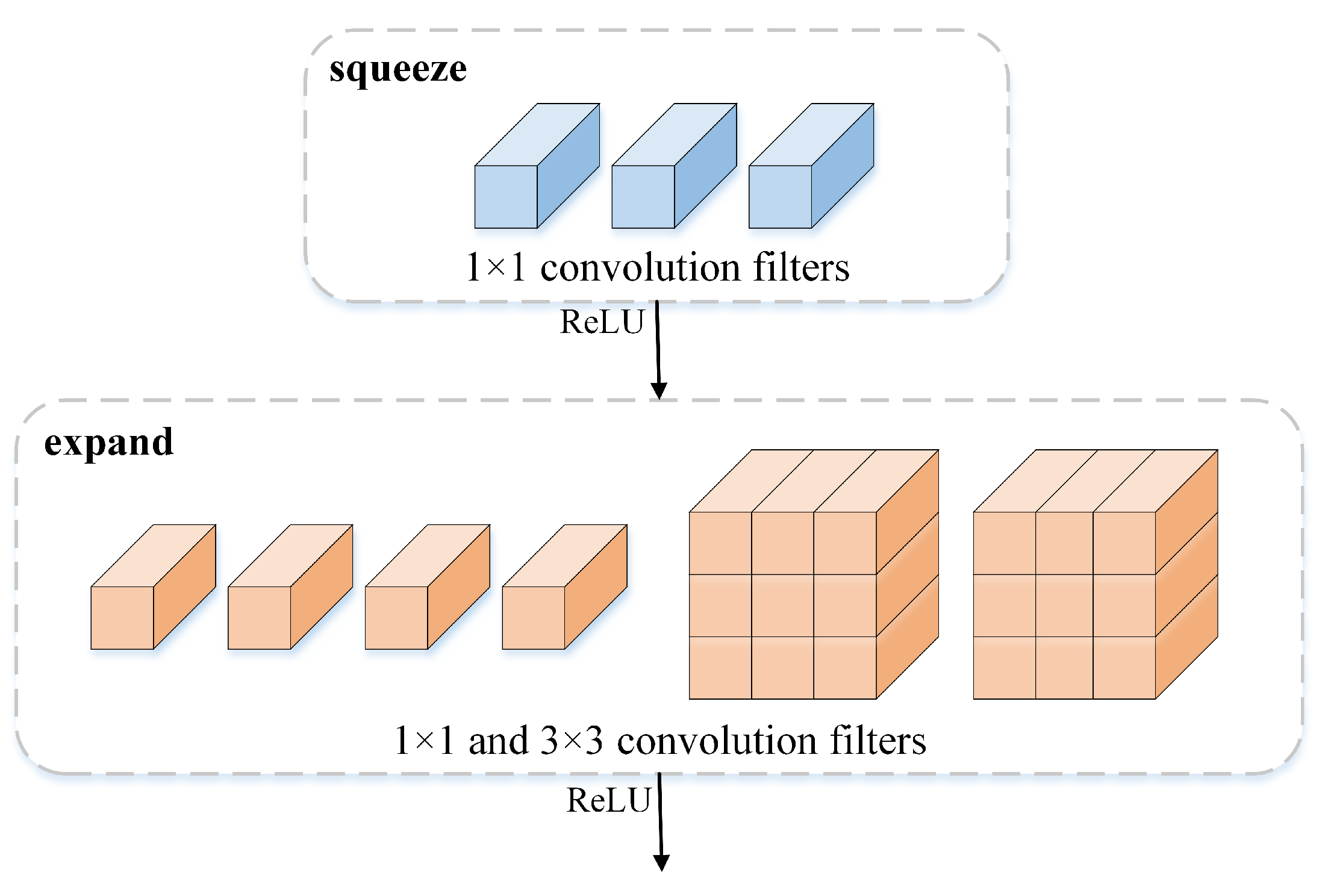
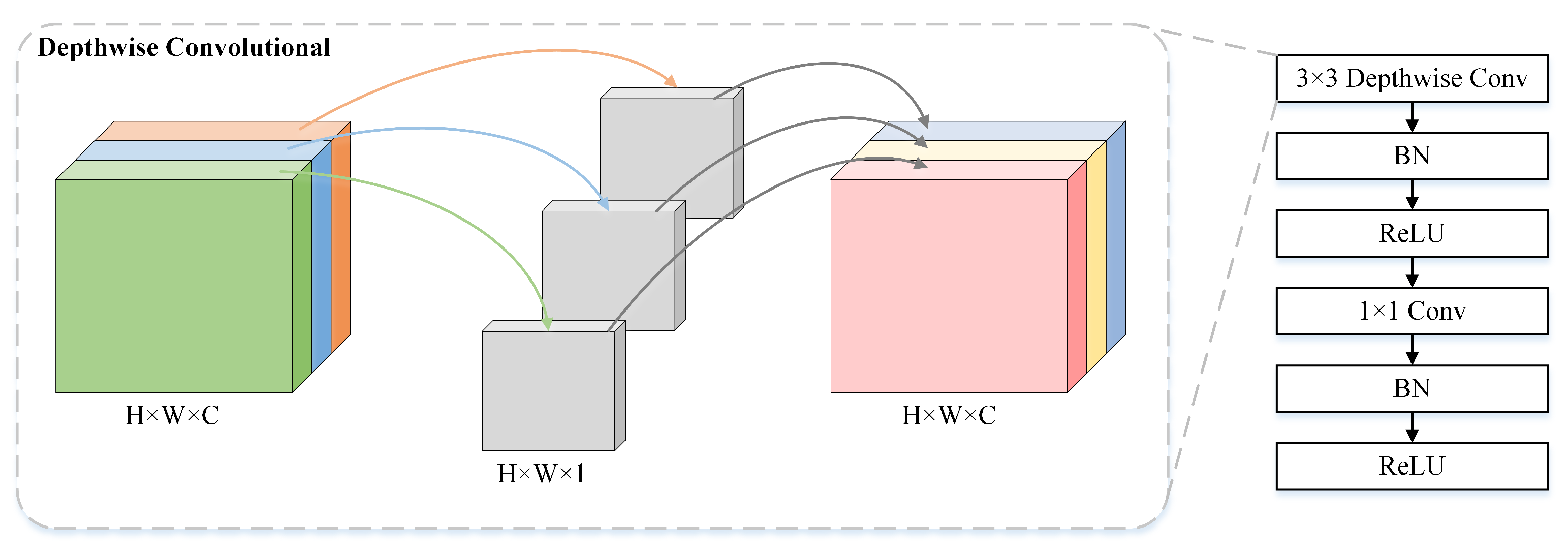
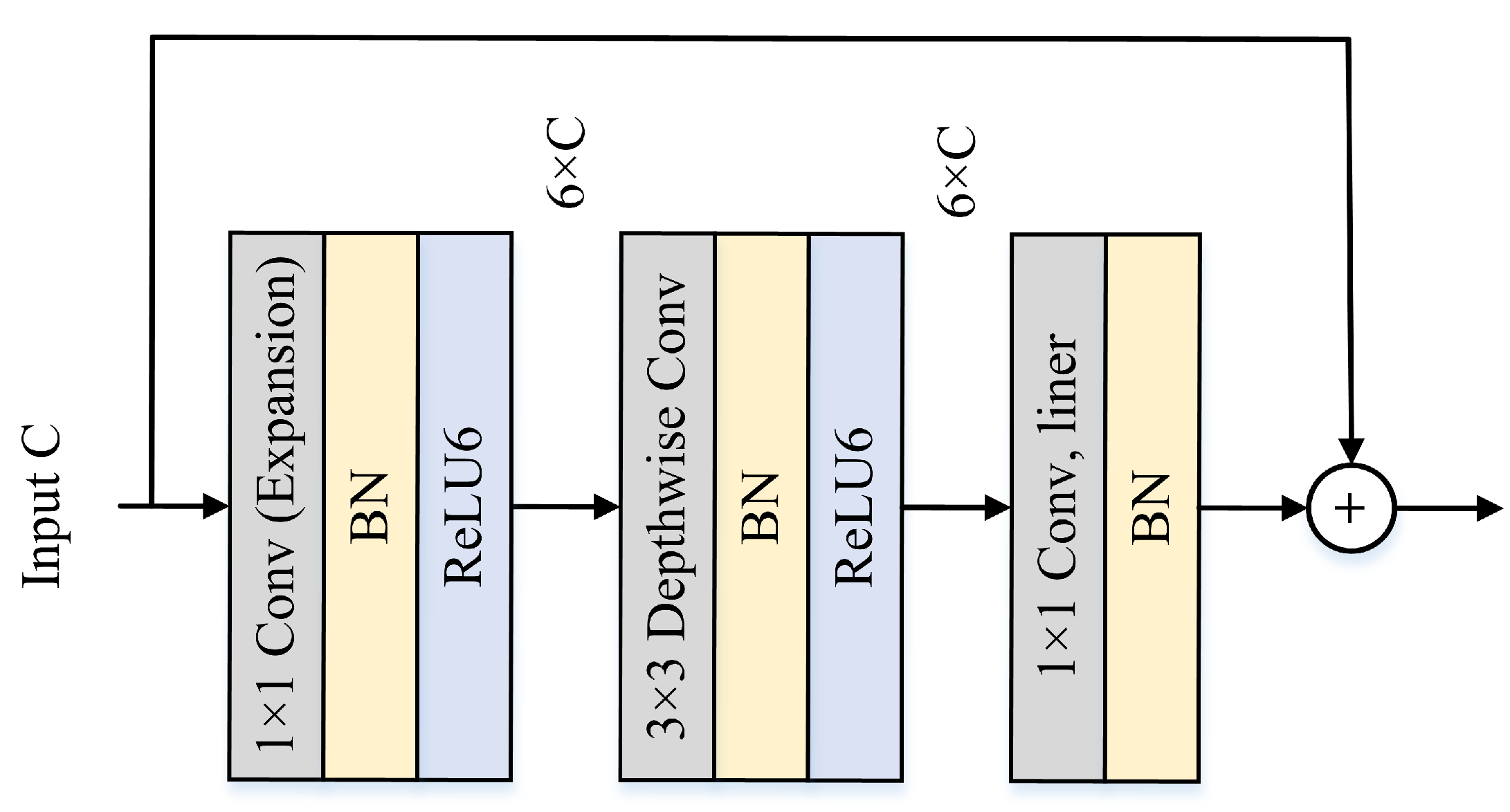
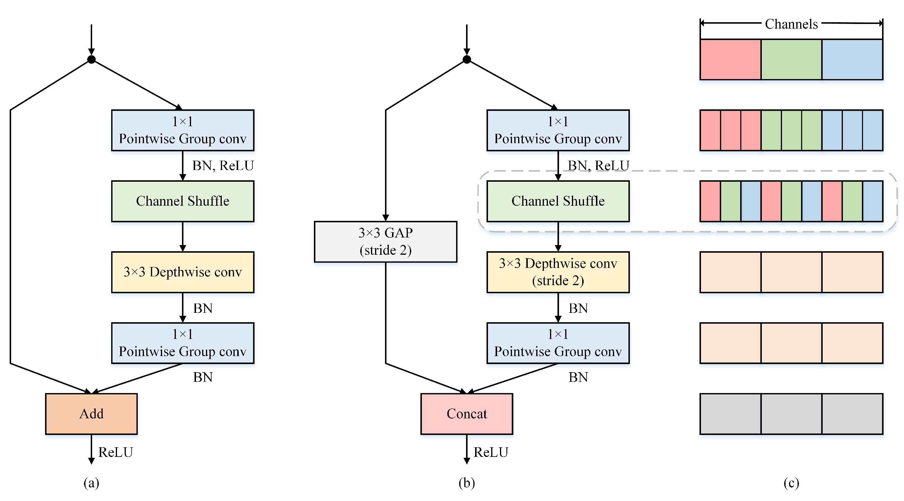
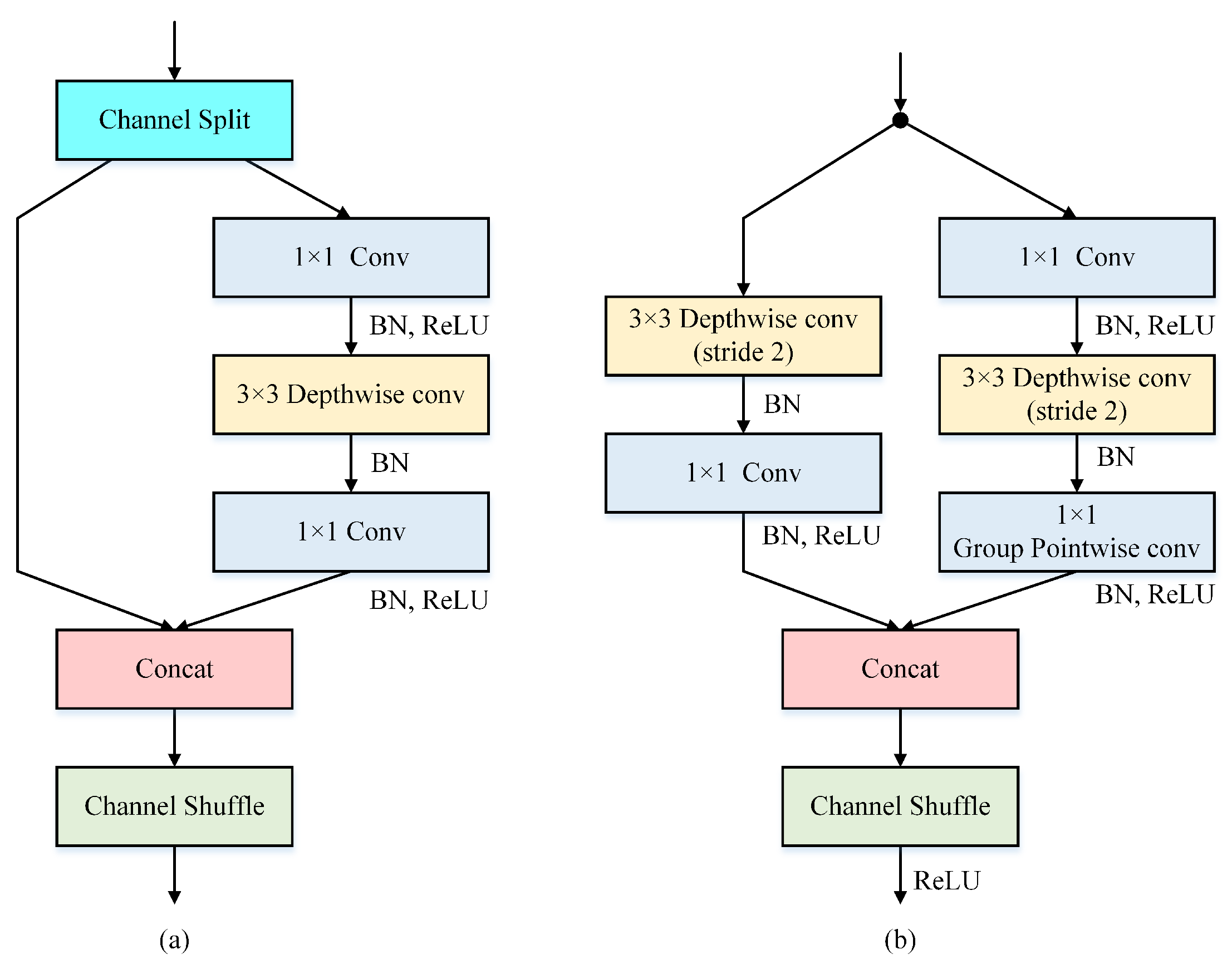
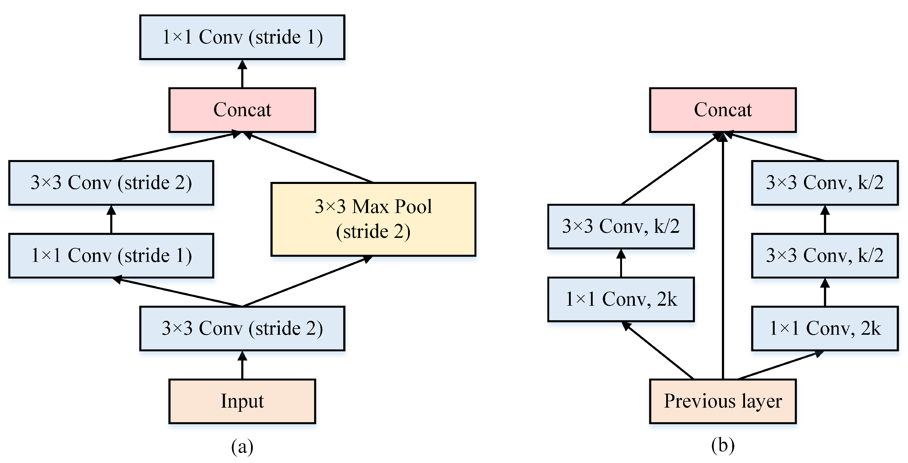
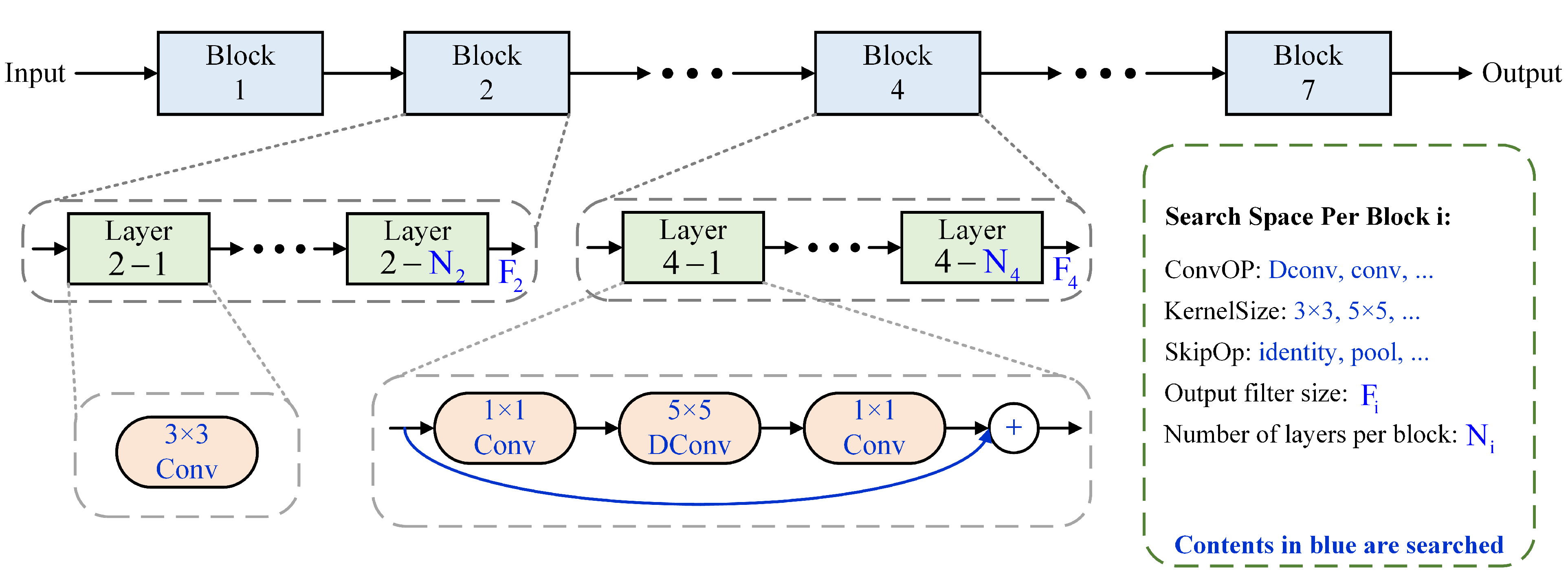
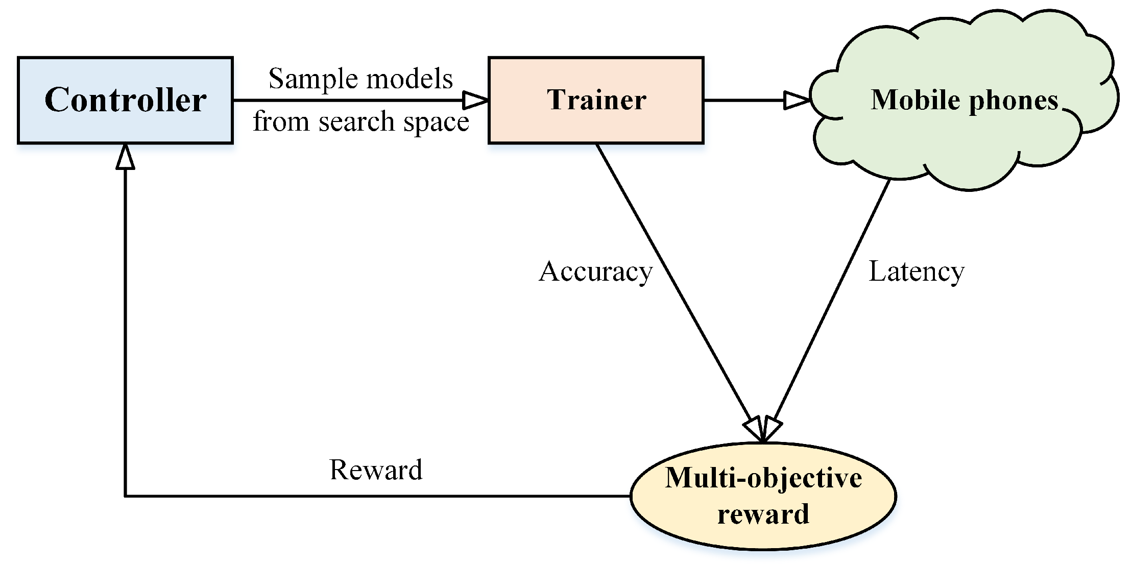
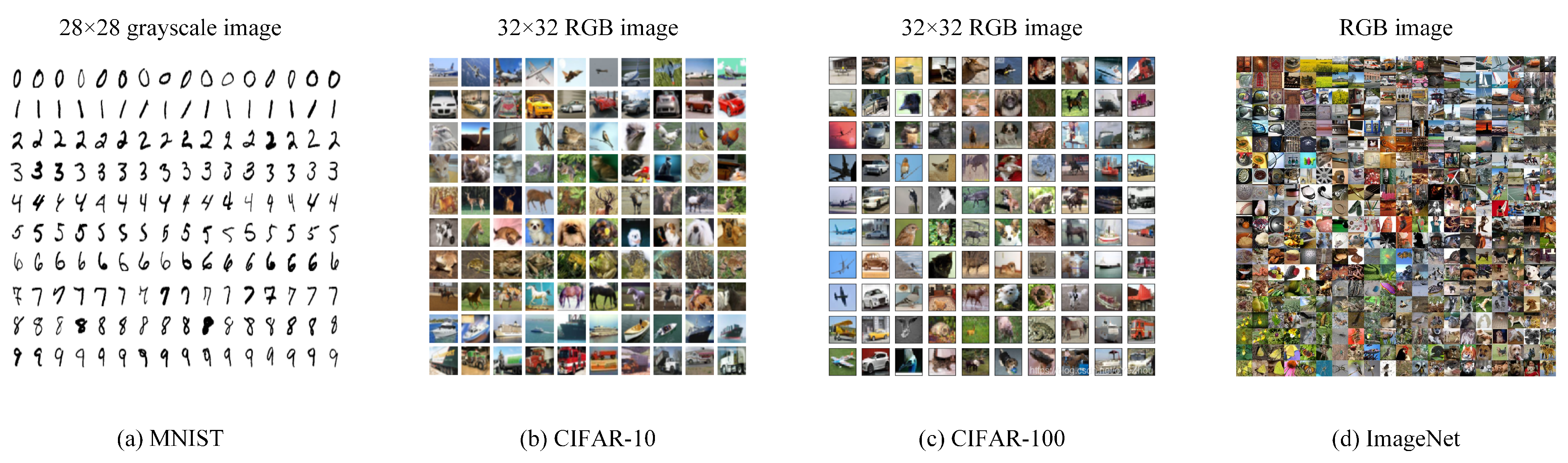
| Loss Function | Equation | Characteristic |
|---|---|---|
| L1 (MAE) | This function is widely used in regression problems. L1 Loss is called mean absolute error (MAE) | |
| L2 (MSE) | This function is widely used in regression problems. L2 Loss is called mean square error (MSE) | |
| Softmax + Cross-Entropy | This function usually employed as a substitution of the MSE in multi-class classification problems. It is also commonly used in CNN models |
| Name | Method | Characteristics |
|---|---|---|
| Batch Gradient Descent (BGD) | It calculates the gradient of the whole training set and subsequently uses this gradient to update the parameters. | 1. For a small-sized dataset, the CNN model converges faster and creates an extra-stable gradient using BGD. 2. Generally not suitable fora large training dataset 3. It requires a substantial amount of resources. |
| Stochastic Gradient Descent (SGD) | It samples by arbitrarily selecting part of the training sample. | 1. For a large-sized training dataset, this technique is both more memory-effective and much faster than BGD. 2. Randomness and noise are introduced due to its frequent updates. Its convergence is not stable, but the expectation is still equal to the correct gradient descent. |
| Mini-batch Gradient Descent | It partitionss the training samples into several mini-batches, and then parameter updating is performed following gradient computation on every mini-batch. | This method combines the technical advantages of SGD and SGD, which has a steady convergence, more computational efficiency and extra memory effectiveness. |
| Momentum | It introduces a momentum parameter into SGD that accumulates historical gradient information. | When training falls into a local minimum, the gradient information with momentum can help the network escape and find the global minimum |
| Adaptive Moment Estimation (Adam) | It calculates an adaptive learning rate for each parameter in the model | The advantages of momentum and RMSprop are combined. It is widely used in deep learning and represents the latest trend of optimization. |
| Model | Year | Depth/Version | Data Set | BFLOPs | Params | Accuracy(%) ImageNet, Top-1 | Accuracy(%) CIFAR 10 | Accuracy(%) CIFAR 100 | Characteristics | Approach |
|---|---|---|---|---|---|---|---|---|---|---|
| AlexNet | 2012 | 8 | ImageNet | - | 60M | 63.3 | - | - | ReLU and Dropout | CNN |
| NIN | 2013 | 3 | CIFAR 10/100 | - | - | 91.19 | 64.33 | “mlpconv” layer and GAP | CNN | |
| VGGNet | 2014 | 16 | ImageNet | - | 138M | 74.4 | - | - | Small filter size, Blocks of layers | CNN |
| InceptionV1 (GoogLeNet) | 2014 | 22 | ImageNet | 1.45 | 6.8M | - | - | - | Inception block with different filter size | CNN |
| InceptionV2 | 2015 | - | ImageNet | 1.94 | 11.2M | 74.8 | - | - | BN, Small filter size | CNN |
| InceptionV3 | 2015 | 48 | ImageNet | 5.73 | 24M | 78.8 | - | - | Using small filter size to burn less computational power | CNN |
| ResNet | 2015 | 50, 101 110, 1202 | ImageNet CIFAR 10/100 | 3.86, 7.57 | 25.6M, 44.5M 1.7M, 10.2M | 77.15, 78.25 | 93.57, 92.07 | 74.84, 72.18 | Residual learning | CNN |
| ResNet (pre-activation) | 2016 | 200 164, 1001 | ImageNet CIFAR 10/100 | - | 64.7M 1.7M, 10.2M | 79.9 | 93.63, 95.38 | -, 77.29 | pre-activation structure | CNN |
| Stochastic Depth | 2016 | 110, 1202 | CIFAR 10/100 | - | 1.7M, 10.2M | - | 94.77, 95.09 | 75.09, - | Stochastic delete some layers | CNN |
| WRN | 2016 | 50 16, 28 | ImageNet CIFAR 10/100 | - | 68.9M 11.0M, 36.5M | 78.1 | 95.74, 96.00 | 79.57, 80.75 | Wider and shallower | CNN |
| DRN-A | 2016 | 50 | ImageNet | - | 25.6M | 78.7 | - | - | Using Dilated convolutions to increase the receptive field | CNN |
| DenseNet | 2016 | 264 190 | ImageNet CIFAR 10/100 | 6 | - 25.6M | 77.85 | 96.54 | 82.82 | Each layer connects to every other layer | CNN |
| Inception-ResNet-v2 | 2016 | 164 | ImageNet | 11.75 | 55.8M | 80.1 | - | - | Combined residual connection and Inception | CNN |
| Xception | 2016 | 71 | ImageNet | 8.4 | 22.8M | 79 | - | - | Combined residual connection and Inception Depthwise separable convolutions | CNN |
| InceptionV4 | 2016 | 70 | ImageNet | 13 | 48M | 80 | - | - | Divided transform and integration concepts | CNN |
| ResNeXt | 2016 | 101(32×4d) 101(64×4d) | ImageNet | 7.508 32 | 44.18M 83.6M | 78.80 80.90 | - | - | Combined residual connection and Inception Grouped convolution | CNN |
| DropBlock | 2018 | 50 | ImageNet | 3.86 | 25.6M | 78.35 | - | - | Dropout the units with a contiguous region | CNN |
| Attention | 2017 | 92 92, 452 | ImageNet CIFAR 10/100 | 10.4 | 51.3M 1.9M, 8.6M | 80.50 - | - 95.01, 96.10 | - 78.29, 79.55 | Stacked attention modules based on residual connections | CNN +Attention’ |
| PolyNet | 2017 | - | ImageNet | 34.7 | 92M | 81.3 | - | - | Combined residual connection and Inception | CNN |
| SENet | 2017 | 101 152 | ImageNet | 8.00 42 | 49.2M 146M | 81.36 82.72 | - | - | Channel attention Implantable lightweight module | CNN +Attention’ |
| DPN | 2017 | 131 | ImageNet | 16 | - | 81.38 | - | - | Combination of residual learning and dense connection | CNN |
| NASNet-A | 2017 | - | ImageNet | 23.8 | 88.9M | 82.7 | - | - | NASNet search space | CNN +NAS |
| PNASNet | 2017 | - | ImageNet | 25 | 86.1M | 82.9 | - | - | Smaller NASNet search space Sequential Model-based Optimization | CNN +NAS |
| ResNeXt (32×4d) + BAM | 2018 | 101 | ImageNet | 8.05 | 44.6M | 80.85 | - | - | Channel attention and spatial attention Implantable lightweight module | CNN +Attention’ |
| ResNeXt (32×4d) + CBAM | 2018 | 101 | ImageNet | 7.519 | 49.2M | 80.58 | - | - | Channel attention and spatial attention Implantable lightweight module | CNN +Attention’ |
| AmoebaNet-A | 2018 | - | ImageNet | 23.1 104 | 86.7M 469M | 82.8 83.9 | - | - | NASNet search space and genetic algorithm | CNN +NAS |
| GPipe | 2018 | - | ImageNet CIFAR 10/100 | - | 557M | 84.3 | 99 | 91.3 | Using Pipeline Parallelism to train effectively | CNN |
| ResNet + GE | 2019 | 101 | ImageNet CIFAR 10/100 | 7.59 | 58.4M - | 79.26 - | - 95.07 | - 79.15 | Feature context exploitation Implantable lightweight module | CNN +Attention’ |
| ECA-Net | 2019 | 101 | ImageNet | 7.35 | 42.45M | 78.65 | - | - | No channel dimensionality reduction Portable lightweight modul | CNN +Attention’ |
| SKNet | 2019 | 101 29 | ImageNet CIFAR 10/100 | 8.46 | 48.9M 27.7M | 79.81 - | - 96.53 | - 82.67 | Adaptively adjust receptive field Implantable lightweight module | CNN +Attention’ |
| GSoP-Net | 2019 | 50 | ImageNet | 6.56 | 58.65M | 78.81 | - | - | Global Second-order Pooling Implantable lightweight module | CNN +Attention’ |
| EfficientNetV1 | 2019 | B0 - B7, L2 | ImageNet | 0.39, 0.70, 1.0, 1.8, 4.2, 9.9, 19, 37, - | 5.3M, 7.8M, 9.2M 12M, 19M, 30M 43M, 66M, 480M | 77.1, 79.1, 80.1, 81.6, 82.9, 83.6, 84.0, 84.3, 85.5 | 98.9 (B7) | 91.7 (B7) | Utilizes effective compound coefficient to scale up CNNs | CNN +NAS |
| BiT | 2019 | -L | ImageNet CIFAR 10/100 | - | - | 87.54* | 99.37 | 93.51 | Transfer learning Better training and fine-tuning strategies | CNN Transfer-learning |
| NoisyStudent | 2019 | -L2 | ImageNet | - | 480M | 88.4* | - | - | Self traning / Semi-Supervised add noise to the student | CNN Semi-Supervised |
| FixEfficientNet | 2020 | -B7 -L2 | ImageNet | - | 66.4M 480M | 85.3, 87.1* 85.7, 88.5* | - | - | A training strategy that employs different train and test resolutions | CNN |
| ViT-H/14 | 2020 | -L, -H | ImageNet CIFAR 10/100 | - | 307M, 632M | 87.76*, 88.55* | 99.42, 99.50 | 90.54, 90.72 | Pure transformer model for Computer vision | Vision Transformer |
| Meta Pseudo Labels | 2020 | -L2 | ImageNet | - | 480M | 90.2* | - | - | Self traning / Semi-Supervised Update teacher based on student performance | CNN Semi-Supervised |
| EfficientNetV2 | 2021 | -S, -M, -L | ImageNet CIFAR 10/100 | 8.8, 24, 53 | 22M, 54M, 120M 24M, 55M, 121M | 83.9, 85.1, 85.7 | 98.7, 99.0, 99.1 | 91.5, 92.2, 92.3 | FixRes, Fused-MBConv, NAS | CNN +NAS |
| NFNet | 2021 | F6+SAM, F4+ | ImageNet | 337.28, - | 438.4M, 527M | 86.5, 89.2* | - | - | Adaptive gradient clipping technique, Without Normalization | CNN |
| ViT-G/14 | 2021 | -G/14 | ImageNet | - | 1843M | 90.45* | - | - | Pure transformer model for Computer vision | Vision Transformer |
| CoAtNet | 2021 | -7 | ImageNet | 2586 | 2440M | 90.88* | - | - | Mixed methods, Convolutional + Transformer | CNN + Transformer |
| Model | Year | Version/Baseline | Data Set | MFLOPs | Params | Accuracy(%) Top-1 | CPU Latency | Characteristics | Approach |
|---|---|---|---|---|---|---|---|---|---|
| SqueezeNet | 2016 | - | ImageNet | 1700 | 1.25M | 57.5 | - | Decreased 3×3 conv, deep compression | CNN |
| MobileNetV1 | 2017 | 1.0 | ImageNet | 569 | 4.2M | 70.6 | 113ms | Depthwise separable convolution | CNN |
| ShuffleNetV1 | 2017 | 2×(g=3), +SE | ImageNet | 527 | - | 75.3 | - | Group pointwise convolution, channel shuffle | CNN |
| PeleeNet | 2018 | - | ImageNet | 508M | 2.8M | 72.6 | - | Improved DenseNet | CNN |
| MobileNetV2 | 2018 | 1.0 1.4 | ImageNet | 300 585 | 3.4M 6.9M | 72.0 74.7 | 75ms 143ms | Inverted residual block | CNN |
| ShuffleNetV2 | 2018 | 2×(g=3), +SE | ImageNet | 597 | - | 75.4 | - | More consideration for MAC | CNN |
| MnasNet | 2018 | A3 | ImageNet | 391 | 5.2M | 76.7 | 103ms | Factorized hierarchical search space Reinforcement search algorithm | CNN +NAS |
| ECA-Net | 2019 | MobileNetV2-1.0 | ImageNet | 319 | 3.34M | 72.5 | - | Channel Attention Implantable lightweight module | CNN +Attention |
| MobileNetV3 | 2019 | 1.0 Large | ImageNet | 219 | 5.4M | 75.2 | 61ms | SE block, NAS, h-swish activation function | CNN +NAS |
| MobileNeXt | 2020 | 1.0 1.4 | ImageNet | 300 590 | 3.4M 6.1M | 74.0 76.1 | 211ms - | Improved inverted residual block Proposed sandglass block | CNN |
| CA | 2021 | MobileNetV2-1.0 MobileNeXt-1.0 | ImageNet | 310 330 | 3.95M 4.09M | 74.3 75.2 | - | Positional information + channel attention Implantable lightweight module | CNN +Attention |
| Model | Initial LR | Batch Size | Epochs | Optimizer | Regularization |
|---|---|---|---|---|---|
| VGG | 0.01 | 256 | 74 | SGD + Momentum 0.9 | weight decay Scale augmentation Dropout 0.5 |
| ResNet | 0.1 | 256 | 85 | SGD + Momentum 0.9 | weight decay Scale augmentation BN |
| InceptionV3 | 0.045 | 32×(50) | 100 | RMSProp with decay 0.9 | Label Smoothing Gradient clipping BN |
| DenseNet | 0.1 | 256 | 90 | SGD + Nesterov momentum 0.9 | weight decay Augmentation BN |
| ResNeXt | 0.1 | 256 | 100 | SGD + Momentum 0.9 | weight decay Scale augmentation BN |
| SENet | 0.6 | 1024 | 100 | SGD + Momentum 0.9 | Label Smoothing Random horizontal flipping BN |
| SENet for mobile network | 0.1 | 256 | 400 | SGD + Momentum 0.9 | Label Smoothing Random horizontal flipping BN |
| MobileNetV3 | 0.1 | 4096 | 120 | RMSProp with decay 0.99; momentum 0.9; batch norm momentum 0.99 | weight decay Exponential moving average Dropout BN |
| EfficientNetV2 | 0.256 | 4096 | 350 | RMSProp with decay 0.9; momentum 0.9; batch norm momentum 0.99 | weight decay Exponential moving average RandAugment and Mixup Dropout andstochastic depth BN |
| Convolutional Neural Networks | CNNs | Multilayer Perceptron | MLP |
| Artificial Neural Networks | ANNs | Convolutional | Conv |
| Deep Convolutional Neural Networks | DCNNs | Fully Connected | FC |
| Reinforcement Learning | RL | Global Average Pooling | GAP |
| Natural Language Processing | NLP | Batch Normalization | BN |
| State-Of-The-Art | SOTA | Neural Architecture Search | NAS |
Publisher’s Note: MDPI stays neutral with regard to jurisdictional claims in published maps and institutional affiliations. |
© 2021 by the authors. Licensee MDPI, Basel, Switzerland. This article is an open access article distributed under the terms and conditions of the Creative Commons Attribution (CC BY) license (https://creativecommons.org/licenses/by/4.0/).
Share and Cite
Chen, L.; Li, S.; Bai, Q.; Yang, J.; Jiang, S.; Miao, Y. Review of Image Classification Algorithms Based on Convolutional Neural Networks. Remote Sens. 2021, 13, 4712. https://doi.org/10.3390/rs13224712
Chen L, Li S, Bai Q, Yang J, Jiang S, Miao Y. Review of Image Classification Algorithms Based on Convolutional Neural Networks. Remote Sensing. 2021; 13(22):4712. https://doi.org/10.3390/rs13224712
Chicago/Turabian StyleChen, Leiyu, Shaobo Li, Qiang Bai, Jing Yang, Sanlong Jiang, and Yanming Miao. 2021. "Review of Image Classification Algorithms Based on Convolutional Neural Networks" Remote Sensing 13, no. 22: 4712. https://doi.org/10.3390/rs13224712