Article

Effect of Permafrost Thawing on Discharge of the Kolyma River, Northeastern Siberia

1
Japan Agency for Marine-Earth Science and Technology (JAMSTEC), 3173-25 Showamachi, Yokohama 236-0001, Japan
2
Japan Agency for Marine-Earth Science and Technology (JAMSTEC), 2-15 Natsushima-cho, Yokosuka 237-0061, Japan
3
North-Eastern Permafrost Station, Melnikov Permafrost Institute, Room 205, Portovaja St. 16, 685000 Magadan, Russia
4
Institute of Earth Sciences, Saint Petersburg State University, 7-9 Universitetskaya Emb., 199034 St. Petersburg, Russia
5
Institute for Space-Earth Environmental Research, Nagoya University, Nagoya 464-8601, Japan
6
School of Sustainable Design, University of Toyama, 3190 Gofuku, Toyama 930-8555, Japan
7
Geospatial Information Authority of Japan, Kitasato 1-ban, Tsukuba 305-0816, Japan
8
Faculty of Environmental Earth Science, Hokkaido University, Sapporo 060-0810, Japan
*
Author to whom correspondence should be addressed.
Remote Sens. 2021, 13(21), 4389; https://doi.org/10.3390/rs13214389
Submission received: 30 August 2021 / Revised: 22 October 2021 / Accepted: 24 October 2021 / Published: 31 October 2021
(This article belongs to the Special Issue Remote Sensing of Water Cycle Science in the Cryosphere)

Abstract

:
With permafrost warming, the observed discharge of the Kolyma River in northeastern Siberia decreased between 1930s and 2000; however, the underlying mechanism is not well understood. To understand the hydrological changes in the Kolyma River, it is important to analyze the long-term hydrometeorological features, along with the changes in the active layer thickness. A coupled hydrological and biogeochemical model was used to analyze the hydrological changes due to permafrost warming during 1979–2012, and the simulated results were validated with satellite-based products and in situ observational records. The increase in the active layer thickness by permafrost warming suppressed the summer discharge contrary to the increased summer precipitation. This suggests that the increased terrestrial water storage anomaly (TWSA) contributed to increased evapotranspiration, which likely reduced soil water stress to plants. As soil freeze–thaw processes in permafrost areas serve as factors of climate memory, we identified a two-year lag between precipitation and evapotranspiration via TWSA. The present results will expand our understanding of future Arctic changes and can be applied to Arctic adaptation measures.

1. Introduction

Changes in the freshwater cycle can significantly influence the Northern Hemisphere environment, such as the acidification of the Arctic Ocean in response to freshwater flux variations [1]. For example, Dickson et al. [2] revealed that an increase in the freshwater inflow may suppress the rate of Atlantic meridional overturning circulation. Moreover, Park et al. [3] reported that between 1980 and 2015, river heat contributed approximately 10% to the regional sea ice reduction over the Arctic shelves. They also indicated that the positive river heat–sea ice feedback nearly doubles the river heat effect, and freshwater inflow to the Arctic Ocean is crucial for predicting future climate change.
River flow is an important freshwater input to the Arctic Ocean. Terrestrial river flow contributes 40% of the total freshwater input to the Arctic Ocean, including the discharge from large rivers, such as the Lena, Yenisei, and Ob [4]. Between 1936 and 1999, the annual runoff into the Arctic Ocean from the six largest rivers in Russia (Yenisei, Lena, Ob, Pechora, Kolyma, and Dvina rivers) increased by 7% [5]. According to Shiklomanov and Lammers [6], the combined annual river runoff of the six rivers continued to increase, with the highest runoff observed in 2007. McClelland et al. [7], who examined a relationship between the continuous permafrost coverage in the basin and river runoff trend for each Siberian River basin using data from the 1930s to 1999, revealed that the runoff trend, which previously exhibited a general increasing trend, decreased as the underground continuous permafrost coverage increased. The trends of the Lena and Kolyma rivers exhibited slightly positive and negative values, respectively. This indicates that subsurface permafrost may affect historical trends portraying an increase in runoff. Among the six major rivers, the Kolyma River basin is entirely underlined by continuous permafrost. Majhi and Yang [8] reported long-term data (1927–2000) collected at the Srednekolymsk station, which was located 181 km above the outlet in the Kolyma River basin and revealed a discharge decrease of 11%. Conversely, Fujinami et al. [9] and Nicolì et al. [10] reported that summer precipitation has increased in eastern Siberia in the recent decades. This indicates that continuous permafrost might act as a stabilizer for annual river runoff despite increased summer precipitation.
In the Arctic River basins, the subsurface comprises continuous permafrost. Iijima et al. [11] studied permafrost warming in eastern Siberia, deduced that it can abruptly increase the active layer thickness (ALT), and suggested that terrestrial hydrological changes can cause permafrost warming and degradation in continuous permafrost regions. However, despite recent advances in the subject, the impacts of permafrost distribution on the terrestrial water storage (TWS) and river runoff in large Arctic River basins have been poorly understood.
Climate is closely linked to vegetation and land surface hydroclimatic variables (such as evapotranspiration, soil moisture, snow cover, runoff, groundwater storage, lake, ALT, and carbon cycle through the atmosphere–land surface interactions). Conversely, vegetation and its changes are influenced by the climate. For example, Matsumura and Yamazaki [12] observed that the atmosphere–land surface interaction is particularly pronounced in the dry and cold regions of Eurasia, such as Siberia. In addition, Wang and Yu [13] reported that the normalized difference vegetation index (NDVI) of Siberia in summer lags by one year, with respect to the North Atlantic Oscillation (NAO) in winter. Although the NAO is a climate signal considered as an atmospheric phenomenon and its effect on climate variability occurs primarily during the concurrent winter, Wang and Yu [13] reported that the NDVI in July and the NAO in winters of the next two years are highly correlated. This indicates that there is a lag of 16 months or approximately two years. Suzuki et al. [14,15] reported that the TWS of the previous autumn “remembers” the climate of the previous summer and influences the river discharge of the Lena River in the concerned year. Thus, in eastern Siberia, water stored as ice is carried over to the next year in winter and circulating with a time delay. Notably, the water storage capacity is determined by the changes in precipitation (which is an input factor) and the evapotranspiration by plants. Zhang et al. [16] revealed positive correlations between TWSA and precipitation over different basins, with lags of variable duration. In northeastern Siberia, there was a lag of 10 months, particularly in the Kolyma River basin. Thus, in this study, we focus on the Kolyma River basin.
To understand the changes in the hydrological cycle due to global warming and permafrost warming in the Kolyma River basin, we need to analyze the long-term data in terms of hydrometeorological elements along with the ALT. However, available TWS observations are primarily limited to the observation period of the Gravity Recovery and Climate Experiment (GRACE) mission, which was a joint mission of NASA and the German Aerospace Center (DLR) in 2002. In addition, ALT data were not available for long periods. Therefore, we used the land surface model CHANGE [17] to estimate permafrost dynamics and the terrestrial hydrological cycle in the Kolyma River basin. The CHANGE model was verified against circumpolar ALT [18] and discharge [3].
In this study, we aimed to (1) clarify the effect of permafrost thawing and anthropogenic activities on river discharge in the Kolyma River basin located in northeastern Siberia using data from 1979 to 2012 and (2) indicate how subsurface permafrost acts as a climate record (including the delayed connection among hydrometeorological elements) in the Kolyma River basin.

2. Materials and Methods
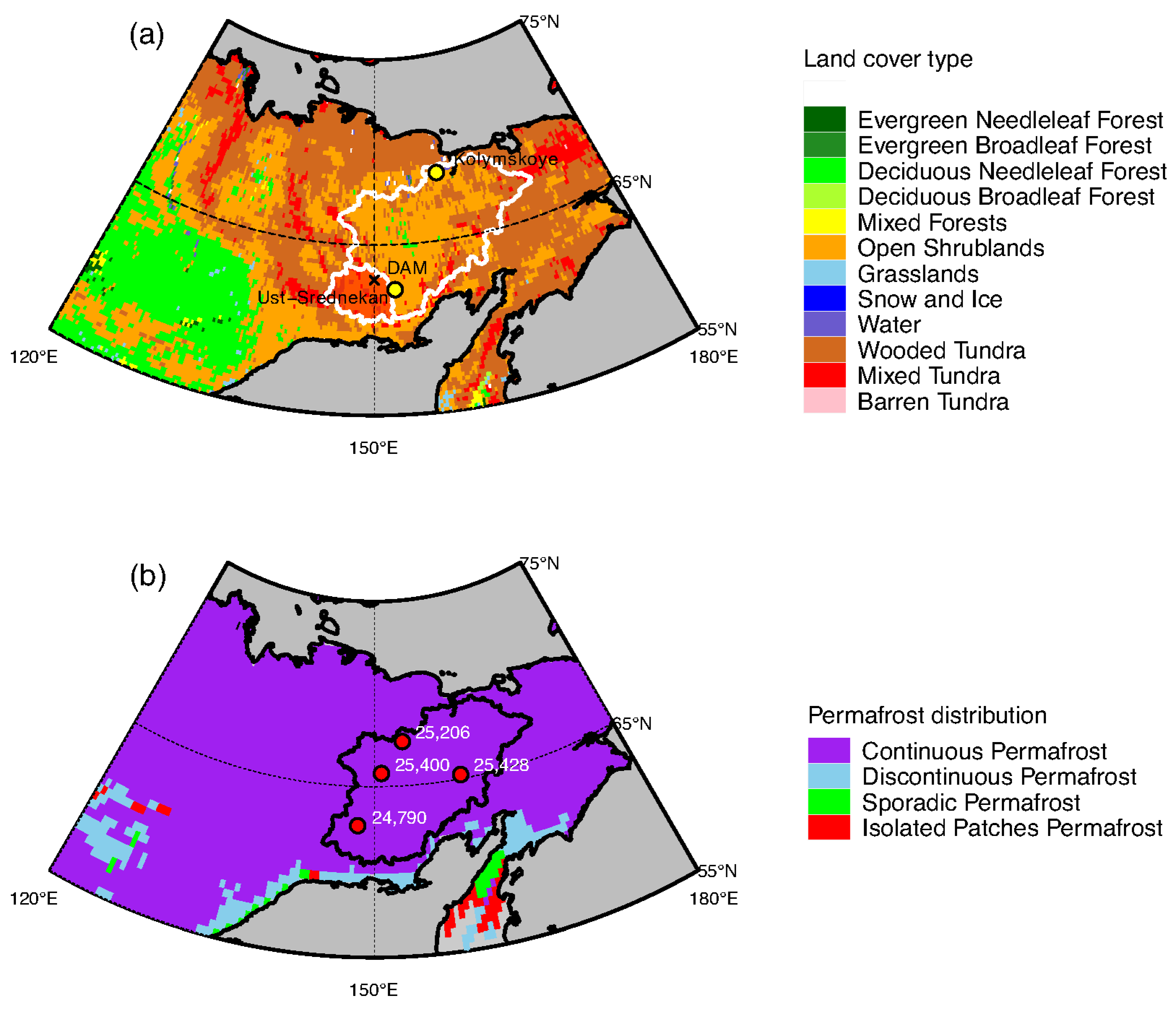
2.1. Study Area

Figure 1a,b show the distributions of the geographical characteristics of the Kolyma River basin, representing the vegetation of the basin boundary and a sub-basin (Dam basin) with a large reservoir (Figure 1a). The vegetation map was obtained from the 1° GLDAS-2/NOAH Dominant Vegetation Type datasets (https://ldas.gsfc.nasa.gov/gldas/GLDASvegetation.php (accessed on 30 July 2021)) using the NOAHv3.3 Vegetation Dataset from GLDAS-2. As shown in Table 1, the Dam basin occupies approximately 15% (99.5 km2) of the total basin area (657.3 km2), and both basins are primarily covered by open shrublands and wooded tundra. Figure 1b shows the distribution of permafrost, based on the data [19]. The Kolyma River basin is entirely covered by continuous permafrost; Figure 1b represents the locations where the soil temperature profiles were measured. Notably, each site had a different length of time series of the observed soil temperature. The available observation durations of sites 24,790, 25,206, 25,400, and 25,428 were from 1979–1989, 1968–2008, 1979–2012, and 1988–1998, respectively.

2.2. Land Surface Model, CHANGE

We used the land surface model, CHANGE (a coupled hydrological and biogeochemical model), which is a state-of-the-art process-based model that calculates heat, water, and carbon fluxes in the atmosphere–land system; the model also calculates soil thermal and hydrological states, including soil freeze–thaw phase changes, stomatal physiology, and photosynthesis. The carbon absorbed through photosynthesis is partitioned into leaf, stem, root, and soil, which are intertwined with land surface processes. The coupling of the dynamic vegetation model in CHANGE facilitates the integration of interactions and feedback in the land system and climate. A remarkable feature of CHANGE is its improved representation of permafrost dynamics achieved through the extension of soil depth to 50.5 m. A zero-heat flux was prescribed as the lower boundary condition. The heat flux into the soil is obtained by solving an energy balance equation, which is considered as the upper boundary condition for the solution of heat conduction. CHANGE numerically solves the heat conduction equation, including the soil water phase changes, to simulate heat conduction between the soil layers. Solving the equation requires soil heat conductivity and capacity, which are determined as the functions of the liquid and ice content and the vertically heterogeneous soil texture [18]. For the simulations, CHANGE required datasets of topography [20], vegetation type [21,22,23], and soil texture [24,25] to show the impacts of land surface on the fluxes. The CHANGE model estimates the ground temperature profile by solving the soil water and heat balance, from which the ALT is obtained. Therefore, in the CHANGE model, permafrost warming could be identified by long-term deepening of the ALT.

2.3. Data

2.3.1. Forcing Meteorological Data

Global Meteorological Forcing Dataset for Land Surface modeling (GMFD)

We used a Global Meteorological Forcing Dataset for land surface modeling (GMFD) with the daily and 0.5° resolutions [26] for model simulations to estimate the terrestrial hydrological cycles and ALT. This dataset has been widely used as a forcing dataset for many land model surface model simulations in the Arctic region [27,28]. The dataset was constructed by combining a suite of global observation-based datasets with the National Centers for Environmental Prediction–National Center for Atmospheric Research reanalysis. Known biases in the reanalysis of precipitation and near-surface meteorology exert an erroneous effect on modeled land surface water and energy budgets, which were therefore corrected using observation-based datasets of precipitation, air temperature, and radiation. Dataset can be downloaded from https://hydrology.princeton.edu/data.pgf.php accessed on 30 July 2021.

University of East Anglia Climatic Research Unit (CRU)

We used the Climatic Research Unit (CRU) climate dataset to verify the surface meteorological datasets of GMFD. The CRU TS4.02 dataset provides homogenized monthly climate data interpolated from over 4000 weather stations and gridded to a spatial resolution of 0.5° [29]. In this study, we used monthly averaged datasets of daily mean air temperature (Ta) and annual precipitation (P). Dataset can be downloaded from http://dx.doi.org/10.5285/b2f81914257c4188b181a4d8b0a46bff accessed on 30 July 2021.

University of Delaware Air Temperature and Precipitation (Udel)

Willmott and Matsuura [30] combined the data from various stations from the Global Historical Climate Network (GHCN) and more extensively, from the archives of Legates and Willmott [31,32]. Udel is a monthly climatology dataset of precipitation and surface air temperature and a time series spanning the period between 1900 and 2015. Dataset can be downloaded from https://psl.noaa.gov/data/gridded/data.UDel_AirT_Precip.html accessed on 30 July 2021.

2.3.2. Satellite Data

Snow Cover Fraction (SCF)

The bimonthly global 0.25° × 0.25° gridded snow fraction over land was generated from satellite-derived bimonthly global snow cover fraction (SCF) product at 0.05° resolution obtained from the JAXA Satellite Monitoring for Environmental Studies (JASMES) website (https://kuroshio.eorc.jaxa.jp/JASMES/index.html accessed on 30 July 2021). The SCF was estimated to be a spatial fraction of snow cover pixels within a 0.25°× 0.25° grid cell. The SCFs were derived from radiance data at different wavelengths, from visible to thermal infrared regions acquired with polar-orbiting satellite-borne optical sensors between November 1978 and December 2019. The SCF of two periods are missing due to poor quality radiance, including the first half of February 1980 to the second half of June 1981 and from the second half of September 1994 to the first half of January 1995. The overall accuracy of snow/non-snow cover classification for the SCF product was estimated to be 0.82–0.99. The detailed analysis and accuracy estimations of the JASMES SCF product were obtained by Hori et al. [33].

Terrestrial Water Storage Anomaly (TWSA)

To quantify the terrestrial water storage anomaly (TWSA) for the study region, we obtained GRACE data (Level-2, Release 5) from three analysis centers: The University of Texas Center for Space Research (CSR), Jet Propulsion Laboratory (JPL), USA, and GeoForschungZentrum Potsdam (GFZ), Germany. We used the ensemble mean of the three GRACE datasets (i.e., simple arithmetic means of CSR, JPL, and GFZ), as recommended by the official GRACE Science Data System, to minimize random errors and enhance common signatures within each GRACE dataset. Additional details about the derivation of the TWSA can be found in Suzuki et al. [34].

2.3.3. Global Land Data Assimilation (GLDAS) System Data (NOAH)

The GLDAS version 2.0 (GLDAS-2) [35], which currently uses only the NOAH land surface model and the GMFD meteorological forcing dataset as the only source of forcing data, was corrected using observation-based inputs of precipitation, surface air temperature, and radiation. GLDAS-2 was verified to estimate the TWSAs and terrestrial hydrological processes in Siberia [35,36] against the GRACE-based TWSA. Thus, we used GLDAS-2 as a reference for the CHANGE simulations. However, GLDAS-2 does not estimate ALT and permafrost dynamics because it can only consider a soil-layer depth of 2 m. Thus, hereafter, we refer to this model as NOAH, which is used for comparison with the CHANGE model.

2.3.4. River Flow Rate Data

The measured flow rates at the lowest hydrological stations of the Kolyma River were used to analyze basin-scale variations in the river discharge. We used discharge data from the Arctic Great Rivers Observatory (ArticGRO) [37] Discharge Dataset Version 20,180,713 (https://www.arcticrivers.org/data accessed on 30 July 2021) [38]. Discharge data were obtained from two gauge stations: the Kolymskoye (1978–2008) (68.73°N, 158.72°E) and the Kolymsk-1 (2009–2016) (68.73°N, 158.72°E) stations in the Kolyma River. In addition, river flow from the Dam basin was observed at Ust-Srednekan, which is located in the uppermost basin of the Kolyma River. The river flow in Ust-Srednekan from 1979 to 2012 was obtained from the monthly Meteorological Bulletin of the Russian Hydrometeorological Service [39].

2.3.5. Soil Temperature Data

The database of monthly soil temperature under natural land cover at different depths down to 320 cm from four weather stations of the Kolyma River Basin over a period of 1968–2012 was compiled from different sources. We averaged the daily soil temperature to obtain the monthly values for the period from 1979 to 2012 based on the dataset of the All-Russia Research Institute of Hydrometeorological Information World Data Center (freely available at http://meteo.ru accessed on 30 July 2021). A detailed description about the soil temperature datasets and their quality control methods can be found in the study conducted by Sherstyukov and Sherstyukov [40]. Historical data with some missing records during 1969–2012 was obtained from the monthly Meteorological Bulletin of the Russian Hydrometeorological Service [39,41]. Within the Kolyma River basin, we selected four observation sites, namely station ID 24,790, 25,206, 25,400, and 25,428, because these sites provided more than 20 years of continuous monthly data without a gap in the summer. The available observation period for each site was 27 years (1985–2012) for site 24,790, 25 years (1979–2004) for site 25,206, 33 years (1979–2012) for site 25,400, and 24 years (1988–2012) for site 25,428. In many cases, the data from these four sites were also absent during winter months, and there were years when observations were available only during the summer months.

2.4. Theory

To calculate the monthly TWS using the CHANGE and NOAH data, we applied the water balance equation proposed by Suzuki et al. [14], expressed as follows:
TWSA = SWEA + CSA + SMA + GWA + SWA
where SWEA is the snow water equivalent anomaly (mm/month), CSA is the anomaly of the total amount of water within the canopy (mm/month), SMA is the anomaly of vertical accumulated soil moisture within the total soil layer (mm/month), GWA is the change in groundwater or ice over the permafrost (mm/month), and SWA is the anomaly of surface water bodies (such as lakes, river water, and wetlands; mm/month).
As CWA is a minor factor and GWA was not available, the TWSA determined from the land surface model depended primarily on SWEA and SMA.
The subgrid-scale model-based SCF was determined as a function of the SWE [42]:
SCF = 1 e x p 2.6 SWE SWE max SWE SWE max e x p 2.6
where SWE is snow water equivalent and SWEmax is the vegetation-dependent maximum snow water equivalent; SWEmax was set as 40 mm. Notably, when SWE is greater than SWEmax, the SCF is equal to 1.

2.5. Analysis

2.5.1. Statistical Analysis

We conducted statistical analyses using nonparametric methods based on the approach of Ichii et al. [43]. These statistical techniques do not require the assumption of normality in variance and are more robust against anomalous outliers. The slopes of the trends were calculated based on the Theil–Sen slope (hereafter referred to as Sen’s slope). We used the Mann–Kendall (MK) trend test to assess the significance of the trend. All correlation analyses were based on the Spearman correlation coefficients (R). Notably, all statistical tests applied in this study had a significance level of p < 0.05.
The lag correlation analysis of the terrestrial hydrological elements in the permafrost zone was performed using the relationships between the annual mean TWSA of a given year and the annual precipitation or evapotranspiration of the same year, or three years before or after. Correlation coefficients were calculated using R, and lag correlations were considered significant at p-value of <0.05.

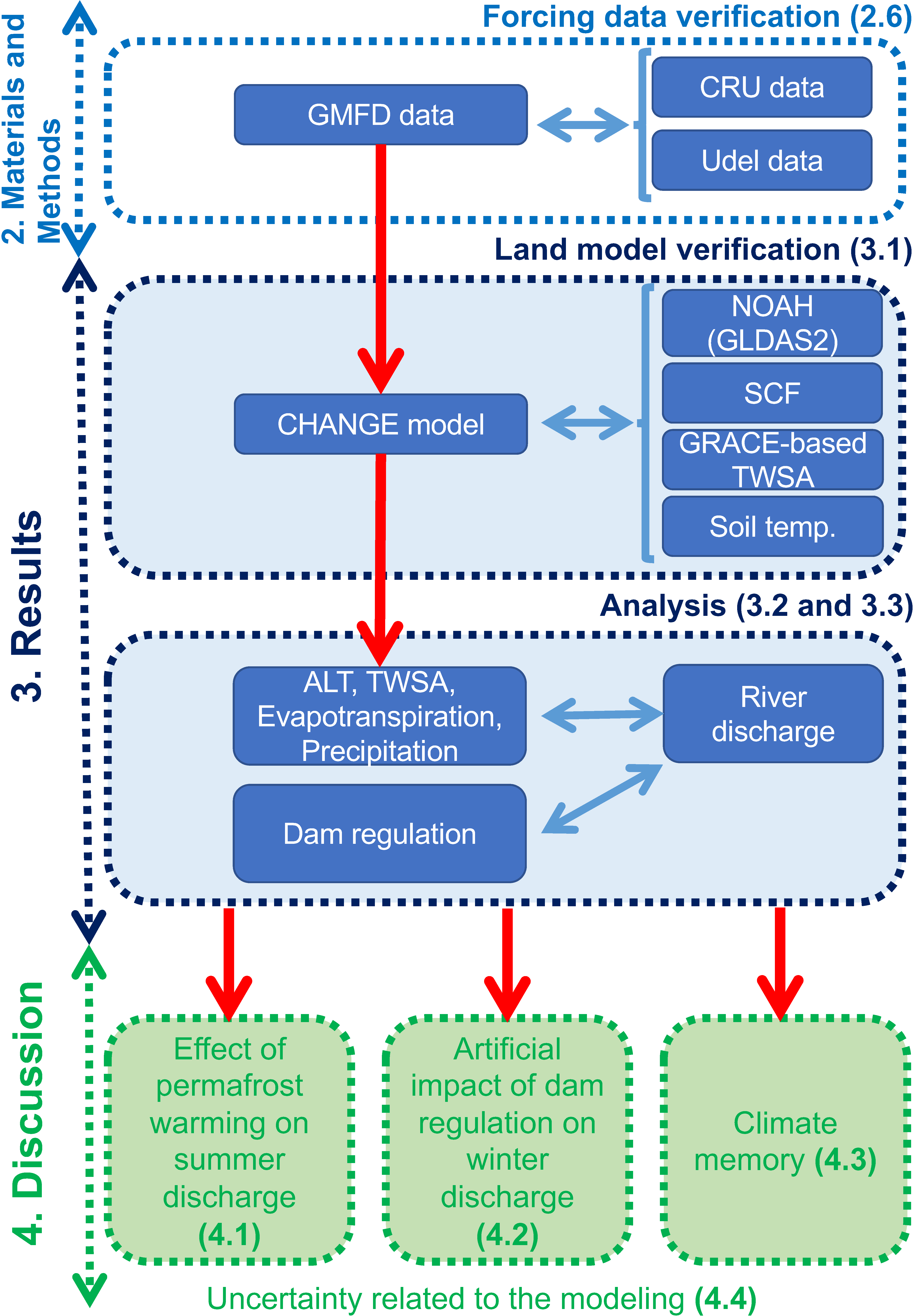
2.5.2. Analysis Flow

Figure 2 illustrates the analysis flow in this study. Section 2.6 discusses the verification of forcing variables, and Section 3.1 provides the CHANGE model performance against NOAH model, SCF, GRACE-based TWSA, and in situ soil temperature profiles. Section 3.2 explains the seasonal variations in hydrometeorological conditions in the whole Kolyma River basin, and Section 3.3 discusses the hydrological changes. Finally, we discuss the effect of permafrost warming on summer discharge in Section 4.1, the artificial impact of dam regulation on winter discharge in Section 4.2, climate memory in Section 4.3, and uncertainty related to the modeling in Section 4.4.

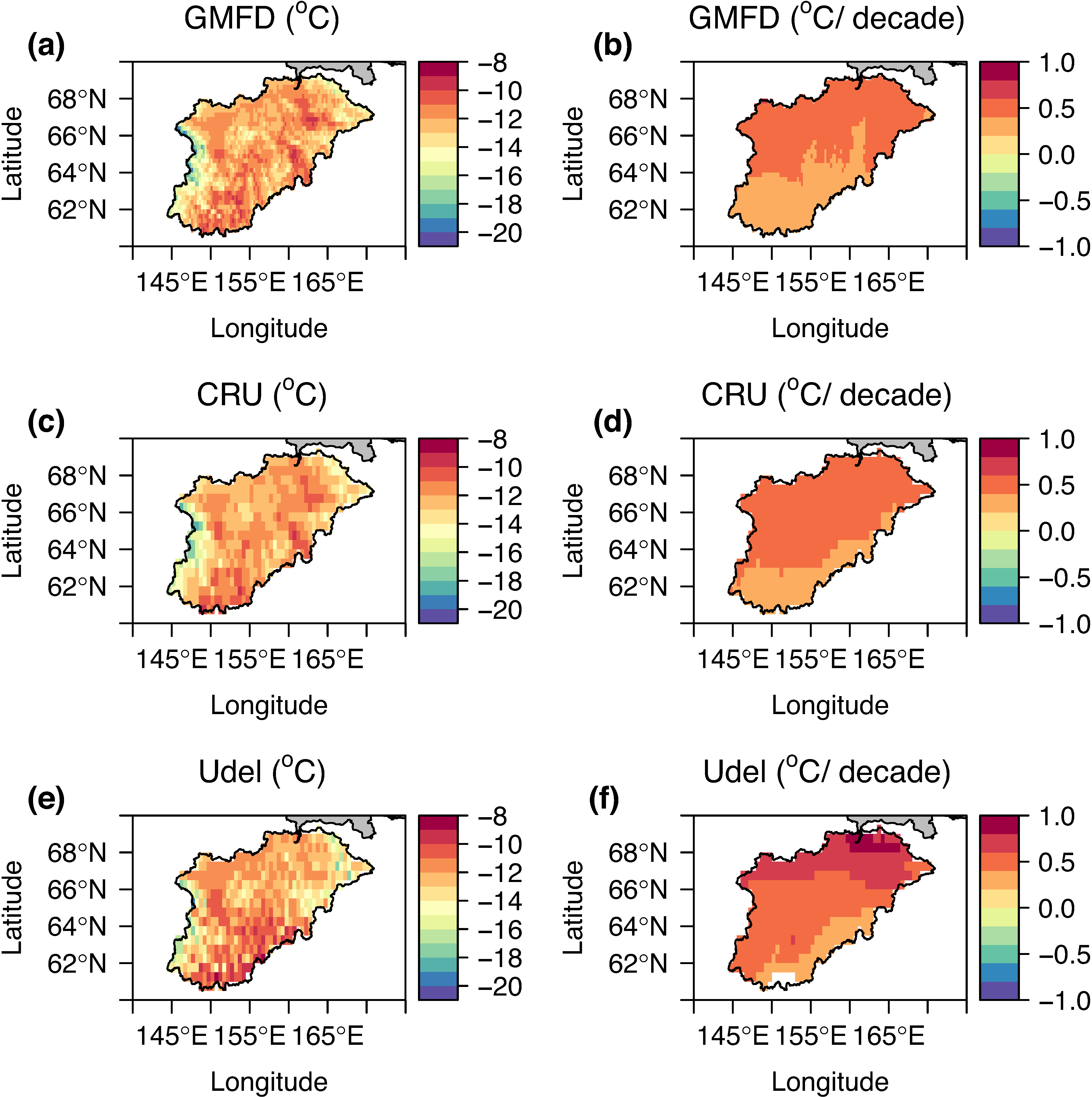
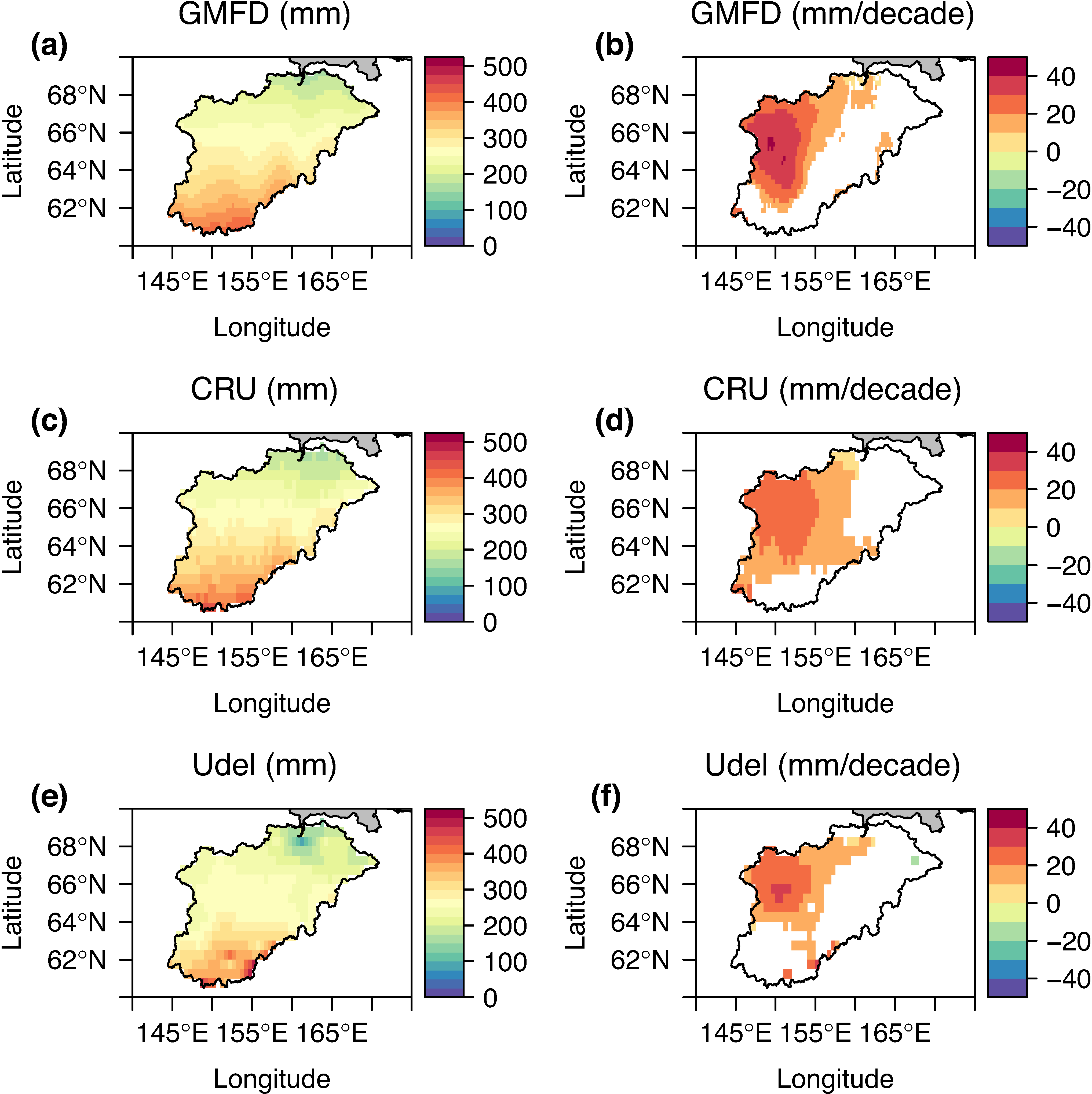
2.6. Verification of Forcing Variables

To confirm the reliability of the GMFD forcing data, we compared it against two similar global datasets: CRU and Udel. First, we determined the climatological air temperature data from the three datasets. Figure 3 shows the climatology and trend in annual mean Ta for the three different forcing datasets used in our study. Figure 3a,c,e show the climatology of the annual mean Ta by GMFD, CRU, and Udel, respectively, recorded during a 34-year period (1979–2012). The three datasets exhibited very similar spatial patterns and magnitudes. Figure 3b,d,f show linear trends in the annual Ta from 1979 to 2012. There were latitudinal gradients among all three trends; the northern part of the Kolyma River basin exhibited a greater warming trend than the southern part. The magnitude of the warming trend in the northern area was over 0.5 °C/decade, whereas the southern part exhibited a magnitude <0.2 °C/decade. The warming in the Udel datasets was stronger than the other two datasets; however, the regional warming trend in air temperature among the three datasets was very similar. Thus, Ta for the GMFD data was compatible with those of the other two datasets (CRU and Udel).
In addition to Ta, precipitation is important for determining the river discharge and hydrological cycle. Figure 4 shows the climatology and trend in the annual precipitation for the three different forcing datasets from 1979 to 2012. Figure 4a,c,e show the spatial variations in annual precipitation for the 34-year period obtained from the GMFD, CRU, and Udel datasets, respectively. All datasets exhibited very similar latitudinal gradients in terms of precipitation. Figure 4b,d,f show linear trends of annual precipitation from 1979 to 2012. There were longitudinal gradients among the trends of the three datasets; a higher increasing trend could be observed in the western part recording more than 10 mm/decade; however, the eastern part did not exhibit statistical significance. The spatial pattern of precipitation trends was similar among the three datasets. Notably, the magnitude of the increasing precipitation trend in the western area was more than 10 mm/decade. Although the increasing precipitation in the GMFD dataset was stronger than that in the other two datasets, the regional increasing trend of precipitation in all the three datasets was evidently similar. Thus, the annual precipitation in the GMFD data was compatible with those of the other two datasets (CRU and Udel).

3. Results

3.1. Model Performance

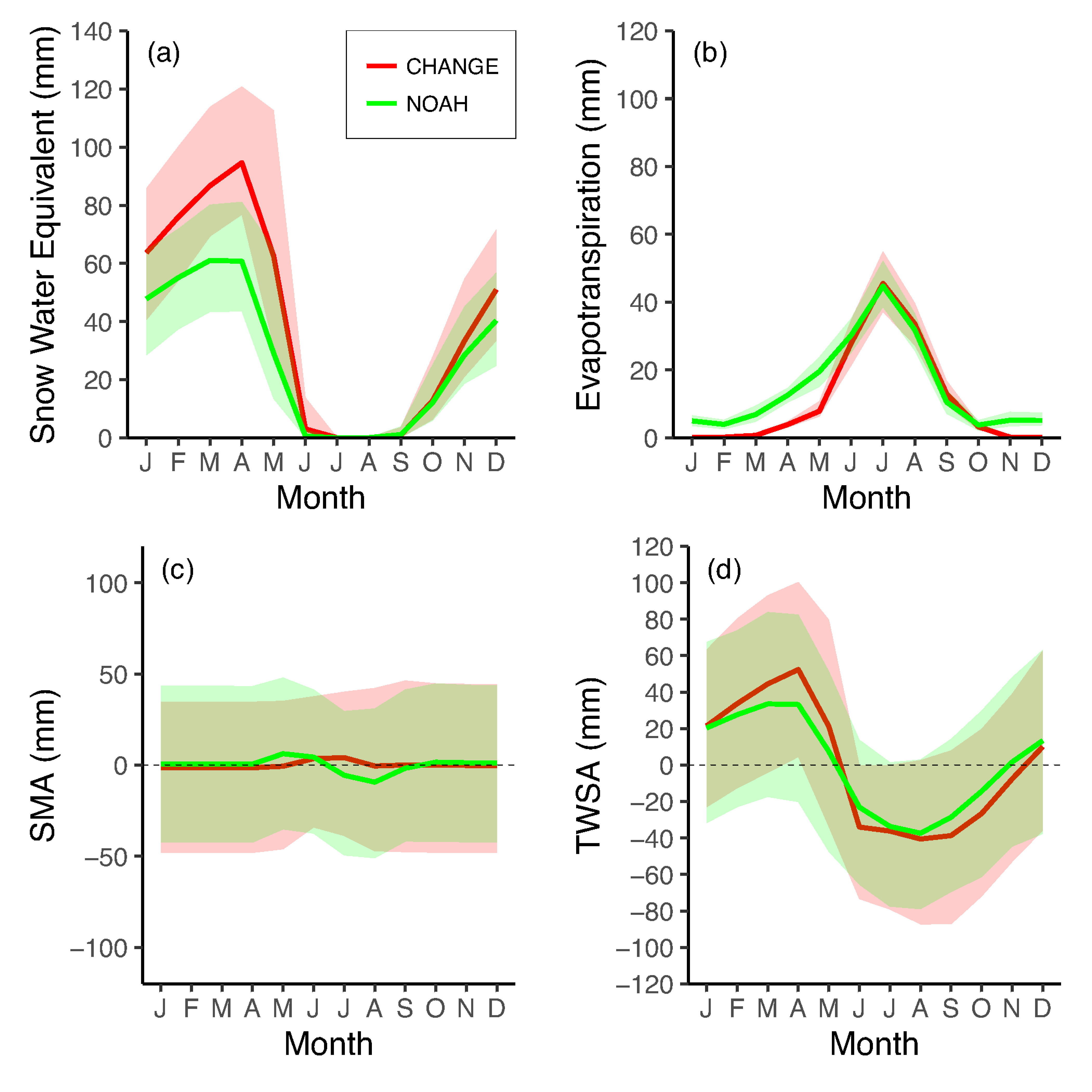
3.1.1. Global Land Data Assimilation (NOAH) vs. CHANGE

First, we compared the simulated terrestrial water balance components between the CHANGE and NOAH models. NOAH-based TWSA products are used in TWSA evaluations using GRACE-based TWSA [33]. Figure 5 shows the seasonal variations in monthly climatology in the hydrometeorological variables derived from the CHANGE and NOAH model simulations during 1979–2012. The shaded area denotes the 95% confidence interval (CI). According to Figure 5a, the SWE of the CHANGE model is higher than that of the NOAH model. This is because winter sublimation is higher in the NOAH model than in the CHANGE model (Figure 5b). Monthly winter sublimation by NOAH remained stable at 5 mm, whereas the CHANGE-simulated sublimation was significantly smaller in spring and approximately zero across the winter season. Thus, the SWE estimation can be very sensitive to the winter sublimation estimation revealed by Suzuki et al. [44]. However, we cannot assess which model is better because of the lack of validated data on winter sublimation or SWE in the Kolyma River basin. In Figure 5c, the soil moisture anomaly (SMA) obtained from both models varied from year to year, and the monthly climatological mean SMA was approximately zero for CHANGE and NOAH. Seasonal changes derived from both models were different, with seasonal variations corresponding to TWSA, and more stable SMA obtained using CHANGE. Finally, the TWSA obtained by both models had very similar seasonal variations, with similar CIs.

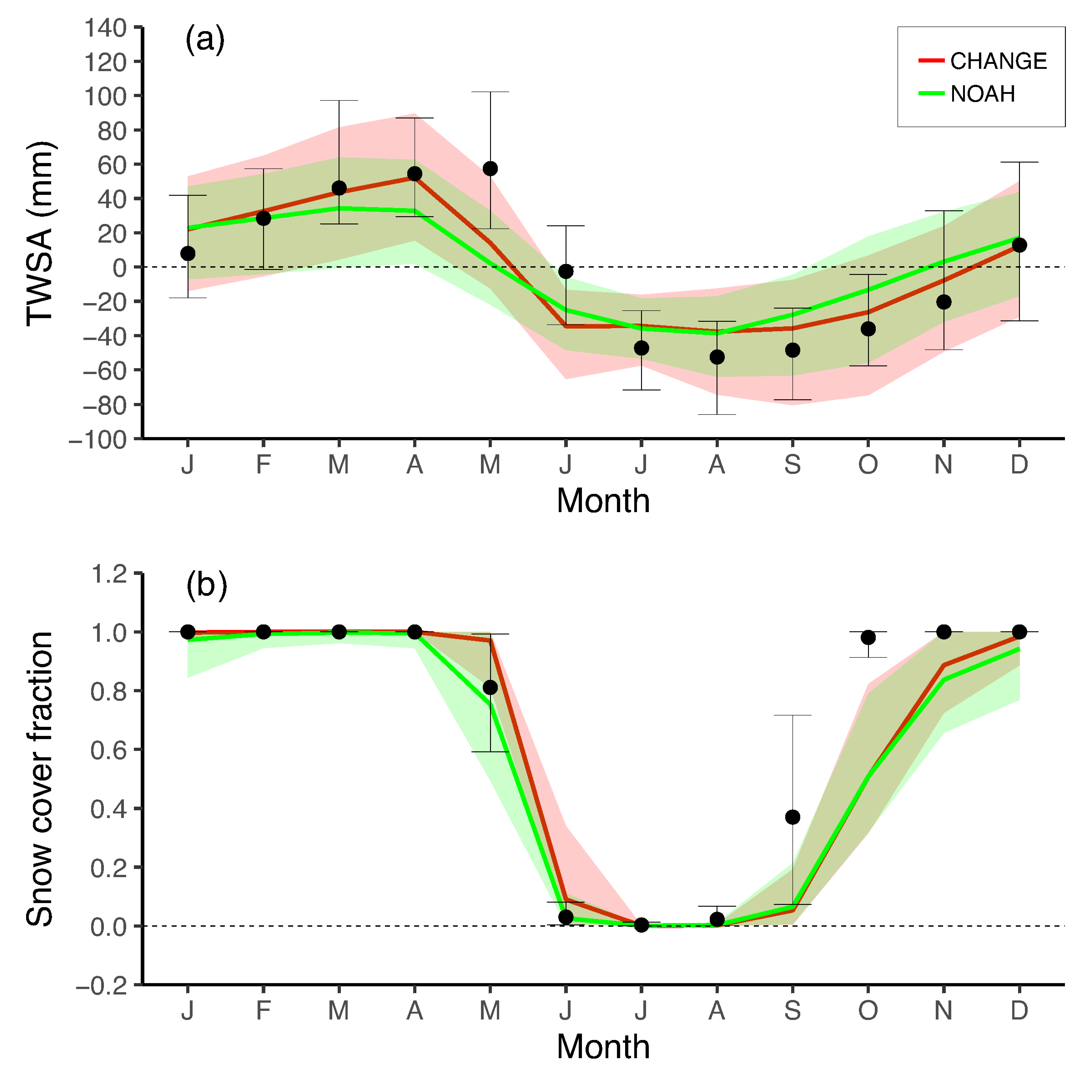
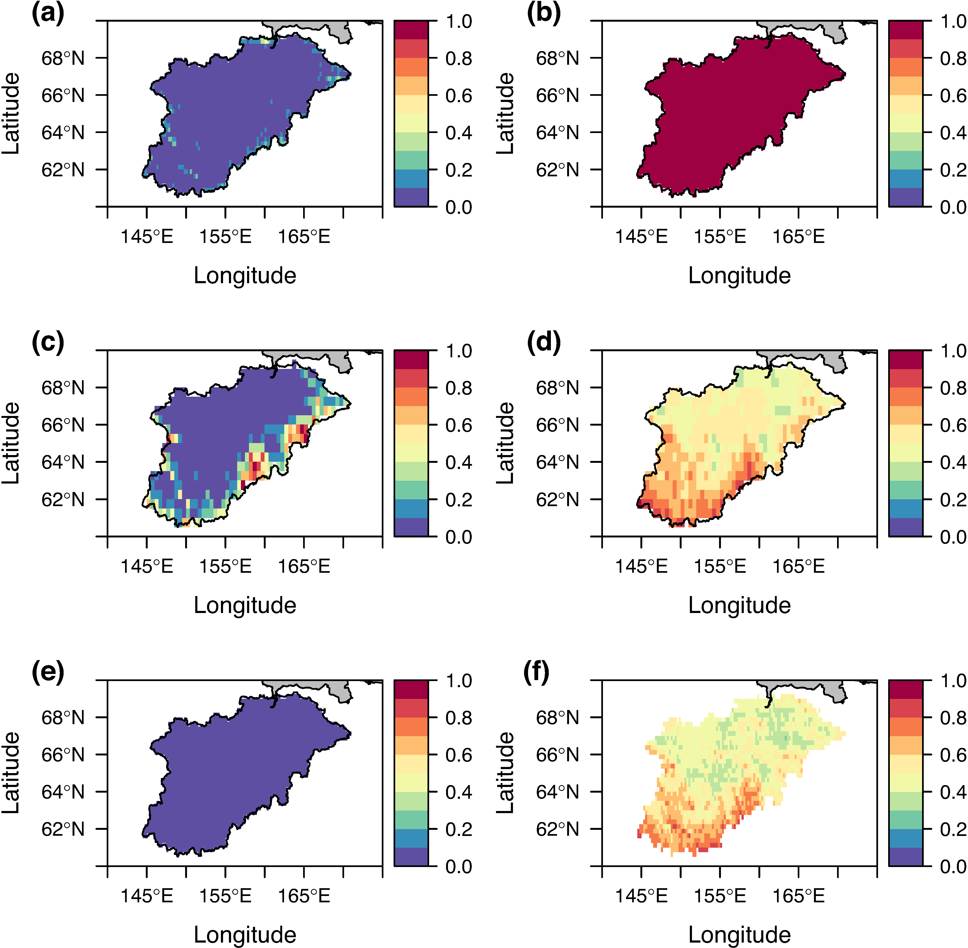
3.1.2. Verification against Satellite-Based Products

Figure 6a shows a comparison of the seasonal TWSA estimated by the CHANGE and NOAH models. The CHANGE and NOAH models reproduced similar seasonal changes with the GRACE-based TWSA. The most significant difference in TWSA between the satellite and models was observed in May; the highest TWSA value was recorded by the GRACE observation, whereas the underestimations in the CHANGE and the NOAH models were caused by snowmelt runoff from inside to outside the basin. One of the reasons for this is that the model does not adequately represent the fact that most of the snowmelt water is temporarily retained in the basin via wetlands, rather than flowing immediately into the basin river. Table 2 presents the performance of both models in terms of statistics, namely root mean square error (RMSE) and Nash–Sutcliffe efficiency (NSE), suggesting that CHANGE is better than NOAH with respect to TWSA estimation.
The CHANGE and NOAH models efficiently reproduced the basin-averaged SCF (Figure 6b). However, compared to the SCF during the snowmelt season, the model lags the observed satellite SCF during autumn. This may be attributed to the fact that the original horizontal resolution of the satellite was 5 km, whereas the model’s horizontal resolution was approximately 50 km at 0.5°, that is, approximately 10 times coarser in horizontal resolution. Due to the coarse topography in the model, the subgrid-scale snow distribution could not be adequately represented, particularly in autumn when snow initiation resulted in the largest heterogeneous snow cover (compared with that in spring) [45].
To comprehensively compare the reproducibility of the SCF, we assessed the 34-year average SCF during the months of June and October using satellite data and model estimates. As snowing initiates and finishes in June and October, respectively, the SCF in the basin mostly fluctuates. Thus, the two months are considered suitable for model validation. Figure 7a–f shows the spatial distributions of SCF from satellite data and two different model simulations (NOAH and CHANGE). For the June SCF, the results from CHANGE were slightly larger than satellite observations; however, the NOAH-simulated results were almost similar to the satellite observations (Figure 7c,e). Thus, the CHANGE model tended to show delays in snowmelt in mountainous areas with high elevation. Meanwhile, in October, the model had lower SCF throughout the basin than the satellite observation that had entirely the unity value. In October, although there was no significant difference between the CHANGE and NOAH models, the CHANGE model exhibited a slightly high SCF (Figure 7d,f).

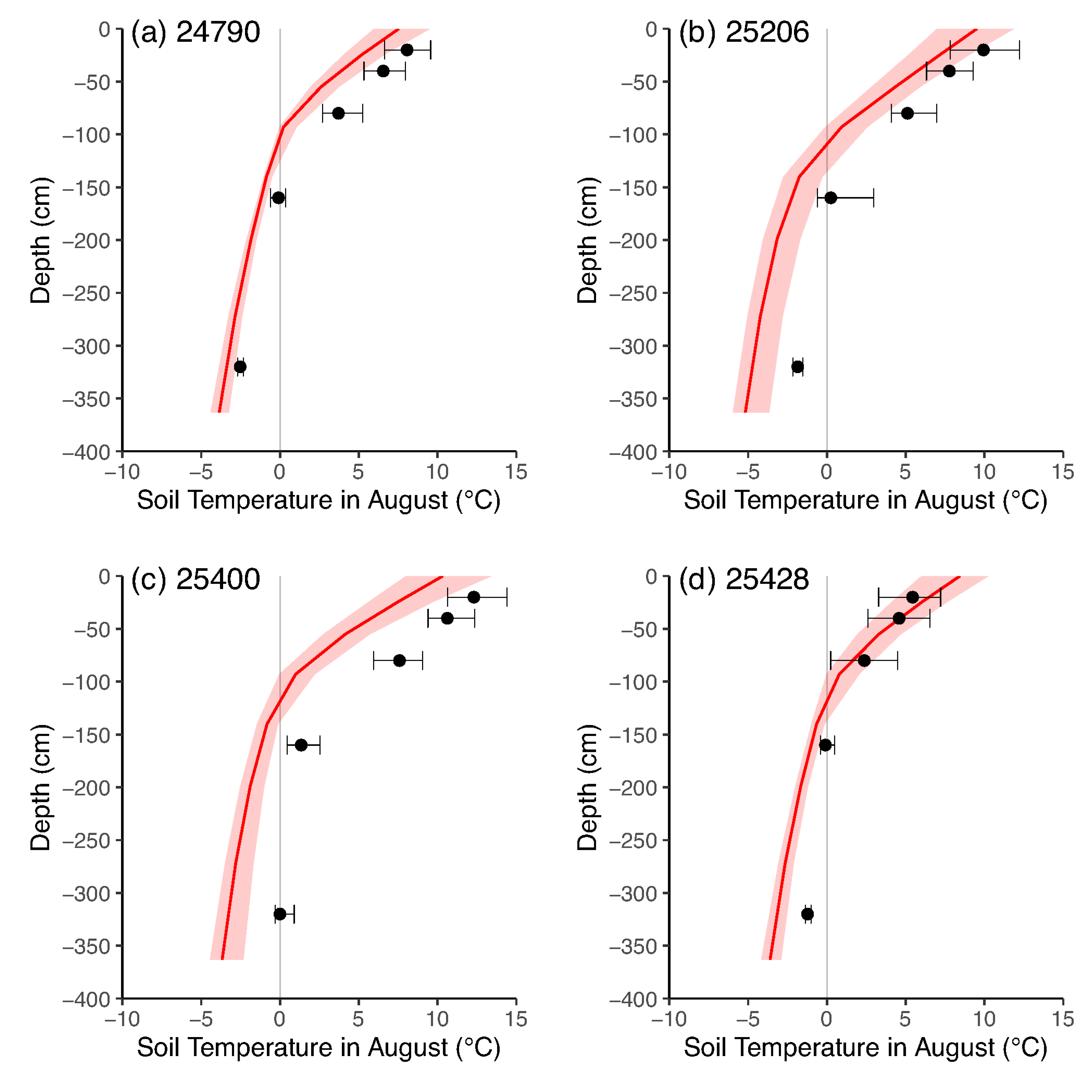
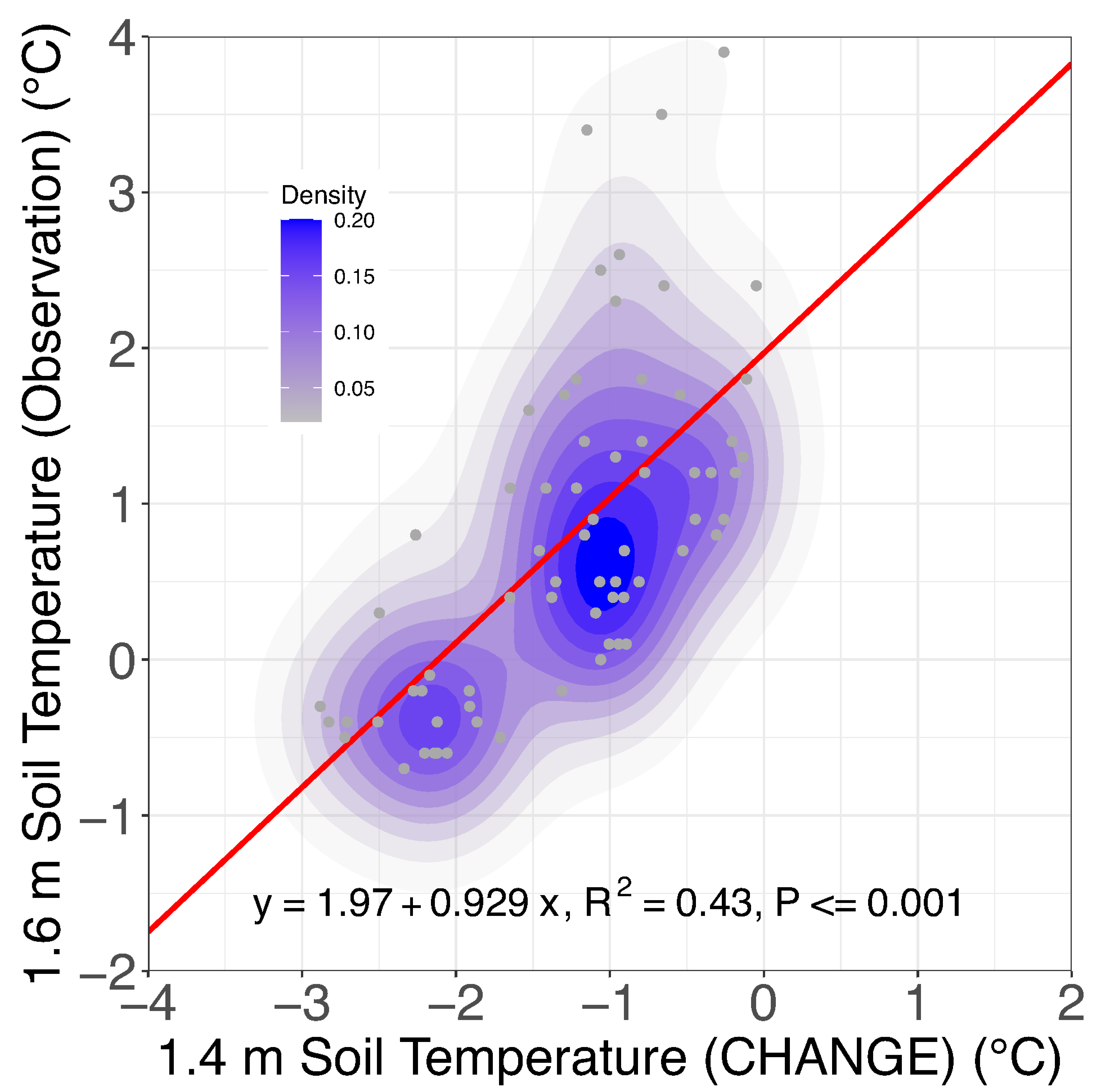
3.1.3. Comparison of Soil Temperature

To evaluate the performance of the model against in situ soil temperature data, we compared the observed ground temperature with the CHANGE estimate because NOAH does not incorporate permafrost into the model; only the performance of the CHANGE model is shown here.
Figure 8 shows vertical profiles of soil temperature climatology in August at four meteorological stations in the Kolyma River basin; the soil temperature in August had the longest records. CHANGE-simulated soil temperature profile climatology was similar to the observed profile climatology in all sites. However, the simulated soil temperature was lower than the observed one because weather stations that observed soil temperature were artificially deforested to observe the meteorological conditions in open fields. According to Goncharova et al. [46], this artificial condition can increase soil temperature and permafrost degradation. However, the CHANGE model considered the shrub vegetation in the Kolyma basin, where the vegetation cover directly intercepts solar radiation, consequently indicating a lower soil temperature. Thus, we assumed that the discrepancy in soil temperature between the observation and simulation is attributable to the different land covers. The similarity in the observed and simulated soil temperature profiles suggests that the energy balance within the subsurface can be efficiently reproduced by the CHANGE model.
Figure 9 shows how the CHANGE model can estimate the interannual variations in subsurface temperature. We compared the observed soil temperature (at 1.6 m depth) and CHANGE-simulated soil temperature (at 1.4 m depth) in August at sites 24,790, 25,206, 25,400, and 25,428 (Figure 9), where the ground temperature was observed (because the model does not calculate the ground temperature at 1.6 m). We observed a strong linear relationship between the observation and the simulation. Thus, we can confirm that CHANGE could effectively reproduce the interannual variations in the soil temperature for the Kolyma River basin. In addition, the active layer depth was closely related to the soil temperature profile. Therefore, the CHANGE model can be expected to reproduce ALT for the study area.

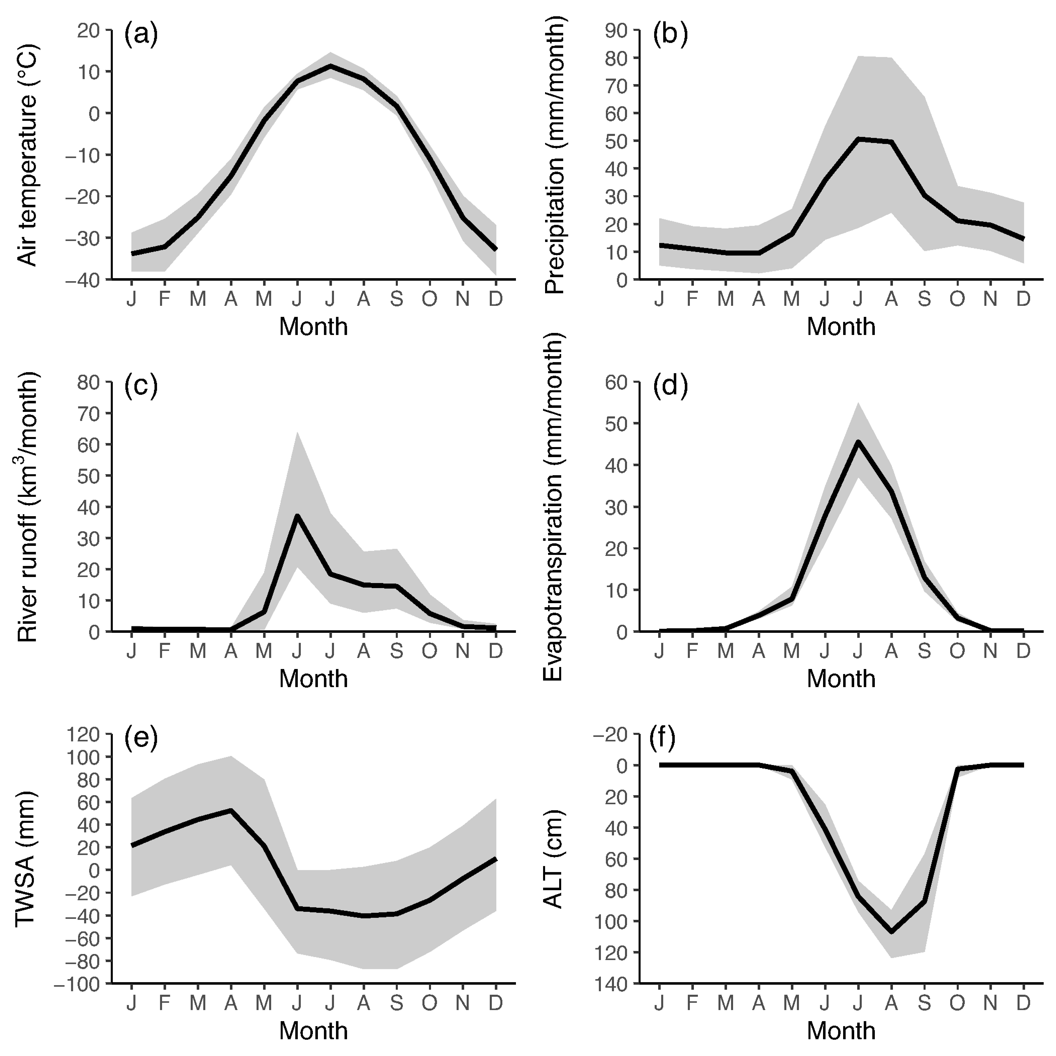
3.2. Seasonal Variations in Hydrometeorological Conditions

We revealed the characteristics of seasonal variations in the basin-averaged monthly hydrometeorological components in the Kolyma River basin. Figure 10a–f shows the basin-averaged climatology of the seasonal variations in the hydrometeorological variables from 1979 to 2012. The minimum monthly temperature reached −35 °C in January, whereas the maximum monthly air temperature reached 10 °C in July. The interannual monthly temperature variation in winter was larger than that in summer, as shown in Figure 10a for the 95% CIs (gray shaded area). Figure 10b shows that most of the precipitation occurred in the summer, from June to September. Corresponding to the higher summer precipitation along with snowmelt water, we could deduce that the river runoff from the mouth of the Kolyma River basin was dominant, and the interannual variability of the river runoff was the largest as shown with 95% CIs (gray shaded area in Figure 10c). The major river runoff was observed from June to September (Figure 10c). The major CHANGE-simulated evapotranspiration also occurred from June to August (Figure 10d). However, the interannual variation in evapotranspiration can be smaller than that in precipitation and river runoff. As shown in Figure 10e, TWSA in the Kolyma River basin is predominantly controlled by snow mass variations over the basin, with large interannual variations (gray shaded area of Figure 10e). The ALT increased in June and reached a maximum in August (Figure 10f). From September through October, the ALT decreased and reached zero in October over the winter season. The maximum basin-averaged ALT in August was approximately 1 m.

3.3. Hydrological Changes

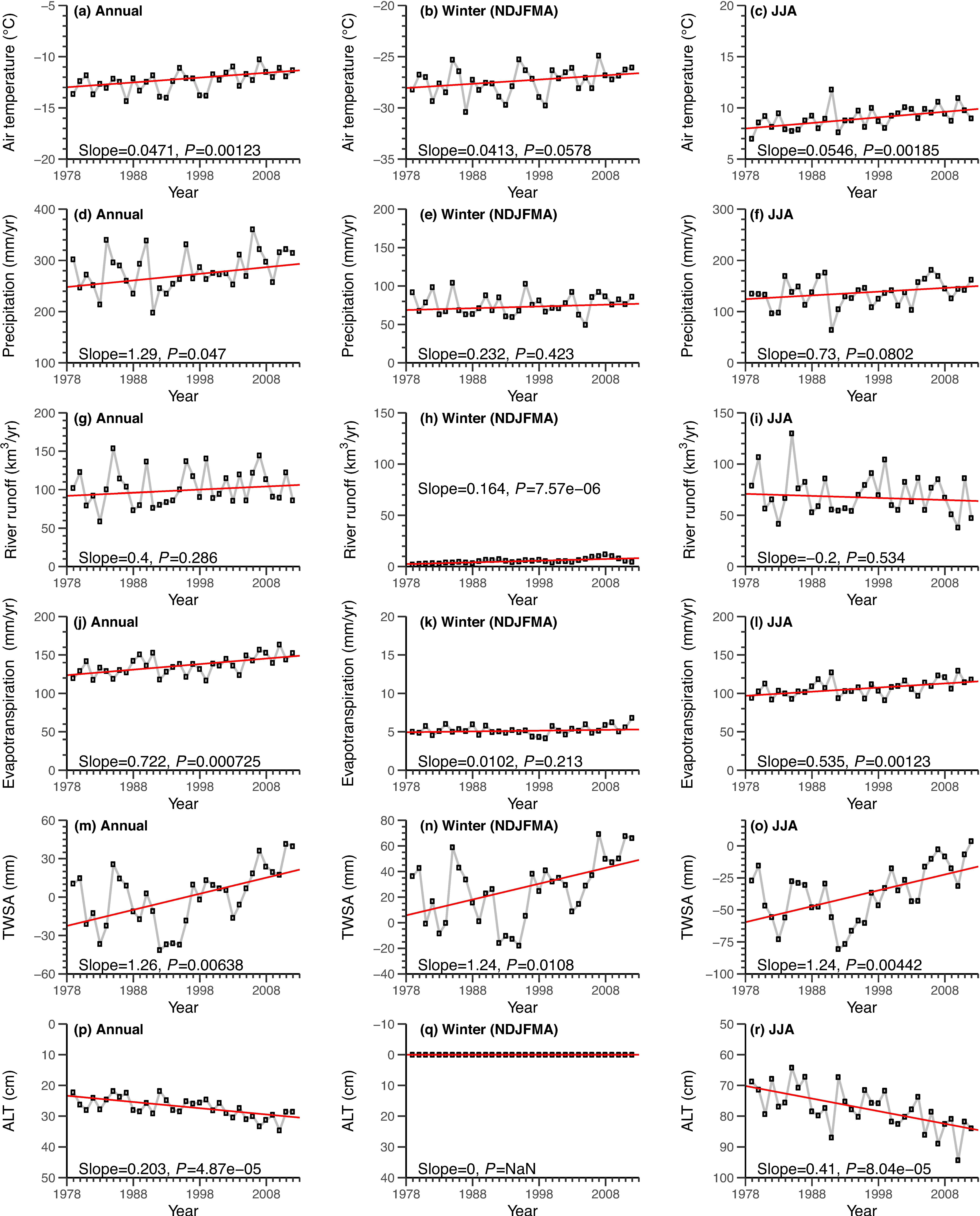
3.3.1. Interannual Variability

In this section, we present the interannual variations in river discharge and related hydrometeorological factors in the Kolyma River basin. In terms of the annual variations, winter (November to April, NDJFMA) and summer (June to August, JJA) air temperatures in the Kolyma River basin exhibited an evident increasing trend (Figure 11a–c). Thus, the Kolyma River basin has been significantly affected by the warming air temperature. The warming trend was slightly stronger in summer than in winter. Similarly, annual and summer precipitation exhibited a positive trend, and the increase in winter precipitation was not significant (Figure 11d–f). Overall, in the Kolyma River basin, the changes in air temperature and precipitation were more significant in summer than in winter. Regarding the river discharge at the outlet of the Kolyma River basin, an evident increasing trend was observed during winter, and the annual river discharge exhibited a small increasing trend (Figure 11g,h). Although summer warming and precipitation increase were identified in our analysis (Figure 11c–f), Figure 11i shows a slight decrease in the summer river runoff (statistically insignificant). This opposite trend observed in summer precipitation and river runoff will be discussed later.
Figure 11j–l shows the annual, winter, and summer evapotranspiration over the basin. A significant increasing trend of evapotranspiration was observed annually and in summer; evapotranspiration was very small during winter and exhibited no significant trend. Except for winter, this increasing trend of evapotranspiration corresponded to the warming trend. TWSA of the Kolyma River basin was calculated using the estimated terrestrial water balance. With respect to the TWSA trend, the changes in the annual, winter, and summer averaged TWS for the basin are shown in Figure 11m–o; these figures show an evident increasing TWS trend, indicating that the water storage trend in the basin increased during the study period. The annual and summer averaged ALT exhibited an evident increasing trend (Figure 11p–r). The summer mean ALT increased approximately 15 cm during the study period, and the yearly average ALT increased 7 cm during the same period. Based on the above ALT trends, we can conclude that the upper parts of permafrost have shifted to the warming phase.

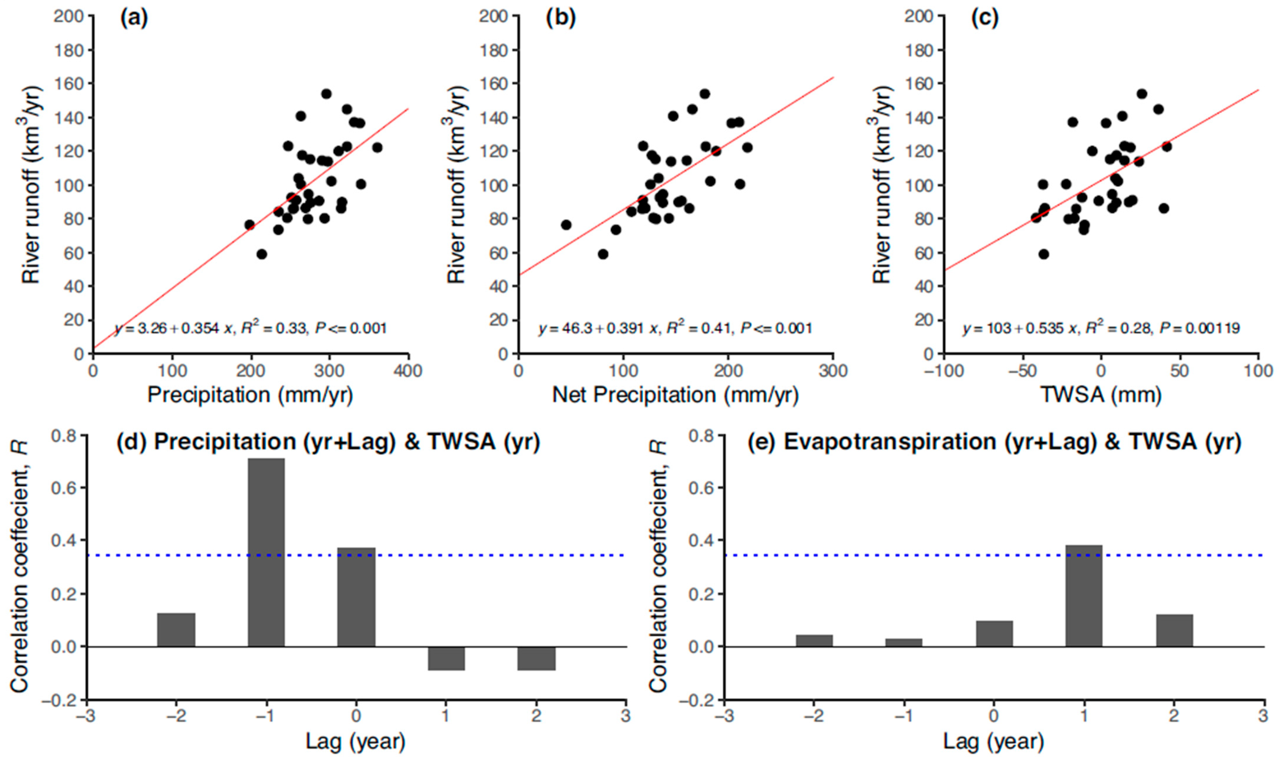
3.3.2. Correlation Analysis

We deduced the relationship between the observed annual river runoff and its related components. Figure 12 shows the relationship between the annual river runoff and precipitation (a), net precipitation (P-E) (b), and TWSA (c). In this analysis, we used CHANGE-simulated evapotranspiration and TWSA values. The figures indicate that the three components have a significant positive correlation with the annual river runoff (Figure 12a–c). In particular, the correlation coefficient between river runoff and precipitation was high (Figure 12a), and the regression slope between river runoff and net precipitation (precipitation minus evapotranspiration) was considerably higher (Figure 12b). Therefore, evapotranspiration is an important factor causing the interannual variations in river runoff. In addition, annual river discharge was largely controlled by TWSA (Figure 12c), as reported previously [34].
We also deduced the correlation among TWSA and hydrological parameters. Figure 12d,e show the lag correlation coefficients (R) between the TWSA and precipitation and evapotranspiration, respectively. The lag year was used for deducing the correlation of precipitation and evapotranspiration against the year of the TWSA. Negative and positive lags imply that the lag years advanced and delayed from the target year of the TWSA, respectively. We found a significant lag correlation. The lag correlation indicates that the TWSA is largely dependent on the precipitation of the previous year. The relationship between the TWSA and the lagged evapotranspiration after one year also exhibited a statistically significant and positive correlation (Figure 12e).
Overall, the precipitation is trapped in a shallow active layer, which determines the TWSA in the following year. Additionally, evapotranspiration increases one year after the TWSA increases. The TWSA and river runoff had no lag and had a highly significant correlation in the same year. Thus, TWSA controls river discharge and evapotranspiration.

3.3.3. Seasonal Discharge

Winter Discharge

We examined the effects of anthropogenic activities (i.e., dam regulation) on the discharge during winter. Majhi and Yang [8] reported that winter discharge in the Kolyma River basin is strongly influenced by dam regulation that began in 1987 in the Kolyma River basin. Thus, we set the pre-dam period as 1979–1986 and the post-dam period as 1987–2012. To understand the impact of dams on the annual and winter river discharges, we analyzed the river discharge between the pre-dam (1979–1986) and post-dam (1987–2012) periods.
Figure 13a–c shows the comparison of discharge from the total basin and the Dam basin in the annual and winter seasons for individually different periods. According to these results, the increase in winter discharge in the entire basin after the construction of the dam corresponded to an increase in the discharge in the tributaries of the dam, consistent with the results of Majhi and Yang [8]. The increase in the winter discharge of the Kolyma River is primarily due to the effect of dam operation. However, the annual discharge of the entire basin did not vary significantly before and after the dam construction. This can be attributed to the very low discharge during winter and the fact that the dam tributary area only accounts for approximately 15% of the total basin. Therefore, the effect of the dam can be ignored when considering the variations in the annual and summer river runoffs.

Summer Discharge

Summer discharge is a dominant component of the annual discharge. In this study, we deduced how summer discharge can be affected by permafrost dynamics. Figure 11f,i show a significant increasing trend in precipitation but a small decreasing trend in the river discharge; despite the increase in precipitation, the discharge decreased. Figure 14a shows the relationship between the summer discharge and JJA mean ALT after removing their linear trends between 1979 and 2012. An evident decrease in the summer runoff was observed as the active layer is thicker, implying that the summer river runoff decreases when the JJA mean ALT increases. Figure 14b shows the relationship between the sum of the JJA mean TWSA and evapotranspiration and JJA mean ALT, clearly indicating that the thicker the active layer (the more the permafrost thaws), the larger the sum of TWSA and evapotranspiration in summer. This implies that as ALT deepens, it reduces river discharge but increases evapotranspiration and TWSA. This is possibly because an increase in ALT will increase the storage; therefore, when precipitation increases, it will be first stored in the storage tank. The increase in storage will eventually lead to an increase in TWSA, which in turn will increase ET as it reduces soil moisture stress.

4. Discussion

4.1. Effect of Permafrost Warming on Summer Discharge

The effect of permafrost thawing will be discussed for the summer discharge. Walvoord and Kurylyk [47] revealed that continuous permafrost prevents water infiltration into deeper soil layers, while a part of the subsurface water in the discontinuous permafrost region is associated with groundwater, which likely increases subsurface flow. They also demonstrated how the changing permafrost affects water movement, suggesting that as the ALT increases, the storage volume of the land increases.
Biskaborn et al. [48] examined the permafrost temperature at a depth of approximately 10 m and revealed that ground temperature in the Siberian region has been rapidly increasing in recent years. Figure 15 shows the temporal variation in the observed annual mean soil temperature at site 25,206 from 1969 to 2008. The ground temperature has been warming rapidly since mid-1990s, and the ALT was recorded as 1.6 m in 2003. As shown in Figure 11i, the summer river flow of the Kolyma River has been decreasing rapidly since mid-1990s. The observed rapid increase in the ground temperature and the significant decrease in the summer river flow of the Kolyma River has occurred almost synchronously since mid-1990s. This suggests that deep soil warming is associated with the recent summer discharge decrease. This result is consistent with the CHANGE-simulated result as ALT has been rapidly increasing since the mid-1990s along with TWSA (Figure 11o,r). In addition, the increase in TWSA due to deeper ALT may have reduced soil moisture stress, resulting in increased evapotranspiration. These results correspond to previous findings [49]. The above results suggest that the decreased trend in summer river runoff was caused by the increase in both water storage and evapotranspiration during the summer associated with the larger ALT.
Finally, we discuss why the other large Siberian basins exhibited an increasing discharge trend, unlike the Kolyma River basin. According to the percentage of continuous permafrost distribution per total basin area in large Siberian River basins [44], only the Kolyma River basin is completely underlain by continuous permafrost. As the continuous permafrost distribution decreased and discontinuous permafrost increased, a part of the subsurface water in the discontinuous permafrost region is connected to groundwater, which likely increases subsurface flow [47]. Regarding the other large Siberian basins, increased precipitation was more likely contributed to the river discharge via increased subsurface flow rather than increasing TWSA or evapotranspiration in summer.

4.2. Artificial Impact of Dam Regulation on Winter Discharge

Herein, we discuss the impact of human activities such as dam regulation on winter discharge. Dams have major impacts on watershed storage and discharge regimes [50]. Majihi and Yang [8] reported that the dam increased downstream flow during the low-flow season because reservoirs release water during the season. We also observed that the changes in winter streamflow of the Kolyma River basin were remarkable between the pre-dam and post-dam periods; however, we could not identify large changes in the summer and annual river runoffs for both periods. Therefore, we assumed that the increased winter river flow was primarily due to dam regulation as the observed increase in the winter river flow in the Kolyma River estuary was almost in correspondence with the increase in the winter river flow in the dam tributaries. The impact of the dam on the summer and annual flows is very small (Figure 13a–c) because the summer river flow in the Dam basin was almost the same during the pre-dam and post-dam period, and the annual flow from the whole basin was also the same during the post- and pre-dam period.

4.3. Climate Memory

The role of freeze–thaw processes as a climatic memory is considered from the lag correlation between precipitation and evapotranspiration. Zhang et al. [16] revealed positive correlations between TWSA and precipitation over different basins, with lags of variable duration. In northeastern Siberia, there was a lag of 10 months, particularly in the Kolyma River basin [16], which is consistent with our finding of the one-year lag (Figure 12d).
There was a lag correlation between evapotranspiration and TWSA (Figure 12e). This indicates that evapotranspiration is larger in the year after a wet year. In the larch forest of eastern Siberia, Sugimoto et al. [51] also revealed that soil water stored in the upper part of the ALT (surface to approximately 120 cm) can be a water source for transpiration for the following summer. In the Kolyma River basin, the average ALT was <100 cm, and thus, TWSA can reflect water storage in the upper part of the ALT (surface to approximately 120 cm).
The lag correlation revealed that there was a lag of approximately two years between precipitation and evapotranspiration. These lag correlations can be attributed to the climate memory carried by soil freeze–thaw processes in Siberia, as identified by Matsumura and Yamazaki [12]. In contrast, the TWSA and river runoff had no lag and had a highly significant correlation in the same year, as the larger TWSA is attributed to the reduced storage capacity in the tank of the Kolyma basin. This indicates a strong connectivity between precipitation and discharge. Consequently, there was no lag correlation between discharge and TWSA in permafrost basins because the TWSA along with the ALT determined how much precipitation can be absorbed within the soil [34,52,53,54,55].
This study has some limitations. The physical mechanism for the two-year lag between precipitation and evapotranspiration warrants further investigations. In addition, the lag correlation is likely constrained to this specific continuous permafrost basin. However, the implied two-year lag between precipitation and evapotranspiration can decelerate the response of the land surface to the atmospheric changes; in other words, continuous permafrost decelerates the terrestrial water cycle. We can assume that the response of the terrestrial hydrological processes to the atmosphere changes would be rapid if the future warming decreases the continuous permafrost distribution in the region as the lag would be shorter or would completely disappear.
Finally, we extend our finding to the adaptation strategy. Takakura [56] revealed that the eastern Siberia region uses grassland resources for livestock. Voropay and Ryazanova [57] reported that there is an increase in the frequency of extreme events, both droughts and excessive moistening events, in Siberia. The delayed response of the terrestrial hydrological processes to the atmospheric changes can sustain the grass resources although the annual precipitation in the Kolyma River basin was approximately 300 mm. This is because Sugimoto et al. [58] demonstrated that the role of permafrost is to provide a direct source of water for plants in a severe drought summer; another role is to keep surplus water in the soil until the next summer. As the region is losing continuous permafrost distribution along with diminishing lag response, it will increase the potential damage to grass resources and livestock. Thus, this finding can be contributed to the Arctic adaptation strategy.

4.4. Uncertainty Related to the Modeling

First, the uncertainties are associated with the model parameters and structure, as identified by a lack in expressing snow sublimation (Figure 5a). Second, Equation (2) of the subgrid-scale snow cover fraction model was used to represent the subgrid-scale snow cover fraction. For the subgrid-scale snow cover, there is a large uncertainty attributed to the model replacing the limitations related to the non-uniformity of the grid, such as the effect of topography, redistribution by blowing snow, and snowfall interception by forest canopy, with a simple equation. The problem with the subgrid-scale snow cover fraction model may be one of the reasons for the large deviation of the SCF during the fall in Figure 5b. In future studies, we will determine whether the uncertainty can be reduced by increasing the spatial resolution of the model.
Third, whether our analysis method can be applied to other arctic regions or not needs to be verified. As for the continuous permafrost zone, we consider that it has no problem because ALT will control river discharge and TWSA. However, in a discontinuous permafrost zone, subsurface flow is important, as revealed by Walvoord and Kurylyk (2016) and Suzuki et al. (2018), because surface soil water without permafrost can be connected to groundwater and promote water flow to rivers through subsurface flow. Thus, in the discontinuous permafrost zone, the horizontal extent of continuous permafrost (in this study, we did not consider) might be more important than the ALT.

5. Conclusions

In this study, we examined the impact of ALT on the river discharge in the Kolyma River basin, located in northeastern Siberia, using the observed and model simulated data from 1979 to 2012.
The CHANGE model reproduced the active layer changes associated with the permafrost warming and components of the terrestrial water cycle, such as TWSA. As the active layer thickens, the water storage capacity of the basin increases, which contributes to the increase in evapotranspiration, thereby reducing soil water stress to plants. We revealed that the Kolyma River basin experiences a decrease in river runoff, particularly during the summer.
Meanwhile, although the increase in the winter runoff in the Kolyma River basin can be largely explained by dam controls, the effect of dam control on the annual or summer runoff in the basin remains insignificant, likely due to winter discharge accounting for a small percentage of the annual discharge.
We identified a two-year lag between precipitation and evapotranspiration via TWSA. There was one-year lag correlation between the preceding year’s precipitation and the target year’s TWSA, whereas another one-year lag existed between the preceding year’s TWSA and the target year’s evapotranspiration. The two-year lag can reduce the potential damage to grass resources and livestock, lagging extreme atmospheric effects. The present findings can contribute to the Arctic adaptation strategy.

Author Contributions

Conceptualization, K.S., T.H. and H.P.; methodology, K.M., S.M., O.M., H.K., M.H. and N.N.; software, K.S. and H.P.; validation, K.S., O.M., M.H. and N.N.; formal analysis, K.S.; writing—original draft preparation, K.S.; writing—review and editing, K.M., K.S., H.P., T.H., M.H. and O.M.; visualization, K.S.; supervision, T.H.; project administration, T.H. and H.P.; funding acquisition, T.H., H.P. and O.M. All authors have read and agreed to the published version of the manuscript.

Funding

This research was funded by the Japan Society for the Promotion of Science (JSPS) KAKENHI grants (grant number 16K00581, 19H05668 and 21H04934), Arctic Challenge for Sustainability II (ArCS II) (Program grant number JPMXD1420318865), and St. Petersburg State University (grant number 75295776).

Institutional Review Board Statement

Not applicable.

Informed Consent Statement

Not applicable.

Data Availability Statement

Except for CHANGE-simulated results, all other data used in this study are publicly available and can be downloaded from the corresponding websites (River flow data (Kolymkoye, Kolymsk-1: https://www.arcticrivers.org/data accessed on 30 July 2021, Ust-Srendnekan: http://meteo.ru), Forcing meteorological data (Global Meteorological Forcing Dataset for land surface modeling: https://hydrology.princeton.edu/data.pgf.php accessed on 30 July 2021, CRU: http://dx.doi.org/10.5285/b2f81914257c4188b181a4d8b0a46bff accessed on 30 July 2021, Udel: https://psl.noaa.gov/data/gridded/data.UDel_AirT_Precip.html accessed on 30 July 2021), GLDAS2-NOAH (https://ldas.gsfc.nasa.gov/gldas accessed on 30 July 2021), SCF (http://www3.u-toyama.ac.jp/rsees/snow_data.html accessed on 30 July 2021), TWSA (http://dx.doi.org/10.5067/TELND-NC005, https://doi.org/10.5067/GRGAC-20C05 accessed on 30 July 2021, https://doi.org/10.2312/GFZ.b103-1202-25 accessed on 30 July 2021), in situ soil temperature (http://meteo.ru accessed on 30 July 2021)). The CHANGE-simulated results are available from the corresponding author on reasonable request.

Acknowledgments

A part of the analysis for this study was performed using the supercomputer of the Japan Agency of the Marine-Science and Technology. We thank the two anonymous reviewers for their contributions to improving the first draft of this article.

Conflicts of Interest

The authors declare no conflict of interest. The founders had no role in the design of the study; in the collection, analyses, or interpretation of data; in the writing of the manuscript, and in the decision to publish the results.

References

  1. Semiletov, I.; Irina Pipko, I.; Gustafsson, Ö.; Anderson, L.G.; Sergienko, V.; Pugach, S.; Dudarev, O.; Charkin, A.; Gukov, A.; Bröder, L.; et al. Acidification of East Siberian Arctic Shelf waters through addition of freshwater and terrestrial carbon. Nat. Geosci. 2016, 9, 361–365. [Google Scholar] [CrossRef]
  2. Dickson, R.; Rudels, B.; Dye, S.; Karcher, M.; Meincke, J.; Yashayaev, I. Current estimates of freshwater flux through Arctic and subarctic seas. Prog. Oceanogr. 2007, 73, 210–230. [Google Scholar] [CrossRef] [Green Version]
  3. Park, H.; Watanabe, E.; Kim, Y.; Polyakov, I.; Oshima, K.; Zhang, X.; Kimball, J.S.; Yang, D. Increasing riverine heat influx triggers Arctic sea ice decline and oceanic and atmospheric warming. Sci. Adv. 2020, 6, eabc4699. [Google Scholar] [CrossRef]
  4. Serreze, M.C.; Barrett, A.P.; Slater, A.G.; Woodgate, R.A.; Aagaard, K.; Lammers, R.B.; Steele, M.; Moritz, R.; Meredith, M.; Lee, C.M. The large-scale freshwater cycle of the Arctic. J. Geophys. Res. Ocean 2006, 111, 1–19. [Google Scholar] [CrossRef] [Green Version]
  5. Peterson, B.J.; Holmes, R.M.; McClelland, J.W.; Vörösmarty, C.J.; Lammers, R.B.; Shiklomanov, A.I.; Shiklomanov, I.A.; Rahmstorf, S. Increasing river discharge to the Arctic Ocean. Science 2002, 298, 2171–2173. [Google Scholar] [CrossRef] [Green Version]
  6. Shiklomanov, A.I.; Lammers, R.B. Record Russian river discharge in 2007 and the limits of analysis. Environ. Res. Lett. 2009, 4, 045015. [Google Scholar] [CrossRef]
  7. McClelland, J.W.; Holmes, R.M.; Peterson, B.J.; Stieglitz, M. Increasing river discharge in the Eurasian Arctic: Consideration of dams, permafrost thaw, and fires as potential agents of change. J. Geophys. Res. Atmos. 2004, 109, 1–12. [Google Scholar] [CrossRef] [Green Version]
  8. Majhi, I.; Yang, D. Streamflow characteristics and changes in Kolyma Basin in Siberia. J. Hydrometeorol. 2008, 9, 267–279. [Google Scholar] [CrossRef]
  9. Fujinami, H.; Yasunari, T.; Watanabe, T. Trend and interannual variation in summer precipitation in eastern Siberia in recent decades. Int. J. Climatol. 2016, 36, 355–368. [Google Scholar] [CrossRef]
  10. Nicolì, D.; Bellucci, A.; Iovino, D.; Ruggieri, P.; Gualdi, S. The impact of the AMV on Eurasian summer hydrological cycle. Sci. Rep. 2020, 10, 14444. [Google Scholar] [CrossRef]
  11. Iijima, Y.; Fedorov, A.N.; Park, H.; Suzuki, K.; Yabuki, H.; Maximov, T.C.; Ohata, T. Abrupt increases in soil temperatures following increased precipitation in a permafrost region, central Lena River basin, Russia. Permafr. Periglac. Process. 2010, 21, 30–41. [Google Scholar] [CrossRef]
  12. Matsumura, S.; Yamazaki, K. A longer climate memory carried by soil freeze-thaw processes in Siberia. Environ. Res. Lett. 2012, 7, 045402. [Google Scholar] [CrossRef] [Green Version]
  13. Wang, G.; Yu, L. Delayed impact of the North Atlantic Oscillation on biosphere productivity in Asia. Geophys. Res. Lett. 2004, 31, 4–7. [Google Scholar] [CrossRef] [Green Version]
  14. Suzuki, K.; Matsuo, K.; Hiyama, T. Satellite gravimetry-based analysis of terrestrial water storage and its relationship with run-off from the Lena River in eastern Siberia. Int. J. Remote Sens. 2016, 37, 2198–2210. [Google Scholar] [CrossRef] [Green Version]
  15. Suzuki, K.; Kubota, J.; Ohata, T.; Vuglinsky, V. Influence of snow ablation and frozen ground on spring runoff generation in the Mogot Experimental Watershed, southern mountainous taiga of eastern Siberia. Hydrol. Res. 2006, 37, 21–29. [Google Scholar] [CrossRef]
  16. Zhang, Y.; He, B.I.N.; Guo, L.; Liu, D. Differences in response of terrestrial water storage components to precipitation over 168 global river basins. J. Hydrometeorol. 2019, 20, 1981–1999. [Google Scholar] [CrossRef]
  17. Park, H.; Iijima, Y.; Yabuki, H.; Ohta, T.; Walsh, J.; Kodama, Y.; Ohata, T. The application of a coupled hydrological and biogeochemical model (CHANGE) for modeling of energy, water, and CO2 exchanges over a larch forest in eastern Siberia. J. Geophys. Res. Atmos. 2011, 116, D15102. [Google Scholar] [CrossRef]
  18. Park, H.; Fedorov, A.N.; Zheleznyak, M.N.; Konstantinov, P.Y.; Walsh, J.E. Effect of snow cover on pan-Arctic permafrost thermal regimes. Clim. Dyn. 2015, 44, 2873–2895. [Google Scholar] [CrossRef] [Green Version]
  19. Brown, J.; Ferrians, O.J., Jr.; Heginbottom, J.A.; Melnikov, E.S. Circum-Arctic Map of Permafrost and Ground-Ice Conditions; Version 2; NSIDC (National Snow and Ice Data Center): Boulder, CO, USA, 2002. [Google Scholar] [CrossRef]
  20. Verdin, K.L.; Greenlee, S.K. Development of Continental Scale Digital Elevation Models and Extraction of Hydrographic Features. In Proceedings of the Third International Conference/Workshop on Integrating GIS and Environmental Modeling, Santa Fe, Mexico, 21–26 January 1996; National Center for Geographic Information and Analysis: Santa Barbara, CA, USA, 1996. [Google Scholar]
  21. Hansen, M.C.; DeFries, R.S.; Townshend, J.R.G.; Dimiceli, C.; Carroll, M.; Sohlberg, R. Global percent tree cover at a spatial resolution of 500 m: First results of the MODIS vegetation continuous fields algorithm. Earth Interact. 2003, 7, 1–15. [Google Scholar] [CrossRef] [Green Version]
  22. Friedl, M.; MclVer, D.; Hodges, J.; Zhang, X.; Muchoney, D.; Strahler, A.H.; Woodcock, C.E.; Gopal, S.; Schenider, A.; Cooper, A.; et al. Global land cover mapping from MODIS: Algorithms and early results. Remote Sens. Environ. 2002, 83, 287–302. [Google Scholar] [CrossRef]
  23. Ramankutty, N.; Foley, J.A. Estimating historical changes in global land cover: Croplands from 1700 to 1992. Glob. Biogeochem. Cycles 1999, 13, 997–1027. [Google Scholar] [CrossRef]
  24. Food and Agriculture Organization. Digital Soil Map of the World (CD-ROM); Food and Agriculture Organization: Rome, Italy, 1995. [Google Scholar]
  25. Global Soil Data Task. Global Soil Data Products CD-ROM (IGBP-DIS), CD-ROM, International Geosphere-Biosphere Programme, Data and Information System, Potsdam, Germany; Oak Ridge National Laboratory Distributed Active Archive Center: Oak Ridge, TN, USA, 2000. [Google Scholar]
  26. Sheffield, J.; Goteti, G.; Wood, E.F. Development of a 50-year high-resolution global dataset of meteorological forcings for land surface modeling. J. Clim. 2006, 19, 3088–3111. [Google Scholar] [CrossRef] [Green Version]
  27. Masaki, Y.; Hanasaki, N.; Biemans, H.; Schmied, H.M.; Tang, Q.; Wada, Y.; Gosling, S.N.; Takahashi, K.; Hijioka, Y. Intercomparison of global river discharge simulations focusing on dam operation—Multiple models analysis in two case-study river basins, Missouri-Mississippi and Green-Colorado. Environ. Res. Lett. 2017, 12, 055002. [Google Scholar] [CrossRef] [PubMed]
  28. Gädeke, A.; Krysanova, V.; Aryal, A.; Chang, J.; Grillakis, M.; Hanasaki, N.; Koutroulis, A.; Pokhrel, Y.; Satoh, Y.; Sibyll Schaphof, S.; et al. Performance evaluation of global hydrological models in six large Pan-Arctic watersheds. Clim. Chang. 2020, 163, 1329–1351. [Google Scholar] [CrossRef]
  29. Harris, I.C.; Jones, P.D. CRU TS4.02: Climatic Research Unit (CRU) Time-Series (TS) Version 4.02 of High-Resolution Gridded Data of Month-by-Month Variation in Climate (January 1901–December 2017). Centre for Environmental Data Analysis. Available online: http://dx.doi.org/10.5285/b2f81914257c4188b181a4d8b0a46bff (accessed on 1 April 2019).
  30. Willmott, C.J.; Matsuura, K. Terrestrial Air Temperature and Precipitation: Monthly and Annual Time Series (1950—1999). 2001. Available online: http://climate.geog.udel.edu/~climate/html_pages/README.ghcn_ts2.html (accessed on 30 July 2021).
  31. Legates, D.R.; Willmott, C.J. Mean seasonal and spatial variability in gauge-corrected, global precipitation. Int. J. Climatol. 1990, 10, 111–127. [Google Scholar] [CrossRef]
  32. Legates, D.R.; Willmott, C.J. Mean seasonal and spatial variability in global surface air temperature. Theor. Appl. Climatol. 1990, 41, 11–21. [Google Scholar] [CrossRef]
  33. Hori, M.; Sugiura, K.; Kobayashi, K.; Aoki, T.; Tanikawa, T.; Kuchiki, K.; Niwano, M.; Enomoto, H. A 38-year (1978–2015) Northern Hemisphere daily snow cover extent product derived using consistent objective criteria from satellite-borne optical sensors. Remote Sens. Environ. 2017, 191, 402–418. [Google Scholar] [CrossRef]
  34. Suzuki, K.; Matsuo, K.; Yamazaki, D.; Ichii, K.; Iijima, Y.; Papa, F.; Yanagi, Y.; Hiyama, T. Hydrological variability and changes in the Arctic circumpolar tundra and the three largest pan-Arctic river basins from 2002 to 2016. Remote Sens. 2018, 10, 402. [Google Scholar] [CrossRef] [Green Version]
  35. Beaudoing, H.; Rodell, M.; NASA/GSFC/HSL. GLDAS Noah Land Surface Model L4 Monthly 0.25 × 0.25 Degree V2.0; Goddard Earth Sciences Data and Information Services Center (GES DISC): Greenbelt, MD, USA, 2019. [Google Scholar]
  36. Suzuki, K.; Hiyama, T.; Matsuo, K.; Ichii, K.; Iijima, Y.; Yamazaki, D. Accelerated continental-scale snowmelt and ecohydrological impacts in the four largest Siberian river basins in response to spring warming. Hydrol. Process. 2020, 34, 3867–3881. [Google Scholar] [CrossRef]
  37. Holmes, R.M.; McClelland, J.W.; Shiklomanov, A.I.; Spencer, R.; Suslova, A.; Tank, S. The Arctic Great Rivers Observatory (ArcticGRO). AGU Fall Meet. Abstr. 2018, 2018, C43C-1784. [Google Scholar]
  38. Shiklomanov, A.I.; Holmes, R.M.; McClelland, J.W.; Tank, S.E.; Spencer, R.G.M. Arctic Great Rivers Observatory. Discharge Dataset, Version 20180713. 2018. Available online: https://www.arcticrivers.org/data (accessed on 13 July 2018).
  39. Hydrometeorological Service of Kolyma Region. Monthly Meteorological Bulletin; Hydrometeorological Service of Kolyma Region: 1970–2018; Gidrometeoizdat: Magadan, Russia, 2018; Volume 33. (In Russian) [Google Scholar]
  40. Sherstyukov, A.B.; Sherstyukov, B.G. Spatial features and new trends in thermal conditions of soil and depth of its seasonal thawing in the permafrost zone. Russ. Meteorol. Hydrol. 2015, 40, 73–78. [Google Scholar] [CrossRef]
  41. Hydrometeorological Service of Yakutia. Monthly Meteorological Bulletin; Hydrometeorological Service of Yakutia: 1964–2018; Gidrometeoizdat: Yakutsk, Russia, 2018; Volume 24. (In Russian) [Google Scholar]
  42. Barlage, M.; Chen, F.; Tewari, M.; Ikeda, K.; Gochis, D.; Dudhia, J.; Rasmussen, R.; Livneh, B.; Ek, M.; Mitchell, K. Noah land surface model modifications to improve snowpack prediction in the Colorado Rocky Mountains. J. Geophys. Res. Atmos. 2010, 115, 1–15. [Google Scholar] [CrossRef] [Green Version]
  43. Ichii, K.; Kondo, M.; Okabe, Y.; Ueyama, M.; Kobayashi, H.; Lee, S.J.; Saigusa, N.; Zhu, Z.; Myneni, R.B. Recent changes in terrestrial gross primary productivity in Asia from 1982 to 2011. Remote Sens. 2013, 5, 6043–6062. [Google Scholar] [CrossRef] [Green Version]
  44. Suzuki, K.; Liston, G.E.; Matsuo, K. Estimation of continental-basin-scale sublimation in the Lena River Basin, Siberia. Adv. Meteorol. 2015, 2015, 286206. [Google Scholar] [CrossRef]
  45. Pu, Z.; Xu, L.; Salomonson, V.V. MODIS/Terra observed seasonal variations of snow cover over the Tibetan Plateau. Geophys. Res. Lett. 2007, 34, L067606. [Google Scholar] [CrossRef] [Green Version]
  46. Goncharova, O.Y.; Matyshak, G.V.; Bobrik, A.A.; Moskalenko, N.G.; Ponomareva, O.E. Temperature regimes of northern taiga soils in the isolated permafrost zone of Western Siberia. Eurasian Soil Sci. 2015, 48, 1329–1340. [Google Scholar] [CrossRef]
  47. Walvoord, M.A.; Kurylyk, B.L. Hydrologic impacts of thawing permafrost—A review. Vadose Zone J. 2016, 15, 1–20. [Google Scholar] [CrossRef]
  48. Biskaborn, B.K.; Smith, S.L.; Noetzli, J.; Matthes, H.; Vieira, G.; Streletskiy, D.A.; Schoeneich, P.; Romanovsky, V.E.; Lewkowicz, A.G.; Abramov, A.; et al. Permafrost is warming at a global scale. Nat. Commun. 2019, 10, 264. [Google Scholar] [CrossRef] [Green Version]
  49. Wang, T.; Zhang, H.; Zhao, J.; Guo, X.; Xiong, T.; Wu, R. Shifting contribution of climatic constraints on evapotranspiration in the boreal forest. Earth’s Future 2021, 9, e2021EF002104. [Google Scholar] [CrossRef]
  50. Vörösmarty, C.J.; Sharma, K.P.; Fekete, B.M.; Copeland, A.H.; Holden, J.; Marble, J.; Lough, J.A. The storage and aging of continental runoff in large reservoir systems of the world. Ambio 1997, 26, 210–219. [Google Scholar] [CrossRef]
  51. Sugimoto, A.; Naito, D.; Yanagisawa, N.; Ichiyanagi, K.; Kurita, N.; Kubota, J.; Kotake, T.; Ohata, T.; Maximov, T.C.; Fedorov, A.N. Characteristics of soil moisture in permafrost observed in East Siberian taiga with stable isotopes of water. Hydrol. Process. 2003, 17, 1073–1092. [Google Scholar] [CrossRef]
  52. Yamazaki, Y.; Kubota, J.; Ohata, T.; Vuglinsky, V.; Mizuyama, T. Seasonal changes in runoff characteristics on a permafrost watershed in the southern mountainous region of eastern Siberia. Hydrol. Process. 2006, 20, 453–467. [Google Scholar] [CrossRef]
  53. Quinton, W.L.; Hayashi, M.; Pietroniro, A. Connectivity and storage functions of channel fens and flat bogs in northern basins. Hydrol. Process. 2003, 17, 3665–3684. [Google Scholar] [CrossRef]
  54. Papa, F.; Günther, A.; Frappart, F.; Prigent, C.; Rossow, W.B. Variations of surface water extent and water storage in large river basins: A comparison of different global data sources. Geophys. Res. Lett. 2008, 35, 1–5. [Google Scholar] [CrossRef] [Green Version]
  55. Hood, J.L.; Hayashi, M. Characterization of snowmelt flux and groundwater storage in an alpine headwater basin. J. Hydrol. 2015, 521, 482–497. [Google Scholar] [CrossRef]
  56. Takakura, H. Limits of pastoral adaptation to permafrost regions caused by climate change among the Sakha people in the middle basin of Lena River. Polar Sci. 2016, 10, 395–403. [Google Scholar] [CrossRef]
  57. Voropay, N.N.; Ryazanova, A.A. Atmospheric droughts in Southern Siberia in the late 20th and early 21st centuries. IOP Conf. Ser. Earth Environ. Sci. 2018, 211, 211. [Google Scholar] [CrossRef]
  58. Sugimoto, A.; Yanagisawa, N.; Naito, D.; Fujita, N.; Maximov, T.C. Importance of permafrost as a source of water for plants in east Siberian taiga. Ecol. Res. 2002, 17, 493–503. [Google Scholar] [CrossRef]
Figure 1. Maps of geographical characteristics in the Kolyma River basin: (a) Vegetation (the 1° GLDAS-2/NOAH Dominant Vegetation Type datasets (https://ldas.gsfc.nasa.gov/gldas/GLDASvegetation.php accessed on 30 July 2021) using the NOAHv3.3 Vegetation Dataset from GLDAS-2) and (b) Permafrost distribution [19]. White and black lines denote the Kolyma River watershed boundary (total basin). Red area in (a) shows a sub-basin “Dam basin.” In (a), yellow circles denote the locations of river discharge cross-sections, and black cross-mark denotes a large reservoir. In (b), red circles and white numbers denote meteorological observation sites, which include soil temperature profile observation at 20 cm, 40 cm, 80 cm, 160 cm, and 320 cm depth.
Remotesensing 13 04389 g001
Figure 2. Analysis flow in this study. The vertical axis denotes the Materials and Methods, Results, and Discussion. The number in the parentheses denotes the corresponding section. The abbreviations in the figure are as follows: GMFD: Global Meteorological Forcing Dataset for land surface modeling [26], CRU: University of East Anglia Climatic Research Unit [29], Udel: University of Delaware Air Temperature & Precipitation [30], CHANGE: A coupled hydrological and biogeochemical model [17], Global land data assimilation system v2.0 (NOAH) [35], SCF: Snow cover fraction [33], TWSA: Terrestrial water storage anomaly [34], ALT: Active layer thickness [18].
Remotesensing 13 04389 g002
Figure 3. Climatology and trend in annual mean air temperature using three different forcing datasets. Climatology derived from (a) GMFD; (c) Climatic Research Unit (CRU), and (e) University of Delaware (Udel) and linear trend with statistical significance (p < 0.05) derived from (b) GMFD; (d) CRU, and (f) Udel.
Remotesensing 13 04389 g003
Figure 4. Climatology and trend in annual mean precipitation by three different forcing datasets from 1979 to 2012. Climatology derived from (a) GMFD, (c) Climatic Research Unit (CRU), and (e) University of Delaware (Udel) and linear trend with statistical significance (p < 0.05) derived from (b) GMFD; (d) CRU, and (f) Udel.
Remotesensing 13 04389 g004
Figure 5. Seasonal variations in monthly climatology in hydrometeorological variables derived from CHANGE and NOAH model simulations from 1979 to 2012. The shaded area denotes the 95% confidence interval (CI): (a) Snow water equivalent, (b) Evapotranspiration, (c) soil moisture anomaly (SMA), and (d) terrestrial water storage anomaly (TWSA).
Remotesensing 13 04389 g005
Figure 6. Comparison of estimated terrestrial water storage anomaly (TWSA) and snow cover fraction (SCF) using CHANGE and NOAH models. Black circles and error bars denote the GRACE-based observation datasets and their 95% confidence intervals (CIs), respectively. CHANGE is shown as a solid red line, with monthly climatology and 95% CIs presented in shades of red, whereas NOAH is shown as a solid green line, with monthly climatology and 95% CI presented in shades of green: (a) TWSA and (b) Snow cover fraction.
Remotesensing 13 04389 g006
Figure 7. Climatological spatial distribution of snow cover fraction by satellite-based observation and two different model simulations: (a,b) Denote satellite-based SCF in June and October, respectively; (c,d) Denote CHANGE-based snow cover fraction in June and October, respectively; (e,f) Denote NOAH-based snow cover fraction in June and October, respectively.
Remotesensing 13 04389 g007
Figure 8. Vertical profiles of soil temperature climatology in August at four meteorological stations in the Kolyma River basin. Red lines and shaded area denote CHANGE simulation and 95% CIs, respectively. Black dots and error bars denote observed soil temperature and 95% CIs at meteorological stations, respectively. Site no: (a) 24,790, (b) 25,206, (c) 25,400, and (d) 25,428.
Remotesensing 13 04389 g008
Figure 9. Comparison between observed 1.6 m depth soil temperature and CHANGE-based 1.4 m depth soil temperature in August at sites 24,790, 25,206, 25,400, and 25,428. Colors represent the density of gray circles. Red line denotes linear regression line, which is shown as an equation in the inset of the figure.
Remotesensing 13 04389 g009
Figure 10. Basin-averaged climatology of the seasonal variations in monthly hydrometeorological factors: (a) Air temperature; (b) precipitation; (c) river runoff; (d) evapotranspiration; (e) terrestrial water storage anomaly (TWSA), and (f) active layer thickness (ALT); (df) are CHANGE-based products. Gray areas represent the interannual variability of 95% CIs.
Remotesensing 13 04389 g010
Figure 11. Interannual variations in basin-averaged hydrometeorological factors annually and during winter and summer: (ac) Denote the mean annual, winter, and summer air temperature, respectively; (df) Denote the mean annual, winter, and summer precipitation, respectively; (gi) Denote the mean annual, winter, and summer river discharge, respectively; (jl) Denote the mean annual, winter, and summer evapotranspiration, respectively; (mo) Denote the mean annual, winter, and summer terrestrial water storage anomaly (TWSA), respectively; (pr) Denote the mean annual, winter, and summer active layer thickness (ALT), respectively. Here, (jr) are CHANGE-based products.
Remotesensing 13 04389 g011
Figure 12. Relation between annual river runoff and related annual factors: (a) Precipitation, (b) Net precipitation (P-E), and (c) Terrestrial water storage anomaly (TWSA). Here, we used CHANGE-based evapotranspiration and TWSA; (d,e) Show lag correlation coefficients (R) between TWSA and precipitation and evapotranspiration, respectively. Lag year indicates precipitation and evapotranspiration against the target year of TWSA. Negative and positive lag denote that the lag year advanced and delayed from the target year of TWSA, respectively.
Remotesensing 13 04389 g012
Figure 13. Comparison of runoff from the total and Dam basin annually and in winter (NDJFMA) season: (a) Entire period (1979–2012); (b) Pre-dam (1979–1986), and (c) Post-dam (1987–2012). The number above each bar denotes a mean value for that bar, while the accompanying vertical line denotes 95% confidence intervals (CIs).
Remotesensing 13 04389 g013
Figure 14. Relationship between (a) detrended June–August (JJA) river runoff and detrended JJA ALT and (b) Relationship between JJA TWSA and JJA evapotranspiration and JJA active layer thickness (ALT).
Remotesensing 13 04389 g014
Figure 15. Temporal variation in observed annual mean soil temperature at site 25,206 from 1969 to 2008. Gray line denotes five years’ running mean.
Remotesensing 13 04389 g015
Table 1. Characteristics of the Kolyma River basin together: total basin and sub-basin (Dam basin).
Basin Name Gauge Station Drainage Area (km2)Continuous Permafrost (%)Tundra Coverage (%)Shrub Coverage (%)
Total basinKolymskoye (1979–2008)
Kolymsk-1 (2009–2016)
(68.73°N, 158.72°E)
657,25410022.477.0
Dam basinUst-Srednekan (1979–2012)
(62.45°N, 152.3°E)
99,507
(15.1%)
10029.970.0
Table 2. List of long-term monthly model performance against satellite-based observation datasets.
Model TWSA
April 2002 to December 2012
Snow Cover Fraction
January 1979 to December 2012
Root Mean Square Error (mm)Nash–Sutcliffe EfficiencyR2Root Mean Square ErrorNash–Sutcliffe EfficiencyR2
CHANGE37.30.350.660.190.810.84
NOAH42.90.140.560.180.820.87
Publisher’s Note: MDPI stays neutral with regard to jurisdictional claims in published maps and institutional affiliations.

