Technical Note

Evaluation of Assimilation in the MASNUM Wave Model Based on Jason-3 and CFOSAT

1
First Institute of Oceanography, Ministry of Natural Resources, Qingdao 266061, China
2
Laboratory for Regional Oceanography and Numerical Modeling, Pilot National Laboratory for Marine Science and Technology, Qingdao 266071, China
3
Key Laboratory of Marine Science and Numerical Modeling (MASNUM), Ministry of Natural Resources, Qingdao 266061, China
*
Author to whom correspondence should be addressed.
Remote Sens. 2021, 13(19), 3833; https://doi.org/10.3390/rs13193833
Submission received: 30 July 2021 / Revised: 13 September 2021 / Accepted: 16 September 2021 / Published: 25 September 2021
(This article belongs to the Special Issue Remote Sensing for Marine Environmental Disaster Response)

Abstract

:
Accurate numerical simulation of ocean waves is one of the most important measures to ensure shipping safety, offshore engineering construction, etc. The use of wave observations from satellite is an efficient way to correct model results. The goal of this paper is to assess the performance of assimilation in the MASNUM wave model for the Indian Ocean. The assimilation technique is based on Ensemble Adjusted Kalman Filter, with a variable ensemble constructed by the dynamic sampling method rather than ensemble members of wave model. Observations of significant wave height from satellites Jason-3 and CFOSAT are regarded as assimilation data and independent validation data, respectively. The results indicate good performance in terms of absolute mean error for significant wave height. Model error decreases by roughly 20–40% in high-sea conditions.

1. Introduction

Ocean shipping and offshore engineering are becoming increasingly frequent. Therefore, refined numerical simulation of ocean waves is one of the most important measures to ensure safety in open oceans. Especially under strong wind conditions, accurate wave prediction of sea states is crucial for guaranteeing safety. The assimilation of satellite wave data plays an important role in improving wave model results.
The increasing number of remote observations has prompted the development of wave data assimilation. Altimeter, synthetic aperture radar (SAR), and surface wave investigation measurements (SWIM), which are loaded on satellites, can provide global surface wave observations. Observations of significant wave height (SWH) from satellites are consecutive, abundant, and reliable, and are extensively used in wave forecasting systems and wave reanalysis [
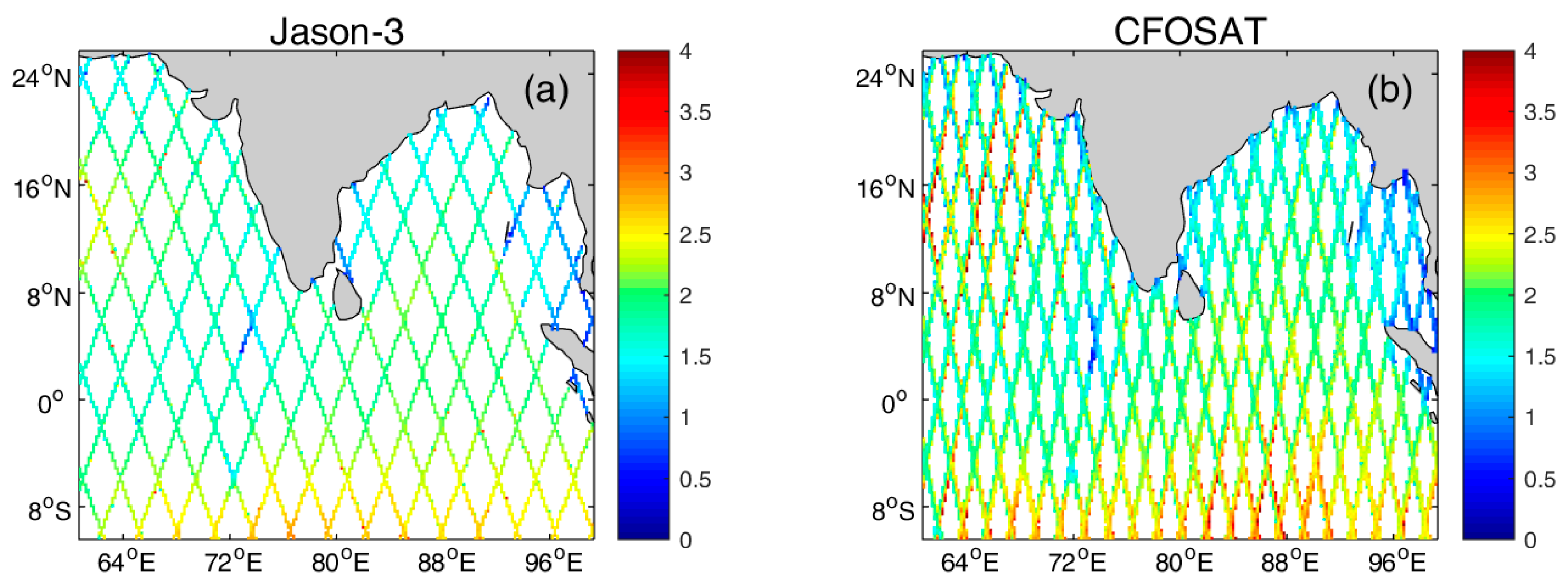
1]. By succeeding Topex/Poseidon, Jason-1, and Jason-2, Jason-3 extends the high-precision ocean altimetry data record, which was launched in January 2016. The China–France Oceanography Satellite (CFOSAT), which was launched in October 2018, carries the SWIM sensor [2]. SWIM provides a significant wave height at nadir-look and directional wave spectra with a wavelength cut-off of 70 m. This work aims to investigate the impact of the assimilation of SWH from Jason-3 in the MASNUM wave model on the Indian Ocean. Validation is performed with independent data from CFOSAT.
The purpose of wave data assimilation is to improve the wave model and to produce better performance. There are two main classes of assimilation methods: one is sequential methods, such as optimal interpolation (OI) [3] and ensemble Kalman filter (EnKF) [4], and the other is variational methods. Sequential methods implement independent corrections at different times, and variational methods aim to find the model solution that minimizes the differences between observations over the whole analysis period [5]. Sequential methods, which are relatively simple and require relatively low computing costs, confront the problem of specifying correlation scales in models and observations. At present, this issue is still one of the focuses in wave data assimilation.
There is no consolidated technique to spread altimeter data on a model grid. (1) Without spreading, only observations on the model grid replace model value [6,7]. (2) Exponential spreading function [8]. (3) Covariance of prediction error/background error/model error, which requires statistical determination and determines the information spread of observations. For the OI method, the prediction error correlation matrix, referred to as P, is assumed to be a function of correlation scale Lmax [5]. For the EnKF method, background-error covariance, referred as B, is constructed by ensemble members of model states. Apparently, B is flow-dependent, while P is not. It requires tremendous cost to run ensemble members of a wave model.
To reduce the computation cost, Sun et al. [9,
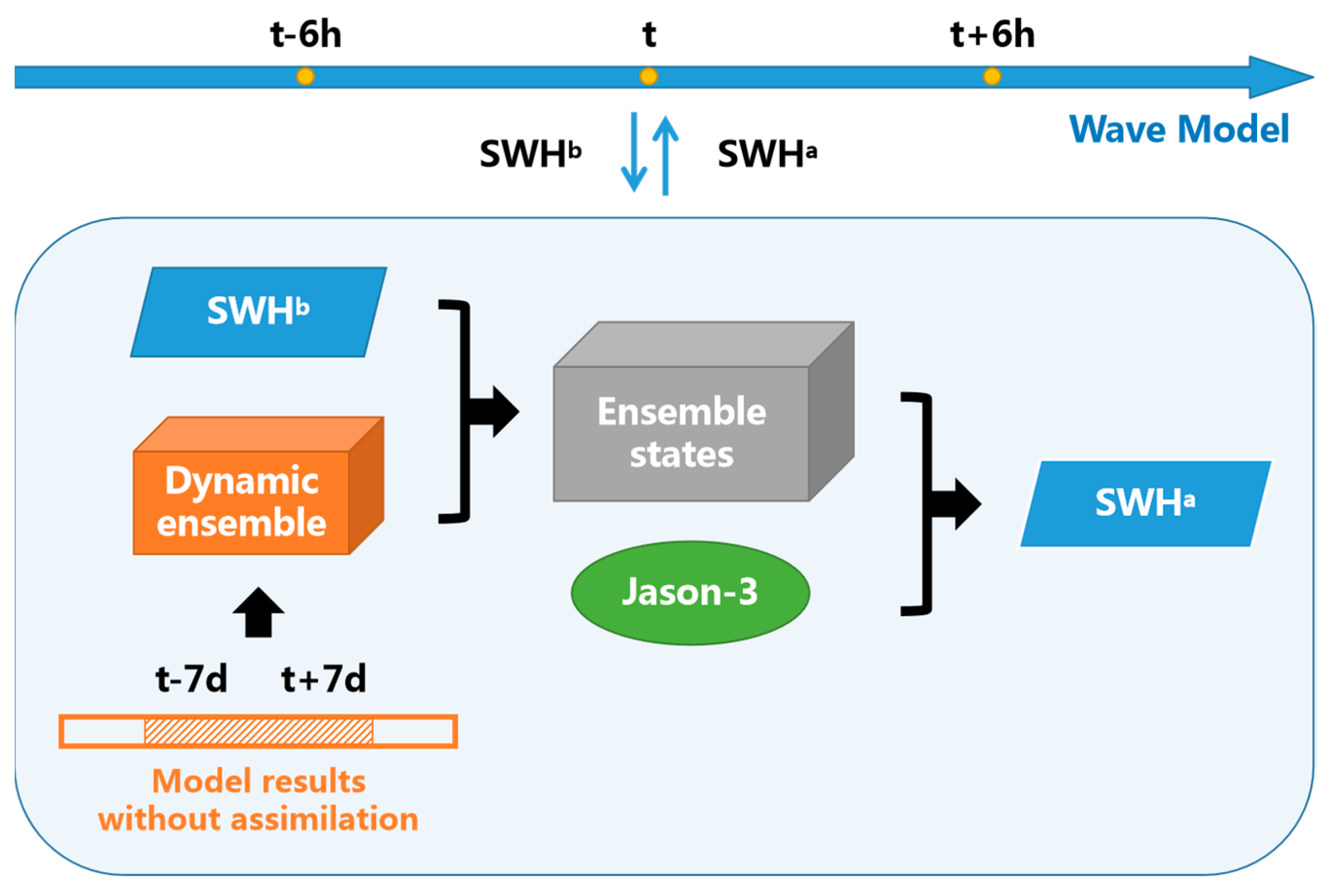
10], proposed the dynamic sampling method and static sampling method to construct background-error covariance by the differences between 24-h-interval significant wave heights. Therefore, construction of the model states requires only one model run instead of an ensemble of model runs. In this study, we will assimilate SWH of Jason-3 using a combination of ensemble adjust Kalman filter (EAKF) [11,12] and dynamic sampling method.
The paper is organized as follows. Section 2 briefly describes the wave model MASNUM, assimilation scheme, and satellite observations. Section 3.1 concerns the validation of the results with independent wave observations. The analysis of the assimilation impact in the case of high-sea state is presented in Section 3.2. Discussion and conclusions are given in Section 4 and Section 5, respectively.

2. Materials and Methods

2.1. Wave Model and Set-Up

The wave model used in this study is a third-generation global wave model Marine Sciences and Numerical Modeling (MASNUM) [13,14,15]. The complicated characteristic inlaid method is applied to integrate the wave energy spectrum balance equation. All governing equations have a physical meaning of the wave packet propagation along a ray. Thus, Yuan et al. [14] designed the characteristic inlaid computation scheme to reflect this property. A matching problem is solved between time and space steps using this scheme. In the model, the wave energy spectrum balance equation and its complicated characteristic equations are derived in a wave number space. The breaking dissipation source function adopts a theoretical result based on a statistical study of breaking waves [16].
MASNUM is implemented on a 15 × 15 km latitude–longitude grid that covers 60.7°E to 99.3°E and 10.4°S to 25.6°N; water depth of the domain is shown in Figure 1. The directional wave spectrum is discretized into 24 directions by a step of 15° and 25 frequencies ranging from 0.042 to 0.413 Hz. The propagation time step is 10 min. Output fields of integrated wave parameters are archived at 1-h intervals. The wave model MASNUM is driven by 1-h analyzed winds with 0.25 × 0.25° spatial resolution (ERA5) from the European Center for Medium-Range Weather Forecast (ECMWF) atmospheric model. The model topography is interpolated from a gridded bathymetric dataset (GEBCO) [17]. The wave spectrum of the open boundaries for the Indian Ocean domain are interpolated from the hourly output of an outer domain, which covers an area of 20°E to 145.5°E, 70°S to 45.5°N with a spatial resolution of 0.5 Deg.
Two runs of the wave model MASNUM were performed for the period from 1 July 2020 to 31 January 2021. The first run used the assimilation of Jason-3 altimeter wave heights (referred to as Run A). The second run is a baseline run of the wave model MASNUM without assimilation (referred to as Run B). For independent validation, we use observations of significant wave height from CFOSAT which are excluded from assimilation.

2.2. Assimilation Scheme

The assimilation procedure is split into two parts: first, the significant wave height of altimeter from the Jason-3 satellite is used to construct an analyzed field of SWH by assimilation technique using a combination of EAKF and dynamic sampling [10]. The second part consists of the reconstruction of the spectrum from the analyzed SWH. The information contained in the first-guess spectrum E b ( K , θ ) is used to produce an analyzed spectrum E a ( K , θ ) as E a ( K , θ ) = ( S W H a S W H b ) 2 E b ( K , θ ) [7]. Here, we use a limitation for the factor ( S W H a S W H b ) 2 to avoid introducing shocks in the model, i.e., if S W H a S W H b < 0.5 , we set the factor to the square of 0.5; if S W H a S W H b > 1.5 , we set the factor to the square of 1.5.
Flowchart of assimilation procedure is shown in Figure 2. In the process of assimilating, only one wave model member is implemented. The assimilation is performed sequentially every 6 h. SWH observations from Jason-3 are assimilated into the MASNUM wave model with the following scheme: (1) Dynamic ensemble, which is an approximation to background error, is constructed using the dynamic sampling method, i.e., collecting wave model results without assimilation on the interval (t − 7d, t + 7d) and then calculating the difference between 24 h-interval SWH fields. Here t represents assimilation time. Thus, dynamic ensemble changes with time. Specifically, dynamic ensemble is flow-dependent. There are 24 samples for each day. (2) The dynamic ensemble is superposed to the SWH field at time t to obtain ensemble states with 360 members. (3) The two-part filter method [11,12] is applied to update ensemble states using observations at time τ ( t 6 h , t + 6 h ) . (4) The analyzed SWH is the mean of the updated ensemble states. (5) An analyzed wave spectrum is reconstructed by multiplying the first-guess spectrum E b ( K , θ ) by the factor ( S W H a S W H b ) 2 .

2.3. Satellite Data

Jason-3 launched in January 2016 as the result of a joint effort by CNES, NASA, EUMETSAT, and NOAA. The satellite carries a typical suite of altimetry mission instruments that will acquire highly accurate measurements of ocean surface height to extend the data record compiled by Topex/Poseidon, Jason-1, and Jason-2 [18]. Jason-3 has an orbital repetition cycle of 10 days.
CFOSAT launched in October 2018 as a joint mission from the Chinese and French Space Agencies, devoted to the observation ocean surface wind and waves [19,20]. The mission contains two main instruments: a wave scatterometer called SWIM (surface wave investigation and monitoring), which provides significant wave height at nadir-look direction and directional wave spectra with a wavelength cut-off 70 m, and the wind scatterometer (SCAT). CFOSAT has an orbital repetition cycle of 13 days.
The data from Jason-3 and CFOSAT have been downloaded from the CMEMS web portal (Copernicus Marine Environment Monitoring Service, https://marine.copernicus.eu/ accessed on 17 July 2021). The domain is well covered by Jason-3 and CFOSAT. SWH from the satellites have been generated on a grid size that is 0.2 × 0.2°. There are 300,000 points collected from Jason-3, and 260,000 points collected from CFOSAT from 1 July 2020 to 31 January 2021. The spatial distribution of SWH based on the observations of Jason-3 and CFOSAT is shown in Figure 3. The distance between adjacent orbit tracks of CFOSAT is closer compared to that of Jason-3. There are two high-value regions of significant wave height in the domain, which are in the northwest and the south Indian Ocean.

3. Results

Two runs of the wave model MASNUM were performed for the period from 1 July 2020 to 31 January 2021. The first run used the assimilation of Jason-3 altimeter wave heights (referred to as Run A). The second run is a baseline run of the wave model MASNUM without assimilation (referred to as Run B).
First, we analyzed the impact, which consists of comparing model outputs from Runs A and B with independent wave observations of SWH from CFOSAT. This impact evaluates the efficiency of the assimilation system. The performance of these two runs is discussed by computing the statistical parameters for significant wave heights. Moreover, the impact was analyzed based on a comparison between model outputs with and without assimilation. This indicates how large the difference of wave parameters induced by the assimilation is. Another impact is considered and this consists of comparing model outputs with observations along orbit tracks from CFOSAT, especially in high-sea conditions.

3.1. Validation

In this section, we use the significant wave heights from CFOSAT as independent wave observations. SWH from the MASNUM wave model was first collocated with CFOSAT satellite data, which is along the orbit track using temporal–spatial interpolation. Statistical parameters on the difference between the observed and model wave variables were computed with the following definitions:
Mean   error   ( ME ) = M i O i ¯
Root   Mean   Square   Error   ( RMSE ) = ( M i O i ) 2 ¯
Mean   Absolute   Error   ( MAE ) = | M i O i | ¯
Relative   Error   ( RE ) = | M i O i | / O i ¯
Improvement   Rate   ( IR ) = Error noasm Eerror asm Error noasm %
Correlation   Coefficient ( Corr ) = M i   O i ¯   M ¯   O ¯ M i 2 ¯ M ¯ 2   O i 2 ¯ O ¯ 2
Scatter   index   ( SI ) = [ ( M i M ¯ ) ( O i O ¯ ) ] 2 ¯ O ¯
Table 1 shows the statistical parameters for Runs A and B. First, this indicates that the wave model MASNUM generally underestimates the significant wave height. After the assimilation of Jason-3 SWH data, the root mean square errors are reduced from 0.36 m to 0.32 m. Improvement rates of simulation error are more than 10%. This indicates that the MASNUM wave model reproduces relatively well the observed wave regimes, which are recorded by CFOSAT. The impact of assimilation is statistically weak given the applied high number of observations (number is roughly 260,000). Therefore, further detailed analysis is necessary.
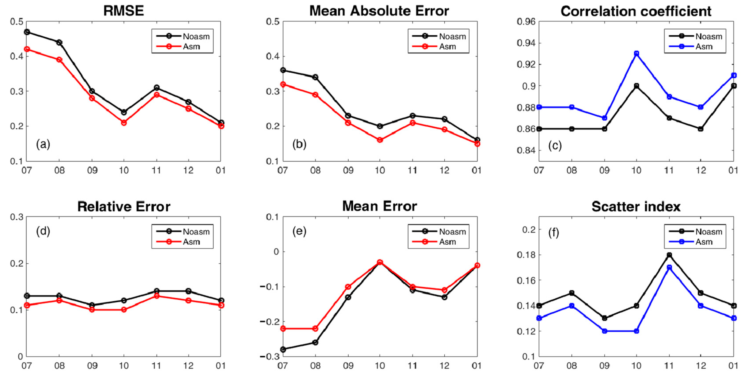
Statistical parameters for each month from 1 July 2020 to 31 January 2021 are shown in 
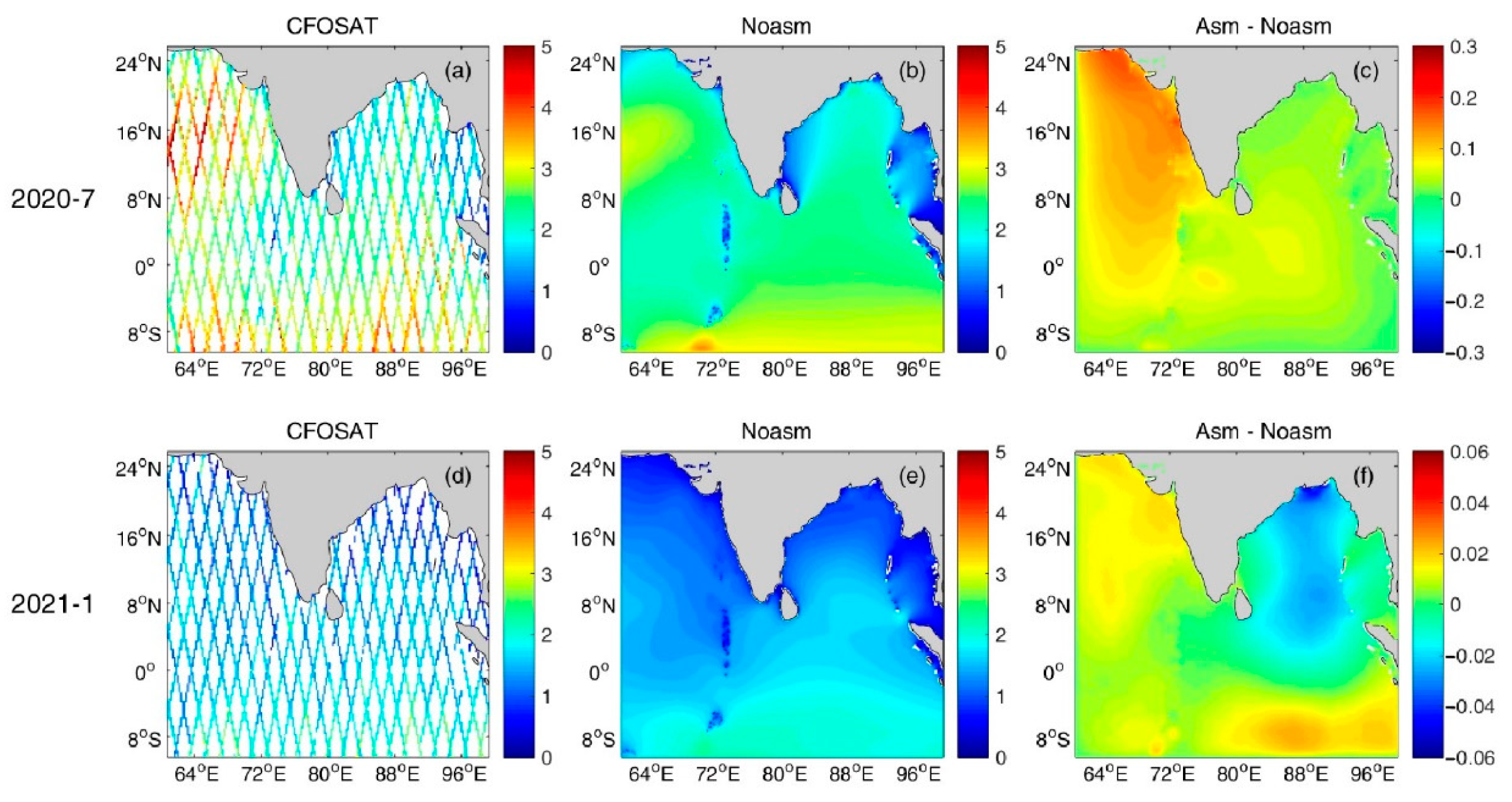
Figure 4. There is a similar tendency of RMSE and MAE, with maximum value in July and minimum value in January. However, there is little difference of relative error between each month. This is correlated with seasonal variation of surface waves in the Indian Ocean. As can be seen, SWH from CFOSAT in Figure 5a,d, monthly mean wave height in winter is less than 3 m, while in summer it is in the 2–5 m range. The comparison with CFOSAT indicates a correction of assimilation in July is more noticeable, i.e., the impact of assimilation is more remarkable in high-sea conditions. In Figure 4c, the correlation coefficient increased after data assimilation. Figure 4f indicates that scatter index decreased after data assimilation.
Comparisons between model outputs with and without assimilation indicate the difference of wave parameters induced by the assimilation. Figure 5c,f show the difference of SWH between Run A (with assimilation) and Run B (without assimilation) in July 2020 and January 2021, respectively. This clearly indicates that the monthly mean impact of the assimilation on significant wave height can reach roughly 0.2 m in July and ±0.03 m in January. SWH of CFOSAT and of wave model without assimilation in July are shown in Figure 5a,b. It is easy to see the strong impact of assimilation in the northwest Indian Ocean where the model is underestimating the significant wave height.

3.2. Analysis in High-Sea Conditions

The assimilation of Jason-3 altimeter wave data was analyzed for high-sea conditions in this section. Several cases are selected to evaluate the impact of assimilation. Generally, due to the propagation effect of ocean surface waves, wave data from Jason-3 are assimilated in one place. The impact of assimilation could be observed by CFOSAT at another place later. We attempt to detect this relationship using wave parameters and investigate the impact of assimilation.

3.2.1. Case A

Group velocity Cg, which describes the energy propagation of ocean surface waves, is given as follows.
ω = 2 π T ,   ω 2 = g k ,   λ = 2 π k ,   C = λ T ,   C g = 1 2 C
where ω and T represent frequency and period respectively, k and λ indicate wave number and wavelength separately, g represents gravitational acceleration. C is wave phase velocity.
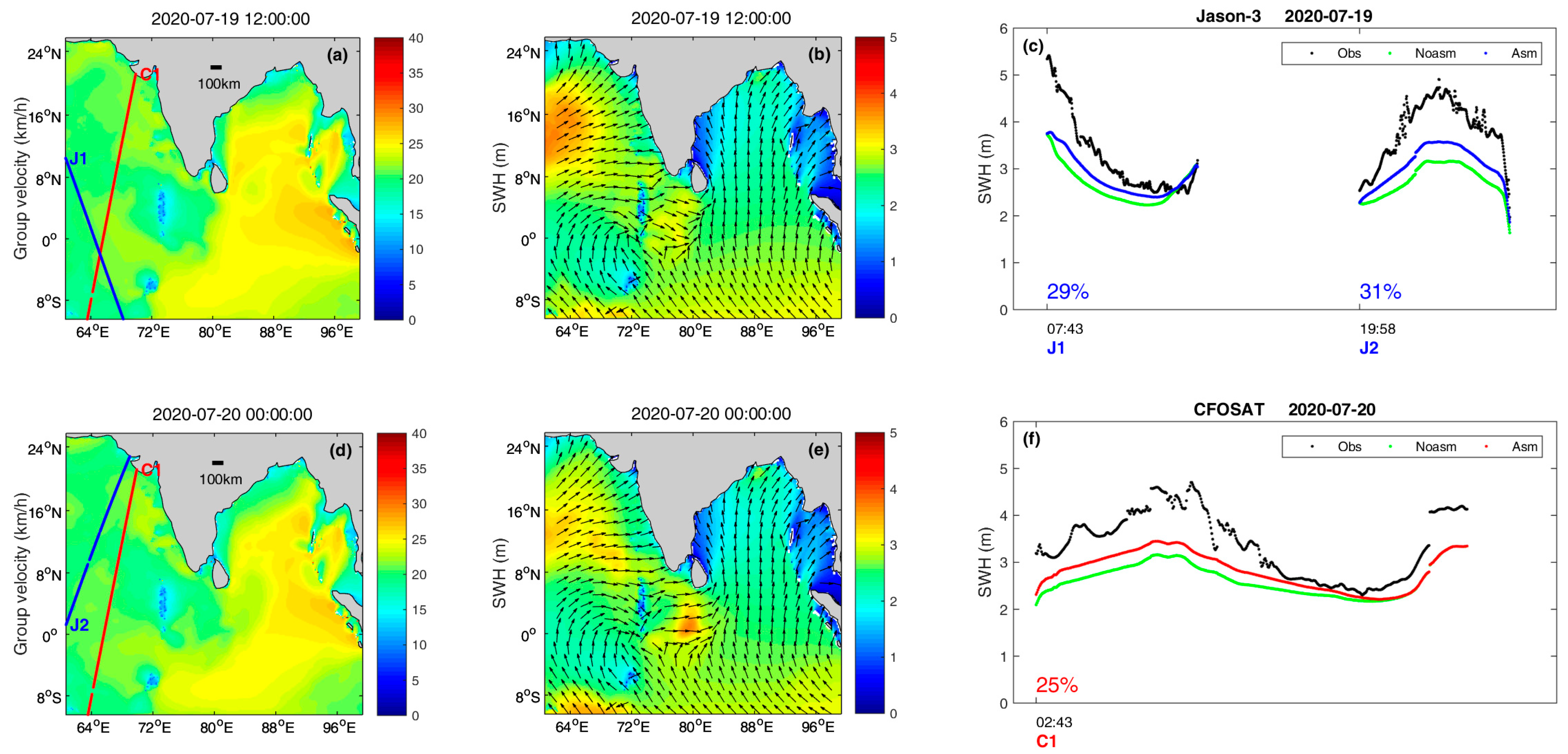
SWH time series at orbit tracks on 19–20 July 2020 are shown in Figure 6, referred to as Case A. In Figure 6c, black dot lines indicate observations of Jason-3, and blue lines and green lines represent SWH of the model with and without assimilation of Jason-3. Locations of orbit tracks J1 and J2 are shown in Figure 6a,d. Mean absolute error of SWH of model outputs decreased 29% and 31% at orbit tracks J1 and J2 compared to measurements of Jason-3.
We found that there is one orbit track of CFOSAT near orbit track J1 and J2, which is referred to as C1. The location of orbit track C1 is shown in Figure 6a,d. In Figure 6f, black dot lines represent the measurements of CFOSAT, and red lines and green lines indicate SWH of the wave model with and without assimilation of Jason-3. Improvement rate of mean absolute error of SWH is 25% at orbit track C1 compared with independent observations of CFOSAT.
Based on a mean wave period of the model without assimilation, group velocity Cg on 20 July 2020 at 0:00 UTC are shown in Figure 6d. SWH and mean wave direction are given in Figure 6e. Orbit track J2 and C1 differ by 6–7 h. At orbit track J2, group velocity is roughly 20 km/h and ocean surface waves propagated northeast. The first half of orbit track C1, where correction of assimilation is pronounced, is approximately 120–140 km from orbit track J2. This clearly indicates the efficiency of assimilation.
Group velocity Cg on 19 July 2020 at 12:00 UTC is shown in Figure 6a. SWH and mean wave direction are given in Figure 6b. Orbit track J1 and C1 differ by 19 h. Group velocity is roughly 20 km/h at orbit track J1. Ocean surface waves propagated northeast to the north of the crossing of J1 and C1, and propagated northwest at the south of the crossing simultaneously. Propagation distance is roughly 380 km, which covers orbit track C1. There is little influence of assimilation on the latter half of orbit track C1. One reason for that is the large time difference between the two orbits. The other reason is that the correction of assimilation in the latter half of orbit track J1 is relatively small.

3.2.2. Case B

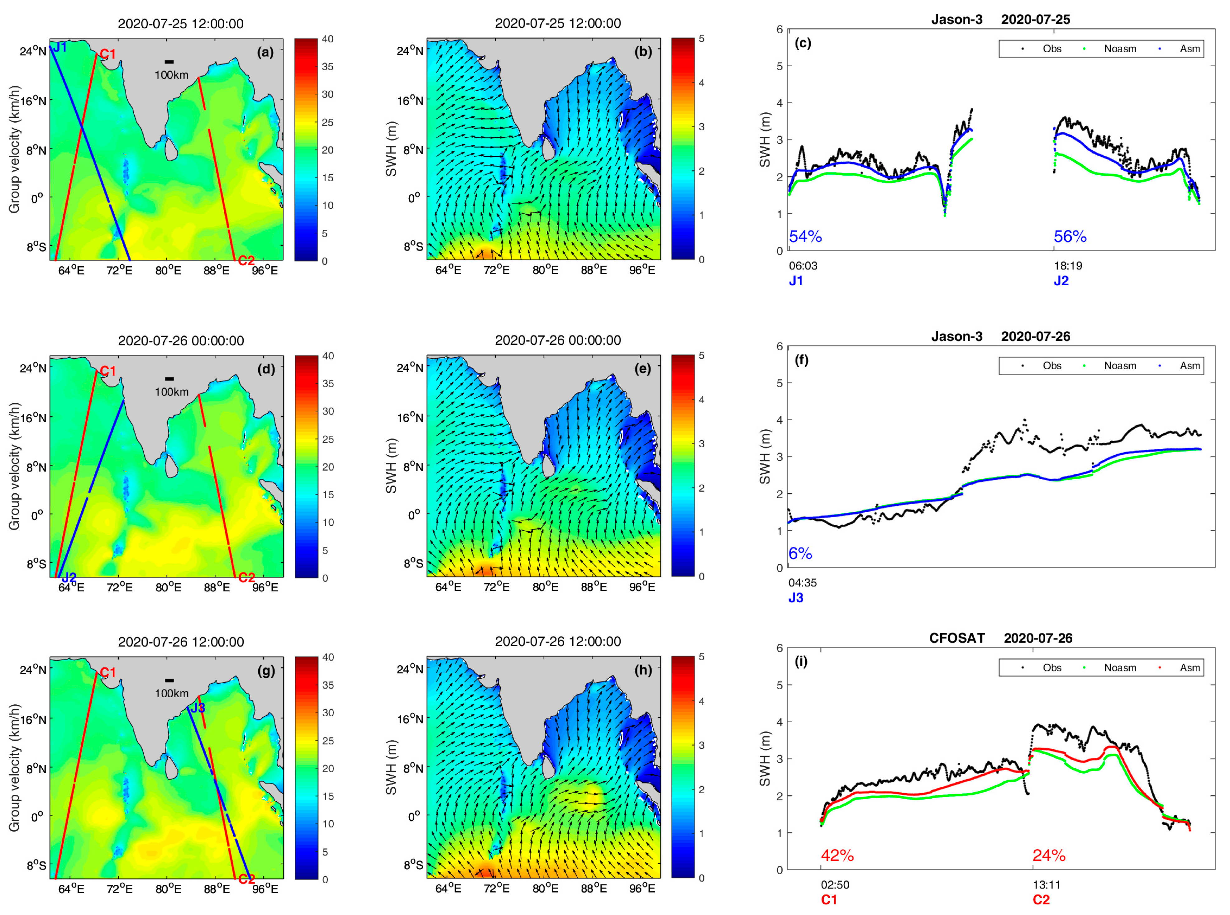
SWH time series at orbit tracks on 25–26 July 2020 are shown in Figure 7, referred to as Case B. In Figure 7c,f, black dotted lines indicate observations of Jason-3, and blue lines and green lines represent SWH of model with and without assimilation of Jason-3. Locations of orbit tracks J1/J2/J3 are shown in Figure 7a,d,g. Mean absolute error of SWH of the model outputs decreased 54%, 56%, and 6% at orbit tracks J1/J2/J3 compared to measurements of Jason-3.
We found that there are two orbit tracks of CFOSAT near orbit tracks J1/J2/J3, which are referred to as C1/C2. Locations of orbit tracks C1/C2 are shown in Figure 7a,d,g. In Figure 7i, black dotted lines represent measurements of CFOSAT, and red lines and green lines indicate SWH of the wave model with and without assimilation of Jason-3. Improvement rate of mean absolute error of SWH is 42% and 24% at orbit tracks C1/C2 compared with independent observations of CFOSAT.
Based on mean wave period of model without assimilation, group velocity Cg on 26 July 2020 at 12:00 UTC is shown in Figure 7g. SWH and mean wave direction are given in Figure 7h. Orbit track J3 and C2 differ by 9 h. In the latter half of orbit track J3, group velocity is roughly 23 km/h and ocean surface wave propagated towards northwest. Propagation distance is roughly 210 km, which covers orbit track C2, and the performance of assimilation is obvious at the first half of orbit track C2. Figure 7b,e,h show that significant wave height near 8°S increased gradually from 25 July 12:00 to 26 July 12:00. This indicates that ocean waves are potentially growing in the latter half of orbit track J3. Despite a small correction at orbit track J3, the impact of assimilation gradually amplifies with the propagation of surface waves.
Group velocity Cg on 26 July 2020 at 0:00 UTC is shown in Figure 7d. SWH and mean wave direction are given in Figure 7e. Orbit track J2 and C1 differ by 8 h. Surface waves in the latter half of orbit track J2 propagated northeast and away from the orbit track C1, therefore there is no influence of the former on the latter. At the first half of orbit track J2, group velocity is roughly 23 km/h and ocean surface wave propagated northwest. Propagation distance is roughly 190 km, which covers orbit track C1, and the performance of assimilation is remarkable at the latter half of orbit track C1.
Group velocity Cg on 25 July 2020 at 12:00 UTC is shown in Figure 7a. SWH and mean wave direction are given in Figure 7b. Orbit track J1 and C1 differ by 21 h. Surface wave at orbit track J1 propagated towards northeast mostly, thus there is little impact of assimilation on orbit track C1 at the south of the crossing of J1 and C1. At the north of the crossing, group velocity at the first half of orbit track J1 is roughly 20 km/h. Propagation distance of influence of assimilation is roughly 420 km, which covers orbit track C1. The impact of assimilation gradually weakens with long-range propagation of surface waves, therefore correction in the first half of the orbit track C1 is not pronounced.

3.2.3. Case C

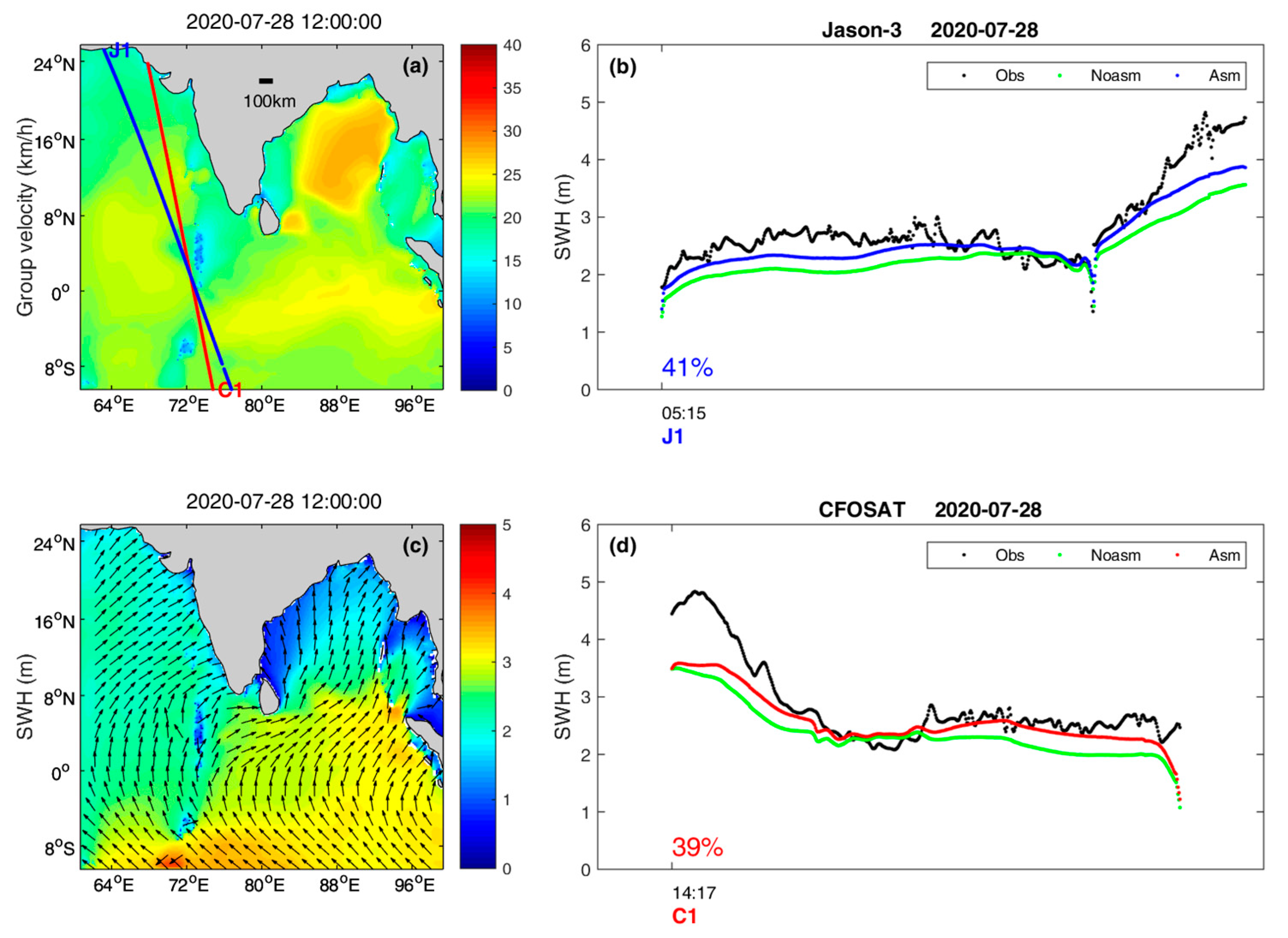
SWH time series at orbit tracks on 28 July 2020 are shown in Figure 8, referred to as Case C. In Figure 8b, black dotted lines indicate observations of Jason-3, and blue lines and green lines represent SWH of the model with and without assimilation of Jason-3. Location of orbit tracks J1 is shown in Figure 8a. Mean absolute error of SWH of the model outputs decreased 41% at orbit tracks J1 compared to measurements of Jason-3.
We found that there is one orbit track of CFOSAT near orbit track J1, which is referred to as C1. The location of orbit track C1 is shown in Figure 8a. In Figure 8d, black dotted lines represent measurements of CFOSAT, and red lines and green lines indicate SWH of the wave model with and without assimilation of Jason-3. Improvement rate of mean absolute error of SWH is 39% at orbit track C1 compared with independent observations of CFOSAT.
Based on mean wave period of model without assimilation, group velocity Cg on 28 July 2020 at 12:00 UTC is shown in Figure 8a. SWH and mean wave direction are given in Figure 8c. Orbit track J1 and C1 differ by 9 h. At the north of the crossing of J1 and C1, ocean surface waves propagated northeast at group velocity of roughly 23 km/h. At the south of the crossing, they propagated northwest at group velocity of roughly 25 km/h. SWH at the whole orbit track C1 are corrected by assimilation. This illustrates that mean wave direction is one of the indispensable elements in analysis of propagation of assimilation.

3.2.4. Case D

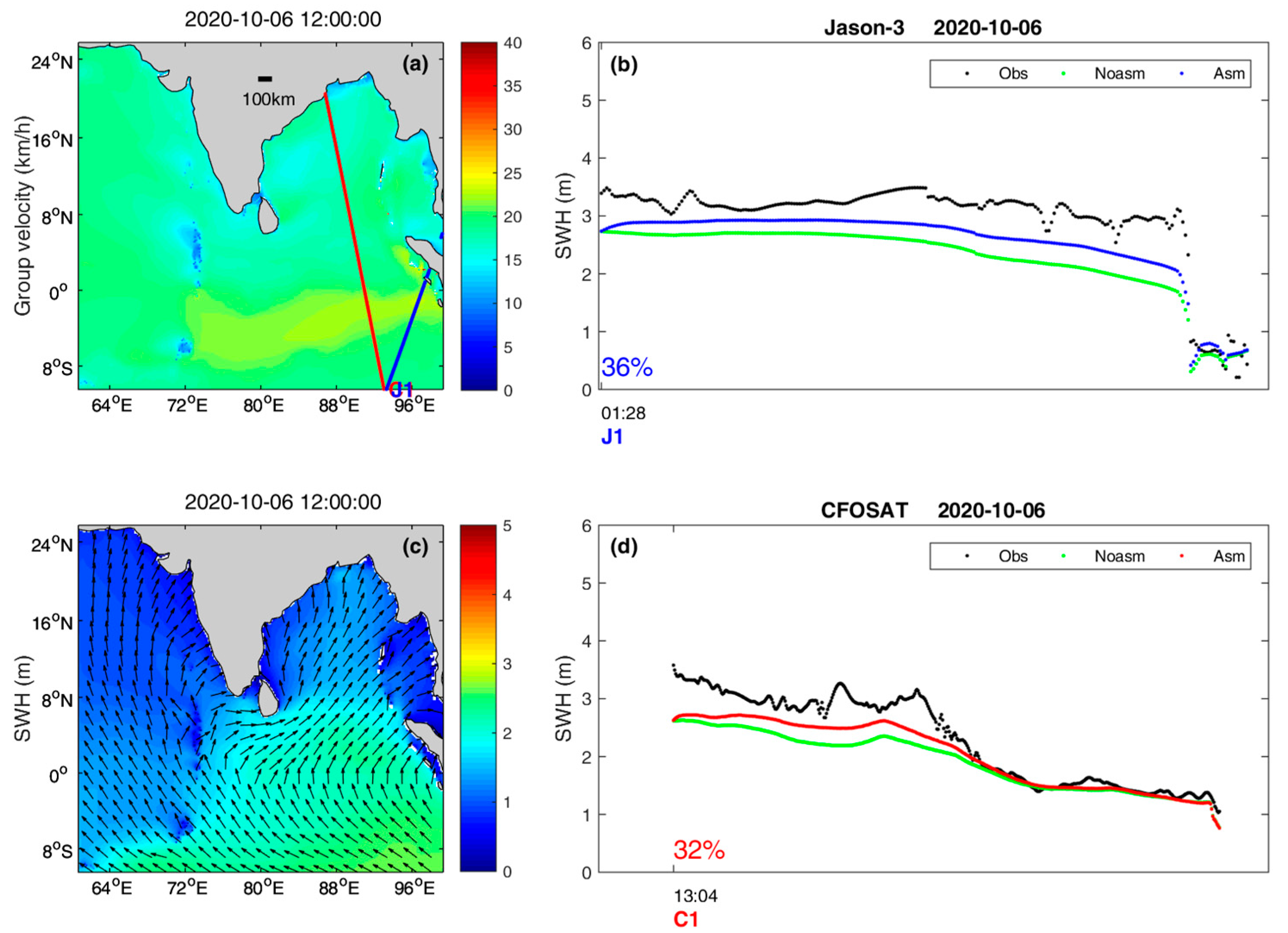
SWH time series at orbit tracks on 6 October 2020 are shown in Figure 9, referred to as Case D. In Figure 9b, black dotted lines indicate observations of Jason-3, blue lines and green lines represent SWH of model with and without assimilation of Jason-3. The location of orbit track J1 is shown in Figure 9a. Mean absolute error of SWH of model outputs decreased 36% at orbit track J1 compared to measurements of Jason-3.
We found that there is one orbit track of CFOSAT near orbit track J1, which is referred to as C1. The location of orbit track C1 is shown in Figure 9a. In Figure 9d, black dotted lines represent measurements of CFOSAT, and red lines and green lines indicate SWH of the wave model with and without assimilation of Jason-3. The improvement rate of mean absolute error of SWH is 32% at orbit track C1 compared with independent observations of CFOSAT.
Based on mean wave period of the model without assimilation, group velocity Cg on 6 October 2020 at 12:00 UTC is shown in Figure 9a. SWH and mean wave direction is given in Figure 9c. Orbit track J1 and C1 differ by 12 h. At orbit track J1, group velocity is roughly 20 km/h and ocean surface waves propagated northwest. The first half of orbit track C1, where correction of assimilation is considerable, is approximately 240 km from orbit track J1. This clearly indicates the efficiency of assimilation. This also illustrates that length of orbit track is one of decisive factors of the influence range of assimilation.

4. Discussion

The assimilation of observations from satellites is an efficient way to correct numerical model errors. In this study, measurements of SWH from Jason-3 are assimilated to improve MASNUM wave model outputs in the Indian Ocean. Validation is constructed by comparing significant wave height from model runs with and without assimilation against observations from CFOSAT. The period of assimilation experiments is from 1 July 2020 to 31 January 2021. Background errors are constructed by dynamic sampling instead of ensemble members of model runs. Variable state ensemble is updated using the EAKF method. During the assimilating procedure, only one member of a wave model is needed, which reduces the computation resource requirements.
Validation of model results indicates that mean absolute error of significant wave height reduces roughly 10% after assimilation. The monthly statistic of model error indicates that the wave model underestimates wave height in high-sea conditions. Significant wave height of model results with assimilation in July 2020 increased by roughly 0.1–0.3 m in the northeast of the Indian Ocean compared with that of the baseline run. In this study, several cases in high-sea conditions were analyzed. The improvement rate of mean absolute error reached roughly 20–40% at a single orbit track. Analysis confirms that observations along orbit tracks from Jason-3 are assimilated in one place, and the impact of assimilation propagates with ocean waves and then could be observed by CFOSAT in another place.
The wave scatterometer SWIM carried by CFOSAT provides a combined directional wave spectra from several incidence angles with an azimuthal cut-off of 70 m for wavelength. Based on the dynamic sampling method, preliminary experiments with assimilation of wave spectrum from CFOSAT will be developed in further study.

5. Conclusions

Based on observations of significant wave height from the satellites CFOSAT and Jason-3, the effect of wave data assimilation in the MASNUM wave model for the Indian Ocean was analyzed and evaluated. Ensemble states of SWH were constructed by dynamic sampling method rather than by an ensemble of wave model members. This approach reduces the computational cost dramatically. Comparison between model outputs and measurements along orbit tracks indicated that assimilation improves model results remarkably in high-sea conditions. This study also analyzed several factors that affected independent validation of assimilation.

Author Contributions

Conceptualization, M.S. and Y.Y.; methodology, M.S., X.Y.; software, M.S., J.D.; validation, M.S., J.D.; formal analysis, M.S., Y.Y.; investigation, M.S.; resources, Y.Y.; data curation, M.S., J.D.; writing—original draft preparation, M.S.; writing—review and editing, Y.Y., J.D.; visualization, M.S.; supervision, Y.Y., X.Y.; project administration, Y.Y.; funding acquisition, M.S., Y.Y., and J.D. All authors have read and agreed to the published version of the manuscript.

Funding

This research was jointly funded by the National Key Research Program of China, grant number 2017YFC1404201, Basic Scientific Fund for National Public Research Institutes of China, grant number 2019Q07 and 2019Q06, and National Natural Science Foundation of China, grant number 41906186 and 41906028, Qingdao Postdoctoral Science Foundation QDBSH2019005.

Acknowledgments

We acknowledge the data support from the European Center for Medium-Range Weather Forecast (ECMWF, http://www.ecmwf.int/, accessed on 17 July 2021), the Copernicus Marine Environment Monitoring Service (CMEMS, https://marine.copernicus.eu/, accessed on 17 July 2021), AVISO (https://www.aviso.altimetry.fr/en/home.html, accessed on 17 July 2021), GEBCO (https://www.gebco.net/, accessed on 17 July 2021). We thank the reviewers for their careful reading and valuable comments, which helped us to improve the manuscript.

Conflicts of Interest

The authors declare no conflict of interest.

References

  1. Law-Chune, S.; Aouf, L.; Dalphinet, A.; Levier, B.; Drillet, Y.; Drevillon, M. WAVERYS: A CMEMS global wave reanalysis during the altimetry period. Ocean Dyn. 2021, 71, 357–378. [Google Scholar] [CrossRef]
  2. Hasselmann, K.; Chapron, B.; Aouf, L.; Ardhuin, F.; Collard, F.; Engen, G.; Schulz-Stellenfleth, J. The ERS SAR wave mode: A breakthrough in global ocean wave observations. Eur. Space Agency ESASP 2012, 1326, 167–197. [Google Scholar]
  3. Hollingsworth, A. Objective analysis for numerical weather prediction. J.M.S.J. 1986, 64, 11–59. [Google Scholar] [CrossRef] [Green Version]
  4. Evensen, G. Sequential data assimilation with a nonlinear quasi-geostrophic model using Monte Carlo methods to forecast error statistics. J. Geophys. Res. Space Phys. 1994, 99, 10143–10162. [Google Scholar] [CrossRef]
  5. Lionello, P.; Günther, H.; Janssen, P.A.E.M. Assimilation of altimeter data in a global third-generation wave model. J. Geophys. Res. Space Phys. 1992, 97, 14453–14474. [Google Scholar] [CrossRef]
  6. Janssen, P.A.E.M.; Lionello, P.; Reistad, M.; Hollingsworth, A. Hindcasts and data assimilation studies with the WAM model during the Seasat period. J. Geophys. Res. Space Phys. 1989, 94, 973–993. [Google Scholar] [CrossRef]
  7. Esteva, D.C. Evaluation of preliminary experiments assimilating Seasat significant wave heights into a spectral wave model. J. Geophys. Res. Space Phys. 1988, 93, 14099. [Google Scholar] [CrossRef]
  8. Francis, P.E.; Stratton, R.A. Some experiments to investigate the assimilation of SEASAT altimeter wave height data into a global wave model. Q. J. R. Meteorol. Soc. 1990, 116, 1225–1251. [Google Scholar] [CrossRef]
  9. Sun, M.; Yin, X.; Yang, Y. Construction and application in global wave data assimilation of static sample set. Oceanologia Lim-nologia Sinica 2014, 45, 918–927. [Google Scholar] [CrossRef]
  10. Sun, M.; Yin, X.; Yang, Y.; Wu, K. An effective method based on dynamic sampling for data assimilation in a global wave model. Ocean Dyn. 2017, 67, 433–449. [Google Scholar] [CrossRef]
  11. Anderson, J.L. An ensemble adjustment Kalman filter for data assimilation. Mon. Weather Rev. 2001, 129, 2884–2903. [Google Scholar] [CrossRef] [Green Version]
  12. Anderson, J.L. A local least squares framework for ensemble filtering. Mon. Weather Rev. 2003, 131, 634–642. [Google Scholar] [CrossRef] [Green Version]
  13. Yuan, Y.; Pan, Z.; Hua, F.; Sun, L. LAGFD-WAM wave numerical model (I), the basic physical model. Acta Oceanol. Sin. 1992, 14, 1–7. [Google Scholar]
  14. Yuan, Y.; Hua, F.; Pan, Z.; Sun, L. LAGFD-WAM numerical wave model-II. Characteristics inlaid scheme and its application. Acta Oceanol. Sin. 1992, 14, 12–24. [Google Scholar]
  15. Yang, Y.; Qiao, F.; Zhao, W.; Teng, Y.; Yuan, Y. MASNUM ocean wave numerical model in spherical coordinates and its application. Acta Oceanol. Sin. 2005, 27, 1–7. [Google Scholar] [CrossRef]
  16. Yuan, Y.; Tung, C.C.; Huang, N.E. Statistical Characteristics of Breaking Waves. In Wave Dynamics and Radio Probing of the Ocean Surface; Phillips, O.M., Hasselmann, K., Eds.; Springer: Boston, MA, USA, 1986; pp. 265–272. [Google Scholar] [CrossRef]
  17. GEBCO. Available online: https://www.gebco.net/ (accessed on 17 July 2021).
  18. AVISO. Available online: https://www.aviso.altimetry.fr/en/home.html (accessed on 17 July 2021).
  19. Hauser, D.; Tison, C.; Amiot, T.; Delaye, L.; Mouche, A.; Guitton, G.; Aouf, L.; Castillan, P. CFOSAT: A new Chinese-French satellite for joint observations of ocean wind vector and directional spectra of ocean waves. Remote Sens. Oceans Inland Waters Tech. Appl. Chall. 2016, 9878, 98780. [Google Scholar] [CrossRef] [Green Version]
  20. Hauser, D.; Tison, C.; Amiot, T.; Delaye, L.; Corcoral, N.; Castillan, P. SWIM: The First Spaceborne Wave Scatterometer. IEEE Trans. Geosci. Remote Sens. 2017, 55, 3000–3014. [Google Scholar] [CrossRef] [Green Version]
Figure 1. Study domain with water depth. Unit is meters.
Remotesensing 13 03833 g001
Figure 2. Flowchart of wave assimilation.
Remotesensing 13 03833 g002
Figure 3. Significant wave height of satellite Jason-3 and CFOSAT from 1 July 2020 to 31 January 2021. Unit is meters. (a) SWH from satellite Jason-3; (b) SWH from satellite CFOSAT.
Remotesensing 13 03833 g003
Figure 4. Statistics of model results against observations from CFOSAT satellite computed every month during the period from 1 July 2020 to 31 January 2021. (a) Root mean square error; (b) Mean absolute error; (c) Correlation coefficient; (d) Relative error; (e) Mean error; (f) Scatter index.
Remotesensing 13 03833 g004
Figure 5. Spatial distribution of SWH (in meters) in July 2020 and January 2021. (a) SWH of CFOSAT in July 2020; (b) SWH of MASNUM wave model without assimilation in July 2020; (c) Difference of SWH with and without assimilation of Jason-3 wave data in July 2020; (d) SWH of CFOSAT in January 2021; (e) SWH of MASNUM wave model without assimilation in January 2021; (f) Difference of SWH with and without assimilation of Jason-3 wave data in January 2021.
Remotesensing 13 03833 g005
Figure 6. Case A: SWH time series at orbit tracks on 19–20 July 2020. (a,d): Color represents group velocity in km/h. Blue and red dotted lines indicate orbit tracks of Jason-3 and CFOSAT, respectively. Location of character J1/J2/C1 indicates the start of the orbit track. (b,e): Color and arrows represent SWH and mean wave direction of model outputs without assimilation. (c) Black dotted lines indicate Jason-3 measurements; blue and green lines indicate SWH of model outputs with and without assimilation of Jason-3; percentage represents improvement rate of mean absolute error of SWH with assimilation compared to without assimilation. (f) Black dotted lines indicate CFOSAT measurements; red lines and green lines indicate SWH of model outputs with and without assimilation of Jason-3; percentage represents improvement rate of mean absolute error of SWH with assimilation compared to without assimilation.
Remotesensing 13 03833 g006
Figure 7. Case B: SWH time series at orbit tracks on 25–26 July 2020. (a,d,g): Color represents group velocity in km/h. Blue and red dotted lines indicate orbit tracks of Jason-3 and CFOSAT, respectively. Location of character J1/J2/J3/C1/C2 indicates the start of the orbit track. (b,e,h): Color and arrows represent SWH and mean wave direction of model outputs without assimilation. (c,f): Black dotted lines indicate Jason-3 measurements; blue and green lines indicate SWH of model outputs with and without assimilation of Jason-3; percentage represents improvement rate of mean absolute error of SWH with assimilation compared to without assimilation. (i) Black dotted lines indicate CFOSAT measurements; red lines and green lines indicate SWH of model outputs with and without assimilation of Jason-3; percentage represents improvement rate of mean absolute error of SWH with assimilation compared to without assimilation.
Remotesensing 13 03833 g007
Figure 8. Case C: SWH time series at orbit tracks on 28 July 2020. (a) Color represents group velocity in km/h. Blue and red dotted lines indicate orbit tracks of Jason-3 and CFOSAT, respectively. Location of character J1/C1 indicates the start of the orbit track. (b) Black dotted lines indicate Jason-3 measurements; blue and green lines indicate SWH of model outputs with and without assimilation of Jason-3; percentage represents improvement rate of mean absolute error of SWH with assimilation compared to without assimilation. (c) Color and arrows represent SWH and mean wave direction of model outputs without assimilation. (d) Black dotted lines indicate CFOSAT measurements; red lines and green lines indicate SWH of model outputs with and without assimilation of Jason-3; percentage represents improvement rate of mean absolute error of SWH with assimilation compared to without assimilation.
Remotesensing 13 03833 g008
Figure 9. Case D: SWH time series at orbit tracks on 6 October 2020. (a) Color represents group velocity in km/h. Blue and red dotted lines indicate orbit tracks of Jason-3 and CFOSAT, respectively. Location of character J1/C1 indicates the start of the orbit track. (b) Black dotted lines indicate Jason-3 measurements; blue and green lines indicate SWH of model outputs with and without assimilation of Jason-3; percentage represents improvement rate of mean absolute error of SWH with assimilation compared to without assimilation. (c) Color and arrows represent SWH and mean wave direction of model outputs without assimilation. (d) Black dotted lines indicate CFOSAT measurements; red lines and green lines indicate SWH of model outputs with and without assimilation of Jason-3; percentage represents improvement rate of mean absolute error of SWH with assimilation compared to without assimilation.
Remotesensing 13 03833 g009
Table 1. Statistical analysis of significant wave heights from runs with and without assimilation at orbit tracks of CFOSAT. The period of analysis is from 1 July 2020 to 31 January 2021.
ErrorRun B: NoasmRun A: AsmImprovement Rate
Mean error−0.15−0.1313%
RMSE0.360.3211%
Mean absolute error0.260.2312%
Relative error0.130.1115%
Correlation coefficient0.910.92--
Scatter index0.160.15--
Publisher’s Note: MDPI stays neutral with regard to jurisdictional claims in published maps and institutional affiliations.

