Efficient Transformer for Remote Sensing Image Segmentation

Abstract

Semantic segmentation for remote sensing images (RSIs) is widely applied in geological surveys, urban resources management, and disaster monitoring. Recent solutions on remote sensing segmentation tasks are generally addressed by CNN-based models and transformer-based models. In particular, transformer-based architecture generally struggles with two main problems: a high computation load and inaccurate edge classification. Therefore, to overcome these problems, we propose a novel transformer model to realize lightweight edge classification. First, based on a Swin transformer backbone, a pure Efficient transformer with mlphead is proposed to accelerate the inference speed. Moreover, explicit and implicit edge enhancement methods are proposed to cope with object edge problems. The experimental results evaluated on the Potsdam and Vaihingen datasets present that the proposed approach significantly improved the final accuracy, achieving a trade-off between computational complexity (Flops) and accuracy (Efficient-L obtaining 3.23% mIoU improvement on Vaihingen and 2.46% mIoU improvement on Potsdam compared with HRCNet_W48). As a result, it is believed that the proposed Efficient transformer will have an advantage in dealing with remote sensing image segmentation problems.

1. Introduction

Remote sensing (RS) is capable of collecting information from objects with no physical contact through satellite and aerial-based platforms and is widely applied in geological survey, urban resources management, and disaster monitoring [1,2]. To achieve a high performance in the aforementioned applications, an automatic and fast detection method for ground objects with high accuracy in a robust way is desirable. The deep learning method, a pioneering method in remote sensing area that develops rapidly, with high accuracy, robustness, and fast inference speed, is widely used in object detection and classification tasks.

Semantic segmentation, as a method of deep learning, is used to classify pictures at the pixel level. Therefore, this method can describe the information contained in a picture to the greatest extent, including the category, position, and image proportion of each object [3]. Currently, there are two kinds of models to solve image segmentation problems, one is the convolution neural network (CNN)-based model and the other is the transformer architecture based model. It is acknowledged that, with the increase of training data in the remote sensing area, a CNN-based model will reach a threshold; however, on the contrary, a transformer-based model can continuously improve the performance [4]. To this end, to segment remote sensing images with massive data, the transformer-based model can realize its full potential.

The remote sensing image segmentation performance is highly related to two factors: the acquisition of spatial information and the establishment of global relations [5]. Spatial information is also called structural information, referring to the texture, shape and structured information of the image. In CNN structure, spatial information is inevitably damaged because it relies on convolution and pooling operations to extract features and reduce the image resolution [6].

However, the transformer structure utilizes a serialization process for the image and introduces position embedding to describe the position relationship instead of requiring convolution and pooling operations, and thus the spatial information of the original image can be kept [7]. Global relation describes the semantic relationship between categories, which can be efficiently established by using attention mechanism.

An attention mechanism is the main component of a transformer structure, which aims to obtain the feature representations through bridging the relationship between each pixel; therefore, global relations are established from beginning to end. However, the vanilla CNN structure does not have an attention mechanism, and, even if the attention mechanism is introduced in CNN, the performance is far weaker than the transformer structure. To this end, the transformer structure outperforms the CNN structure regarding to the acquisition of spatial information and the establishment of global relations. Therefore, the transformer architectures are widely applied in segmentation tasks to replace CNNs.

Vision transformer [8] is the first transformer architecture in computer vision, outperforming the CNN-based methods in a large margin at image-level classification task. However, it is not adequate for the segmentation task since the decoder (also called segmentation head) is not introduced here. SETR [9] based on the vision transformer architecture introduces segmentation components and, finally, achieved state-of-the-art performance on the segmentation task.

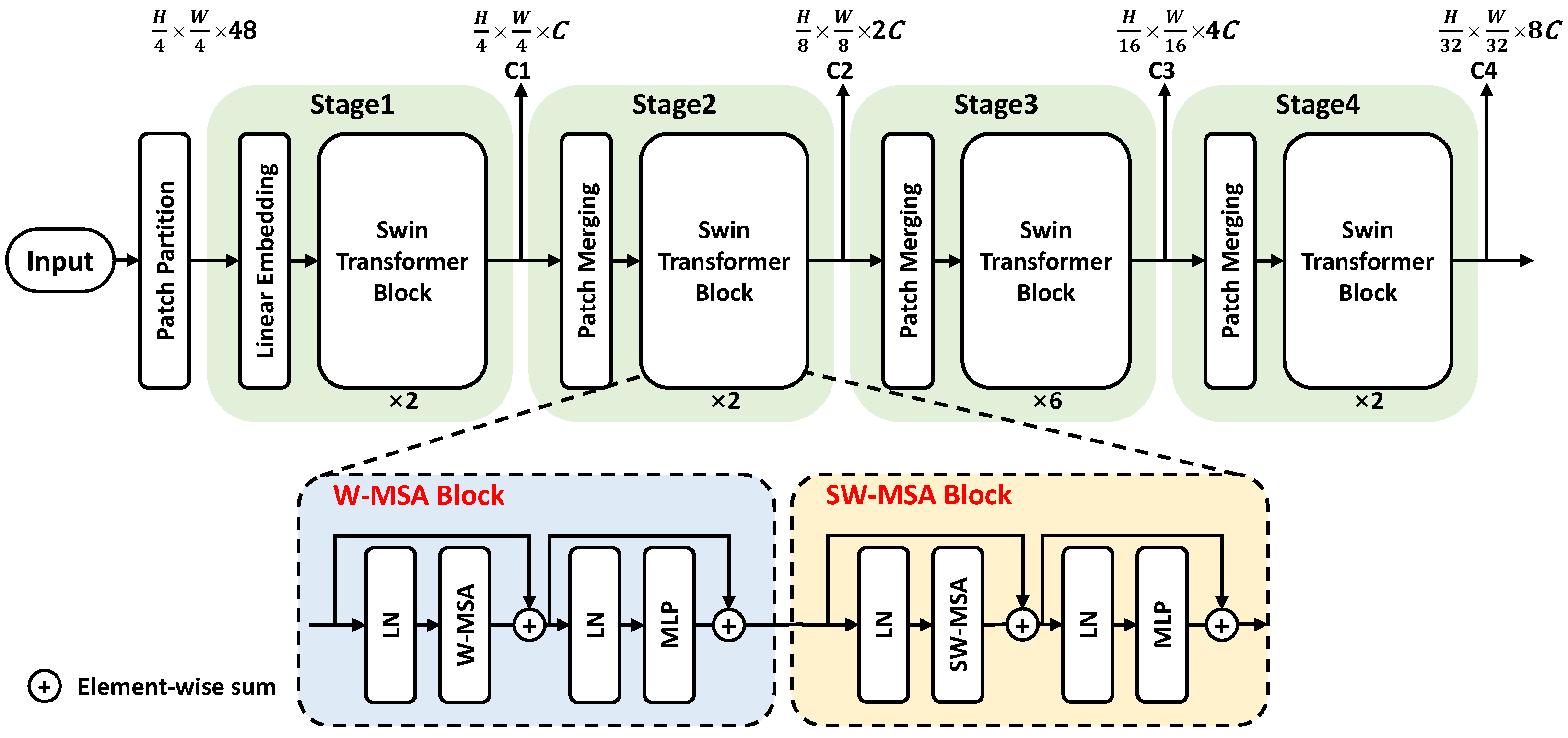
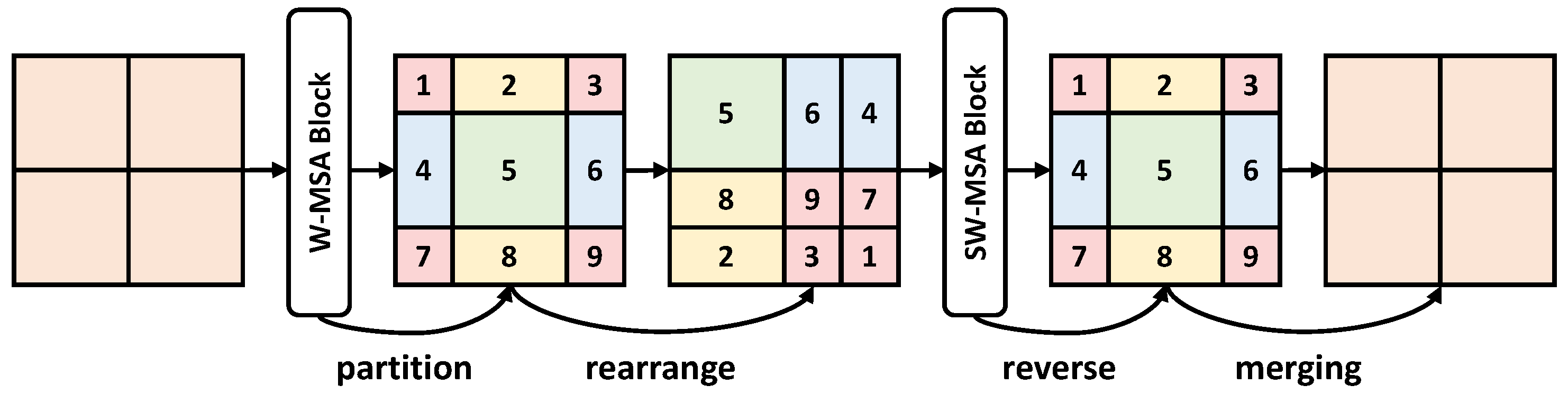
Although SETR explores a feasible way of applying the transformer in the segmentation task, it is inefficient to obtain spatial information and with a high computation load. To cope with the aforementioned drawbacks, we introduce the shifted window transformer (Swin transformer [10]), which adopts a hierarchical transformer block to obtain multi-scale features, which is useful to obtain spatial information.

Although the Swin transformer has achieved better performance on segmentation tasks compared with basic transformer, there are two main problems to be addressed for the remote sensing image segmentation task. First, high efficiency is required since the massive data collected by satellite platforms will cost plenty of computing resources. Second, blurry edge and irregular edge caused by the relative movement of the objects and satellite platforms heavily impairs the segmentation performance.

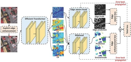
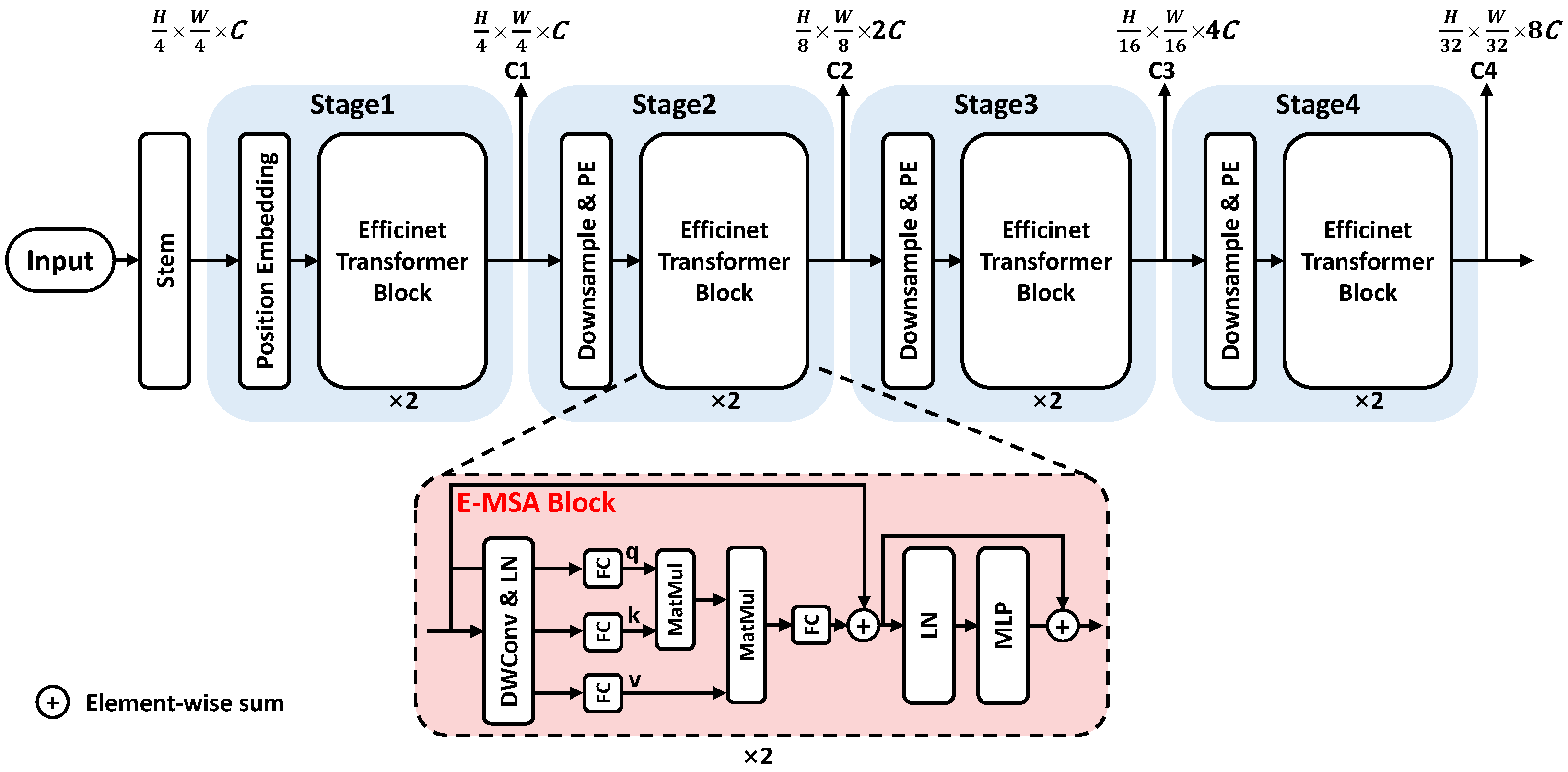
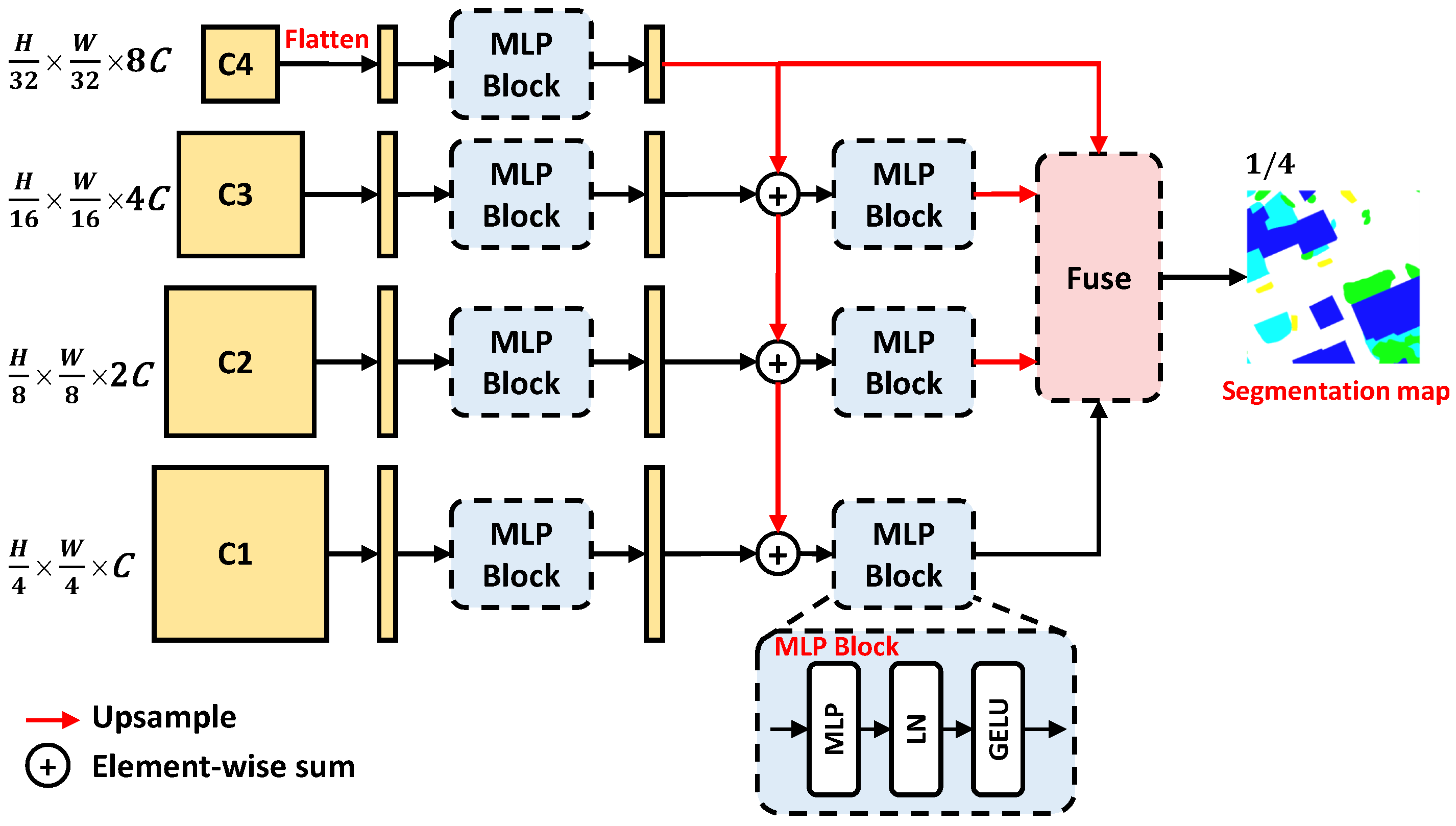
In this paper, we propose the following well-designed architecture to make the Swin transformer lightweight while improving the edge segmentation performance. First, we introduced an Efficient transformer backbone [11] to replace the original Swin transformer backbone at the first attempt by reducing the number of transformer blocks and applying a more lightweight transformer design to save the computation load. Second, we designed a pure transformer-based segmentation head called a multilayer perceptron head (mlphead) to replace the complex uperhead of the Swin transformer to further decrease the computational load and realize a pure transformer structure [12].

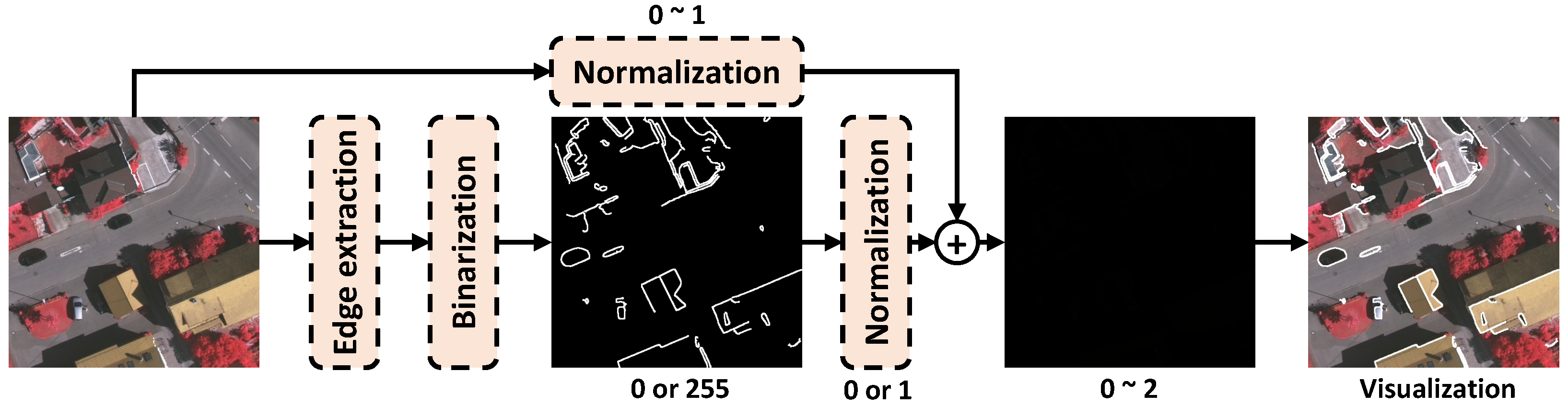
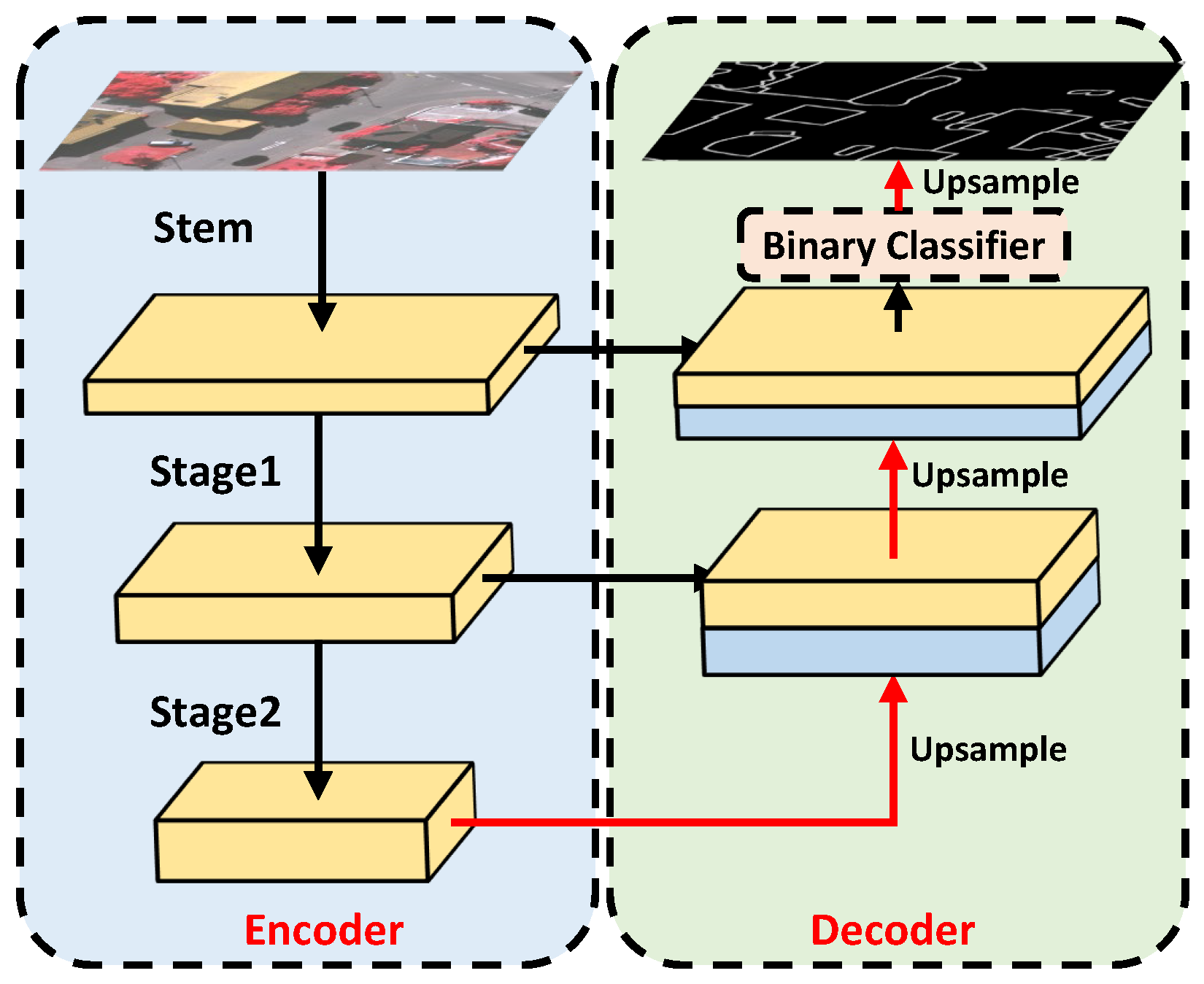
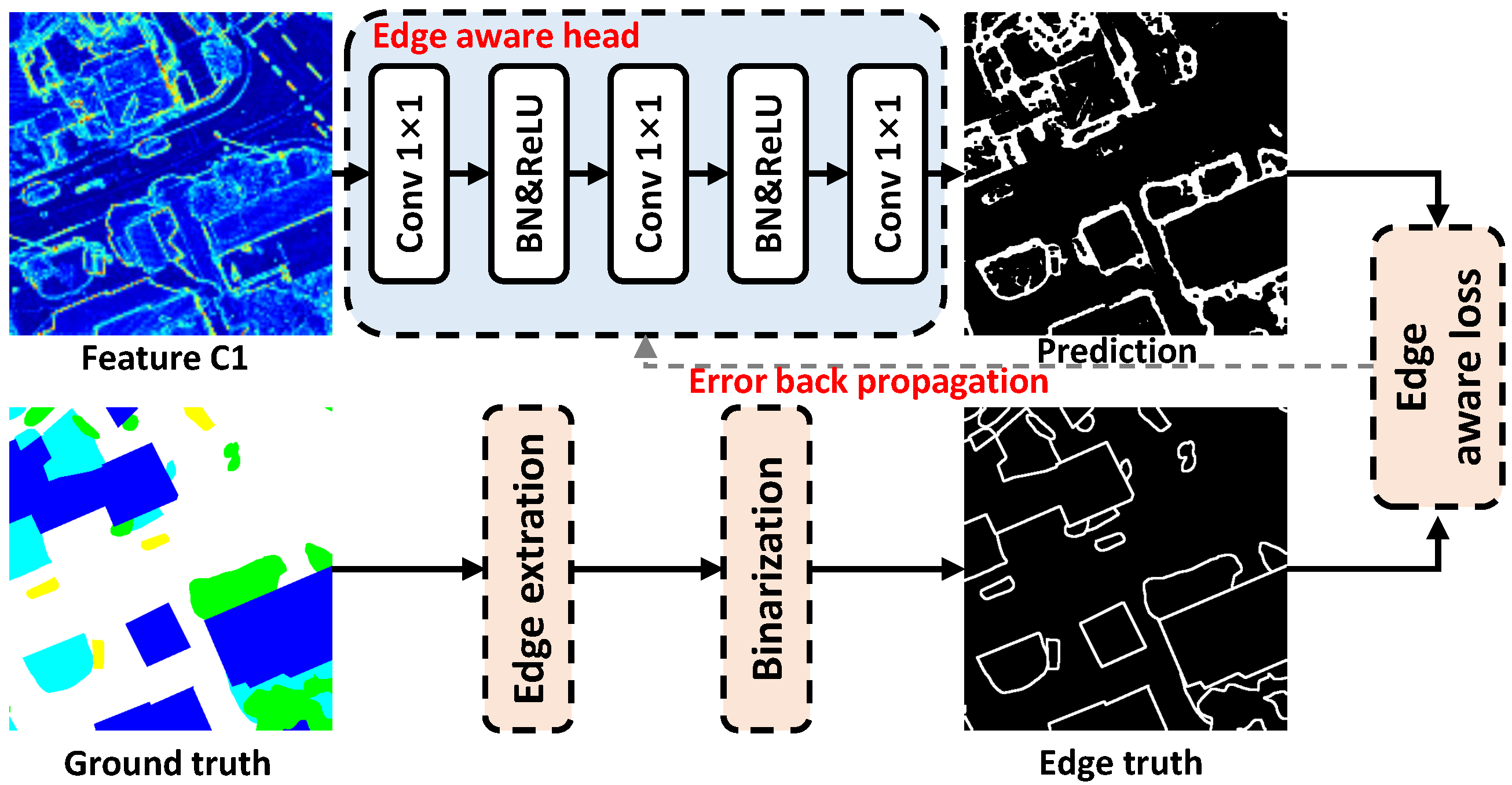
In particular, a pure transformer architecture can be helpful to accelerate the inference speed [13]. Then, in order to improve the edge segmentation performance, the hierarchical transformer designs are introduced in the Efficient transformer to generate multi-scale features that contain high-resolution features and high-level semantic features to rebuild edge details. Finally, the explicit edge enhancement and implicit edge enhancement methods are proposed to force the model to pay more attention to the segmentation of object edge.

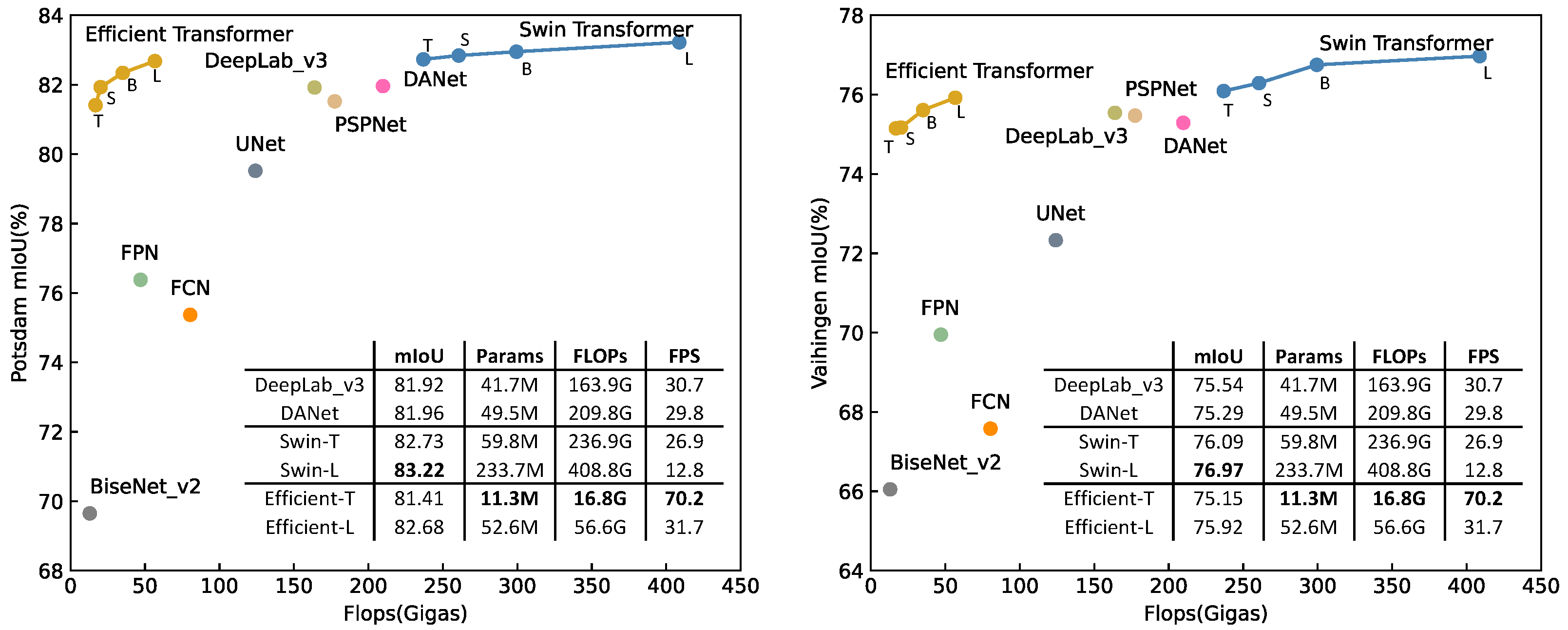
Two experimental datasets, Potsdam and Vaihingen, were adopted to evaluate the proposed methods, as can be seen in Figure 1, the proposed Efficient transformer achieved a trade off between computational complexity (Flops) and accuracy (mean intersection over union abbreviated as mIoU), and the Swin transformer surpassed CNN-based methods. The code is available at https://github.com/zyxu1996/Efficient-Transformer, accessed on 1 August 2021.

The main contributions of this work are summarized as follows:

• A Swin transformer was introduced to better establish the global relations and proved effective to achieve state-of-the-art performance on the remote-sensing Potsdam and Vaihingen datasets at the first attempt.
• A lightweight Efficient transformer backbone and pure transformer mlphead were proposed to reduce the computation load of Swin transformer and accelerate the inference speed.
• Explicit edge enhancement and implicit edge enhancement methods proposed to cope with the object edge extraction problem in the transformer architecture.

2. Related Work

In this section, some related work regarding state-of-the-art (SOTA) remote sensing applications and the model designs are introduced, including CNN-based models and transformer-based models, which provide experiences to resolve four main problems in remote sensing segmentation: the acquisition of spatial information, the reconstruction of edge details, the establishment of global relations, and lightweight architecture designs.

CNN-based models: CNN-based methods are specialized in obtaining local representations, hence the spatial information (e.g., shape and texture) and edge details are more concerned, yet the global relations are limited to local representations. The classical CNN architecture FCN [6] uses pooling layers to obtain features, which impairs the spatial information. First, to repair the spatial information decreased in the pooling operation, UNet [14] proposed a skip connection to bridge shallow layers and deep layers, thus, finding the lost spatial information from shallow layers.

Second, to obtain the sharp edge, BARNet [15] proposed a boundary-aware (also called edge-aware) loss embedded on a multi-level feature fusion block to obtain a sharp semantic edge. HRCNet [5] combined boundary-aware loss and boundary-aware module to improve the edge segmentation results on tiny objects. Third, as for the establishment of global relations, multi-scale fusion and attention mechanisms were introduced in CNN architectures. 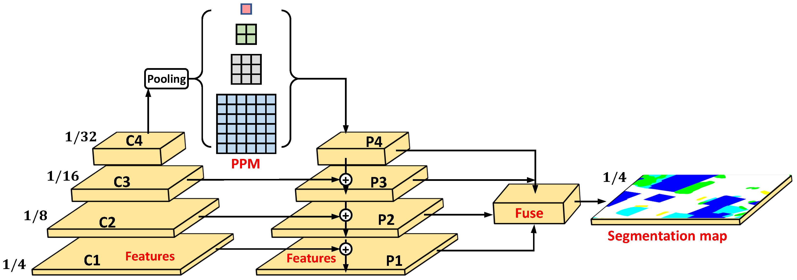DeepLab [16] proposed atrous spatial pyramid pooling (ASPP) to obtain different receptive field information so that the model could establish the relation between local and global. PSPNet [17] proposed the pyramid pooling module (PPM) to directly fuse information from different scales, leading to fused information from different regions.

The FPN [18] structure designed a cascade addition operation to fuse multi-scale features step by step, thus, making the final segmentation results suited for multi-scale inputs. DANet [19] employs the self-attention mechanism to build the relation between local pixel and global pixels by calculating the coefficient matrix of the local pixel to obtain the contributions of global pixels and leading to good performance on the Cityscapes dataset. Finally, a lightweight design is required after adding many extra modules.

GCNet [20] adopted a simplified self-attention mechanism to establish global relations and achieves a similar performance but costs less computation resources. Instead of building the relations between pixels, SENet [21] designed a learnable module to obtain the weights of each channel to establish the relations in the channel dimension and greatly reduced the computation load. BiseNet [22,23] and MobileNet [24,25] used well-designed lightweight backbones to realize real-time inferring in mobile devices.

Among all the aforementioned CNN models, the problems of spatial information extraction, edge reconstruction, and lightweight designs are solved to some extent; however, the global relations establishment is far from resolved.

Transformer-based models: Transformer architecture is good at establishing global relations since the attention-mechanism-based designs compose the basic transformer unit but are less robust at extracting local information. Therefore, by referring to CNN designs, the transformer architecture can perfectly resolve the four problems. A shift from CNNs to transformers recently began with the Vision transformer (ViT [8]), which is the first work to apply the transformer structure to image tasks.

Based on the pioneering work, many following works made improvements. First, to obtain the spatial information, SETR [9] and TransUNet [26] adopted the skip connections (proposed by UNet [14]) to connect shallow layers and deep layers, which first surpassed CNN-based models in segmentation tasks. However, the ViT variants, such as SETR and TransUNet, have high computation complexity, damaging the application of the transformer in segmentation tasks.

Therefore, a lightweight transformer design is urgently needed. Second, to make the transformer architecture lightweight, SegFormer [27] proposed a simple and efficient design without positional encoding and uses a simple decoder (segmentation head) to obtain the final segmentation results, thus, achieving a competitive performance to the models with the same complexity. ResT [11] designed an efficient transformer block to reduce the computation load of the original transformer backbone. Third, although these transformers established global relations and also applied lightweight designs, the edge processing is rarely mentioned.

Moreover, uncertain edge definitions are common in the ground truth of remote sensing images, which affected the performance [28]. To deal with such edge problems, three approaches are introduced here: (a) Fusing high-resolution features is helpful to restore the edge information as these features usually retain more complete structure and edge details [29]. (b) Using smoother upsampling methods can ensure a smoother edge of the object [18]. (c) Edge enhancement approaches, such as edge supervision [5], are capable of urging the model to pay more attention to the object edge, learning more detailed edge information.

Finally, to resolve the four problems, we first adopt the transformer-based architecture where the global relations establishment have been perfectly realized. Then, we use the hierarchical transformer design to obtain spatial information. We propose the Efficient transformer model, which contains an efficient transformer backbone and pure transformer mlphead to achieve lightweight designs. Finally, the explicit and implicit edge enhancement methods are proposed to deal with the blurry edge problem.

3. Methods

A Swin transformer backbone with the uperhead model has proved its effectiveness and excellent performance on semantic segmentation datasets but not on remote sensing segmentation datasets [10]. This paper makes a thorough study of applying a Swin transformer on remote sensing segmentation and proposes an Efficient transformer backbone, pure transformer segmentation head named mlphead, explicit edge enhancement and implicit edge enhancement methods to cope with three main shortcomings of Swin transformer: high computation load, low inference speed, and low ability to extract edge details. The details of each component are introduced as follows.

3.1. Investigation of Basic Swin Transformer Backbone and Uperhead

Semantic segmentation models are usually composed of the backbone and segmentation head. Backbone is used to extract the features from the image so that the model can distinguish different pixel categories. The segmentation head maps the features extracted from the backbone to specific classification categories and restores the downsampled features to the resolution of the input image.

3.1.1. Swin Transformer Backbone

The structure of the Swin transformer backbone is shown in Figure 2. The overall framework is composed of a Patch Partition module and four cascade stages to produce four resolution outputs. The stage1 contains Linear Embedding and two Swin Transformer Blocks, the remaining stages contain a Patch Merging module and an even number (e.g., ×2) of blocks in each stage. Every two blocks are composed of a window multi-head self-attention (W-MSA) block and a shifted windows multi-head self-attention (SW-MSA) block to calculate the global attention.

A detailed W-MSA Block contains layer normalization (LN), a W-MSA module, and a multilayer perceptron (MLP). LN normalizes the features to make the training process more stable, W-MSA is used to calculate the attention relation between pixels, and MLP contains a large number of learnable parameters to record the learned coefficients of W-MSA. The concrete process is shown as follows, given a $H\times W\times 3$ input (3 represents the RGB channel). The Patch Partition module first partitions the image into several $\frac{H}{4}\times \frac{W}{4}\times 3$ windows and flattens it into sequence with a length of $4\times 4\times 3=48$.

Therefore, the original resolution of $H\times W$ becomes $\frac{H}{4}\times \frac{W}{4}$, and the dimension is changed from 3 to 48. Then, the Linear embedding maps the feature dimensions from 48 to C and feeds the feature to Swin Transformer Blocks to establish the global relations. The Patch Merging adjusts the feature resolution before each stage to generate features with suitable resolutions.

Figure 2 displays the Swin transformer tiny version with 2, 2, 6, and 2 blocks in each stage. By adjusting the number of blocks in each stage and changing the value of dimensions C, this paper provides four versions of Swin transformers, namely tiny, small, base, and large, abbreviated as Swin-T, Swin-S, Swin-B, and Swin-L, meaning that the scale of the model changes from tiny to large.

The specific design of the Swin transformer is the W-MSA, compared to traditional MSA calculating the relation in the whole $H\times W$ image size, W-MSA calculates the attention relation in the $7\times 7$ window size, greatly reducing the amount of calculation. However, such a process also reduces the receptive field (e.g., from $H\times W$ to $7\times 7$), which is unfavorable for the segmentation of large objects. Therefore, the Swin transformer adopts an ingenious design called SW-MSA to tackle this problem (shown in Figure 3).

By partitioning and merging the feature map between two transformer blocks and extending the local receptive field to the global receptive field, the Swin transformer consists of four stages and performs $2\times$ spatial downsampling in the Patch Merging layer of each stage, where four outputs C1, C2, C3, and C4 denote different resolutions: $\frac{H}{4}\times \frac{W}{4}$, $\frac{H}{8}\times \frac{W}{8}$, $\frac{H}{16}\times \frac{W}{16}$, and $\frac{H}{32}\times \frac{W}{32}$, respectively. These outputs have different receptive fields from small to large; therefore, they are respectively sensitive to different sizes of objects.

3.1.2. Uperhead Introduction

Uperhead was first proposed with UperNet [30], presenting that the features with different resolutions were sensitive to different characters. For example, the $\frac{1}{4}$ resolution features make it easier to obtain texture information, and the $\frac{1}{32}$ resolution features are important for understanding the category of the scene. For semantic segmentation tasks, the texture and category of the object are equally paramount, and thus the outputs of different stages need to be fused to obtain a better segmentation performance.

As is depicted in Figure 4, the whole process includes a pyramid pooling module (PPM), cascade addition architecture, and fusion block. PPM uses global pooling with different pooling scales (1, 2, 3, and 6) to obtain information on different receptive fields so that the model establishes the relationship between local and global, thereby, enhancing the model’s ability to discriminate between different categories. After PPM, C4 becomes feature map P4.

The cascade addition architecture uses a step-by-step addition operation to fuse the outputs of different stages. Specifically, it upsamples P4 ($\frac{1}{32}$) and adds it to the input C3 ($\frac{1}{16}$) to obtain the fused features P3 ($\frac{1}{16}$) and then obtains P2($\frac{1}{8}$) and P1($\frac{1}{4}$) via the same operation. The fusion block fuses P1, P2, P3, and P4 to generate the fused features with $\frac{1}{4}$ resolution and applies a convolution layer to map the dimensions to the category numbers for the purpose to obtain the final segmentation map.

3.2. Efficient Architecture Design

As expressed in [31], the high computational complexity and energy requirements of deep learning methods typically limit their application in remote sensing platforms, such as on-board scenarios. Haut et al. [31] proposed utilizing a low-power hardware device to perform model inferring, which reduced the resource consumption. In another way, the efficient architecture designs of deep learning methods are also extremely important to save computing resources, which could further promote the application of deep learning methods in remote sensing scenarios.

3.2.1. Efficient Transformer Backbone

One of the challenging problems of applying the transformer structure in computer vision is the high computation load. The computational complexity of an attention block can be expressed as $\omega =4hw{C}^2+2{\left(hw\right)}^{2}C$, where C represents the dimensions, generally ranging from dozens to hundreds. Therefore, the computational complexity of the transformer is mainly determined by the input image size, whose computation complexity is quadratic to the image size. For a 2D input image, the computation load is very large. Thus, Swin transformer divides an $h\times w$ size image into $M\times M$ patches, and the final computational complexity becomes $\omega =4hw{C}^2+2M^{2}hwC$, changing the quadratic complexity into linear complexity [10].

The Efficient transformer block (E-MSA block) proposed in this paper establishes the local and global attention relationship by mapping $h\times w$ to a smaller $h^{{}^{\prime }}\times w^{{}^{\prime }}$, thereby, reducing the amount of calculation. When $h^{{}^{\prime }}\times w^{{}^{\prime }}$ is small enough, the Efficient transformer block will be more efficient than the Swin transformer, but the performance will also be damaged; therefore, we set h${}^{\prime }$ and w${}^{\prime }$ to $\frac{H}{32}$ and $\frac{W}{32}$ for a trade-off between the performance and efficiency.

In addition, when the task is relatively easy, to avoid the overfitting problem and reduce computational resource consumption, the number of blocks and dimensions of C can be reduced so that the model can reduce the complexity of the model almost without losing accuracy [11].

The detailed model structure is shown in Figure 5. Compared with the Swin transformer structure, there are three differences. First, the Efficient transformer uses convolution with a stride of 2 in each stage for patch embedding (PE) and downsampling the feature map. Second, before each transformer block, a depth-wise convolution (DWConv) is used to perform position embedding to learn the position information of each pixel, replacing the relative position embedding in the original Swin transformer.

Third, a lighter Efficient transformer block with $h^{{}^{\prime }}\times w^{{}^{\prime }}$ input size is used, applying fully connected layer (FC) to reduce dimensions and matrix multiplication (MatMul) to calculate attention relation, LN and MLP adopt traditional transformer designs. By applying the former structures, the Efficient transformer can achieve comparable accuracy to the Swin transformer but with less computation complexity.

3.2.2. Mlphead Design

A pure transformer structure is beneficial to perform inference accelerating, consisting of layer normalization (LN), multilayer perceptron (MLP), and multi-head self-attention block (MSA). In order to design a pure transformer segmentation head, the MLP is applied to extract features to replace the convolution layer. MSA is good at modeling global relations, but with limited contributions for segmentation head design since the backbone achieves this function well. Therefore, we combine MLP, LN, and GELU activation functions to form the MLP Block displayed in Figure 6.

In addition, we adopt the cascade addition architecture to fuse different scale features and to improve the segmentation of multi-scale objects. Especially, the MLP Block is designed to accept sequence input, and so we flatten the input 2D features before feeding them to the MLP Block. Finally, we obtain four branches’ outputs to be fed into the Fuse block, upsampled to the same $\frac{1}{4}$ resolution. By fusing the four resolution features to generate the output segmentation map, the final results can be well suited for different scale inputs.

3.3. Edge Processing

Edges are difficult to identify in semantic segmentation tasks. First, it is difficult to label the edge pixels accurately. Second, during the remote sensing image acquisition process, the camera and the ground objects are in relative motion, resulting in the distortion problem of the objects [32,33]. To cope with these two problems, two strategies are proposed, including explicit edge enhancement and implicit edge enhancement methods. Figure 7 displays the blurry edge in the images and inconsistent edge labeling in the ground truth.

3.3.1. Explicit Edge Enhancement

An explicit edge enhancement method called auxiliary edge fusion (AEF) is proposed in Figure 8. The image is added with the edge extracted by an edge extractor (e.g., canny edge extraction algorithm [34] or CNN-based edge extractor) to enhance the edge part. The specific process is shown below, first, using the edge extractor to obtain the segmentation edge of the object, and then mark the edge part and non-edge part to 255 and 0, respectively.

Then, the normalization block normalizes the value 255 of the pixel to 1. The above branch normalizes the image with the pixel value of 0∼255 to 0∼1. The edge and normalized image are added together to obtain an enhanced edge image with the pixel value of 0∼2. The enhanced edge image is visualized as the last picture visualization. As can be seen, the edge part is highlighted with white lines, which can enhance the model’s ability to discriminate the edge part.

Such an idea is based on our assumption that when the input image has accurate edge information, the pixel-level classification task can be transformed into a region-level classification task, thereby, greatly reducing the difficulty of image segmentation. Based on this hypothesis, we conduct the following verification. We first extract the edges according to the ground truth, and then apply the above-mentioned operations to obtain the enhanced image.

The results are shown in

Table 1. The results of extracting the edge from the ground truth.

Backbone	Edge	Recall (%)	Precision (%)	F1 (%)	OA (%)	mIoU (%)
Swin-B [10]	w/o	86.50	86.77	86.63	88.01	76.75
	w	98.15	97.28	97.71	98.08	95.55

, when the ground truth is used to generate the edge, we can consider that the generated edge is 100% correct. After using such a high-precision edge as supplementary information, the mIoU increased by an astonishing 18.8%. Therefore, if there are other high-precision methods instead of using the ground truth to generate an accurate edge, the supplement of this edge information will also bring a huge improvement.

To verify this, we first attempt to apply a simple canny edge extractor to obtain the edge, although the threshold of canny has been carefully selected, the extracted edge is far from the edge truth. Therefore, we design a CNN-based edge extractor to obtain a fine edge, which is closer to the edge truth. The CNN-based extractor is displayed in Figure 9; it is combined with an encoder-decoder architecture where ResNet [35] is the encoder to obtain edge representations, and UNet [6] is the decoder to restore edge details.

The final features are fed to a binary classifier to obtain edge and non-edge predictions. In particular, the edge extraction network is pre-trained and fixed before training the Efficient transformer. In the encoder part, every stem or stage operates $2\times$ downsampling to obtain feature representations; therefore, the features in the last stage are a $\frac{1}{8}$ resolution of the input. As high resolution features are beneficial to obtain edge details, a $\frac{1}{8}$ input resolution is a balance of edge information and semantic information. Through the CNN-based edge extractor, the prediction in the edge obtains further improvement.

3.3.2. Implicit Edge Enhancement

Implicit edge enhancement is mainly divided into two parts, namely edge supervision (ES) and edge enhancement loss (EEL). EEL is improved based on the commonly used segmentation loss namely cross-entropy loss. Edge supervision is implemented jointly by edge aware head and edge aware loss (see Figure 10). First, taking C1 as the input of the edge aware head, since C1 contains rich structural information, can achieve a good edge extraction effect.

The edge aware head is composed of a simple combination of 1 × 1 convolution layer (Conv 1×1), batch normalization (BN) and ReLU activation function to map the features to two categories including edge and non-edge part. After the edge aware head, edge prediction is generated. Then, the below ground truth goes through a simple edge extractor (a kind of morphological processing method [36]) to obtain the edge truth.

After that, the error of edge prediction and edge truth is calculated by the edge aware loss and is back-propagated to optimize the edge aware head. Through the implicit edge enhancement method, the model can focus on optimizing the edge in the training processing. The detailed definitions of edge enhancement loss and edge aware loss are shown in the following equations.

Edge aware loss (i.e., $Los{s}_{ea}$) is a binary classification loss, including edge and non-edge categories. As is shown in Equations (1) and (2), $p\left(x_i\right)$ denotes the probability of $x_i$ pixel classified as edge pixel, $1-p\left(x_i\right)$ means the probability of $x_i$ pixel not belonging to edge, and $\mathit{H}\left(x_i\right)$ represents the cross-entropy loss at this point $x_i$. $nu{m}_P$ and $nu{m}_N$ represent the number of edges and non-edge pixels, respectively, where $nu{m}_N$ is usually much larger than $nu{m}_P$. As a result, the points in the edge part can obtain a larger loss weight coefficient, meaning that the model will pay more attention to the learning of the edge part.

$$\mathit{H}\left(x_i\right)=-\mathit{p}\left(x_i\right)log\left(\mathit{p}\left(x_i\right)\right)-(1-\mathit{p}\left(x_i\right))log(1-\mathit{p}\left(x_i\right))$$

(1)

$${\mathit{Loss}}_{ea}=\frac{nu{m}_N}{nu{m}_P+nu{m}_N}\sum _{i=1}^{nu{m}_P}\mathit{H}\left(x_i\right)+\frac{nu{m}_p}{nu{m}_P+nu{m}_N}\sum _{j=1}^{nu{m}_N}\mathit{H}\left(y_j\right)$$

(2)

Edge enhancement loss (i.e., $Los{s}_{ee}$) is designed to replace the multi-categories cross-entropy loss, which is commonly used in semantic segmentation. A larger loss weight is assigned to the edge part to penalize the model if the edge part is wrongly predicted, which encourages the model to pay more attention to the edge. The definition is shown in Equations (3) and (4). N is the category number, $p\left(x_i\right)$ means the probability of pixel $x_i$ being correctly classified, $\mathit{M}\left(x_i\right)$ is the cross-entropy loss at this point $x_i$. $nu{m}_P$ and $nu{m}_N$ represent the number of edge and non-edge pixels, $\mathit{M}\left(x_i\right)$ and $\mathit{M}\left(y_j\right)$ are the edge cross-entropy loss and non-edge cross-entropy loss, respectively. $\alpha$ and $\beta$ are the weight of edge and non-edge parts, respectively, being set as 2 and 1 in this article.

$$\mathit{M}\left(x_i\right)=-\sum _{i=1}^N\mathit{p}\left(x_i\right)log\left(\mathit{p}\left(x_i\right)\right)$$

(3)

$${\mathit{Loss}}_{ee}=\alpha \sum _{i=1}^{nu{m}_P}\mathit{M}\left(x_i\right)+\beta \sum _{j=1}^{nu{m}_N}\mathit{M}\left(y_j\right)$$

(4)

The total loss function (i.e., $Los{s}_{all}$) is defined as follows, where the coefficients of $Los{s}_{ea}$ and $Los{s}_{ee}$ are set as ${\lambda }_1$ = 1 and ${\lambda }_2$ = 1 in the article.

$${\mathit{Loss}}_{all}={\lambda }_1{\mathit{Loss}}_{ea}+{\lambda }_2{\mathit{Loss}}_{ee}$$

(5)

4. Experimental Results

The experimental results are arranged as following parts: the study of Swin transformer segmentation model, ablation experiments regarding to our proposed architectures (e.g., the Efficient transformer backbone, mlphead, and two edge processing methods), and comparison with SOTA models on the Potsdam and Vaihingen datasets.

4.1. Datasets and Experimental Settings

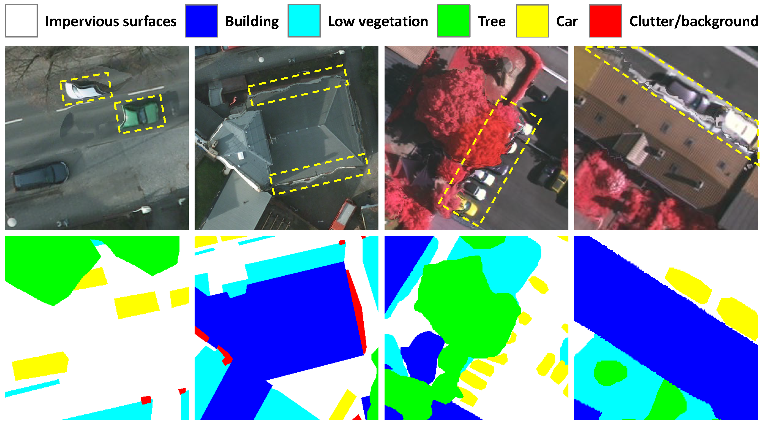
Potsdam dataset (https://www2.isprs.org/commissions/comm2/wg4/benchmark/2d-sem-label-potsdam/ accessed on 29 July 2021): The Potsdam dataset was collected by aerial cameras with a resolution of $6000\times 6000$ pixels over Potsdam City, and the ground sampling distance was 5 cm. The dataset has 38 samples, with 24 for training and 14 for testing. Each sample contains three images with true orthophoto (TOP), digital surface model (DSM), and ground truth, respectively. TOP is composed of three bands of red (R), green (G), and blue (B). DSM consists of the near infrared (NIR) band, which is used to reflect ground height information. Ground truth contains a total of six categories marked in different colors, namely impervious surfaces (white), building (blue), low vegetation (cyan), tree (green), car (yellow), and cluster/background (red).

Vaihingen dataset (https://www2.isprs.org/commissions/comm2/wg4/benchmark/2d-sem-label-vaihingen/ accessed on 29 July 2021): The Vaihingen Dataset presents a relatively small village with many detached buildings, where the defined object categories are the same as the Potsdam dataset. The dataset was collected by an aerial camera with a resolution from $1996\times 1995$ to $3816\times 2550$ pixels. This dataset contains 33 samples, with 16 for training and 17 for testing. Unlike the Potsdam dataset, TOP of Vaihingen consists of NIR, R, and G bands so that TOP may look different from natural images (e.g., vegetation is red). In addition, it also contains the DSM and ground truth of the same number of categories.

Remark: We only use TOP for training without extra DSM information. Due to memory limitations, we cut TOP and ground truth into $512\times 512$ pixels’ patches for training, and use the blending approach in [5] to restore the large mosaics for evaluating. The dataset is divided according to the official recommendations (training:testing = 24:14 on Potsdam and training:testing = 16:17 on Vaihingen). Precision, Recall, F1, Overall accuracy (OA), and mean intersection over union (mIoU) are used to evaluate the accuracy of the model. Furthermore, Floating-Point Operations Per Second (Flops) and Params are used to evaluate the complexity of the model. The aforementioned metrics are as follows.

$$\begin{array}{c}Precision={\displaystyle \frac{TP}{TP+FP}},Recall={\displaystyle \frac{TP}{TP+FN}},F_1=2\times {\displaystyle \frac{Precision\times Recall}{Precision+Recall}}\end{array}$$

(6)

$$\begin{array}{c}OA={\displaystyle \frac{TP+TN}{P+N}},IoU={\displaystyle \frac{TP}{TP+FP+FN}}\end{array}$$

(7)

where $\mathit{T}$, $\mathit{F}$, $\mathit{P}$, and $\mathit{N}$ represent true, false, positive, and negative, respectively. $\mathit{TP}$ denotes the pixels of truly predicted positive class, $\mathit{TN}$ is the truly predicted negative pixels, $\mathit{FP}$ is the falsely predicted positive pixels, and $\mathit{FN}$ is the falsely predicted negative pixels.

4.2. Study for Swin Transformer

Studies have been conducted to explore the potential application of Swin transformer structure in the field of remote sensing image segmentation (on the Potsdam and Vaihingen datasets), including pre-trained weights of Swin transformer, the best input size, the best optimizer, etc. In addition, various segmentation heads have also also compared, including apchead [37], aspphead [16], asppplushead [38], dahead [19], dnlhead [39], fcnhead [6], fpnhead [18], gchead [20], psahead [40], psphead [17], seghead [29], unethead [14], uperhead [30], as well as our proposed mlphead, to evaluate, which head is the most suitable for remote sensing image segmentation tasks. All the experiments below use Swin-B as the baseline and are performed on the Vaihingen dataset without using Testing Time Augmentation (TTA).

4.2.1. Study for Pre-Trained Weights

In this section, the pre-trained weights of Swin transformer on the public datasets are first discussed. To explore the importance of initializing pre-trained weights, we compare different initializing pre-trained weights during the training process, which include without pre-trained weight (w/o), ImageNet 1k (1k means the category numbers) [41], ImageNet 22k, ImageNet 22k to 1k (pre-training on ImageNet 22k and fine tuning on ImageNet 1k), and Ade20k [42].

The pre-trained sizes of $224\times 224$, $384\times 384$ or $512\times 512$ pixels, are meantime discussed. All experiments are performed on the Vaihingen dataset, using $512\times 512$ input size to train 100 epochs, and using Swin transformer base (Swin-B) as the baseline. Swin-B has two model scales, which are large shifted windows size 12 (w12) and small shifted windows size 7 (w7).

In this study, mIoU is selected as the main reference metric to be compared. As is shown in

Table 2. Study for the pre-trained weights on Vaihingen dataset.

Pre-Trained Weight	Pre-Trained Size	Windows Size	Epoch	F1 (%)	OA (%)	mIoU (%)
w/o	/	7	100	81.99	85.58	70.17
	/	7	300	82.85	85.76	71.26
	/	7	1000	83.12	85.83	71.61
ImageNet 1k [41]	224 × 224	7	100	86.23	87.60	76.11
	384 × 384	12	100	86.25	87.68	76.11
ImageNet 22k [41]	224 × 224	7	100	86.63	88.01	76.75
	384 × 384	12	100	86.58	88.04	76.68
ImageNet 22k to 1k [41]	224 × 224	7	100	86.64	87.94	76.73
	384 × 384	12	100	86.47	87.91	76.49
Ade20k [42]	512 × 512	7	100	86.16	87.59	76.03
Potsdam	512 × 512	7	100	82.32	86.70	71.56

, the following results can be concluded. First, the pre-trained weight is very helpful to improve the accuracy of the model, where the model with pre-trained weights obtained an increase of almost 6% on mIoU compared with w/o. Second, it is difficult for the model w/o pre-trained weights to improve the model accuracy even if the training epoch increases from 100 to 1000.

Third, the ImageNet 22k pre-trained dataset is better than other pre-trained datasets (OA in bold). Fourth, the $224\times 224$ pre-trained size is better than $384\times 384$ pre-trained size in performance and computational complexity. Fifth, the pre-trained weight on segmentation dataset Ade20k is not better than the classification dataset ImageNet 22k, because the training data of the Ade20k dataset is much less than ImageNet 22k.

Therefore, large scale pre-training determines the segmentation performance rather than the type of pre-training dataset. Finally, although the mIoU score of using the small-scale remote sensing dataset Potsdam is not good, there is still a significant improvement in comparison with w/o using pre-trained weights (mIoU increased from 70.17% to 71.56%.)

The training size is fixed to $512\times 512$ during the training process; however, the pre-trained weight is obtained with size $224\times 224$ or $384\times 384$, which may affect the final accuracy. Therefore, we further explore the impact on model accuracy when training with different training sizes and pre-trained sizes. The experimental results are shown in

Table 3. Study for the training size on Vaihingen dataset.

Pre-Trained Weight	Pre-Trained Size	Training Size	Windows Size	F1 (%)	OA (%)	mIoU (%)
ImageNet 22k [41]	224 × 224	224 × 224	7	85.98	87.37	75.72
	224 × 224	512 × 512	7	86.63	88.01	76.75
	224 × 224	768 × 768	7	86.66	88.23	76.81
	384 × 384	384 × 384	12	86.47	87.98	76.49
	384 × 384	512 × 512	12	86.58	88.04	76.68

. It can be seen that with a larger training size, the accuracy will obtain an increase because the larger training size provides a larger receptive field.

However, due to memory limitations, it is better to use $512\times 512$ for the complexity-accuracy trade-off. Moreover, when the pre-trained size and training size maintain the same resolution, the OA of the model does not significantly improve, and thus the training size is still the main reason for determining the accuracy of the model. The following experiments will use the current complexity-accuracy trade-off configuration with ImageNet 22k pre-trained weight, $512\times 512$ training size and Swin-B w7 model.

4.2.2. Study for Optimizer

The optimizer plays a paramount role part in deep learning models, directly determining the optimization direction and final performance of the model [43]. Commonly used optimizers in semantic segmentation are SGD [44] and AdamW [45]. SGD is a commonly used optimizer for CNN models, to ensure stable convergence of the model leading to a good convergence performance. AdamW is considered because it has a faster convergence rate than SGD; however, the training process is unstable and heavily depends on the appropriate weight decay and L2 normalization parameters. As a result, AdamW is usually used in the transformer structure with a slower convergence to speed up the model convergence.

The Vision transformer (ViT) model is considered sensitive to the choice of the optimizer (AdamW or SGD); however, it is unknown whether the Swin transformer is also sensitive to the type of optimizers. Therefore, a comparative study was conducted to evaluate the performance of using SGD and AdamW on the Swin transformer structure. It can be seen from

Table 4. The results of optimizers ablation study.

Method	Optimizer	Aux	F1 (%)	OA (%)	mIoU (%)
Swin-B [10]	AdamW [45]	w	86.63	88.01	76.75
	AdamW [45]	w/o	86.18	87.55	76.00
	SGD [44]	w	85.77	87.73	75.52
	SGD [44]	w/o	85.40	87.66	75.00

that AdamW performs better than SGD, and the mIoU can increase by more than 1% by replacing the optimizer.

In addition, when the auxiliary segmentation head (Aux) is added (w for with segmentation head and w/o for no segmentation head), the mIoU can be further increased by about 0.4%. This shows that the Swin transformer still relies on the optimizer selection, and the AdamW optimizer can achieve better performance. As is shown in Figure 11, the AdamW optimizer has a faster convergence rate and lower loss than SGD, which yields the superiority of AdamW being applied in the Swin transformer.

4.2.3. Study for Segmentation Head

The segmentation head determines the utilized degree of features extracted from the backbone, which is a crucial factor to obtain a good segmentation result. After the backbone extracting the features, the segmentation head restores these features to the input image size and finally discriminates categories pixel by pixel. Therefore, a powerful segmentation head is highly important to realize the full performance of the backbone. To this end, we compare dozens of commonly used segmentation heads to explore what kind of head can better achieve the performance based on Swin transformer backbone. The Swin transformer has four output features, named C1, C2, C3 and C4, with corresponding resolutions of $\frac{H}{4}\times \frac{W}{4}$, $\frac{H}{8}\times \frac{W}{8}$, $\frac{H}{16}\times \frac{W}{16}$, and $\frac{H}{32}\times \frac{W}{32}$. The semantic information contained in these features is gradually increased, and the spatial information is gradually decreased.

By observing the number of input layers in

Table 5. The results of Swin-B with different segmentation head on the Vaihingen dataset.

Head	Input Layers	F1 (%)	OA (%)	mIoU (%)	Flops (G)	Params (M)
apchead [37]	C4	82.32	86.70	71.06	93.01	109.47
aspphead [16]	C4	81.39	86.28	69.84	89.26	91.96
asppplushead [38]	C1, C4	86.46	87.92	76.47	111.03	93.14
dahead [19]	C4	82.27	86.66	70.96	89.85	93.91
dnlhead [39]	C4	82.34	86.67	71.07	90.24	95.54
fpnhead [18]	C1, C2, C3, C4	86.51	87.92	76.56	179.99	97.01
fcnhead [6]	C4	82.34	86.69	71.06	90.07	95.01
gchead [20]	C4	82.19	86.60	70.86	90.08	95.14
psahead [40]	C4	82.22	86.69	70.95	90.86	97.99
psphead [17]	C4	82.15	86.55	70.80	89.49	93.70
seghead [29]	C1, C2, C3, C4	86.39	87.84	76.38	97.20	90.41
unethead [14]	C1, C2, C3, C4	86.35	87.85	76.33	153.81	89.84
uperhead [30]	C1, C2, C3, C4	86.63	88.01	76.75	299.42	121.17
mlphead	C1, C2, C3, C4	86.38	87.90	76.37	95.22	88.89

, the head using at least two input layers obviously has a higher accuracy (mIoU over 76%). In comparison with aspphead, asppplushead integrates shallow features C1 so that the mIoU improves 6.63%, meaning that integrated features at different scales is essential to improve the final performance. In addition, it can be found that when taking only C4 as the input of the segmentation head, such as apchead, dahead, dnlhead, gchead, and psahead, the attention-mechanism-based designs achieve poor performance.

Instead, heads incorporating different scales information, such as asppplushead, fpnhead, seghead, unethead, upperhead, and mlphead, are capable of obtaining good performance. As a result, based on these findings, the proposed mlphead head based on multi-scale fusion can achieve good performance. It is worth noting that the Flops of mlphead are only $\frac{1}{3}$ of the upperhead, and the params is the lowest of all heads.

Further, the impact of different input layers on the final performance is also compared. C1, C2, C3, and C4 are the input sizes of $\frac{H}{4}\times \frac{W}{4}$, $\frac{H}{8}\times \frac{W}{8}$, $\frac{H}{16}\times \frac{W}{16}$, and $\frac{H}{32}\times \frac{W}{32}$, respectively. We use stride 4 (s4), s8, s16, and s32 to represent the multiples of the corresponding downsampling size to correspond to the four input sizes. As is depicted in

Table 6. The results of aspphead and dahead with different input layers.

Head	Input Layers	Stride	F1 (%)	OA (%)	mIoU (%)	Flops (G)	Params (M)
aspphead [16]	C1	4	77.22	83.35	62.88	80.65	87.99
	C2	8	82.82	85.57	71.21	80.64	88.18
	C3	16	85.59	87.74	75.29	80.63	88.94
	C4	32	81.39	86.28	69.84	89.26	91.96
dahead [19]	C1	4	79.76	83.32	66.92	90.88	88.02
	C2	8	83.83	85.92	72.51	82.41	88.30
	C3	16	85.62	87.70	75.31	81.35	89.42
	C4	32	82.27	86.66	70.96	89.85	93.91

, aspphead and dahead with poor performance are chosen to explore the performance of different input layers. It can be seen that when C1 or C4 is used, the mIoU is low because C1 lacks semantic information and C4 lacks spatial information. When C3 is used, a good balance between spatial information and semantic information can be achieved, but it is still slightly lower than using all four layers. To guarantee lower Flops and Params, C3 can be used as the input of the segmentation head.

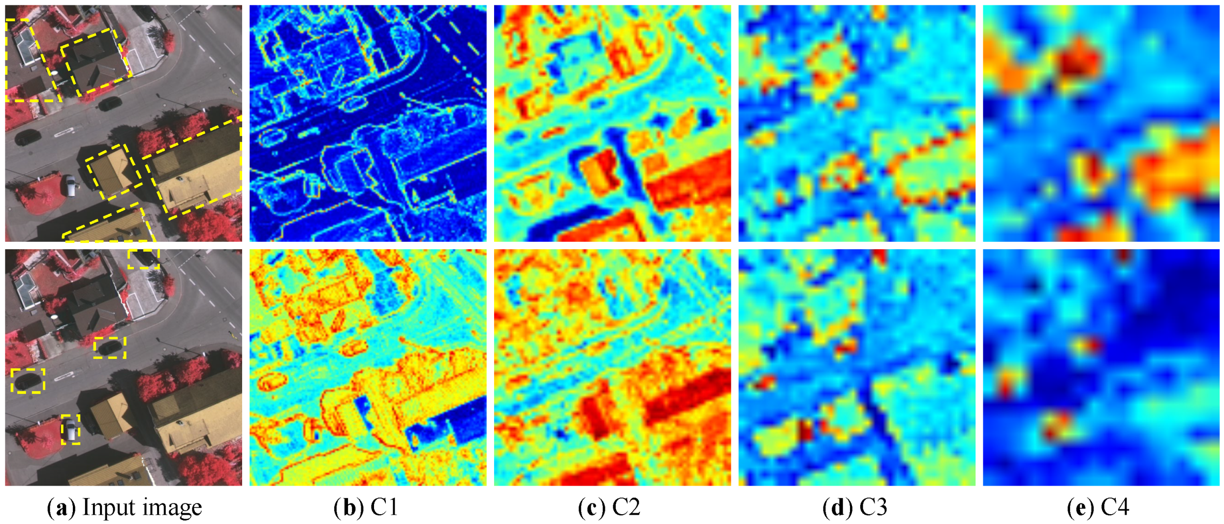
Finally, to intuitively understand the features contained in each layer of input layers, the features of C1, C2, C3, and C4 are visualized in Figure 12, where the red parts indicate the areas of concern. It can be seen from left to right that the buildings (with yellow dashed box) in the image of first row are gradually concerned.

As can be seen, the feature C1 focuses on the edges of all the objects, the feature C2 focuses on the rectangular shape including most of the buildings, the feature C3 only focuses on the edge of buildings, and the feature C4 only focuses the building category, which reveals that the attention of the model is gradually transferred from random categories to specific category (e.g., building category in first low). Moreover, it also explains why the C3 can achieve the best performance among the four layers, since the C3 layer can distinguish different categories while retaining spatial information (e.g., the edge). The category car in the second row also presents the same conclusion.

4.3. Efficient Transformer Backbone and Mlphead

In practical scenarios, the inference speed (usually expressed by processing images per second, abbreviated as img/s) of the model is important to make real-time predictions. When the input image size is fixed, the efficiency of the model mainly depends on the complexity of the model, which is usually related to the Flops and Params. However, the model inference speed is not linearly related to the Flops and Params. Therefore, in this experiment, we introduce the model inference speed evaluation index img/s to evaluate whether the model can complete the video real-time inference requirements. In

Table 7. Inference speed evaluation on Swin-B and Efficinet-B.

Backbone	Head	F1 (%)	OA (%)	mIoU (%)	Flops (G)	Params (M)	Speed (img/s)
Swin-B [10]	uperhead [30]	86.63	88.01	76.75	299.42	121.17	18.9
	mlphead	86.38	87.90	76.37	95.22	88.89	29.8
Efficient-B	uperhead [30]	86.23	87.62	76.09	238.72	61.87	24.7
	mlphead	85.92	87.38	75.61	35.04	31.28	47.9

, we compare the four combinations of the Swin transformer, uperhead, Efficient transformer, and mlphead to evaluate the advantages of Efficient transformer and mlphead in inference speed.

It can be seen from Table 7 that with the same uperhead, comparing Swin-B and Efficient-B, the mIoU of Efficient-B drops by 0.66%, but the inference speed increases to 24.7 img/s, meeting the real-time requirements (usually 25 img/s). When the head is replaced with the lighter mlphead, the inference speed is increased by 2.5 times (47.9 img/s). Therefore, when a small amount of accuracy is sacrificed, the model can meet the requirements of real-time inference, which is of great significance to the practical application of the model and saving computing resources.

4.4. Edge Processing Methods

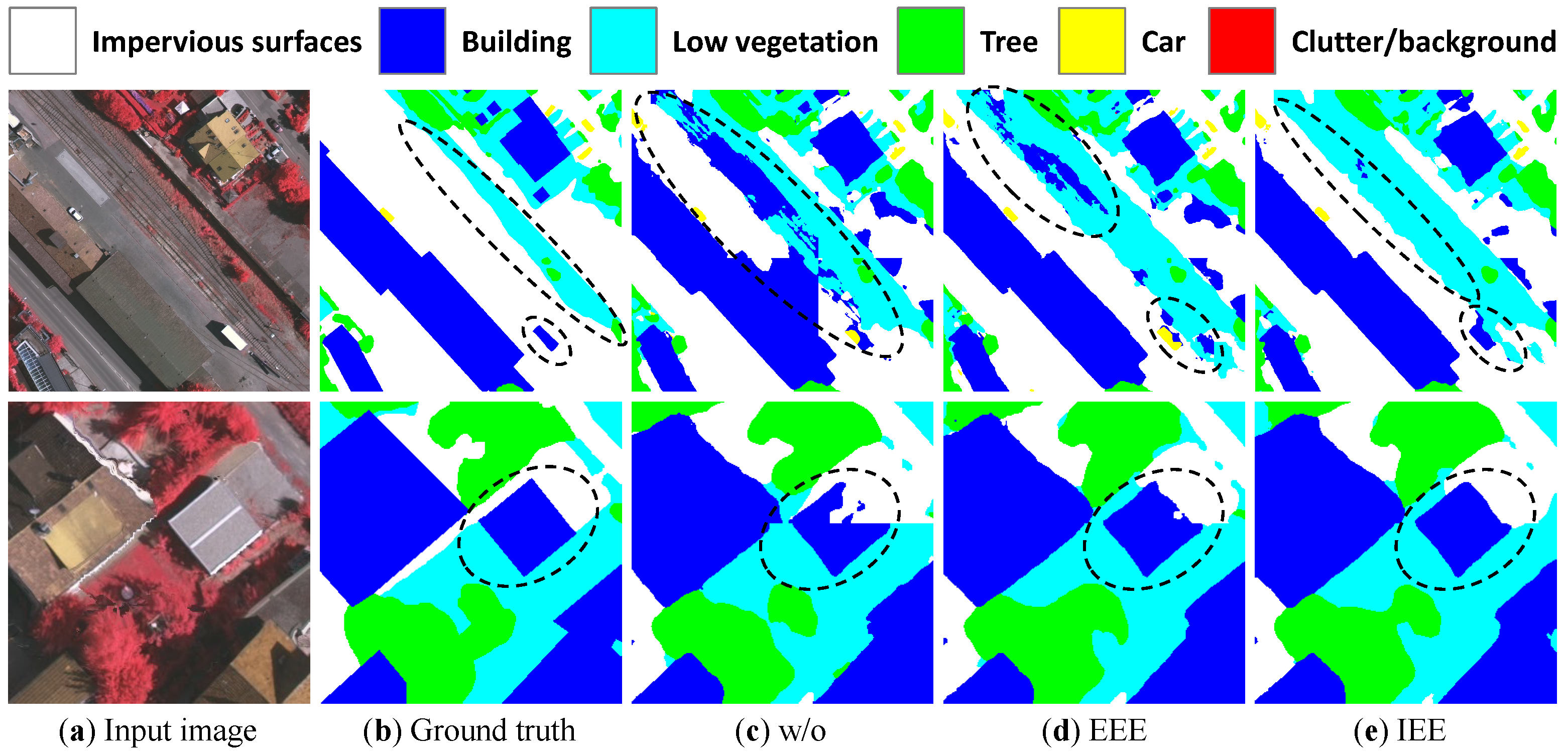
To verify the effectiveness of our proposed explicit edge enhancement (EEE) and implicit edge enhancement (IEE) methods, an ablation experiment is carried out on the Vaihingen dataset based on the Efficient-T with the mlphead model. This can be found in

Table 8. The ablation study of edge processing methods.

Method	IEE		EEE	F1 (%)	OA (%)	mIoU (%)
	ES	EEL	AEF
Efficient-T				85.19	86.90	74.56
	✓			85.30	87.02	74.74
		✓		85.29	86.92	74.69
	✓	✓		85.50	87.25	75.04
			✓	85.20	87.11	74.92
	✓	✓	✓	85.57	87.24	75.15

, the effectiveness of auxiliary edge fusion (AEF), edge supervision (ES), and edge enhancement loss (EEL) methods are evaluated. It can be seen that by using the proposed explicit and implicit edge enhancement methods, the IEE improves the mIoU by 0.48%, the EEE improves the mIoU by 0.36%.

When combining explicit edge enhancement and implicit edge enhancement methods, the final mIoU obtains a 0.59% increase, and it seems that the effects of IEE and EEE are overlapping. We compare the results of adding IEE and EEE methods on the Vaihingen and Potsdam datasets in

Table 9. Results on Vaihingen and Potsdam datasets, “†” means using IEE and EEE methods.

Dataset	Method	Recall (%)	Precision (%)	F1 (%)	OA (%)	mIoU (%)
Vaihingen	Efficient-T	84.84	85.54	85.19	86.90	74.56
	Efficient-T †	85.43	85.71	85.57	87.24	75.15
Potsdam	Efficient-T	89.24	88.62	88.93	88.04	80.35
	Efficient-T †	90.05	89.21	89.63	88.66	81.41

. The mIoU of Potsdam obtains a 1.06% increase, and the Vaihingen mIoU improves 0.59%. As the Potsdam dataset has more complex scenes, the Efficient-T without edge enhancement methods found it more difficult to predict a fine edge, and thus the edge enhancement methods may produce more obvious improvements.

Finally, we also compare the visual effects of employing the explicit edge enhancement and implicit edge enhancement methods. Figure 13 shows the improvements in the edge part, where the edge of without (w/o) any edge processing methods is irregular and wrongly classified (see ellipse). Using EEE or IEE can obtain a sharper edge, especially by employing the IEE method, the edge improves a great deal.

4.5. Comparison to SOTA Methods

Previous experiments have deeply discussed the application of the Swin transformer in remote sensing tasks and verified our proposed Efficient transformer, mlphead, and edge enhancement methods. In this section, based on our previous experimental configuration and the same parameter settings, we compare some classic CNN models, including FCN [6], FPN [18], PSPNet [17], UNet [14], BiseNet_v2 [23], DeepLab_v3 [16], and DANet [19], as well as the Swin transformer studied in this article. The Efficient transformer with mlphead model, including Efficient-T, Efficient-S, Efficient-B, and Efficient-L are compared.

We evaluate the accuracy and complexity of the model on the Vaihingen and Potsdam datasets. For a fair comparison, the CNN models all use ImageNet 1k pre-trained weights to initialize the models, and all models are with no Testing Time Augmentation (TTA). On the Potsdam dataset, to avoid the overfitting problem, we add a mixup data augmentation strategy.

Results on Vaihingen: As can be seen from

Table 10. Comparison of SOTA methods on the Vaihingen dataset.

Method	Recall (%)	Precision (%)	F1 (%)	OA (%)	mIoU (%)	Flops (G)	Params (M)
FCN [6]	79.03	80.84	79.92	84.41	67.58	80.34	15.31
FPN [18]	79.65	85.06	82.26	85.60	69.95	47.00	27.71
PSPNet [17]	85.27	86.40	85.83	87.27	75.47	177.38	48.63
UNet [14]	83.12	84.16	83.64	85.95	72.33	124.12	13.40
BiseNet_v2 [23]	77.06	80.96	78.96	83.83	66.05	12.92	3.63
DeepLab_v3 [16]	85.25	86.51	85.88	87.34	75.54	163.86	41.68
DANet [19]	85.12	86.29	85.70	87.20	75.29	209.76	49.49
Swin-T [10]	85.90	86.53	86.21	87.69	76.09	236.90	59.83
Swin-S [10]	86.01	86.68	86.35	87.70	76.29	260.66	81.15
Swin-B [10]	86.50	86.77	86.63	88.01	76.75	299.42	121.17
Swin-L [10]	86.58${}_{+1.33}$	86.96${}_{+0.45}$	86.77${}_{+0.89}$	88.14${}_{+0.80}$	76.97${}_{+1.43}$	408.75	233.65
Efficient-T	85.43	85.71	85.57	87.24	75.15	16.78	11.30
Efficient-S	85.21	86.03	85.62	87.20	75.17	20.18	14.47
Efficient-B	85.38	86.46	85.92	87.38	75.61	35.04	31.28
Efficient-L	$85.63{}_{+0.38}$	$86.58{}_{+0.07}$	86.10${}_{+0.22}$	87.56${}_{+0.22}$	75.92${}_{+0.38}$	56.64	52.63

, in comparison with DeepLab_v3, Swin-L obtains an improvement of 1.33%, 0.45%, 0.89%, 0.80%, and 1.43% on Recall, Precision, F1, OA, and mIoU, respectively. However, the shortcomings of Swin-L are also obvious. For instance, the cost of Flops and Params is 2.5 times and 5.6 times of DeepLab_v3. On the contrary, our proposed Efficient-L model costs fewer calculations. Compared with DeepLab_v3, it obtains an improvement of 0.38%, 0.07%, 0.22%, 0.22%, and 0.38% on Recall, Precision, F1, OA, and mIoU, respectively, but only $\frac{1}{3}$ of the Flops and 1.3 times the Params are used.

Moreover, the Efficient-T model only uses 16.78G Flops and 11.30M Params, which is almost equivalent to BiseNet_v2, but mIoU improved by 9.1%. Therefore, it can be concluded that the Efficient transformer model is better than the CNN model in terms of the accuracy and complexity, and although the Swin transformer is far better than the CNN model in terms of accuracy, the excessive complexity may be a major problem.

Results on Potsdam: As can be seen from

Table 11. Comparison of SOTA methods on the Potsdam dataset.

Method	Recall (%)	Precision (%)	F1 (%)	OA (%)	mIoU (%)	Flops (G)	Params (M)
FCN [6]	86.24	85.54	85.89	85.30	75.37	80.34	15.31
FPN [18]	85.67	88.06	86.85	86.16	76.38	47.00	27.71
PSPNet [17]	90.06	89.35	89.70	88.75	81.52	177.38	48.63
UNet [14]	88.86	88.18	88.52	87.13	79.52	124.12	13.40
BiseNet_v2 [23]	82.92	81.12	82.01	81.02	69.65	12.92	3.63
DeepLab_v3 [16]	90.31	89.59	89.95	88.85	81.92	163.86	41.68
DANet [19]	90.29	89.65	89.97	89.00	81.96	209.76	49.49
Swin-T [10]	90.93	89.95	90.44	89.39	82.73	236.90	59.83
Swin-S [10]	90.98	90.05	90.51	89.47	82.84	260.66	81.15
Swin-B [10]	91.10	90.06	90.58	89.46	82.95	299.42	121.17
Swin-L [10]	91.26${}_{+0.97}$	90.19${}_{+0.54}$	90.72${}_{+0.75}$	89.65${}_{+0.65}$	83.22${}_{+1.26}$	408.75	233.65
Efficient-T	90.05	89.21	89.63	88.66	81.41	16.78	11.30
Efficient-S	90.42	89.48	89.95	89.05	81.93	20.18	14.47
Efficient-B	90.70	89.69	90.19	89.25	82.34	35.04	31.28
Efficient-L	90.89${}_{+0.60}$	89.92${}_{+0.27}$	90.40${}_{+0.43}$	89.44${}_{+0.44}$	82.68${}_{+0.72}$	56.64	52.63

, compared to DANet, the best-performing CNN model on the Potsdam dataset, Swin-L obtains 0.97%, 0.54%, 0.75%, 0.65%, and 1.26% improvements on Recall, Precision, F1, OA, and mIoU, respectively. Efficient-L gains 0.6%, 0.27%, 0.43%, 0.44%, and 0.72% improvements on Recall, Precision, F1, OA, and mIoU, respectively. It can be found that on the Potsdam dataset, Efficient-L achieves a performance closer to Swin-L, and the scores of Swin-T, Swin-S, Swin-B, and Swin-L are also closer, which indicates that the Efficient transformer can obtain greater benefits on large scale datasets.

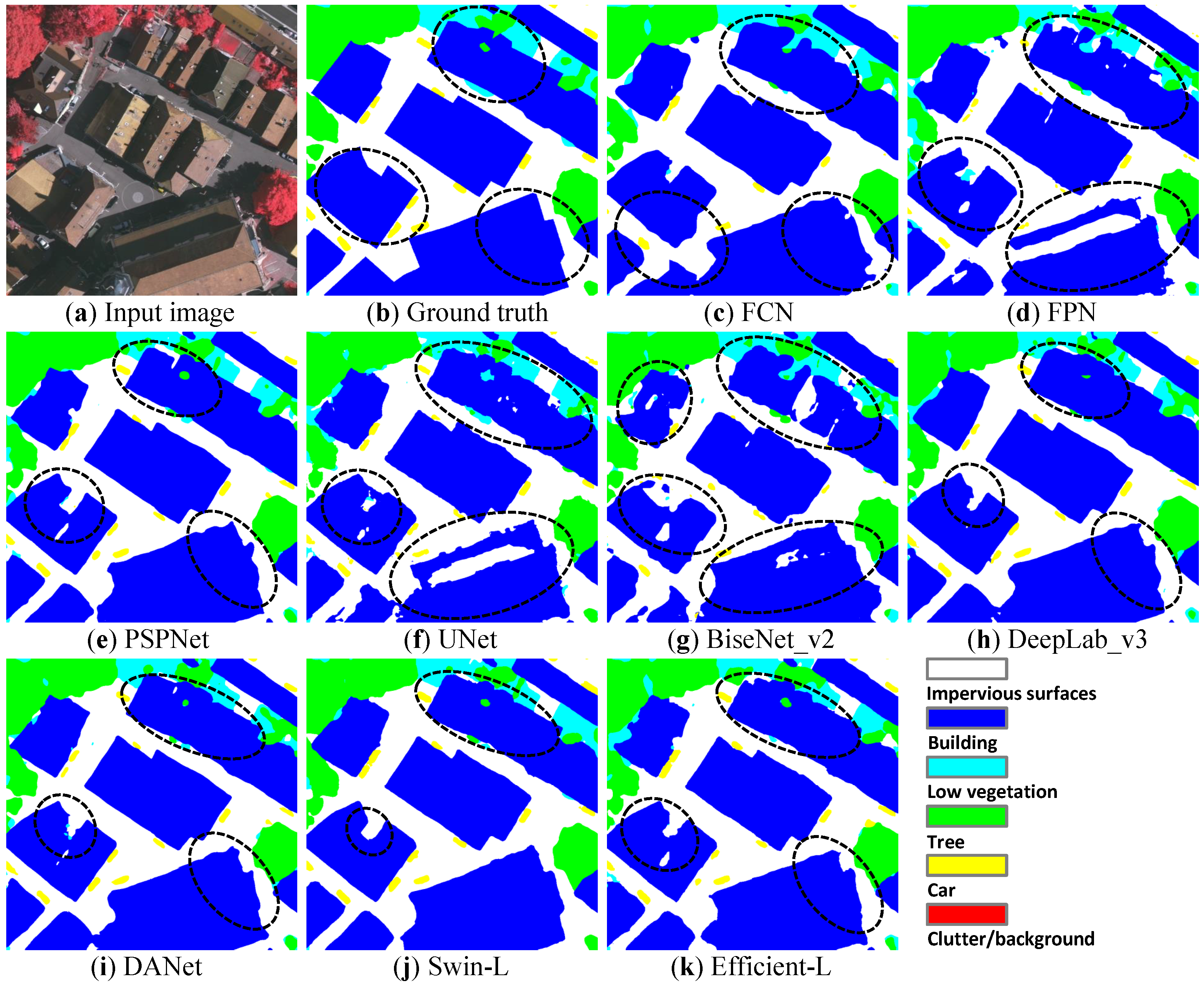
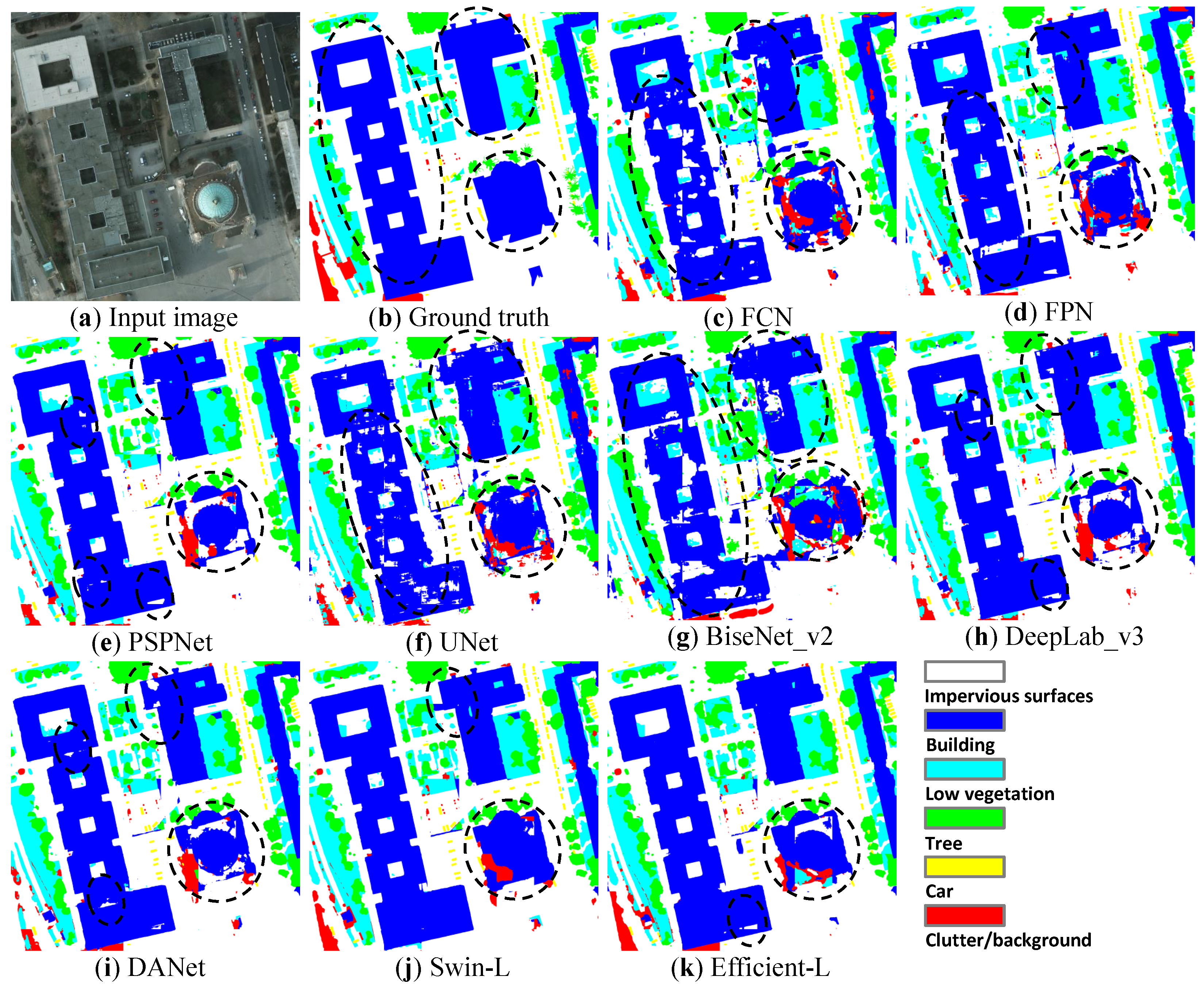
In addition, from the prediction maps of Figure 14 and Figure 15, the transformer models can clearly achieve better segmentation results on large scale objects (e.g., buildings) compared with the CNN models, which are attributed to the global relation modeling ability of transformers.

5. Discussion

To exploit the large differences between transformer-based methods and the CNN-based methods, a comparative study on the Vaihingen and Potsdam datasets was conducted. For a fair comparison, both methods use Testing Time Augmentation (TTA), including flip and multi-scale testing. Flip includes horizontal mirror flip and vertical mirror flip, and the ratio of multi-scale testing is set as 0.5, 0.75, 1.0, 1.25, and 1.5. The methods for comparison include three CNN methods, which were the top 1 method on the Vaihingen challenge called HUSTW5, the top 1 method on the Potsdam challenge called SWJ_2 [46], and a previous SOTA work HRCNet_W48 [5], and the two transformer-based methods proposed in this article, namely Swin-L with uperhead, Efficient-L with mlphead.

The results are shown in

Table 12. Comparison to Top 1 methods on the Vaihingen and Potsdam datasets.

Dataset	Method	Recall (%)	Precision (%)	F1 (%)	OA (%)	mIoU (%)
Vaihingen	HUSTW5	83.32	86.20	84.50	88.60	/
	HRCNet_W48 [5]	86.29	86.47	86.07	88.56	74.11
	Swin-L [10]	87.29${}_{+1.00}$	87.97${}_{+1.50}$	87.60${}_{+1.53}$	88.85${}_{+0.29}$	78.26${}_{+4.15}$
	Efficient-L	86.29	87.89${}_{+1.42}$	87.01${}_{+0.94}$	88.41	77.34${}_{+3.23}$
Potsdam	SWJ_2 [46]	89.40	89.82	89.58	89.40	/
	HRCNet_W48 [5]	90.69	89.90	90.20	89.50	81.20
	Swin-L [10]	91.38${}_{+0.69}$	90.61${}_{+0.71}$	90.94${}_{+0.74}$	90.02${}_{+0.52}$	83.60${}_{+2.4}$
	Efficient-L	91.52${}_{+0.83}$	90.49${}_{+0.59}$	90.99${}_{+0.79}$	90.08${}_{+0.58}$	83.66${}_{+2.46}$

. First, observing the results on the Vaihingen dataset, it can be found that transformer-based methods were significantly better than the CNN methods in most of the accuracy metrics by taking HRCNet_W48 as the benchmark. On the Potsdam dataset, Efficient-L and Swin-L also easily outperformed the CNN-based methods in all the accuracy metrics. When using the same TTA strategy, Efficient-L outperformed Swin-L on mIoU, presenting that Efficient-L can obtain higher benefits from TTA.

Then, by observing the results of OA and mIoU, it is found that transformer-based methods had less improvement in OA value but a larger increase in mIoU. The OA metric is used to describe the correctly classified proportion of pixels in the classification of a picture, mIoU describes the degree of overlap between two regions. Therefore, when the OA is approximately the same, the method with high mIoU has higher prediction accuracy.

Then, we calculate the IoU of each category. The comparison results are shown in

Table 13. IoU scores of each category on the Vaihingen and Potsdam datasets.

Dataset	Method	Imp Surf	Building	Low Veg	Tree	Car	mIoU (%)
Vaihingen	HRCNet_W48 [5]	81.05	86.65	66.91	76.63	59.31	74.11
	Swin-L [10]	83.35${}_{+2.30}$	89.86${}_{+3.21}$	69.45${}_{+2.54}$	77.63 ${}_{+1.00}$	71.02 ${}_{+11.71}$	78.26 ${}_{+4.15}$
	Efficient-L	82.75${}_{+1.70}$	88.75 ${}_{+2.10}$	68.66${}_{+1.75}$	77.32 ${}_{+0.69}$	69.24 ${}_{+9.93}$	77.34 ${}_{+3.23}$
Potsdam	HRCNet_W48 [5]	83.58	91.15	73.07	74.88	83.32	81.20
	Swin-L [10]	86.13${}_{+2.55}$	93.21${}_{+2.06}$	76.08${}_{+3.01}$	76.75${}_{+1.87}$	85.85${}_{+2.53}$	83.60${}_{+2.4}$
	Efficient-L	85.82${}_{+2.24}$	93.09${}_{+1.94}$	76.38${}_{+3.31}$	78.02${}_{+3.14}$	85.01${}_{+1.69}$	83.66${}_{+2.46}$

. On the Vaihingen dataset, the IoU of the Car category has significantly improved owing to cascade addition architecture in the segmentation head, improving the ability to recognize small objects. In addition, the use of large scale pre-trained weights makes it possible to achieve good classification performance even on the small scale dataset of Vaihingen when the proportion of car category is very low.

On the Potsdam dataset, since the data of each category is sufficient, the improvement effect of each category is relatively close. Efficient-L and Swin-L have a significant improvement in the low vegetation category, showing that the transformer structure has an advantage in dealing with large scale irregular categories, which is attributed to the establishment of global relations.

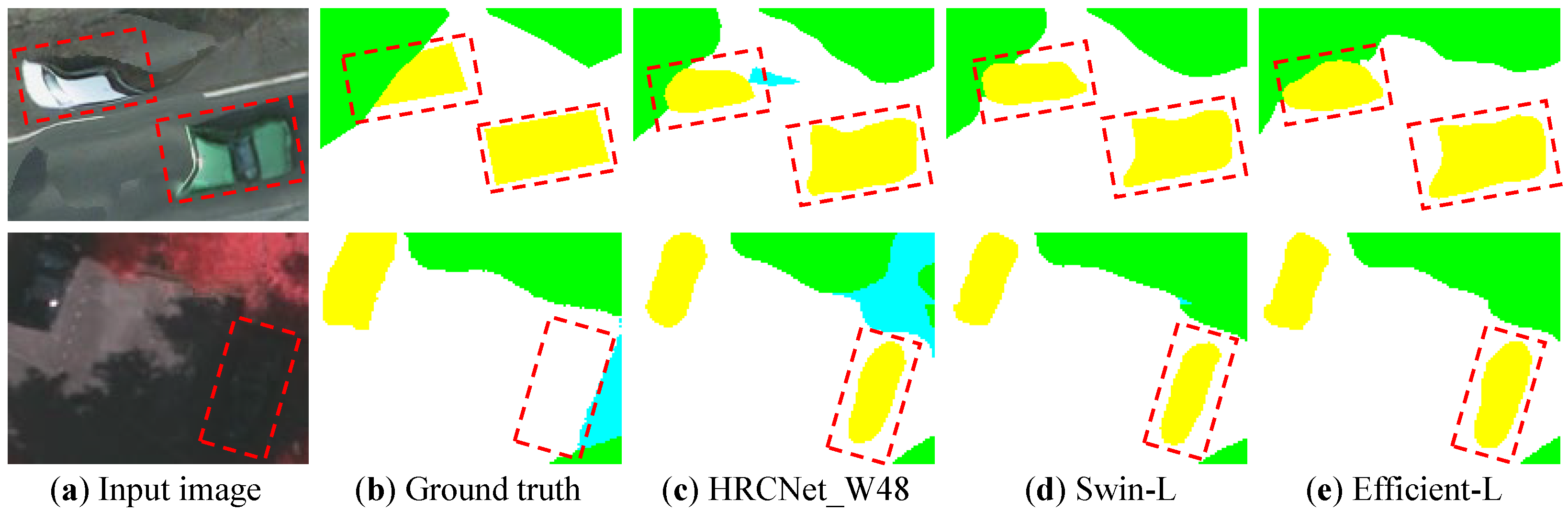
In Figure 16, we compare different methods when dealing with blurry areas. The top image displays blurry areas of the cars, and the bottom image shows the missing target in the ground truth. The transformer-based methods (Swin-L and Efficient-L) tend to predict better edges of blurry areas, which are close to the input image, instead of the revised ground truth. HRCNet_W48 is slightly weak at dealing with blurry input, even making wrong predictions (blue pixels). As for the imperceptible objects in the shadow, all the compared deep learning methods can correctly identify the objects.

6. Conclusions

In this paper, the hierarchical Swin transformer was introduced, and we first attempted to deal with remote sensing image semantic segmentation. Based on that, a novel transformer was proposed to cope with high computation loads and blurry edge problems. In particular, we first propose a novel segmentation model composing of Efficient transformer and mlphead to reduce the computation load. The Efficient transformer has a lower computational complexity but competitive performance to the Swin transformer, and mlphead is a pure transformer design enabling acceleration of the inference speed.

Composing the two lightweight designs, the Efficient transformer (e.g., Efficient-B, see Table 7) achieved 47.9 img/s inference speed with $512\times 512$ pixels input, greatly outperforming the real-time inference speed of 25 img/s. In addition, explicit and implicit enhancement methods are well designed to improve the edge segmentation. By using the two edge enhancement methods, the original blurry edge can be significantly improved. Finally, the proposed Efficient transformer was compared with state-of-the-art models and achieved a tremendous improvement where Efficient-L achieved 77.34% and 83.66% on mIoU scores on the Vaihingen and Potsdam datasets, respectively.

In comparison with previous SOTA works HRCNet_48, Efficient-L obtained a 3.23% mIoU improvement on Vaihingen and 2.46% mIoU improvement on Potsdam. In the future, a better edge extractor in the explicit enhancement method is desired to further promote remote sensing segmentation performance.

References

1. Witharana, C.; Bhuiyan, M.A.E.; Liljedahl, A.K.; Kanevskiy, M.; Epstein, H.E.; Jones, B.M.; Daanen, R.; Griffin, C.G.; Kent, K.; Jones, M.K.W. Understanding the synergies of deep learning and data fusion of multispectral and panchromatic high resolution commercial satellite imagery for automated ice-wedge polygon detection. ISPRS J. Photogramm. Remote Sens. 2020, 170, 174–191. [Google Scholar] [CrossRef]
2. Zhang, T.; Su, J.; Liu, C.; Chen, W.H. State and parameter estimation of the AquaCrop model for winter wheat using sensitivity informed particle filter. Comput. Electron. Agric. 2021, 180, 105909. [Google Scholar] [CrossRef]
3. Zhang, J.; Lin, S.; Ding, L.; Bruzzone, L. Multi-Scale Context Aggregation for Semantic Segmentation of Remote Sensing Images. Remote Sens. 2020, 12, 701. [Google Scholar] [CrossRef] [Green Version]
4. Khan, S.; Naseer, M.; Hayat, M.; Zamir, S.W.; Khan, F.S.; Shah, M. Transformers in vision: A survey. arXiv 2021, arXiv:2101.01169. [Google Scholar]
5. Xu, Z.; Zhang, W.; Zhang, T.; Li, J. HRCNet: High-resolution context extraction network for semantic segmentation of remote sensing images. Remote Sens. 2021, 13, 71. [Google Scholar] [CrossRef]
6. Long, J.; Shelhamer, E.; Darrell, T. Fully convolutional networks for semantic segmentation. In Proceedings of the IEEE Conference on Computer Vision and Pattern Recognition, Boston, MA, USA, 7–12 June 2015; pp. 3431–3440. [Google Scholar]
7. Vaswani, A.; Shazeer, N.; Parmar, N.; Uszkoreit, J.; Jones, L.; Gomez, A.N.; Kaiser, Ł.; Polosukhin, I. Attention is all you need. arXiv 2017, arXiv:1706.03762. [Google Scholar]
8. Dosovitskiy, A.; Beyer, L.; Kolesnikov, A.; Weissenborn, D.; Zhai, X.; Unterthiner, T.; Dehghani, M.; Minderer, M.; Heigold, G.; Gelly, S.; et al. An image is worth 16x16 words: Transformers for image recognition at scale. arXiv 2020, arXiv:2010.11929. [Google Scholar]
9. Zheng, S.; Lu, J.; Zhao, H.; Zhu, X.; Luo, Z.; Wang, Y.; Fu, Y.; Feng, J.; Xiang, T.; Torr, P.H.; et al. Rethinking semantic segmentation from a sequence-to-sequence perspective with transformers. In Proceedings of the IEEE/CVF Conference on Computer Vision and Pattern Recognition, Nashville, TN, USA, 19–25 June 2021; pp. 6881–6890. [Google Scholar]
10. Liu, Z.; Lin, Y.; Cao, Y.; Hu, H.; Wei, Y.; Zhang, Z.; Lin, S.; Guo, B. Swin transformer: Hierarchical vision transformer using shifted windows. arXiv 2021, arXiv:2103.14030. [Google Scholar]
11. Zhang, Q.; Yang, Y. ResT: An Efficient Transformer for Visual Recognition. arXiv 2021, arXiv:2105.13677. [Google Scholar]
12. Tolstikhin, I.; Houlsby, N.; Kolesnikov, A.; Beyer, L.; Zhai, X.; Unterthiner, T.; Yung, J.; Keysers, D.; Uszkoreit, J.; Lucic, M.; et al. Mlp-mixer: An all-mlp architecture for vision. arXiv 2021, arXiv:2105.01601. [Google Scholar]
13. Chu, X.; Tian, Z.; Wang, Y.; Zhang, B.; Ren, H.; Wei, X.; Xia, H.; Shen, C. Twins: Revisiting the design of spatial attention in vision transformers. arXiv 2021, arXiv:2104.13840. [Google Scholar]
14. Ronneberger, O.; Fischer, P.; Brox, T. U-net: Convolutional Networks for Biomedical Image Segmentation. In Proceedings of the International Conference on Medical Image Computing And Computer-Assisted Intervention, Munich, Germany, 5–9 October 2015; pp. 234–241. [Google Scholar]
15. Jin, Y.; Xu, W.; Zhang, C.; Luo, X.; Jia, H. Boundary-aware refined network for automatic building extraction in very high-resolution urban aerial images. Remote Sens. 2021, 13, 692. [Google Scholar] [CrossRef]
16. Chen, L.C.; Papandreou, G.; Schroff, F.; Adam, H. Rethinking atrous convolution for semantic image segmentation. arXiv 2017, arXiv:1706.05587. [Google Scholar]
17. Zhao, H.; Shi, J.; Qi, X.; Wang, X.; Jia, J. Pyramid scene parsing network. In Proceedings of the IEEE Conference on Computer Vision and Pattern Recognition, Honolulu, HI, USA, 21–26 July 2017; pp. 2881–2890. [Google Scholar]
18. Lin, T.Y.; Dollár, P.; Girshick, R.; He, K.; Hariharan, B.; Belongie, S. Feature pyramid networks for object detection. In Proceedings of the IEEE Conference on Computer Vision and Pattern Recognition, Honolulu, HI, USA, 21–26 July 2017; pp. 2117–2125. [Google Scholar]
19. Fu, J.; Liu, J.; Tian, H.; Li, Y.; Bao, Y.; Fang, Z.; Lu, H. Dual attention network for scene segmentation. In Proceedings of the IEEE Conference on Computer Vision and Pattern Recognition, Long Beach, CA, USA, 16–20 June 2019; pp. 3146–3154. [Google Scholar]
20. Cao, Y.; Xu, J.; Lin, S.; Wei, F.; Hu, H. Gcnet: Non-local networks meet squeeze-excitation networks and beyond. In Proceedings of the IEEE International Conference on Computer Vision Workshops, Seoul, Korea, 27 October–2 November 2019. [Google Scholar]
21. Hu, J.; Shen, L.; Sun, G. Squeeze-and-excitation networks. In Proceedings of the IEEE Conference on Computer Vision and Pattern Recognition, Salt Lake City, UT, USA, 18–22 June 2018; pp. 7132–7141. [Google Scholar]
22. Yu, C.; Wang, J.; Peng, C.; Gao, C.; Yu, G.; Sang, N. Bisenet: Bilateral segmentation network for real-time semantic segmentation. In Proceedings of the European Conference on Computer Cision (ECCV), Munich, Germany, 8–14 September 2018; pp. 325–341. [Google Scholar]
23. Yu, C.; Gao, C.; Wang, J.; Yu, G.; Shen, C.; Sang, N. BiSeNet V2: Bilateral Network with Guided Aggregation for Real-time Semantic Segmentation. arXiv 2020, arXiv:2004.02147. [Google Scholar]
24. Howard, A.G.; Zhu, M.; Chen, B.; Kalenichenko, D.; Wang, W.; Weyand, T.; Andreetto, M.; Adam, H. Mobilenets: Efficient convolutional neural networks for mobile vision applications. arXiv 2017, arXiv:1704.04861. [Google Scholar]
25. Sandler, M.; Howard, A.; Zhu, M.; Zhmoginov, A.; Chen, L.C. Mobilenetv2: Inverted residuals and linear bottlenecks. In Proceedings of the IEEE Conference on Computer Vision and Pattern Recognition, Salt Lake City, UT, USA, 18–22 June 2018; pp. 4510–4520. [Google Scholar]
26. Chen, J.; Lu, Y.; Yu, Q.; Luo, X.; Adeli, E.; Wang, Y.; Lu, L.; Yuille, A.L.; Zhou, Y. Transunet: Transformers make strong encoders for medical image segmentation. arXiv 2021, arXiv:2102.04306. [Google Scholar]
27. Xie, E.; Wang, W.; Yu, Z.; Anandkumar, A.; Alvarez, J.M.; Luo, P. SegFormer: Simple and Efficient Design for Semantic Segmentation with Transformers. arXiv 2021, arXiv:2105.15203. [Google Scholar]
28. Yang, G.; Zhang, Q.; Zhang, G. EANet: Edge-Aware Network for the Extraction of Buildings from Aerial Images. Remote Sens. 2020, 12, 2161. [Google Scholar] [CrossRef]
29. Sun, K.; Zhao, Y.; Jiang, B.; Cheng, T.; Xiao, B.; Liu, D.; Mu, Y.; Wang, X.; Liu, W.; Wang, J. High-resolution representations for labeling pixels and regions. arXiv 2019, arXiv:1904.04514. [Google Scholar]
30. Xiao, T.; Liu, Y.; Zhou, B.; Jiang, Y.; Sun, J. Unified perceptual parsing for scene understanding. In Proceedings of the European Conference on Computer Vision (ECCV), Munich, Germany, 8–14 September 2018; pp. 418–434. [Google Scholar]
31. Haut, J.M.; Bernabé, S.; Paoletti, M.E.; Fernandez-Beltran, R.; Plaza, A.; Plaza, J. Low–high-power consumption architectures for deep-learning models applied to hyperspectral image classification. IEEE Geosci. Remote Sens. Lett. 2018, 16, 776–780. [Google Scholar] [CrossRef]
32. Zhang, C.; Jiang, W.; Zhao, Q. Semantic Segmentation of Aerial Imagery via Split-Attention Networks with Disentangled Nonlocal and Edge Supervision. Remote Sens. 2021, 13, 1176. [Google Scholar] [CrossRef]
33. Zhang, T.; Su, J.; Xu, Z.; Luo, Y.; Li, J. Sentinel-2 satellite imagery for urban land cover classification by optimized random forest classifier. Appl. Sci. 2021, 11, 543. [Google Scholar] [CrossRef]
34. Yuan, W.; Zhang, W.; Lai, Z.; Zhang, J. Extraction of Yardang characteristics using object-based image analysis and canny edge detection methods. Remote Sens. 2020, 12, 726. [Google Scholar] [CrossRef] [Green Version]
35. He, K.; Zhang, X.; Ren, S.; Sun, J. Deep residual learning for image recognition. In Proceedings of the IEEE Conference on Computer Vision and Pattern Recognition, Las Vegas, NV, USA, 27–30 June 2016; pp. 770–778. [Google Scholar]
36. Sugano, H.; Miyamoto, R. Parallel implementation of morphological processing on cell/BE with OpenCV interface. In Proceedings of the 2008 3rd International Symposium on Communications, Control and Signal Processing, St. Julians, Malta, 12–14 March 2008; IEEE: New York, NY, USA, 2008; pp. 578–583. [Google Scholar]
37. He, J.; Deng, Z.; Zhou, L.; Wang, Y.; Qiao, Y. Adaptive pyramid context network for semantic segmentation. In Proceedings of the IEEE/CVF Conference on Computer Vision and Pattern Recognition, Long Beach, CA, USA, 15–20 June 2019; pp. 7519–7528. [Google Scholar]
38. Chen, L.C.; Zhu, Y.; Papandreou, G.; Schroff, F.; Adam, H. Encoder-decoder with atrous separable convolution for semantic image segmentation. In Proceedings of the European Conference on Computer Vision (ECCV), Munich, Germany, 8–14 September 2018; pp. 801–818. [Google Scholar]
39. Yin, M.; Yao, Z.; Cao, Y.; Li, X.; Zhang, Z.; Lin, S.; Hu, H. Disentangled non-local neural networks. In European Conference on Computer Vision; Springer: Berlin/Heidelberg, Germany, 2020; pp. 191–207. [Google Scholar]
40. Zhao, H.; Zhang, Y.; Liu, S.; Shi, J.; Loy, C.C.; Lin, D.; Jia, J. Psanet: Point-wise spatial attention network for scene parsing. In Proceedings of the European Conference on Computer Vision (ECCV), Munich, Germany, 8–14 September 2018; pp. 267–283. [Google Scholar]
41. Krizhevsky, A.; Sutskever, I.; Hinton, G.E. Imagenet classification with deep convolutional neural networks. Adv. Neural Inf. Process. Syst. 2012, 25, 1097–1105. [Google Scholar] [CrossRef]
42. Zhou, B.; Zhao, H.; Puig, X.; Fidler, S.; Barriuso, A.; Torralba, A. Scene parsing through ade20k dataset. In Proceedings of the IEEE Conference on Computer Vision and Pattern Recognition, Honolulu, HI, USA, 21–26 July 2017; pp. 633–641. [Google Scholar]
43. Ruder, S. An overview of gradient descent optimization algorithms. arXiv 2016, arXiv:1609.04747. [Google Scholar]
44. Robbins, H.; Monro, S. A stochastic approximation method. Ann. Math. Stat. 1951, 22, 400–407. [Google Scholar] [CrossRef]
45. Loshchilov, I.; Hutter, F. Decoupled weight decay regularization. arXiv 2017, arXiv:1711.05101. [Google Scholar]
46. Wang, J.; Shen, L.; Qiao, W.; Dai, Y.; Li, Z. Deep feature fusion with integration of residual connection and attention model for classification of VHR remote sensing images. Remote Sens. 2019, 11, 1617. [Google Scholar] [CrossRef] [Green Version]
Figure 1. Flops vs. mIoU on the Potsdam and Vaihingen datasets.
Remotesensing 13 03585 g001
Figure 2. The overall framework of the Swin transformer (Swin-T).
Remotesensing 13 03585 g002
Figure 3. An illustration of the shifted window approach.
Remotesensing 13 03585 g003
Figure 4. The architecture of uperhead.
Remotesensing 13 03585 g004
Figure 5. The overall framework of the Efficient transformer (Efficient-T).
Remotesensing 13 03585 g005
Figure 6. The architecture of mlphead.
Remotesensing 13 03585 g006
Figure 7. Examples of uncertain edge definitions.
Remotesensing 13 03585 g007
Figure 8. Detailed structure of explicit edge enhancement method.
Remotesensing 13 03585 g008
Figure 9. Architecture of the CNN-based edge extractor.
Remotesensing 13 03585 g009
Figure 10. Illustration of the implicit edge enhancement method.
Remotesensing 13 03585 g010
Figure 11. Epoch vs. Loss of Adamw and SGD optimizers.
Remotesensing 13 03585 g011
Figure 12. Visualization of C1, C2, C3, and C4 features of categories building (top) and car (bottom).
Remotesensing 13 03585 g012
Figure 13. Visualization of explicit and implicit edge enhancement methods.
Remotesensing 13 03585 g013
Figure 14. Prediction maps of the compared methods on the Vaihingen dataset.
Remotesensing 13 03585 g014
Figure 15. Prediction maps of the compared methods on the Potsdam dataset.
Remotesensing 13 03585 g015
Figure 16. Comparison of the improvement on blurry areas.
Remotesensing 13 03585 g016