
Real-Time Underwater Maritime Object Detection in Side-Scan Sonar Images Based on Transformer-YOLOv5

 ,
,
Abstract
:
1. Introduction
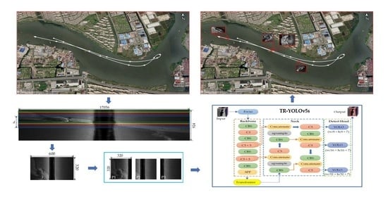
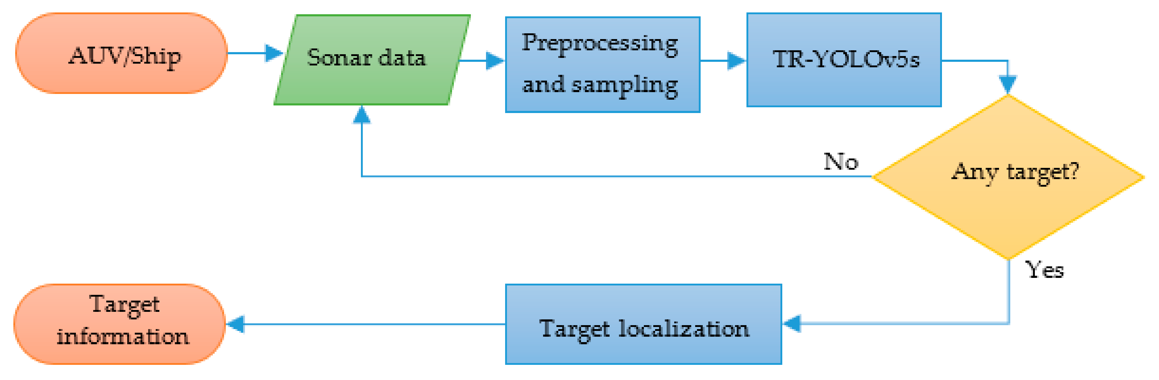
- A real-time SSS ATR method is proposed, including preprocessing, sampling, target recognition by TR–YOLOv5s and target localization;
- To deal with the target-sparse and feature-barren characteristics of SSS image, the attention mechanism is introduced by improving the state-of-the-art (SOTA) object detection algorithm YOLOv5s with transformer module;
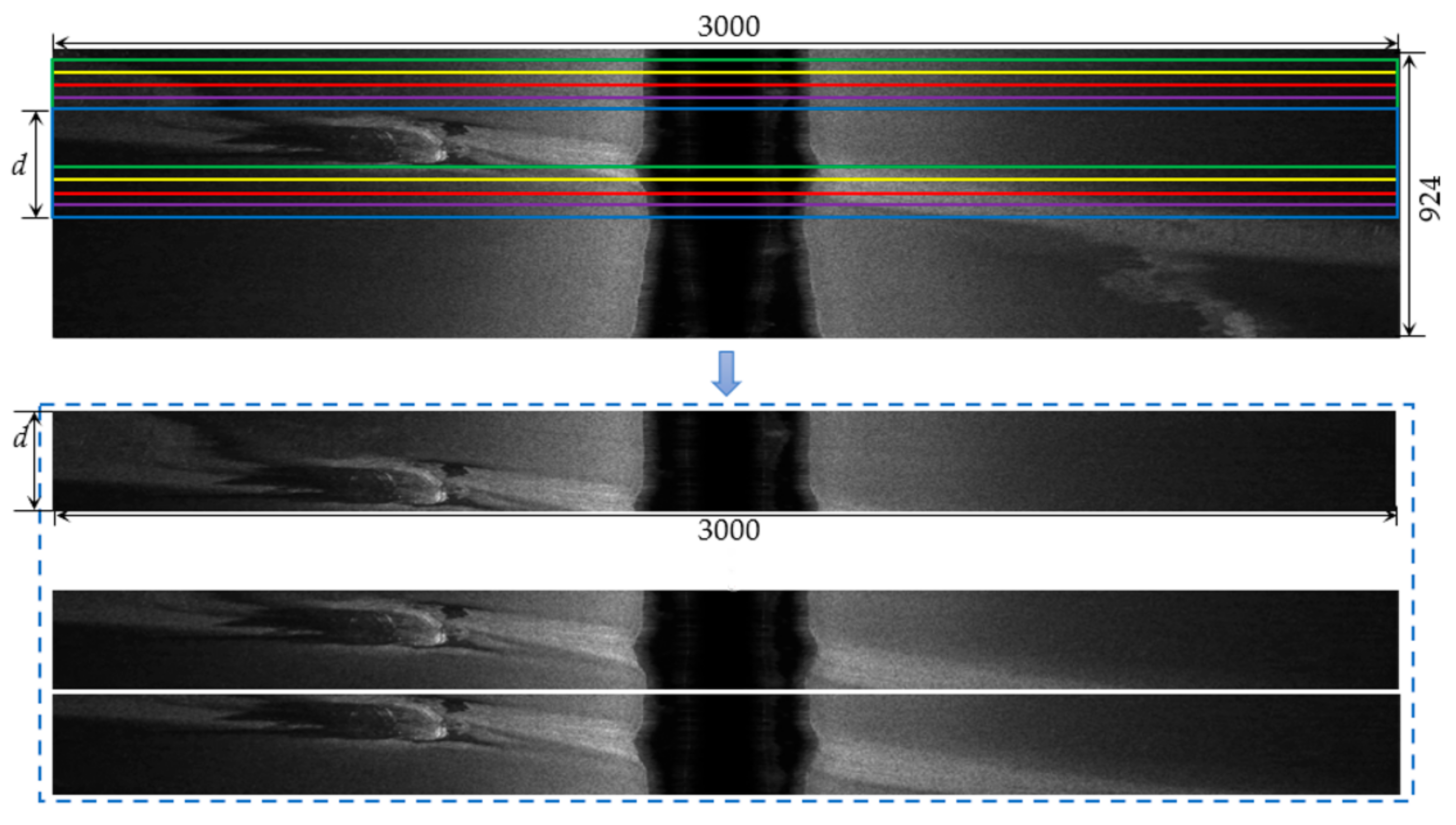
- A down-sampling principle is proposed for the echoes of cross-track direction to maintain the actual aspect ratio of target roughly and reduce the amount of calculation for real-time recognition.
2. Materials and Methods
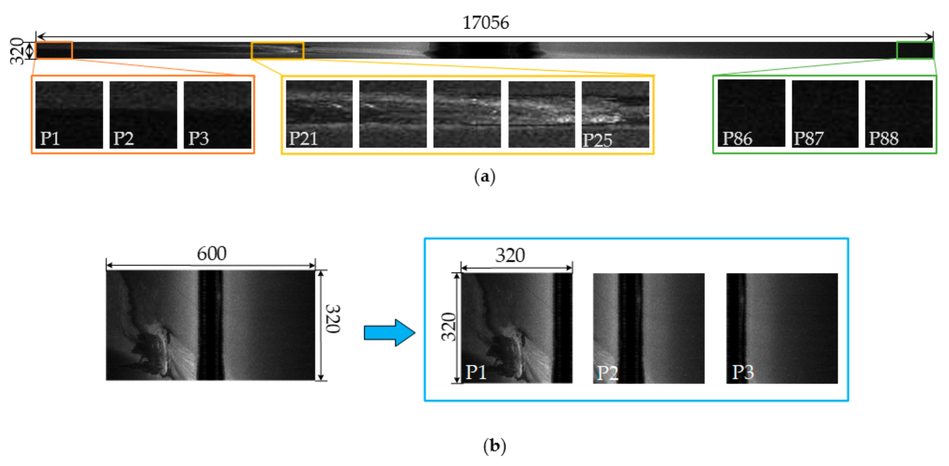
2.1. SSS Image Preprocessing and Sampling
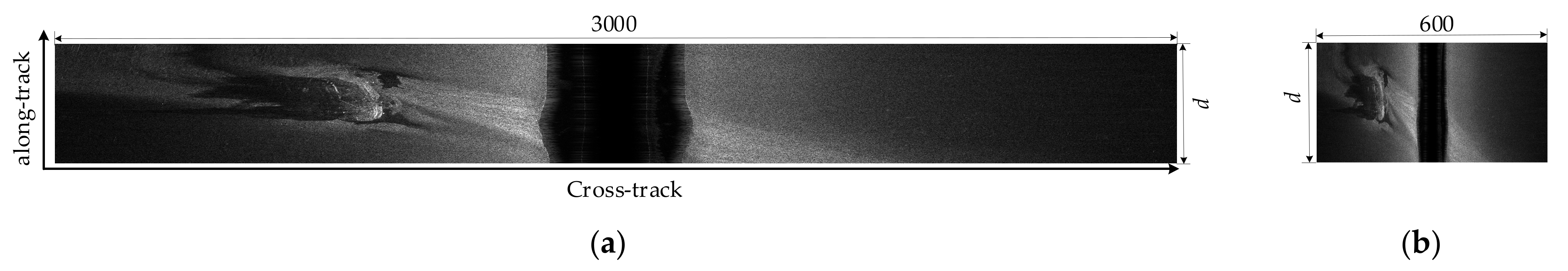
2.1.1. Image Preprocessing
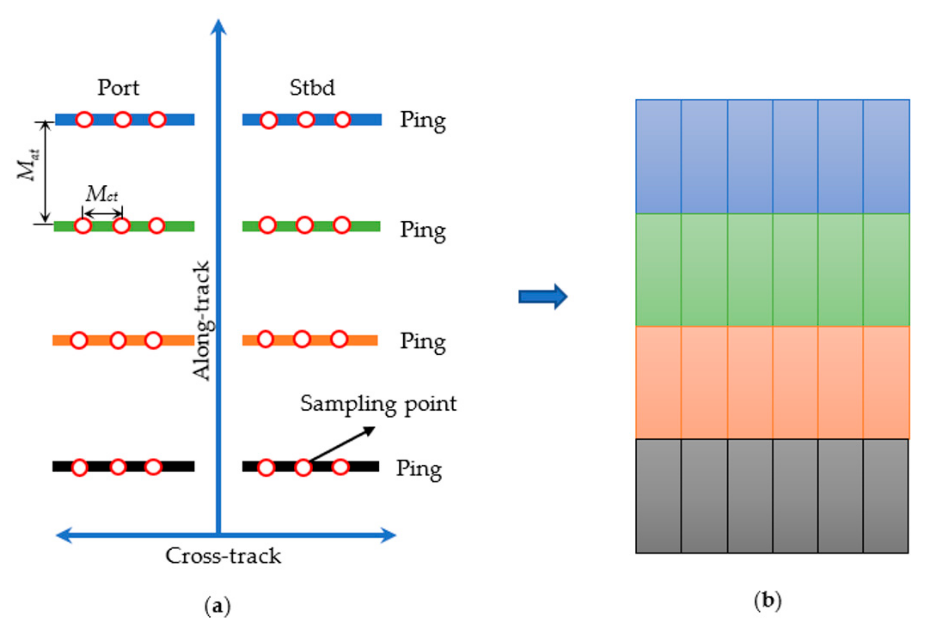
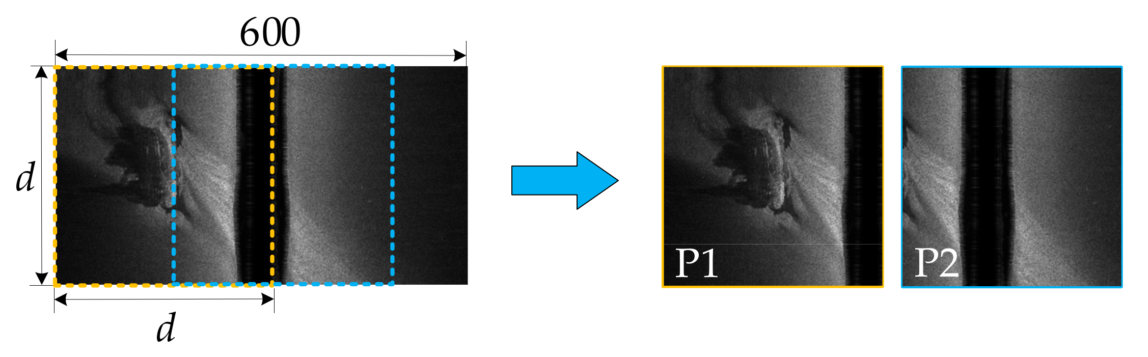
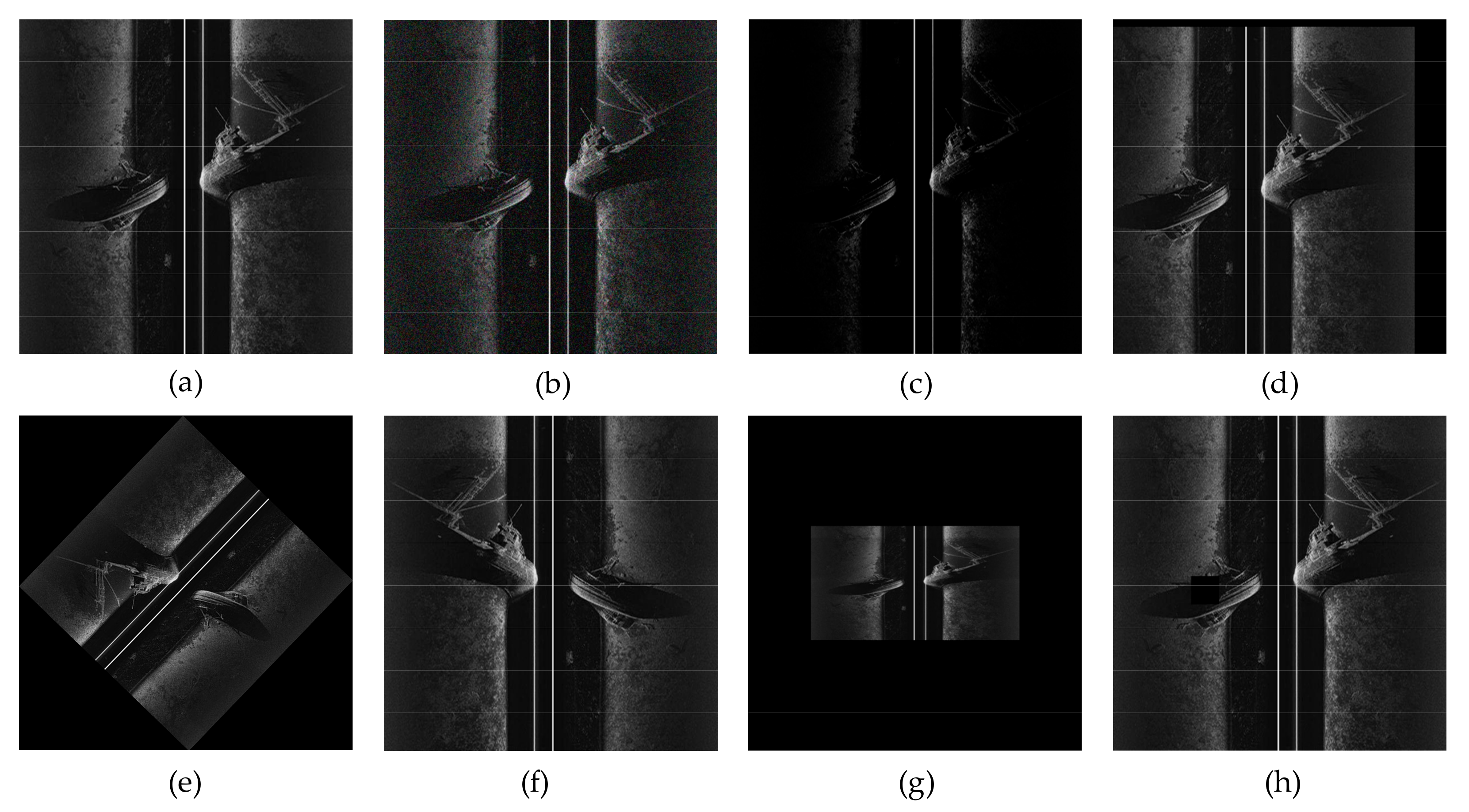
2.1.2. SSS Image Sampling
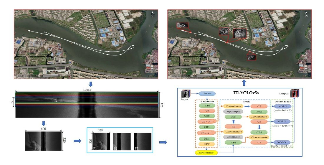
2.2. TR–YOLOv5s
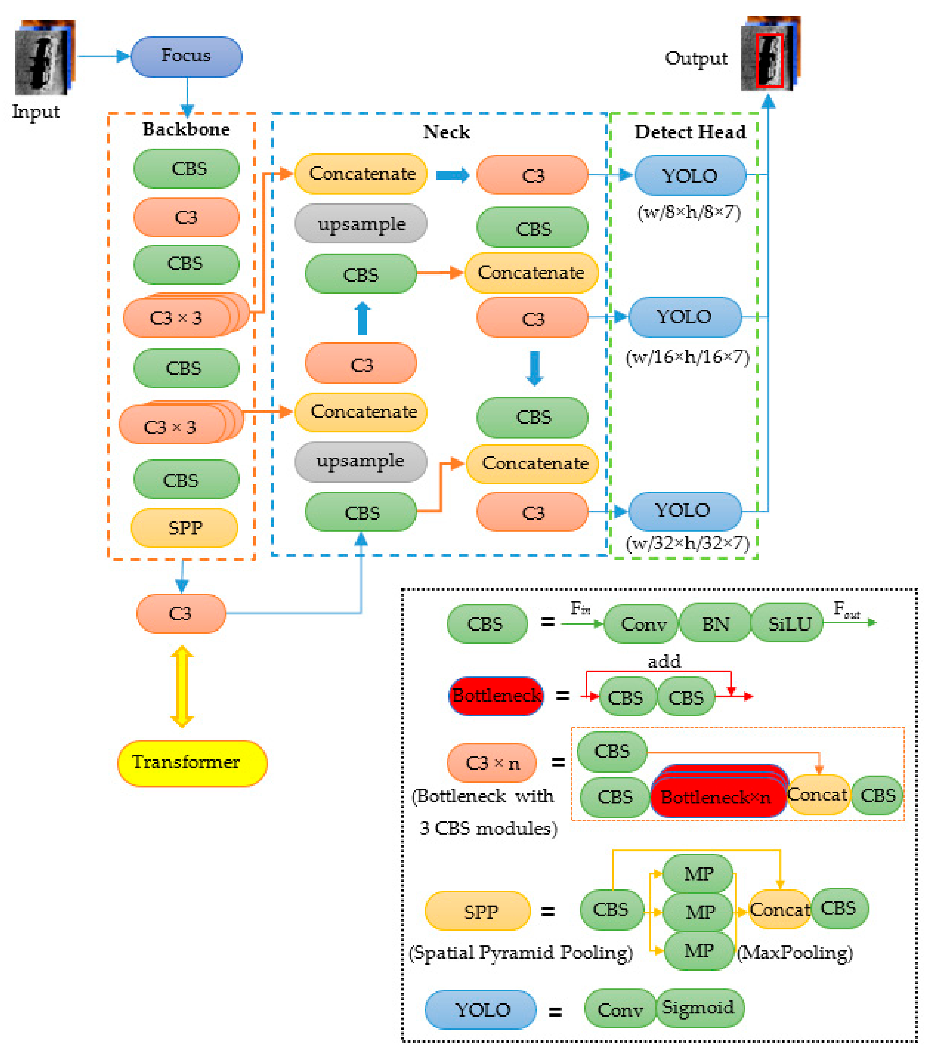
2.2.1. Architecture of TR–YOLOv5s
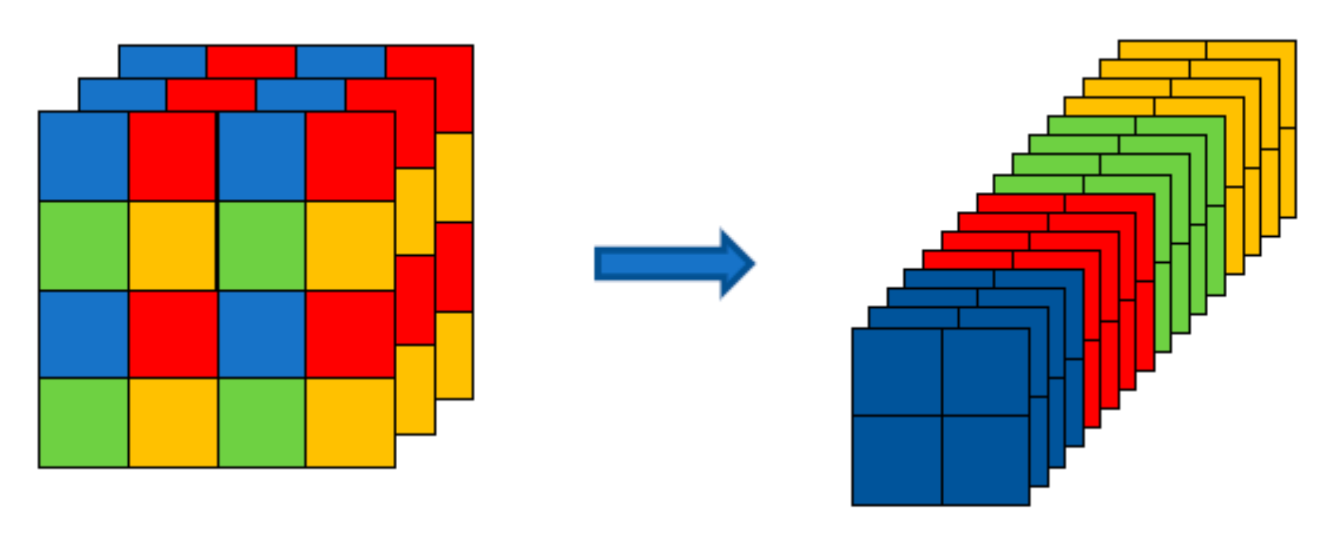
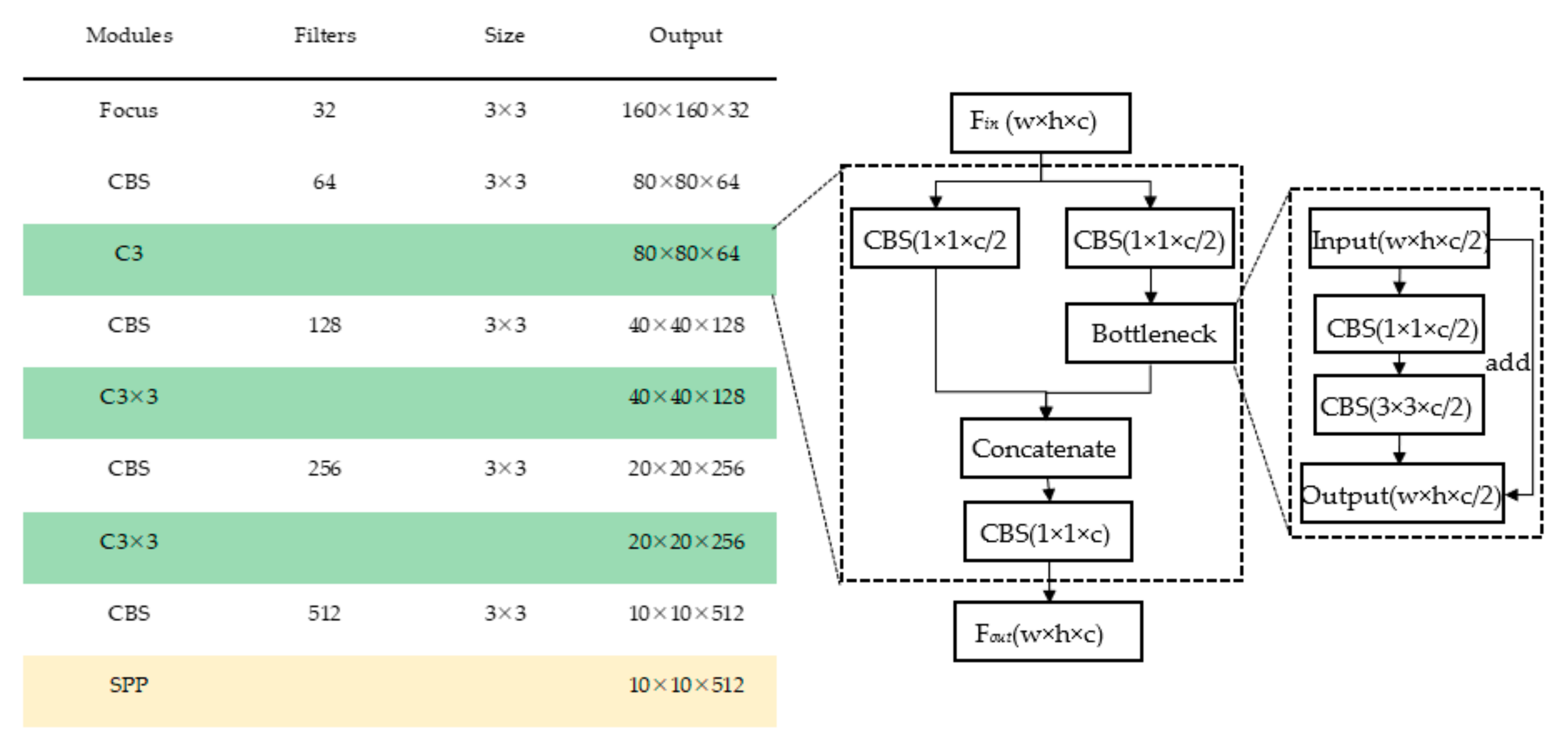
- Backbone
- Neck
- The Detect Head
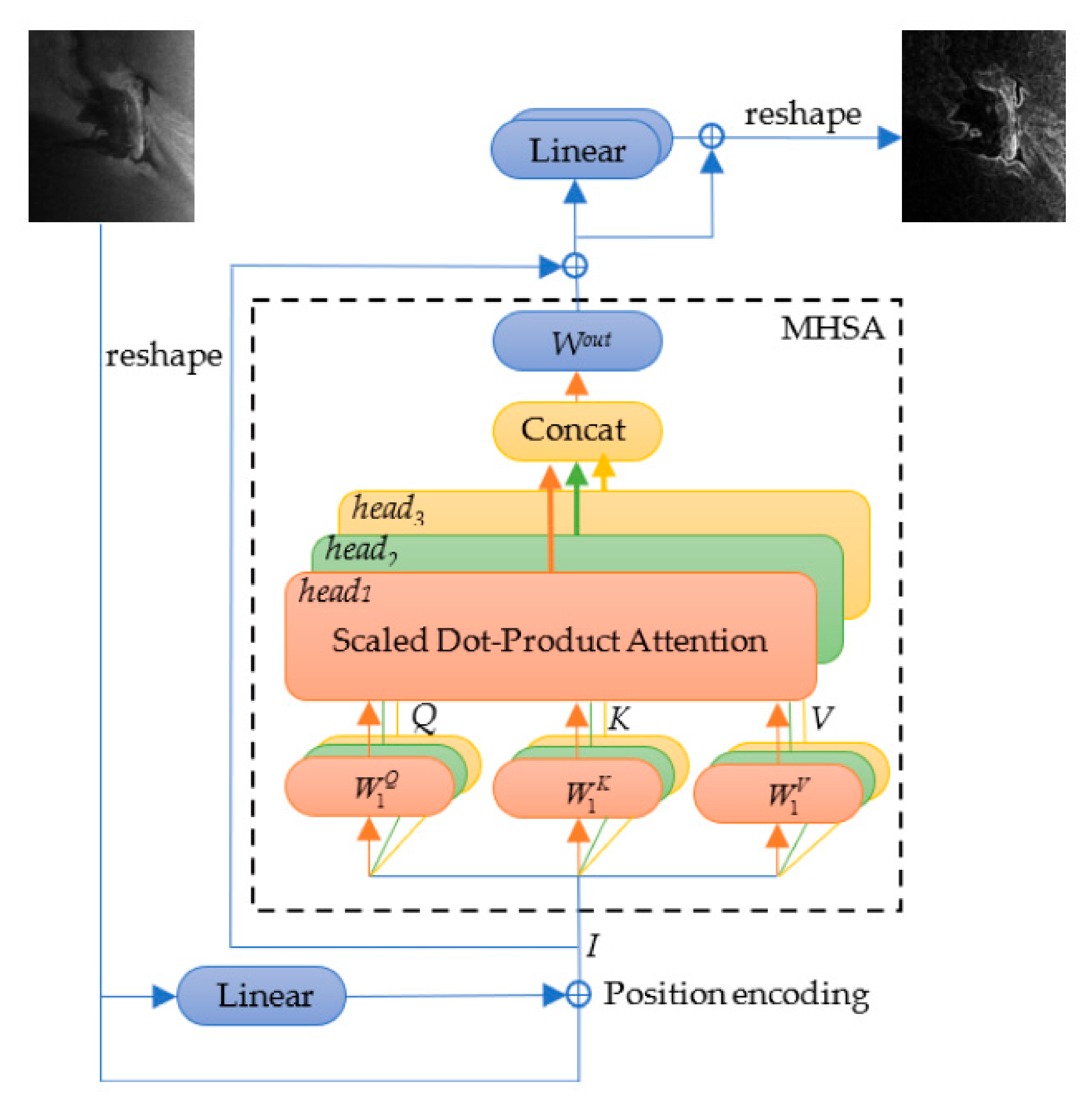
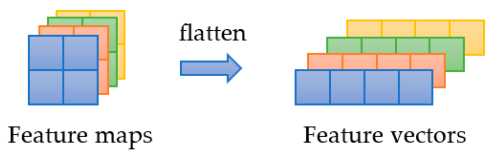
2.2.2. Transformer Module
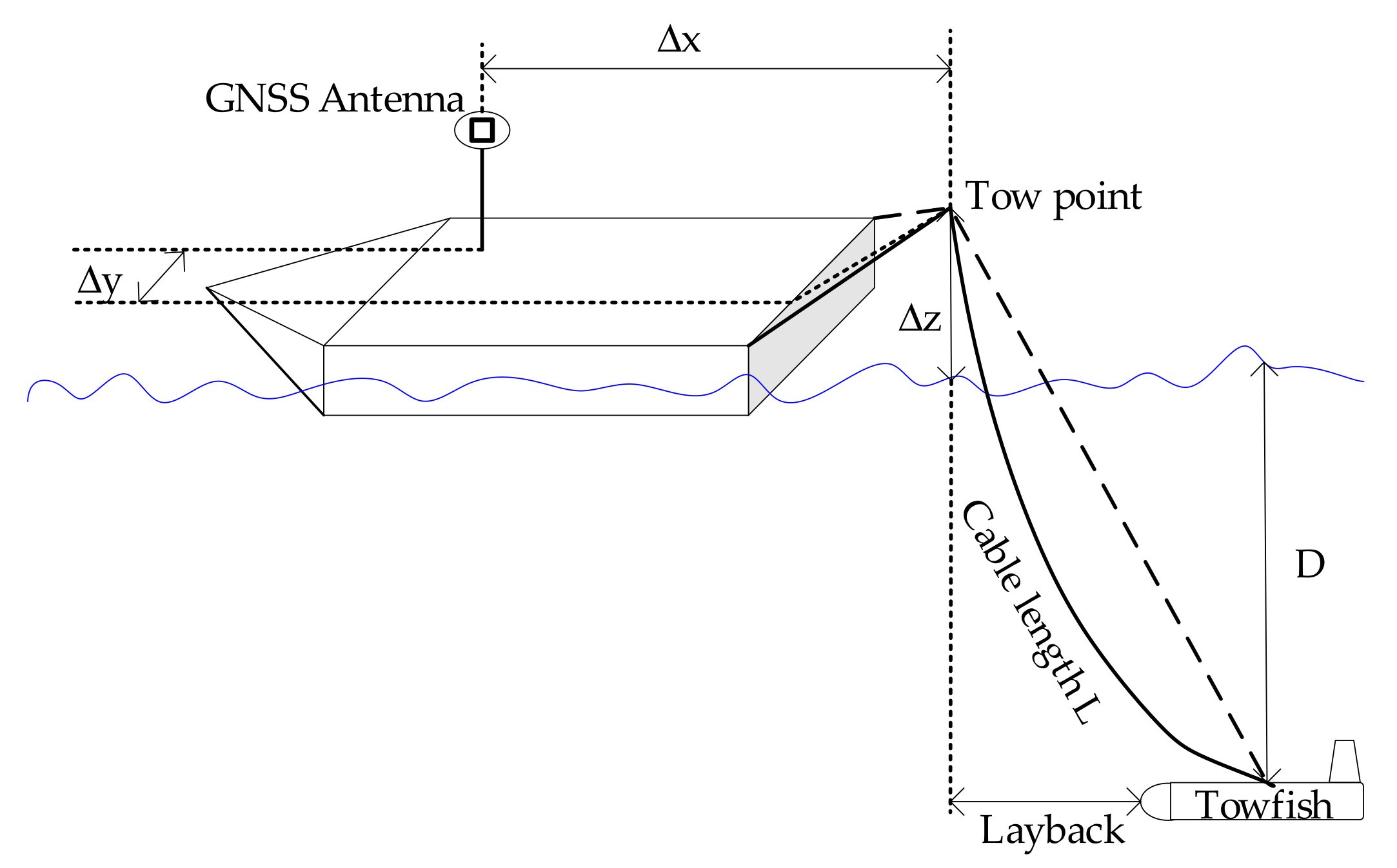
2.3. Target Localization
2.4. Evalution of the Recognition Model
3. Results
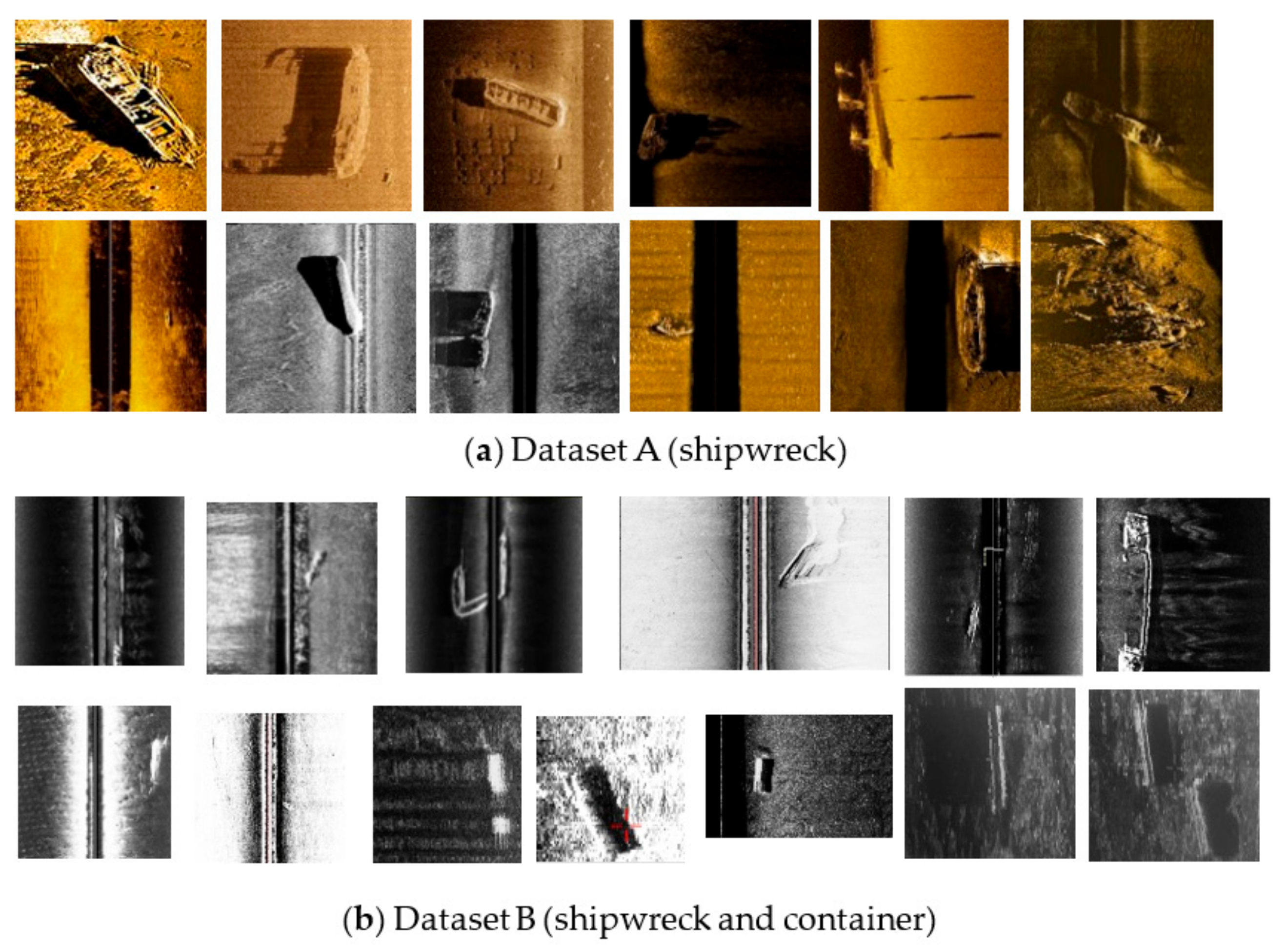
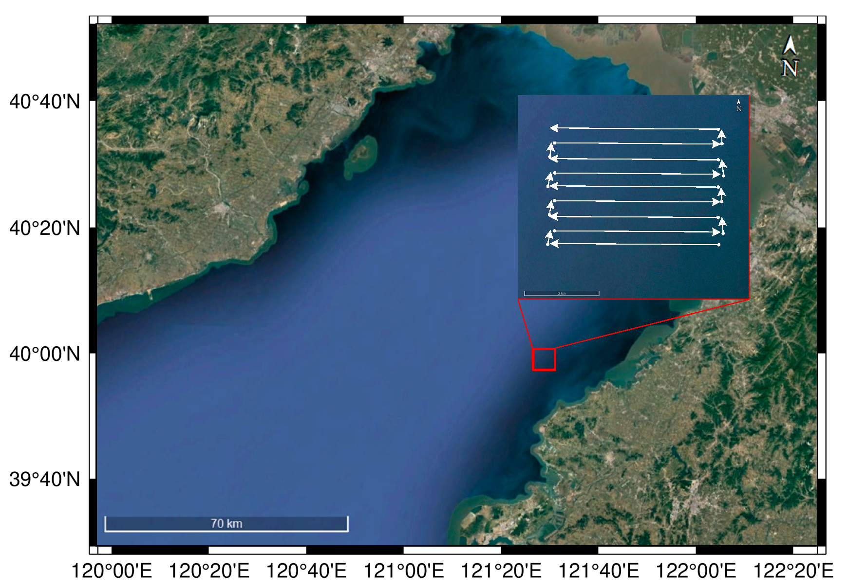
3.1. Dataset
3.1.1. SSS Image Set for Detector Building
3.1.2. Description of Shipwreck Data
3.1.3. Description of Submarine Container Data
3.2. Detector Building
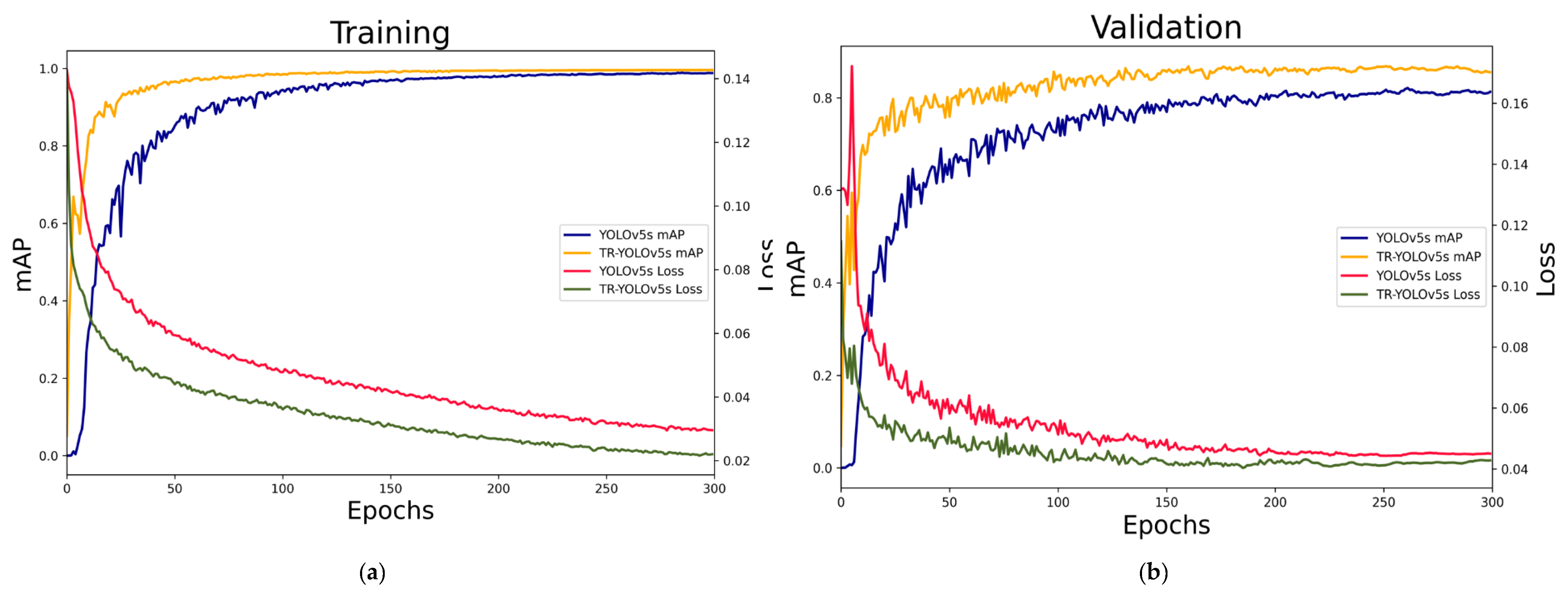
3.2.1. Detector Training
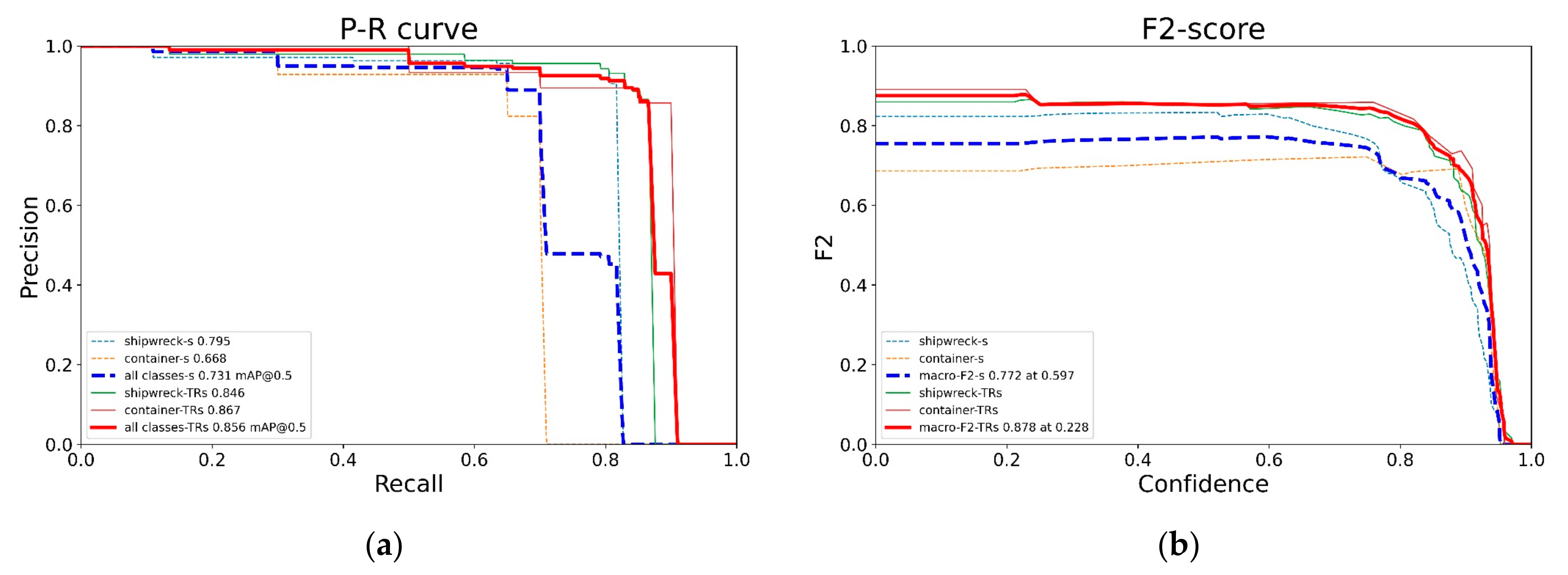
3.2.2. Detector Evaluation
- Pre-trained TR–YOLOv5s achieved a better performance in detection quality and model complexity than YOLOv5s.
- The AUC of pre-trained TR–YOLOv5s, which is equal to the mAP value, is more than that of YOLOv5s. The same conclusion can also be drawn according to the AP values. The macro-F2 curves and the curves of each class target achieved by pre-trained TR–YOLOv5s are above the curves achieved by YOLOv5s. Pre-trained TR–YOLOv5s has better precision and recall than YOLOv5s at almost all the IOU thresholds.
3.2.3. Ablation Study
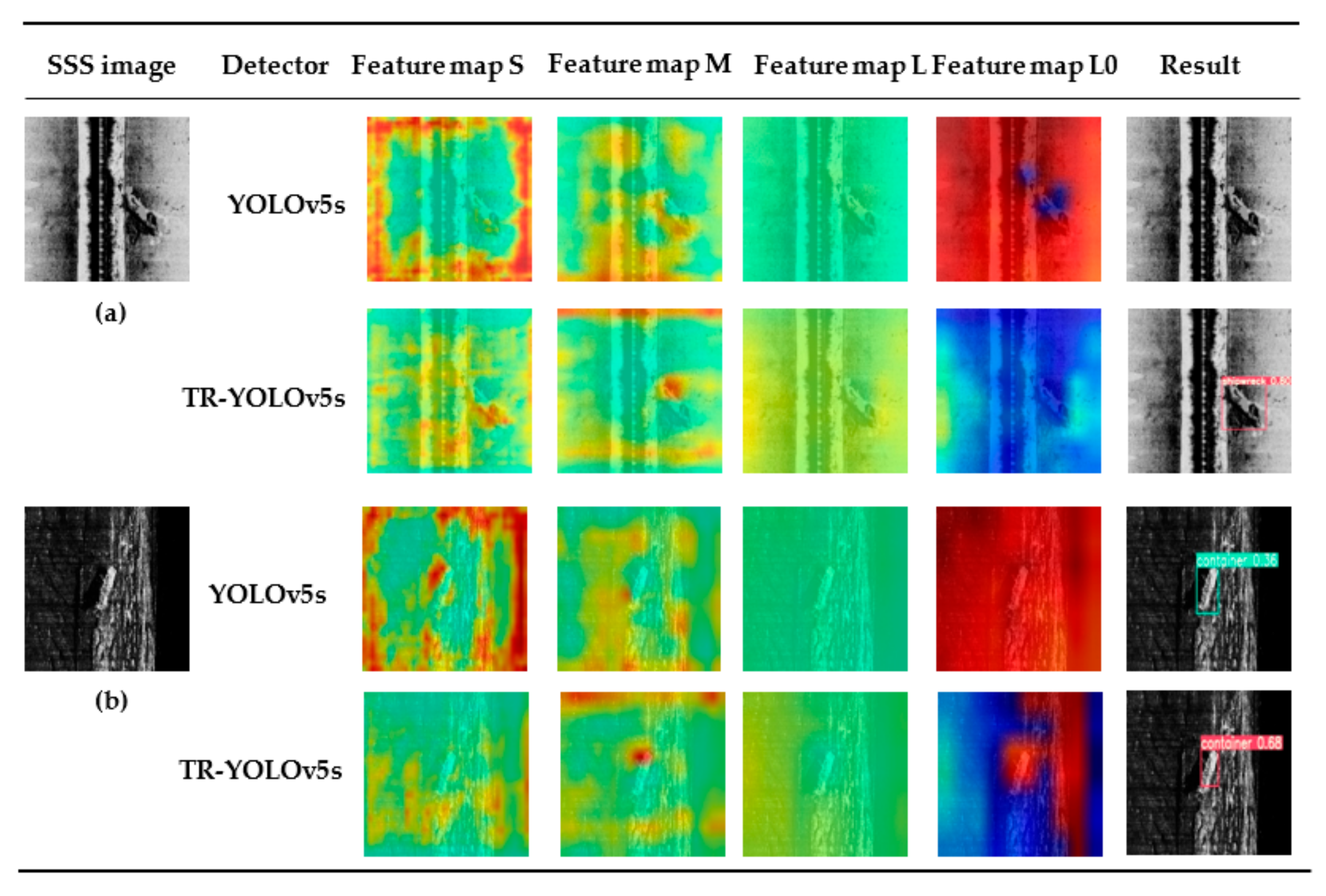
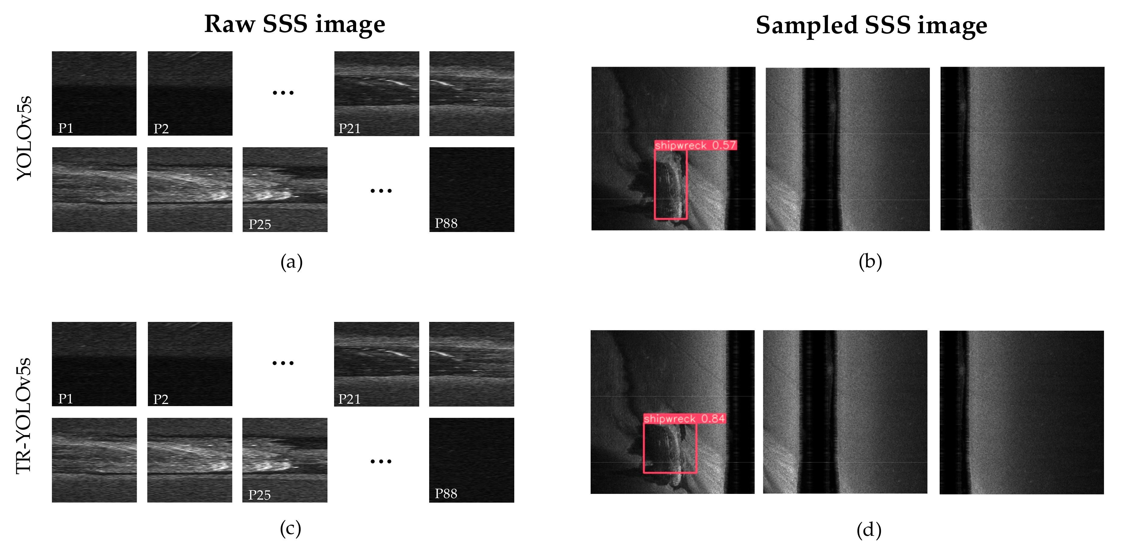
3.2.4. Qualitative Results and Analysis
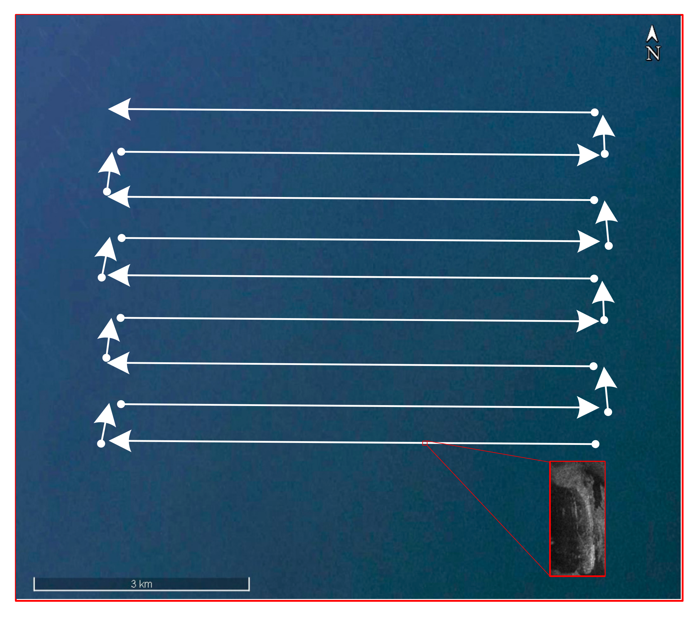
3.3. Single Shipwreck ATR
3.3.1. SSS Image Preprocessing and Sampling
3.3.2. Performance of the Detectors
3.3.3. Target Localization
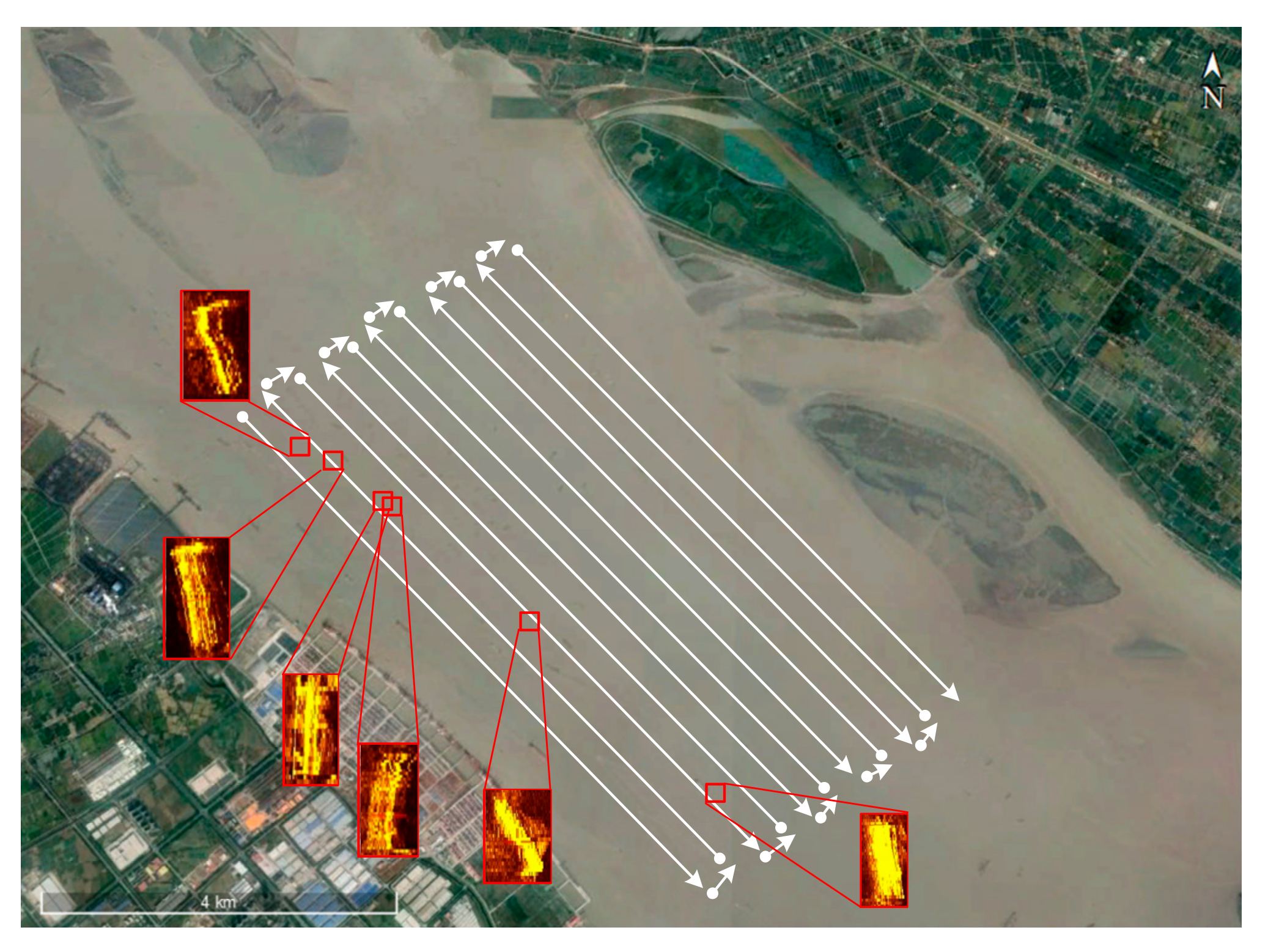
3.4. Multi-Target ATR
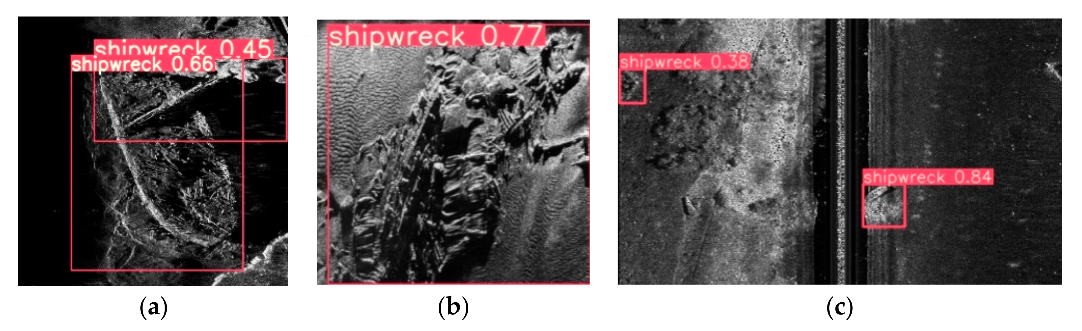
3.4.1. Multi-Shipwreck ATR
3.4.2. Multi-Container ATR
4. Discussion
4.1. Significance of the Proposed Method
4.2. Sensitivity Analysis
4.2.1. The Heads Number in the Transformer Module
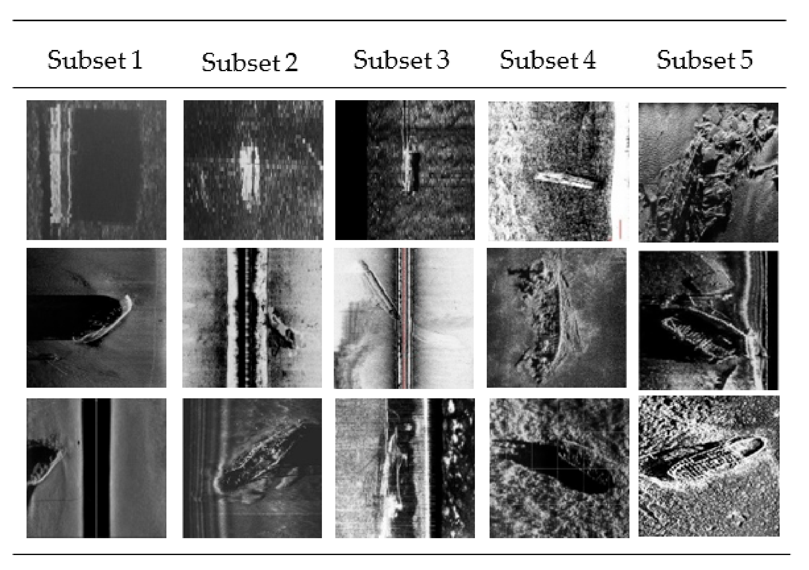
4.2.2. The Complexity of the SSS Images
4.2.3. The Measurement Conditions
4.3. Performance of Detector in Unbenign Seabed
4.4. Comparison with Existing Methods
4.5. Limitations of the Proposed Method
5. Conclusions and Recommendations
Author Contributions
Funding
Data Availability Statement
Acknowledgments
Conflicts of Interest
References
- Celik, T.; Tjahjadi, T. A Novel Method for Sidescan Sonar Image Segmentation. IEEE J. Ocean. Eng. 2011, 36, 186–194. [Google Scholar] [CrossRef]
- Zheng, G.; Zhang, H.; Li, Y.; Zhao, J. A Universal Automatic Bottom Tracking Method of Side Scan Sonar Data Based on Semantic Segmentation. Remote Sens. 2021, 13, 1945. [Google Scholar] [CrossRef]
- Li, S.; Zhao, J.; Zhang, H.; Bi, Z.; Qu, S. A Novel Horizon Picking Method on Sub-Bottom Profiler Sonar Images. Remote Sens. 2020, 12, 3322. [Google Scholar] [CrossRef]
- Barngrovver, C.; Althoff, A.; DeGuzman, P.; Kastner, R. A brain computer interface (BCI) for the detection of mine-like objects in sidescan sonar imagery. IEEE J. Ocean. Eng. 2016, 41, 123–138. [Google Scholar] [CrossRef] [Green Version]
- Lehardy, P.K.; Moore, C. Deep ocean search for Malaysia airlines flight 370. In 2014 Oceans—St. Jhons’s, St. John’s; IEEE: Piscataway, NJ, USA, 2014; pp. 1–4. [Google Scholar]
- Neupane, D.; Seok, J. A Review on Deep Learning-Based Approaches for Automatic Sonar Target Recognition. Elecronics 2020, 9, 1972. [Google Scholar] [CrossRef]
- Zheng, L.; Tian, K. Detection of Small Objects in Sidescan Sonar Images Based on POHMT and Tsallis Entropy. Signal. Process. 2017, 142, 168–177. [Google Scholar] [CrossRef]
- Fakiris, E.; Papatheodorou, G.; Geraga, M.; Ferentinos, G. An Automatic Target Detection Algorithm for Swath Sonar Backscatter Imagery, Using Image Texture and Independent Component Analysis. Remote Sens. 2016, 8, 373. [Google Scholar] [CrossRef] [Green Version]
- Xiao, W.; Zhao, J.; Zhu, B.; Jiang, T.; Qin, T. A Side Scan Sonar Image Target Detection Algorithm Based on a Neutrosophic Set and Diffusion Maps. Remote Sens. 2018, 10, 295. [Google Scholar] [CrossRef] [Green Version]
- Guillaume, L.; Sylvain, G. Unsupervised extraction of underwater regions of interest in sidescan sonar imagery. J. Ocean. Eng. 2020, 15, 95–108. [Google Scholar]
- Zhu, B.; Wang, X.; Chu, Z.; Yang, Y.; Shi, J. Active Learning for Recognition of Shipwreck Target in Side-Scan Sonar Image. Remote Sens. 2019, 11, 243. [Google Scholar] [CrossRef] [Green Version]
- Nargesian, F.; Samulowitz, H.; Khurana, U.; Khalil, E.B.; Turaga, D. Learning Feature Engineering for Classification. In Proceedings of the 26th International Joint Conference on Artificial Intelligence, Melbourne, Australia, 19–25 August 2017; pp. 2529–2535. [Google Scholar]
- Nguyen, H.; Lee, E.; Lee, S. Study on the Classification Performance of Underwater Sonar Image Classification Based on Convolutional Neural Networks for Detecting a Submerged Human Body. Sensors 2019, 20, 94. [Google Scholar] [CrossRef] [Green Version]
- Bore, N.; Folkesson, J. Modeling and Simulation of Sidescan Using Conditional Generative Adversarial Network. IEEE J. Ocean. Eng. 2020, 46, 195–205. [Google Scholar] [CrossRef]
- Steiniger, Y.; Kraus, D.; Meisen, T. Generating Synthetic Sidescan Sonar Snippets Using Transfer-Learning in Generative Adversarial Networks. J. Mar. Sci. Eng. 2021, 9, 239. [Google Scholar] [CrossRef]
- Lee, S.; Park, B.; Kim, A. Deep Learning based Object Detection via Style-transferred Underwater Sonar Images. In Proceedings of the 12th IFAC Conference on Control Applications in Marine Systems, Robotics, and Vehicles CAMS 2019, Daejeon, Korea, 18–20 September 2019; pp. 152–155. [Google Scholar]
- Kim, J.; Choi, J.; Kwon, H.; Oh, R.; Son, S. The application of convolutional neural networks for automatic detection of underwater object in side scan sonar images. J. Acoust. Soc. Korea 2018, 37, 118–128. [Google Scholar]
- Einsidler, D.; Dhanak, M.; Beaujean, P. A Deep Learning Approach to Target Recognition in Side-Scan Sonar Imagery. In Proceedings of the MTS/IEEE Charleston OCEANS Conference, Charleston, SC, USA, 22–25 October 2018; pp. 1–4. [Google Scholar]
- Nayak, N.; Nara, M.; Gambin, T.; Wood, Z.; Clark, C.M. Machine learning techniques for AUV side scan sonar data feature extraction as applied to intelligent search for underwater archaeology sites. Field Serv. Robot. 2021, 16, 219–233. [Google Scholar]
- Huo, G.; Wu, Z.; Li, J. Underwater Object Classification in Sidescan Sonar Images Using Deep Transfer Learning and Semisynthetic Training Data. IEEE Access 2020, 8, 47407–47418. [Google Scholar] [CrossRef]
- Li, C.L.; Ye, X.F.; Cao, D.X.; Hou, J.; Yang, H.B. Zero shot objects classification method of side scan sonar image based on synthesis of pseudo samples. Appl. Acoust. 2021, 173, 107691. [Google Scholar] [CrossRef]
- Song, Y.; He, B.; Liu, P. Real-Time Object Detection for AUVs Using Self-Cascaded Convolutional Neural Networks. IEEE J. Ocean. Eng. 2019, 46, 56–67. [Google Scholar] [CrossRef]
- Wu, M.; Wang, Q.; Rigall, E.; Li, K.; Zhu, W.; He, B.; Yan, T. ECNet: Efficient Convolutional Networks for Side Scan Sonar Image Segmentation. Sensors 2019, 19, 2009. [Google Scholar] [CrossRef] [Green Version]
- Burguera, A.; Bonin-Font, F. On-Line Multi-Class Segmentation of Side-Scan Sonar Imagery Using an Autonomous Underwater Vehicle. J. Mar. Sci. Eng. 2020, 8, 557. [Google Scholar] [CrossRef]
- Ultralytics-Yolov5. Available online: https://github.com/ultralytics/yolov5 (accessed on 1 January 2021).
- Xu, R.; Lin, H.; Lu, K.; Cao, L.; Liu, Y. A Forest Fire Detection System Based on Ensemble Learning. Forests 2021, 12, 217. [Google Scholar] [CrossRef]
- Loffe, S.; Szegedy, C. Batch normalization: Accelerating deep network training by reducing internal covariate shift. In Proceedings of the 32nd International Conference on International Conference on Machine Learning (ICML), Lile, France, 6–11 July 2015; pp. 448–456. [Google Scholar]
- Elfwing, S.; Uchibe, E.; Doya, K. Sigmoid-weighted linear units for neural network function approximation in reinforcement learning. Neural Netw. 2018, 107, 3–11. [Google Scholar] [CrossRef] [PubMed]
- Wang, C.; Liao, H.M.; Wu, Y.; Chen, P.; Hsieh, J.; Yeh, I. CSPNet: A New Backbone that can Enhance Learning Capability of CNN. In Proceedings of the 2020 IEEE/CVF Conference on Computer Vision and Pattern Recognition Workshops (CVPRW), Seattle, WA, USA, 14–19 June 2020; pp. 1571–1580. [Google Scholar]
- Lin, T.; Dollár, P.; Girshick, R.; He, K.; Hariharan, B.; Belongie, S. Feature Pyramid Networks for Object Detection. In Proceedings of the 2017 IEEE Conference on Computer Vision and Pattern Recognition (CVPR), Honolulu, HI, USA, 21–26 July 2017; pp. 936–944. [Google Scholar]
- Liu, S.; Qi, L.; Qin, H.; Shi, J.; Jia, J. Path Aggregation Network for Instance Segmentation. In Proceedings of the 2018 IEEE/CVF Conference on Computer Vision and Pattern Recognition, Salt Lake City, UT, USA, 18–23 June 2018; pp. 8759–8768. [Google Scholar]
- Redmon, J.; Farhadi, A. YOLOv3: An incremental improvement. arXiv 2018, arXiv:1804.02767. [Google Scholar]
- Vaswani, A.; Shazeer, N.; Parmar, N.; Uszkoreit, J.; Jones, L.; Gomez, A.N.; Kaiser, L.; Polosukhin, I. Attention is all you need. In Proceedings of the 31st International Conference on Neural Information Processing Systems (NIPS), Long Beach, CA, USA, 4–9 December 2017; pp. 6000–6010. [Google Scholar]


| Data Set | Training Set | Validation Set | Test Set | |||||||
|---|---|---|---|---|---|---|---|---|---|---|
| Target | A | B | Total | A | B | Total | A | B | Total | |
| Shipwreck | 194 | 34 | 228 | 56 | 20 | 76 | 63 | 11 | 74 | |
| Container | 0 | 58 | 58 | 0 | 19 | 19 | 0 | 20 | 20 | |
| Total | 194 | 92 | 286 | 56 | 39 | 95 | 63 | 31 | 94 | |
| Data Set | Training Set | Validation Set | Test Set | |||||||
|---|---|---|---|---|---|---|---|---|---|---|
| Target | A | B | Total | A | B | Total | A | B | Total | |
| Shipwreck | 970 | 170 | 1140 | 280 | 100 | 380 | 63 | 11 | 74 | |
| Container | 0 | 1160 | 1160 | 0 | 380 | 380 | 0 | 20 | 20 | |
| Total | 970 | 1330 | 2300 | 280 | 480 | 760 | 63 | 31 | 94 | |
| Detector | Target | AP@0.5 1 | mAP@0.5 1 | macro-F2 | GFLOPs 2 |
|---|---|---|---|---|---|
| YOLOv5s | Shipwreck | 79.5% | 73.1% | 77.2%@0.60 3 | 16.3 |
| Container | 66.8% | ||||
| Pre-trained TR–YOLOv5s | Shipwreck | 84.6% | 85.6% | 87.8%@0.23 3 | 16.2 |
| Container | 86.7% |
| Pre-Trained | Transformer | Precision | Recall | mAP@0.5 1 | Macro-F2 | GFLOPs 2 |
|---|---|---|---|---|---|---|
| 87.3% | 74.6% | 73.1% | 77.2%@0.60 3 | 16.3 | ||
| ✓ | 92.2% | 75.3% | 81.6% | 81.5%@0.24 | 16.2 | |
| ✓ | 91.3% | 77.8% | 79.1% | 81.8%@0.31 | 16.3 | |
| ✓ | ✓ | 90.9% | 84% | 85.6% | 87.8%@0.23 | 16.2 |
| Detector | TP | FP | TP + FN | Precision | Recall | Time |
|---|---|---|---|---|---|---|
| YOLOv5s | 250 | 30 | 348 | 89.3% | 71.8% | 0.033 |
| TR–YOLOv5s | 329 | 0 | 348 | 100% | 94.5% | 0.036 |
| Head | 2 | 4 | 8 | 16 | 32 | 64 | |
|---|---|---|---|---|---|---|---|
| Index | |||||||
| mAP@0.5 | 83.3% | 85.6% | 82.2% | 82.2% | 79.9% | 81.8% | |
| Macro-F2 | 84.8% | 87.8% | 84.4% | 85.3% | 82.6% | 83.9% | |
| Subset | 1 | 2 | 3 | 4 | 5 | |
|---|---|---|---|---|---|---|
| Index | ||||||
| Complexity | 0–170 | 170–270 | 270–360 | 360–530 | 530–1600 | |
| Numbers | 20 | 20 | 20 | 20 | 14 | |
| mAP@0.5 | 90.1% | 91.7% | 77.4% | 89.7% | 81.4% | |
| Num | Method | Algorithm | Task | Object | Accuracy | Efficiency |
|---|---|---|---|---|---|---|
| 1 | Our method | TR–YOLOv5s | Detection | Shipwreck Container | 85.6% (mAP, Laboratory) | 0.068 milliseconds per 100 pixels (Ship) |
| 2 | Song et al. (2019) [22] | Self-Cascaded CNN | Segmentation | Highlight Shadow Seafloor | 57.6~97.1% (mIOU 1, Laboratory) | 0.067 s per ping (AUV) |
| 3 | Wu et al. (2019) [23] | Depth-Wise Separable Convolution | Segmentation | Object Background | 66.2% (mIOU, Laboratory) | 0.038 milliseconds per 100 pixels (Laboratory) |
| 4 | Burguera et al. (2020) [24] | Fully convolutional neural network | Segmentation | Rock Sand Other | 87.8% (F1 score, AUV) | 4.6 milliseconds per 100 pixels (AUV) |
Publisher’s Note: MDPI stays neutral with regard to jurisdictional claims in published maps and institutional affiliations. |
© 2021 by the authors. Licensee MDPI, Basel, Switzerland. This article is an open access article distributed under the terms and conditions of the Creative Commons Attribution (CC BY) license (https://creativecommons.org/licenses/by/4.0/).
Share and Cite
Yu, Y.; Zhao, J.; Gong, Q.; Huang, C.; Zheng, G.; Ma, J. Real-Time Underwater Maritime Object Detection in Side-Scan Sonar Images Based on Transformer-YOLOv5. Remote Sens. 2021, 13, 3555. https://doi.org/10.3390/rs13183555
Yu Y, Zhao J, Gong Q, Huang C, Zheng G, Ma J. Real-Time Underwater Maritime Object Detection in Side-Scan Sonar Images Based on Transformer-YOLOv5. Remote Sensing. 2021; 13(18):3555. https://doi.org/10.3390/rs13183555
Chicago/Turabian StyleYu, Yongcan, Jianhu Zhao, Quanhua Gong, Chao Huang, Gen Zheng, and Jinye Ma. 2021. "Real-Time Underwater Maritime Object Detection in Side-Scan Sonar Images Based on Transformer-YOLOv5" Remote Sensing 13, no. 18: 3555. https://doi.org/10.3390/rs13183555