First Estimation of Global Trends in Nocturnal Power Emissions Reveals Acceleration of Light Pollution

Abstract

The global spread of artificial light is eroding the natural night-time environment. The estimation of the pattern and rate of growth of light pollution on multi-decadal scales has nonetheless proven challenging. Here we show that the power of global satellite observable light emissions increased from 1992 to 2017 by at least 49%. We estimate the hidden impact of the transition to solid-state light-emitting diode (LED) technology, which increases emissions at visible wavelengths undetectable to existing satellite sensors, suggesting that the true increase in radiance in the visible spectrum may be as high as globally 270% and 400% on specific regions. These dynamics vary by region, but there is limited evidence that advances in lighting technology have led to decreased emissions.

1. Introduction

Satellite images of the Earth at night strikingly illustrate the extent of the distribution of artificial light sources associated with human settlement, industry and transport links, across its surface [1]. The quantity of artificial light detected from satellites includes a mixed signal of direct emissions from outdoor lighting that is not vertically shielded, as well as reflected light from the ground, buildings and vegetation, and light scattered within the atmosphere. This signal has increasingly been used as an important indicator of urbanisation, industrial activity [2,3] and economic development [4,5]. It has also been used as a measure of light pollution [6,7], which has long been a concern of astronomers [8,9] but has more recently been proposed as an emerging major threat both to public health and natural ecosystems. Indeed, light pollution has been implicated in increased human cancer risk [10,11], population declines in wild species [12,13], the restructuring of ecological communities [14,15], and the disruption of key ecosystem services such as pollination [16,17].

To determine how the global magnitude of the impacts of light pollution is changing on multi-decadal scales, as has been performed for many other anthropogenic environmental pressures, time series data on artificial light emissions are required. This proved challenging for a combination of reasons, including technical difficulties in distinguishing faint artificial light sources from natural ones, limitations of the available satellite sensors, and a paucity of ground-truthed sources. In consequence, studies to date [18,19] have been severely limited in their spatial and temporal coverage, and in the inferences that could be drawn. Here we provide a global estimation of changes in artificial night-time lighting over a 25-year period, using ground-truth data and a conservative estimation of the potential errors associated particularly with a lack of information on emissions in the blue part of the spectrum.

The Defense Meteorological Satellite Program Operational Line scan System (DMSP-OLS) forms the basis for the longest publicly available time series of artificial light at night from space, with uncalibrated composite images freely obtainable from a digital archive since 1992 [20]. Since December 2011, the Visible Infrared Imaging Radiation Suite (VIIRS) Day/Night Band (DNB) on board the NASA/NOAA Suomi National Polar-orbiting Partnership (Suomi-NPP) satellite has provided a radiance calibrated product with global coverage. However, quantifying changes in artificial light emissions at night at the global scale from satellite imagery was hindered by several factors.

First, the lack of on-board calibration of the DMSP-OLS images means that irradiance values from different images from the satellite cannot be directly compared without complex cross-calibration. The sensor performance degrades with time and varies between images, years and satellites, calibrations are adjusted “on the fly” and, due to the low memory range and low dynamic range of the sensor, archived radiance values are represented in images as an uncalibrated digital number (DN) between 1 and 63, which cannot be compared between different composite images in a straightforward manner.

Second, in brightly lit urban and industrial areas the signal in DMSP-OLS data frequently reaches saturation at a DN of 63, making change detection within such areas impossible [21].

Third, the resolution of DMSP-OLS images is fairly low (2.7 km), the accuracy of georeferencing is often poor and images suffer from “blooming” effects [22], resulting in a blurred image around bright light sources, making the identification of fine scale features problematic [23].

Fourth, the single-channel spectral response of the DMSP-OLS sensor is close to zero at wavelengths of visible light below 500 nm. White phosphor-based LED lighting typically emits at a peak radiance of around 465 nm, and so as outdoor lighting increasingly switches from gas-discharge technologies such as high-pressure sodium to solid-state LED lighting, an undetermined, but increasing, proportion of emitted light is undetected (Figure 1). This is particularly significant, because LED lighting has been widely championed as a technological revolution with increased energy efficiency compared with other white light sources, that enables the potential of outdoor lighting at reduced carbon dioxide emissions and financial costs, but recent analysis suggests that these reduced costs may encourage increased overall light emissions [19].

Some, but not all, of the issues associated with tracking global artificial night-time light emissions were resolved with the availability of the VIIRS-DNB imagery from 2012 onwards. VIIRS is radiance calibrated and has a higher dynamic range without saturation, allowing comparison between images and detection of change even within brightly lit areas [23]. It has a higher spatial resolution (740 m), and the archived cloud-free composite products suffer less from errors in georeferencing and “blooming” effects. However, the spectral response of the sensor is similarly low below wavelengths of 500 nm (Figure 1), leaving a proportion of light emitted from LEDs undetected. Recently, images taken from the International Space Station (ISS) [24] and satellites such as JL-13B [25] have provided higher resolution night-time imagery with three-band spectral resolution (red, green, and blue visual bands), potentially allowing changes in lighting technology to be detected directly [24]. However, at present the DMSP-OLS data remain the only source for assessing decadal-scale changes in radiance.

To overcome some of the limitations, methods have been proposed for inter-calibrating archived DMSP-OLS imagery for change detection [2,26,27], and the data set in uncalibrated and cross-calibrated forms has been used widely to investigate economic development and ecological impacts. Since 2016, attempts have been made to provide calibrated ground truthing for night-time light measurements [28]. A radiance calibrated version of the DMSP-OLS data, which does not suffer from saturation effects, was developed [29] in which data are collected at three different fixed gain levels, with a preflight sensor calibration, at the new moon. This method has been used to produce radiance calibrated composite images for the years 1996, 1999, 2000, 2002, 2004, 2005 and 2010.

Here, we produced a global time series of satellite-detectable emitted power of outdoor lighting between 500 nm and 900 nm from 1992 to 2017 by integrating the uncalibrated and radiance-calibrated DMSP-OLS time series, VIIRS imagery and a data set of regional energy consumption by municipal street lighting [30], which is globally the principal source of outdoor artificial light at night. Uncalibrated DMSP-OLS data were fitted to calibrated DMSP-OLS data sets using non-linear regression methods, then all three satellite data sets were calibrated using linear methods to fit to the energy consumption data. Using assumptions about the rate of conversion to solid-state LED lighting, we then estimated the potential range of this “hidden” component of global light at night.

2. Materials and Methods

2.1. Background

To produce a consistent time series of radiance for each country in the world, we undertook four steps in data processing. First, we used a robust regression approach to calibrate the uncalibrated DMSP-OLS images to the nearest calibrated image in time. Second, we assimilated provincial data on energy consumption from street lighting (as a proxy for expected light emissions) to smooth and refine the calibration of all images to produce a consistent time series. Third, we utilised the time difference in image acquisition between the DMSP-OLS and VIIRS satellite images to adjust this time series to produce two separate time series of radiance for each nation state, for early evening and midnight respectively. Fourth, we estimated the effect that changes in light technology towards blue-rich solid-state (LED) lighting may had on detected light emissions since 2012, given the poor detection of blue light by the satellites, and produce high and low estimates of the actual radiance given the detected radiance under three different scenarios of technological change. A summary of the procedure is shown in Figure S1.

2.2. Calibration of Uncalibrated DMSP-OLS Data

The annual, uncalibrated DMSP-OLS data have no absolute or relative intercalibration, and the response of each image to absolute radiance is non-linear. Previous studies have attempted to intercalibrate these images by assuming that certain regions, such as Sicily [31], are essentially invariant in radiance over time and have used conventional regression techniques to intercalibrate global images using such “invariant regions” [32]. However, it is likely that few locations have truly stable lights over several years [33], for example, the island of Sicily increased its energy consumption by street lighting by 20% over 20 years [30]. Lamp “lumen depreciation,” a decay in brightness over time in most bulb technologies as bulbs age, may also limit the effectiveness of intercalibrations, even if the number of light sources and their bulb type remains constant. Other approaches used “robust” regression techniques, such as quantile regression through the median [26] or ridgeline regression [34], which do not assume that entire regions are invariant, but rather that changes within the calibration region are incremental and localised. Such “robust regression” approaches are less sensitive to localised changes than least-squared regression but assume that the brightness of most pixels remains approximately constant between two images, even if localised pixels increase or decrease substantially. More recently, the TERRA-VEGA project [28] attempted to ground-truth artificial light using a mobile source. However, such ground -based calibration sources have only been available since 2016. Recently, calibration of the VIIRS data using stars was performed, but as far as we know not yet implemented for the monthly data composites [35].

In order to calibrate the uncalibrated DMSP-OLS data to radiance values, we used a robust regression method on a calibration area encompassing Italy (bounded between 4 and 19° E and 35.5 and 47° N). We made no assumption that this area has remained unchanged in radiance over time, but rather that most changes in anthropogenic light are incremental and localised in space. This region was selected as it has historical data of energy use in municipal street lighting at the provincial level for use in subsequent calibration steps. We first matched each uncalibrated image with the closest (in time) radiance-calibrated image. Calibrated images exist for 1996, 1999, 2000, 2002, 2004, 2005, 2010 and 2011. Each value in the uncalibrated DMSP images is a digital number (DN) between 0 and 63, while the radiance-calibrated VIIRS and DMSP images are calibrated to nW cm⁻² sr⁻¹ [2]. For each digital number (DN) value of the uncalibrated data within the calibration region, we fitted a kernel density estimation using the density function in the statistical software, R [36]. We then took the maximum value of the kernel density (the mode of the fitted distribution) as the most likely absolute radiance value represented by each digital number. This step was based on the assumption that, while many absolute radiance values may have changed between the acquisition of each uncalibrated image and the nearest calibrated image, the modal value is robust to changes in the extremes of the distribution. To these modal values we fitted a 10th order polynomial regression, to produce a smoothed conversion from DN values to calibrated radiances. The uncalibrated DMSP images were intercalibrated in this way using the closest calibrated DMSP images following the uncalibrated image; for example uncalibrated images from 1992 to 1996 were calibrated using the 1996 calibrated image. Uncalibrated images from 2011 to 2014 were intercalibrated against the last available calibrated image in 2010. For many years there is more than one uncalibrated image from different satellites. Since the relationship is fitted to a single modal radiance value for each digital number, this method is robust against outliers, scatter, and overfitting, despite the large number of parameters in the polynomial fit.

While these steps help to linearise the relationship between the intercalibrated images and absolute radiance values across most of the dynamic range of the instruments, the intercalibrated images retain the problem of saturation at high radiance levels. This limits the ability of the data set to detect change at high radiance levels of, say, sports stadia or urban centres. As different images saturate at different light levels, we capped all data at 100 nW cm⁻² sr⁻¹, the lowest saturation point for the images.

2.3. Smoothing and Recalibration of All Data Series Using Energy Consumption Data

Despite pixel-by-pixel intercalibration, it is clear that some annual images tend to over or underestimate radiant light when sampled across large areas, as evidenced by interannual variation around the temporal trend due to the saturation effects in the uncalibrated DMSP, as well as differences in the sensitivity of different images to detect low levels of light in rural and sparsely populated areas. To ensure that all three data sets (raw DMSP-OLS, radiance calibrated DMSP-OLS and VIIRS) are comparable, we used energy consumption data for municipal street lighting for 75 Italian regions (publicly available from [30]) to smooth the calibrated data. This process incorporates four steps:

(i)

Using the 2012 VIIRS image, we fitted a linear least-squares regression between the total light emitted (per province, as the sum of values from all pixels within that province) and the energy consumption of municipal street lighting in 2012. The slope of this regression yields an estimated conversion factor between provincial energy consumption and the expected radiance produced by the lights. We then converted the radiance units of nW cm⁻² sr⁻¹ into total radiant energy within the range of wavelengths detected by the satellite (in W), assuming an isotropic distribution of radiance (equal radiance in all directions). This conversion was undertaken for all satellite images.

(ii)

We then plotted the relationship between annual total light emitted (converted to detectable radiant energy in W) and estimated detectable radiant energy from the energy consumption data for each province (as a proxy of the real change slope). We calculated the mean residual from this relationship for each province. In this case a positive residual value for a province indicates a higher-than-expected energy consumption value for a given observed radiance; this may be due to, for example, effective shielding of street lighting or energy inefficient lighting within the province. Conversely a negative residual value may indicate emissions from private or commercial sources, low shielding of lighting or more efficient street lighting.

(iii)

We then fitted separate linear regressions for each image, between the total light emitted (converted to radiant energy in W) and estimated detectable radiant energy from the energy consumption data, adjusted by subtracting the province-specific residual values. The slope for each line was recalculated at this stage.

(iv)

We then subtracted the mean residual value for each province across images (assumed to represent consistent, localised differences in lighting efficiency and type) from the provincial data and recalculated the regression slopes for each image. The coefficients of this regression were then used to recalibrate the values to convert each image to radiant energy in W. Steps ii-iv were repeated iteratively until radiance values converged on stable values, and the converged values were used to calibrate global images.

Following the calibration of global images, the total power emitted per nation state and continent was extracted to reconstruct national, continental and global long-term trends in light emissions. To validate the approach, we compared the annual power predicted for Brazil, Croatia, Czech Republic, Denmark, France, Germany, Greece, Ireland, Norway, Portugal and Switzerland, to that calculated from national-level light consumption data using the above method (Figure S2) and provinces with reliable data; Italy, Spain, Portugal and Greece (Figures S3 and S4). For the global extraction of the data sets, the Google Earth Engine was used [37] and the rest of the processing was performed using standard Python code using the libraries Numpy [38], Astropy [39], Pandas [40], Scipy [41], Matplotlib [42] and Selenium for the web scraping [43].

2.4. Adjusting National Data for Differing Times of Acquisition

DMSP-OLS and VIIRS images of the calibration region show good correspondence for the years in which data from both sensors are available (Figure S5). However, VIIRS images are acquired between 00:00 and 02:00 solar time (hereafter “post-midnight”), while DMSP-OLS images are typically acquired around 21:30 solar time (hereafter “evening”) [1]. Data obtained from each satellite may therefore not be comparable, as human activity (and hence light emissions) tends to vary throughout the night; furthermore, some nations, regions and cities switch off or dim sources such as street-lights later at night. Data from both satellites are available for 2012, so we used this year to adjust the calibrations for each country. To produce a post-midnight time series, we recalibrated the DMSP-OLS derived data to match the VIIRS data for 2012; to produce an evening time series we recalibrated the VIIRS data to match the DMSP-OLS data for 2012.

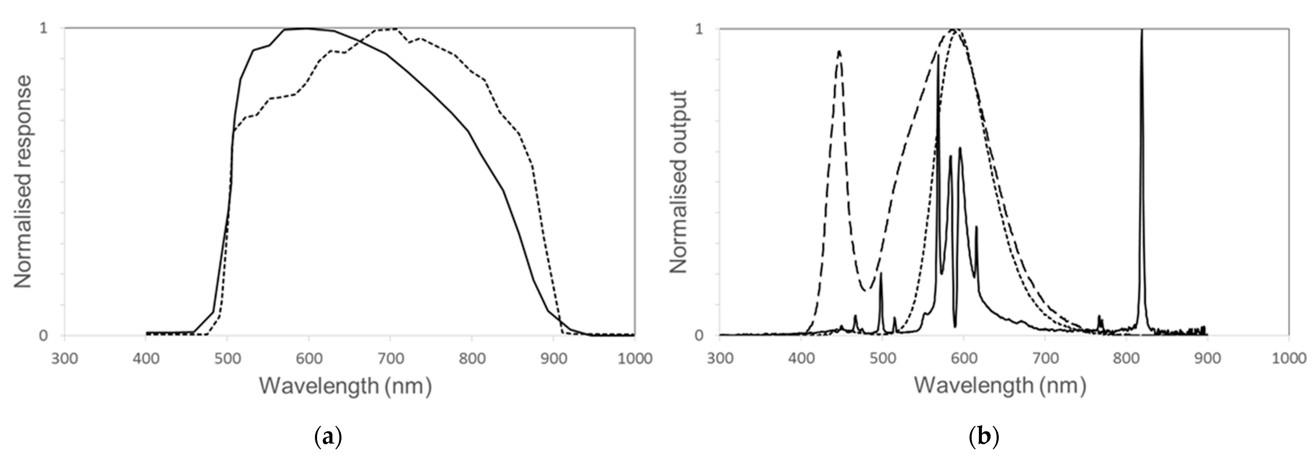
2.5. Adjusting Data for Increased Emission of Blue Light from LEDs

To estimate the effect of conversion from gas-discharge street lighting (such as high- or low-pressure sodium lamps) to solid-state lighting (LED) on our reconstructed time series, we adjusted the data post-2007 (prior to which LED lighting was not widely adopted) to estimate the radiance as perceived by the human eye, as opposed to detected by the satellite sensor. To estimate possible rates of conversion we used a post-2007 rate of replacement of gas-discharge street lighting equivalent to that recorded by the Spanish street lighting manufacturers association, Asociacion Espanola de Fabricantes de Iluminacion (ANFALUM) [44]. As a low range estimate, we assume that sodium lighting is replaced with LEDs at a correlated colour temperature (CCT) of 2000 K, with low levels of blue light, similar detectability to sodium lighting and broadly equivalent to continued use of sodium discharge lighting. As a mid-range estimate, replacement is assumed to be with LEDs with a CCT of 3000 K, the maximum recommended by the International Dark Sky Association (IDA) until 2020 and other organizations such as the European Joint Research Centre [45] or the Government of France [46]. As a high-end estimate we assume that gas- discharge lighting is progressively replaced by blue-rich LED lighting at a CCT of 4000 K. In all scenarios we assume that sodium lights are replaced after 24,000 h of continuous operation and are used for 4100 h per year. In order to estimate the emissions in the blue part of the spectrum, we used the Nikon Blue Band [24]. This is currently the only observation band available on a large scale through images acquired from the International Space Station [24]. To convert from the VIIRS-DMSP power to the Nikon Blue band, the 2000 K flux needs to be multiplied by 0.1, 3000 K by 0.25, and 4000 K by 0.5. These conversion factors were calculated using the procedures described in [24].

2.6. Details of the Method, Limitations, and Validation

This method uses the energy consumption of the street lighting of provinces of Italy as a proxy for light emissions. We do not assume that all the lights visible are streetlights, and by utilising residuals from the linear relationship between energy consumption and detected radiance we explicitly allow for a component of detected light that does not come from street lighting (step (ii) in Section 2.3 above). Previous studies have shown that trends in street lighting energy consumption are often reasonable proxies of trends in detected radiance [2,33]. Nevertheless, the residuals fitted for each province allow for local variation in the magnitude of other lighting (for example domestic and industrial sources). The street lighting energy consumption was used as a reference for the trend in growth in lighting (the slope of the regression) but this trend was offset by a fitted residual (the intercept) that can be considered an estimate of a fixed proportion of lighting from other sources. Additional validation and intermediate products can be found on Figures S6–S8 and on the data availability statement.

The proportion of night-time lighting that derives from streetlights is unclear and debated in the literature; it is likely to vary regionally between countries and cities ([7] compile different values that range from 12% in Flagstaff, AZ, USA to nearly 100% in Spain).

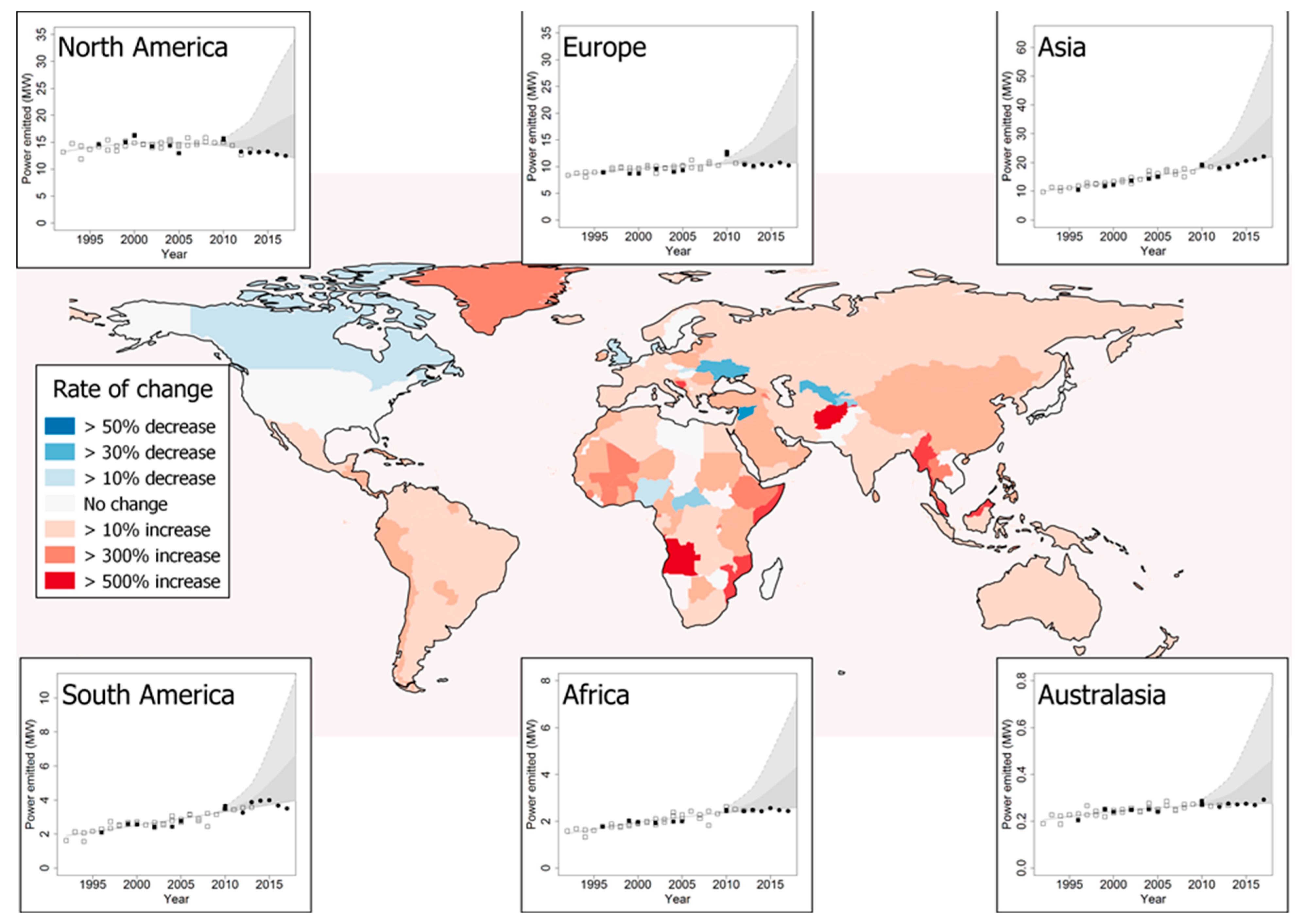
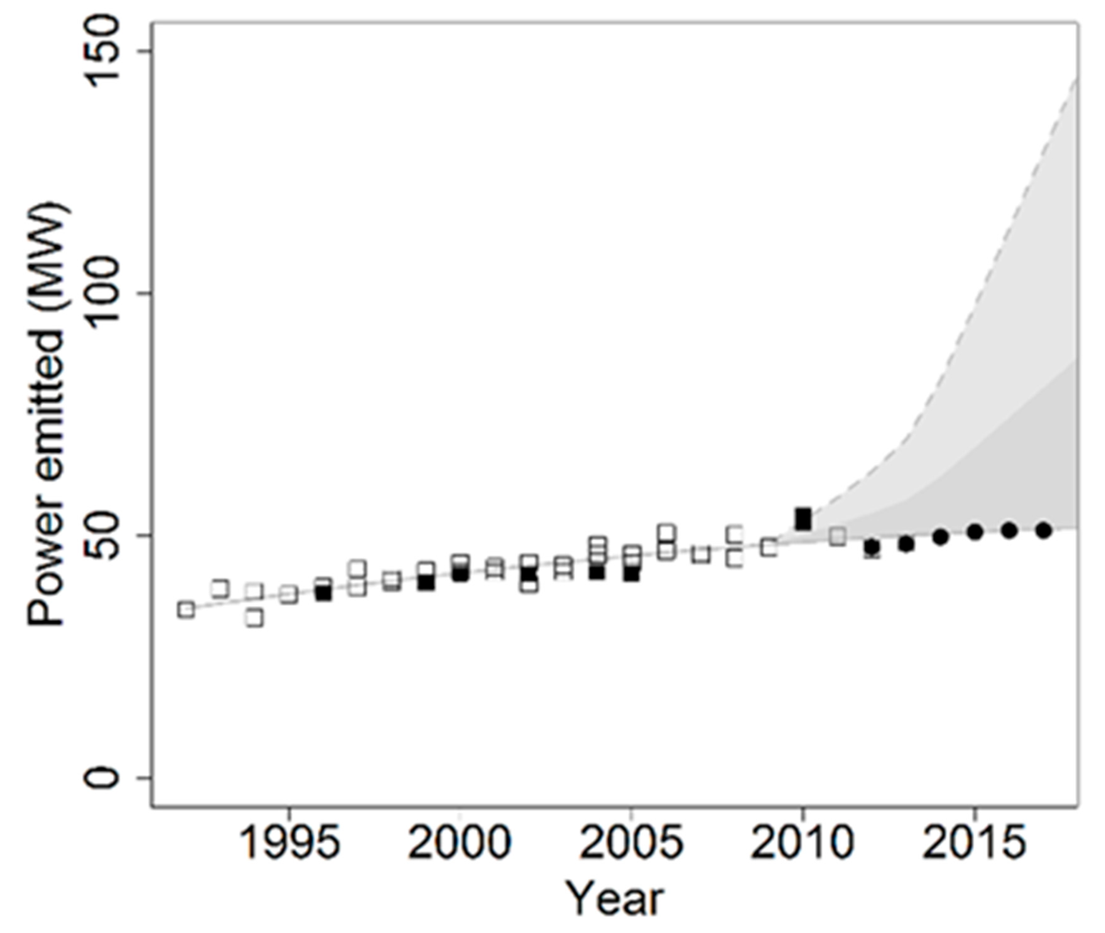
3. Results and Discussion

Globally, our analysis shows that satellite detectable light has increased at an approximately constant rate from 1992 to 2017, and by 49% over the 25 years (Figure 2). Utilising data of typical conversion and replacement rates to estimate the possible fraction of undetected light assuming different scenarios of uptake and replacement of gas-discharge lighting with LEDs, suggests however that there has been a marked recent acceleration to global emitted power (Figure 2). The projected blue light global total emission of 513 MW in 2017 would be as high as 806 MW if globally 40% of lighting were LEDs with a colour temperature of 3000 K, and 1294 MW at a colour temperature of 4000 K. Thus, not only did the “lighting revolution” associated with the transition to solid-state technology fail to result in the intended reduction in energy consumption and instead led to a rebound effect of increased use [29], but it actually resulted in a dramatic rise in that consumption compared with that which had previously been occurring. Such a recent global acceleration has also been seen in other emerging drivers of environmental change such as plastic waste production [47], and synthetic chemicals, including pesticides [48]. This raises the prospect that this change becomes increasingly challenging to redress, especially if previously unrealised synergies between the impacts of drivers emerge.

At the continental scale, persistent rates of growth in detected light are observed in Asia, South America, Oceania and Africa; while in Europe, detected light increased until around 2010 and the levelled off, and in North America it appears to be in decline (Figure 3). This is consistent with other global analyses of lighting, showing rapid urbanisation and economic growth in developing countries, and some evidence of a slowing down or decrease in light intensity in some developed nations [49]. Some proportion of this apparent lack of growth may be attributed to a saturation effect, as few remaining areas are unlit; there may also be observable effects of the decline of extractive industries [26], and better lighting design, resulting in less light being emitted above the horizontal plane. However, any conclusions as to the apparent levelling off or decrease in lighting intensity in Europe and North America should be treated with caution as the shifting spectral distribution of light towards blue-rich LEDs is likely to mask the effects of increases [49].

At the country scale, marked patterns of a decrease and increase in detected emitted power of lighting are often related to countries in conflict or recovering from conflict during this period (Figure 2); Syria [1], Ukraine [50], Central African Republic, and Yemen [51] (see Figure S9) all show marked decreases in emitted power of lighting over the period, while Bosnia and Herzegovina, Afghanistan, Angola, Mozambique and Somalia all show decreases. Declines in Nigeria and Uzbekistan are apparently due, in large part, to changes in light emissions in areas of oil extraction.

The recent growth, and relative uncertainty in the scale of global emissions of low wavelength blue light is significant as lower wavelengths of visible light are implicated in the disruption of circadian rhythms in humans and other animals and have been shown to be more effective than longer wavelengths at driving a range of ecological responses, from phototaxis in insects to disrupting reproduction in mammals [49]. This highlights the need for multispectral nighttime imagery to monitor the ongoing changes in the spectral composition of artificial light in the environment as technology changes, as well as the creative use of multiple data sources to reconstruct the changing spectral signature of nocturnal lightscapes in the past.

4. Conclusions

Despite decades of remote sensing of night-time lights, reconstructing recent global trends in light pollution remains challenging due to the lack of calibration and saturation of the early DMSP-OLS datasets, the lack of spectral information from panchromatic sensors, and the relatively poor sensitivity of existing satellite sensors to blue light. This analysis places bounds on the uncertainty in global trends in nocturnal power emissions by combining remote sensing data from different sources with power consumption data from municipal street lighting. While considerable uncertainty remains, it is clear that light emissions have increased by at least 49% over the 25-year period studied, and that this estimate is likely to be conservative; the transition to blue-rich solid-state LED lighting likely masks a much larger increase that is under-detected by existing panchromatic satellite data.

References

1. Levin, N.; Kyba, C.C.M.; Zhang, Q.; Sánchez, M.A.; Miguel, O.; Román, M.O.; Li, X.; Portnov, B.A.; Molthan, A.L.; Jechow, A.; et al. Remote sensing of night lights: A review and an outlook for the future. Remote. Sens. Environ. 2020, 237, 111–443. [Google Scholar] [CrossRef]
2. Bennie, J.; Davies, T.W.; Duffy, J.P.; Inger, R.; Gaston, K.J. Contrasting trends in light pollution across Europe based on satellite observed night time lights. Sci. Rep. 2015, 4, 3789. [Google Scholar] [CrossRef] [Green Version]
3. Bustamante-Calabria, M.; Sánchez, M.A.; Martín-Ruiz, S.; Ortiz, J.L.; Vílchez, J.M.; Pelegrina, A.; García, A.; Zamorano, J.; Bennie, J.; Gaston, K.J. Effects of the COVID-19 lockdown on urban light emissions: Ground and satellite comparison. Remote Sens. 2021, 13, 258. [Google Scholar] [CrossRef]
4. Small, C.; Pozzi, F.; Elvidge, C.D. Spatial analysis of global urban extent form DMSP-OLS night lights. Remote. Sens. Environ. 2005, 96, 277–291. [Google Scholar] [CrossRef]
5. Elvidge, C.D.; Sutton, P.C.; Ghosh, T.; Tuttle, B.T.; Baugh, K.E.; Bhaduri, B.; Bright, E. A global poverty map derived from satellite data. Comput. Geosci. 2009, 35, 1652–1660. [Google Scholar] [CrossRef]
6. Cinzano, P.; Falchi, F.; Elvidge, C.D. The first world atlas of artificial night sky brightness. Mon. Not. R. Astron. Soc. 2001, 328, 689–707. [Google Scholar] [CrossRef] [Green Version]
7. Kyba, C.; C, M.; Ruby, A.; Kuechly, H.U.; Kinzey, B.; Miller, N.; Sanders, J.; Barentine, J.; Kleinodt, R.; Espey, B. Direct measurement of the contribution of street lighting to satellite observations of nighttime light emissions from urban areas. Light. Res. Technol. 2021, 53, 189–211. [Google Scholar] [CrossRef]
8. Hoag, A.A.; Schoening, W.E.; Coucke, M. City sky glow monitoring at Kitt Peak. Publ. Astron. Soc. Pac. 1973, 85, 503. [Google Scholar] [CrossRef]
9. Benn, C.R.; Ellison, S.L. Brightness of the night sky over La Palma. New Astron. Rev. 1998, 42, 503–507. [Google Scholar] [CrossRef] [Green Version]
10. Garcia-Saenz, A.; Sánchez, M.A.; Espinosa, A.; Valentín, A.; Aragonés, N.; Llorca, J.; Amiano, P.; Sánchez, V.M.; Guevara, M.; Capelo, R.; et al. Evaluating the association between artificial light-at-night exposure and breast and prostate cancer risk in Spain (MCC-Spain study). Environ. Health Persp. 2018, 126, 047011. [Google Scholar] [CrossRef] [PubMed]
11. Kloog, I.; Stevens, R.G.; Haim, A.; Portnov, B.A. Nighttime light level co-distributes with breast cancer incidence worldwide. Cancer Causes Control 2010, 21, 2059–2068. [Google Scholar] [CrossRef]
12. Owens, A.; Cochard, P.; Durrant, J.; Farnworth, B.; Perkin, E. Light pollution as a driver of insect declines. Biol. Conserv. 2020, 241, 108259. [Google Scholar] [CrossRef]
13. Eisenbeis, G.; Hänel, A.; McDonnell., J.M.; Hahs, A.; Breuste, J. Light pollution and the impact of artificial night lighting on insects. In Ecology of Cities and Towns: A comparative approach; Cambridge University Press: New York, NY, USA, 2009; pp. 243–263. [Google Scholar]
14. Sanders, D.; Gaston, K.J. How ecological communities respond to artificial light. J. Exp. Zool. A 2018, 329, 394–400. [Google Scholar] [CrossRef] [PubMed] [Green Version]
15. Longcore, T.; Rich, C. Ecological light pollution. Front. Ecol. Environ. 2004, 2, 191–198. [Google Scholar] [CrossRef]
16. Knop, E.; Zoller, L.; Ryser, R.; Gerpe, C.; Hörler, M.; Fontaine, C. Artificial light at night as a new threat to pollination. Nature 2017, 548, 206–209. [Google Scholar] [CrossRef]
17. Altermatt, F.; Ebert, D. Reduced flight-to-light behaviour of moth populations exposed to long-term urban light pollution. Biol. Lett. 2016, 12, 4. [Google Scholar] [CrossRef]
18. Elvidge, C.D.; Hsu, F.C.; Baugh, K.E.; Ghosh, T. National trends in satellite observed lighting: 1992–2012. In Global Urban Monitoring and Assessment through Earth Observation; Weng, Q., Ed.; CRC Press: Boca Raton, FL, USA, 2014. [Google Scholar]
19. Kyba, C.C.M.; Kuester, T.; Sánchez, M.A.; Baugh, K.; Jechow, A.; Hölker, F.; Bennie, J.; Elvidge, C.D.; Gaston, K.J.; Guanter, L. Artificially lit surface of Earth at night increasing in radiance and extent. Sci. Adv. 2017, 3, e1701528. [Google Scholar] [CrossRef] [Green Version]
20. Imhoff, M.L.; Lawrence, W.T.; Stutzer, D.C.; Elvidge, C.D. A technique for using composite DMSP/OLS “City Lights” satellite data to map urban area. Remote Sens. Environ. 1997, 6, 361–370. [Google Scholar] [CrossRef]
21. Tuttle, B.T.; Anderson, S.; Elvidge, C.D.; Tilottama, G.; Baugh, K.; Baugh, K.; Sutton, P.C. Aladdin’s magic lamp: Active target calibration of the DMSP OLS. Remote Sens. 2014, 6, 12708–12722. [Google Scholar] [CrossRef] [Green Version]
22. Sánchez, M.A.; Kyba, C.C.; Zamorano, J.; Gallego, J.; Gaston, K.J. The nature of the diffuse light near cities detected in nighttime satellite imagery. Sci. Rep. 2020, 10, 1–16. [Google Scholar]
23. Elvidge, C.D.; Baugh, K.E.; Zhizhin, M.; Hsu, F.C. Why VIIRS data are superior to DMSP for mapping nighttime lights. Proc. Asia-Pacific. Adv. Netw. 2013, 35, 62–69. [Google Scholar]
24. Sánchez, M.A.; Kyba, C.C.M.; Aube, M.; Zamorano, J.; Cardiel, N.; Tapia, C.; Bennie, J.; Gaston, K.J. Colour remote sensing of the impact of artificial light at night (I): The potential of the International Space Station and other DSLR-based platforms. Remote Sens. Environ. 2019, 224, 92–103. [Google Scholar] [CrossRef]
25. Zheng, Q.; Weng, Q.; Huang, L.; Wang, K.; Deng, J.; Jiang, R.; Ye, Z.; Gan, M. A new source of multi-spectral high spatial resolution night-time light imagery—JL1-3B. Remote Sens. Environ. 2018, 215, 300–312. [Google Scholar] [CrossRef]
26. Wu, J.; He, S.; Peng, J.; Li, W.; Zhong, X. Intercalibration of DMSP-OLS night-time light data by the invariant region method. Int. J. Remote Sens. 2013, 34, 7356–7368. [Google Scholar] [CrossRef]
27. Pandey, B.; Zhang, Q.; Seto, K.C. Comparative evaluation of relative calibration methods for DMSP/OLS nighttime lights. Remote Sens. Environ. 2017, 195, 67–78. [Google Scholar] [CrossRef]
28. Ryan, R.E.; Pagnutti, M.; Burch, K.; Leigh, L.; Ruggles, T.; Cao, C.Y.; Aaron, D.; Blonski, S.; Helder, D. The Terra Vega active light source: A first step in a new approach to perform absolute radiometric calibrations and early results calibrating the VIIRS DNB. Remote Sens. 2019, 11, 710. [Google Scholar] [CrossRef] [Green Version]
29. Hsu, F.; Baugh, K.E.; Ghosh, T.; Zhizhin, M.; Elvidge, C.D. DMSP-OLS radiance calibrated nighttime lights time series with intercalibration. Remote Sens. 2015, 7, 1855–1876. [Google Scholar] [CrossRef] [Green Version]
30. SpA, T. Statistical Data on Electricity in Italy (‘in Italian’). Available online: http://www.terna.it (accessed on 20 August 2021).
31. Elvidge, C.D.; Ziskin, D.; Baugh, K.E.; Tuttle, B.T.; Ghosh, T.; Pack, D.; Erwin, E.H.; Zhizhin, M.N. A fifteen year record of global natural gas flaring derived from satellite data. Energies 2009, 2, 595–622. [Google Scholar] [CrossRef]
32. Li, X.; Zhao, L.; Li, D.; Xu, H. Mapping urban extent using Luojia 1-01 nighttime light imagery. Sensors 2018, 11, 3665. [Google Scholar] [CrossRef] [PubMed] [Green Version]
33. Sánchez, M.A.; Zamorano, J.; Gómez, C.J.; Pascual, S. Evolution of the energy consumed by Street lighting in Spain estimated with DMSP-OLS data. J. Quant. Spectrosc. Rad. 2014, 139, 109–117. [Google Scholar] [CrossRef] [Green Version]
34. Zhang, Q.; Pandey, B.; Seto, K.C. A robust method to generate a consistent time series from DMSP/OLS nighttime light data. IEEE T. Geosci. Remote 2016, 54, 5821–5831. [Google Scholar] [CrossRef]
35. Xiong, X.; Wilson, T.; Angal, A.; Sun, J. Using the moon and stars for VIIRS day/night band on-orbit calibration. P. Soc. Photo-Opt. Ins 2019, 11151, 111511Q. [Google Scholar]
36. R Core Team. Available online: https://www.R-project.org/ (accessed on 20 August 2021).
37. Gorelick, N.; Hancher, M.; Dixon, M.; Llyushchenko., S.; Thau, D.; Moore., R. Google Earth Engine: Planetary-scale geospatial analysis for everyone. Remote Sens. Environ. 2017, 202, 18–27. [Google Scholar] [CrossRef]
38. Harris, C.R.; Millman, K.J.; Van der Walt, S.J.; Gommers, R.; Virtanen, P.; Cournapeau, D.; Wieser, E.; Taylor, J.; Berg, S.; Smith, N.J.; et al. Array programming with NumPy. Nature 2020, 585, 357–362. [Google Scholar] [CrossRef] [PubMed]
39. Robitaille, T.P.; Tollerud, E.J.; Greenfield, P.; Droettboom, M.; Bray, E.; Aldcroft, T.; Davis, M.; Ginsburg, A.; Price-Whelan, A.M.; Kerzendorf, W.E.; et al. Astropy: A community Python package for astronomy. Astron. Astrophys. 2013, 558, A33. [Google Scholar]
40. McKinney, W. Available online: https://bit.ly/3gkRhGD (accessed on 20 August 2021).
41. Virtanen, P.; Gommers, R.; Oliphant, T.E.; Haberland, M.; Reddy, T.; Cournapeau, D.; Burovski, E.; Peterson, P.; Weckesser, W.; Bright, J.; et al. SciPy 1.0: Fundamental algorithms for scientific computing in Python. Nat. Methods 2020, 17, 261–272. [Google Scholar] [CrossRef] [PubMed] [Green Version]
42. Hunter, J.D. Matplotlib: A 2D graphics environment. Comput. Sci. Eng. 2007, 9, 90–95. [Google Scholar] [CrossRef]
43. Salunke, S.S. Selenium Webdriver in Python: Learn with Examples; CreateSpace Independent Publishing Platform: Scotts Valley, CA, USA, 2014. [Google Scholar]
44. Anfalum. Available online: https://bit.ly/3gj9Hrd (accessed on 20 August 2021).
45. Donatello, S.; Quintero, R.R.; Caldas, M.G.; Wolf, O.; Van, T.P.; Van, H.V.; Geerken, T. Revision of the EU Green Public Procurement Criteria for Road Lighting and Traffic Signals; Publications Office of the European Union: Luxembourg, 2009. [Google Scholar]
46. Legifrance. Available online: https://bit.ly/3851LVX (accessed on 20 August 2021).
47. Geyer, R.; Jambeck, J.R.; Law, K.L. Production, use and fate of all plastic ever made. Sci. Adv. 2017, 3, e1700782. [Google Scholar] [CrossRef] [PubMed] [Green Version]
48. Bernhardt, E.S.; Rosi, E.J.; Gessner, M.O. Synthetic chemicals as agents of global change. Front. Ecol. Environ. 2017, 15, 84–90. [Google Scholar] [CrossRef]
49. Longcore, T.; Rodriguez, A.; Witherington, B.; Penniman, J.F.; Herf, L.; Herf, M. Rapid assessment of lamp spectrum to quantify ecological effects of light at night. J. Exp. Zool. A 2018, 329, 511–521. [Google Scholar] [CrossRef]
50. Lyalko, V.; Apostolov, A.; Yelistratova, L.; Khodorovsky, A. The assessment of the social-economic elaboration of the Ukraine in independent years within the DMSP/OLS satellite data about the night lighting. Ukrainian. J. Remote Sens. 2018, 16, 27–33. [Google Scholar]
51. Jiang, W.; He, G.; Long, T.; Liu, H. Ongoing conflict makes Yemen dark: From the perspective of nighttime light. Remote Sens. 2017, 9, 798. [Google Scholar] [CrossRef] [Green Version]
Figure 1. Typical normalized spectral response of satellite sensors and selected streetlighting types. (a) the DMSP-OLS (solid line) and VIIRS-DNB (dashed line) sensors, compared with (b) normalized output of high pressure sodium (solid line), 1800 K LED (short dashes) and 4000 K LED (long dashes) streetlights.
Remotesensing 13 03311 g001
Figure 2. Rate of change in artificial light at night represented as power output detectable by satellites from 1992 to 2017 assessed across countries (map) and continents (inset plots). In plots, open squares represent annual DMSP-OLS composite data, filled squares represent radiance calibrated DMSP-OLS data, filled circles represent VIIRS Day/Night band data. Plotted data points show satellite data assuming constant spectral composition of light emissions. The shaded areas represent the possible range of undetected light assuming a recent phased transition from high pressure sodium lighting to LEDs of color temperature 3000 K (dark grey) or 4000 K (light grey).
Remotesensing 13 03311 g002
Figure 3. Global emitted power (Nikon blue band [14]) detected by satellites from artificial light sources from 1992 to 2017. Open squares represent annual DMSP-OLS composite data, filled squares represent radiance calibrated DMSP-OLS data, filled circles represent VIIRS Day/Night band data. Plotted data points assume constant spectral composition of light emissions. The shaded areas represent the possible range of undetected light assuming a recent phased transition from high pressure sodium lighting to LEDs of color temperature 3000 K (dark grey) or 4000 K (light grey).
Remotesensing 13 03311 g003
Publisher’s Note: MDPI stays neutral with regard to jurisdictional claims in published maps and institutional affiliations.