Article

Quad-FPN: A Novel Quad Feature Pyramid Network for SAR Ship Detection

School of Information and Communication Engineering, University of Electronic Science and Technology of China, Chengdu 611731, China
*
Author to whom correspondence should be addressed.
Remote Sens. 2021, 13(14), 2771; https://doi.org/10.3390/rs13142771
Submission received: 26 May 2021 / Revised: 25 June 2021 / Accepted: 2 July 2021 / Published: 14 July 2021
(This article belongs to the Special Issue Advances in Object and Activity Detection in Remote Sensing Imagery)

Abstract

:
Ship detection from synthetic aperture radar (SAR) imagery is a fundamental and significant marine mission. It plays an important role in marine traffic control, marine fishery management, and marine rescue. Nevertheless, there are still some challenges hindering accuracy improvements of SAR ship detection, e.g., complex background interferences, multi-scale ship feature differences, and indistinctive small ship features. Therefore, to address these problems, a novel quad feature pyramid network (Quad-FPN) is proposed for SAR ship detection in this paper. Quad-FPN consists of four unique FPNs, i.e., a DEformable COnvolutional FPN (DE-CO-FPN), a Content-Aware Feature Reassembly FPN (CA-FR-FPN), a Path Aggregation Space Attention FPN (PA-SA-FPN), and a Balance Scale Global Attention FPN (BS-GA-FPN). To confirm the effectiveness of each FPN, extensive ablation studies are conducted. We conduct experiments on five open SAR ship detection datasets, i.e., SAR ship detection dataset (SSDD), Gaofen-SSDD, Sentinel-SSDD, SAR-Ship-Dataset, and high-resolution SAR images dataset (HRSID). Qualitative and quantitative experimental results jointly reveal Quad-FPN’s optimal SAR ship detection performance compared with the other 12 competitive state-of-the-art convolutional neural network (CNN)-based SAR ship detectors. To confirm the excellent migration application capability of Quad-FPN, the actual ship detection in another two large-scene Sentinel-1 SAR images is conducted. Their satisfactory detection results indicate the practical application value of Quad-FPN in marine surveillance.

Graphical Abstract

1. Introduction

Synthetic aperture radar (SAR) is an advanced active microwave sensor for the high-resolution remote sensing observation of the Earth [1]. Its all-day and all-weather working capacity makes it play an important role in marine surveillance [2]. As a fundamental marine mission, SAR ship detection is of great value in marine traffic control, fishery management, and emergent salvage at sea [3,4]. Thus, up to now, the topic of SAR ship detection has received continuous attention from an increasing number of scholars [5,6,7,8,9,10,11,12,13,14,15].
In earlier years, a standard solution is to design ship features by manual ways, e.g., constant false alarm rate (CFAR) [1], saliency [2], super-pixel [3], and transformation [4]. Yet, these traditional methods are always complex in algorithm, weak in migration, and cumbersome in manual design, leading to their limited migration applications. Moreover, they often use limited ship images for theoretical analysis to define ship features, but these features cannot reflect the characteristics of ships with various sizes under different backgrounds. This causes their poor multi-scale and multi-scene detection performance.
Fortunately, in recent years, with the rise of deep learning (DL) and convolutional neural networks (CNNs), current state-of-the-art DL-based/CNN-based SAR ship detectors have helped solve the above-mentioned problems, to some degree. Compared with traditional methods, CNN-based ones have significant advantages, i.e., simplicity, high-efficiency, and high-accuracy, because they can enable computational models with multiple processing layers to learn data representations with multiple-level abstractions. This can effectively improve detection accuracy. Thus, nowadays, many scholars [5,6,7,8,9,10,11,12,13,14,15] in the SAR ship detection community are starting to pay much attention to CNN-based methods.
For instance, based on Fast R-CNN [16], Li et al. [9] proposed a binarized normed gradient-based method to extract SAR ship-like regions. Based on Faster R-CNN [17], Lin et al. [14] designed a squeeze and excitation rank mechanism to improve detection performance. Based on you only look once (YOLO) [18], Zhang et al. [10] integrated the multi-scale mechanism, concatenation mechanism, and anchor box mechanism for small ship detection. Based on RetinaNet [19], Yang et al. [11] tried to suppress ship detections’ false alarms by loss weighting means. Based on single shot multi-box detector (SSD) [20], Wang et al. [7] proposed an optimized version to enhance small ship detection while improving detection speed. Based on Cascade R-CNN [21], Wei et al. [12] designed a robust SAR ship detector named HR-SDNet for multi-level ship feature extraction.
Since the feature pyramid network (FPN) was proposed by Lin et al. [22], it has been a standard solution for multi-scale SAR ship detection. For different resolutions, incident angles, satellites, etc., SAR ships possess various sizes. FPN can detect ships with different sizes at different resolution levels based on more reasonable semantic features from backbone networks. This enables better detection performance. Thus, it has received a wide range of attention, e.g., Wei et al. [12] optimized its structure to present a high-resolution FPN for better multi-scale detection. Cui et al. [13] adopted a convolutional block attention module to improve its performance. Lin et al. [14] added a squeeze-and-excitation module at the top of FPN to activate important features. Zhao et al. [15] designed an attention receptive pyramid network to detect ships with various sizes and complex backgrounds.
However, SAR ship detection is still a challenging issue due to complex background interferences (e.g., port facilities, sea clutters, and volatile sea states), multi-scale ship feature differences, and indistinctive small ship features. Thus, this paper proposes a novel quad feature pyramid network (Quad-FPN) for SAR ship detection. Figure 1 shows Quad-FPN’s structure. From Figure 1, four FPNs constitute it, i.e., a DEformable COnvolutional FPN (DE-CO-FPN), a Content-Aware Feature Reassembly FPN (CA-FR-FPN), a Path Aggregation Space Attention FPN (PA-SA-FPN), and a Balance Scale Global Attention FPN (BS-GA-FPN). Their implementation shows a pipeline, meaning gradually enhancing detection performance. We conduct extensive ablation studies to confirm each FPN’s effectiveness. Experimental results on five open SAR ship detection datasets (i.e., SSDD [5], Gaofen-SSDD [6], Sentinel-SSDD [6], SAR-Ship-Dataset [7], and HRSID [8]) reveal that Quad-FPN can offer the most superior detection accuracy compared with the other 12 competitive state-of-the-art CNN-based SAR ship detectors. Finally, we also perform the actual ship detection in another two large-scene SAR images from the Sentinel-1 satellite. The satisfactory detection results confirm the excellent migration application capability of Quad-FPN. The software is available online on our website [23].
The main contributions of this paper are as follows:
  • Quad-FPN is proposed for SAR ship detection.
  • DE-CO-FPN, CA-FR-FPN, PA-SA-FPN, and BS-GA-FPN are designed to improve SAR ship detection performance.
  • Quad-FPN offers the most superior detection accuracy compared with the other 12 competitive state-of-the-art CNN-based SAR ship detectors.
The rest of this paper is arranged as follows. Section 2 introduces Quad-FPN. Section 3 introduces our experiments. Results are shown in Section 4. Ablation studies are presented in Section 5. Finally, a summary of this paper is made in Section 6.

2. Quad-FPN

Quad-FPN is the basis of classical Faster R-CNN [17] and FPN [22], which are both important solutions to handle mainstream detection tasks. Figure 2 shows Quad-FPN’s overview. Four basic FPNs, i.e., DE-CO-FPN, CA-FR-FPN, PA-SA-FPN, and BS-GA-FPN, constitute its network architecture. Their implementation presents a pipeline that improves SAR ship detection performance progressively.
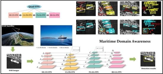
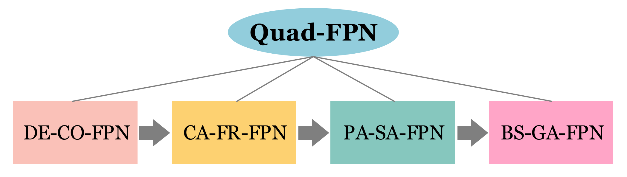
The overall design idea of Quad-FPN is as follows.
(1)
The overall structure of the first two FPNs (DE-CO-FPN and CA-FE-FPN) keeps the same as that of the raw FPN [22], including the sequence of DE-CO-FPN and CA-FE-FPN. In other words, the raw FPN also has two basic sub-FPNs, but they are replaced by our proposed DE-CO-FPN and CA-FE-FPN. Differently, the first sub-FPN in the raw FPN uses the standard convolution, but DE-CO-FPN uses the deformable convolution; the second sub-FPN in the raw FPN uses the simple up-sampling to achieve a feature fusion, but CA-FE-FPN proposes a CA-FR-Module to achieve a feature fusion. DE-CO-FPN’s feature maps are from the backbone network, so it is located at the input-end of Quad-FPN. From Figure 2a, DE-CO-FPN realizes the information flow from the bottom to the top. According to the findings in [22], the pyramid top (A5) has stronger semantic information than its low levels. The semantic information can improve detection performance. Therefore, a top-to-bottom branch in CA-FR-FPN is added to achieve the downward transmission of semantic information. Finally, DE-CO-FPN and CA-FE-FPN form an information interaction loop in which spatial location information and semantic information complement each other.
(2)
The design idea of the third FPN (PA-SA-FPN) is inspired from the work of PANET They found that the low-level location information of the pyramid bottom (B5) was not considered to be transmitted to the top. This might lead to an inaccurate positioning of large objects, so the detection performance of large objects is reduced. Therefore, they added an extra bottom-to-top branch to address this problem. This branch is called PA-FPN in their original reports. Differently, our proposed PA-SA-FPN adds a PA-SA-Module to achieve the feature down-sampling so as to focus on more important spatial features. Finally, CA-FE-FPN and PA-SA-FPN form another information interaction loop in which spatial location information and semantic information complement each other again. Therefore, the overall sequence of DE-CO-FPN, CA-FE-FPN, and PA-SA-FPN is fixed.
(3)
The basic outline of Quad-FPN has been determined. BS-GA-FPN is designed to further refine features at each feature level to solve the feature level imbalance of different scale ships. Thus, it is arranged at the output-end of Quad-FPN.

2.1. DEformable COnvolutional FPN (DE-CO-FPN)

The core idea of DE-CO-FPN is that we use the deformable convolution [24] to extract ship features. It contains more useful ship shape information, meanwhile alleviating complex background interferences. Previous work [5,6,7,8,9,10,11,12,13,14,15] mostly adopted the standard or dilated convolutions [25] to extract features. However, the two have limited geometric modeling ability due to their regular kernels. This means that their ability to extract the shape features of multi-scale ships is bound to become poor, causing poor multi-scale detection performance. For inshore ships, the standard and dilated convolutions cannot restrain interferences of port facilities; for ships side-by-side parking at ports, they also cannot eliminate interferences from the nearby ship hull. Thus, to solve this problem, the deformable convolution is used to establish DE-CO-FPN. 
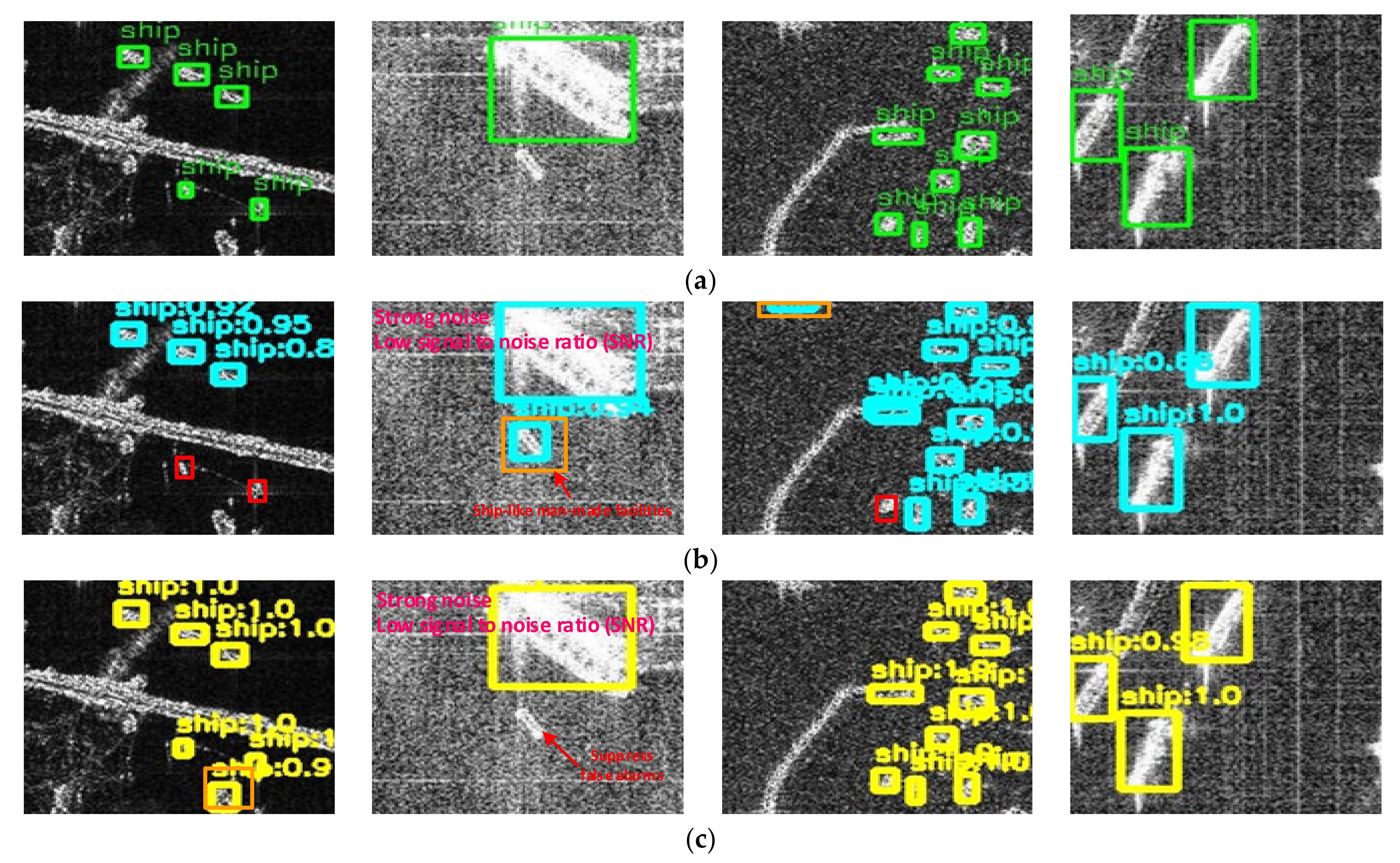
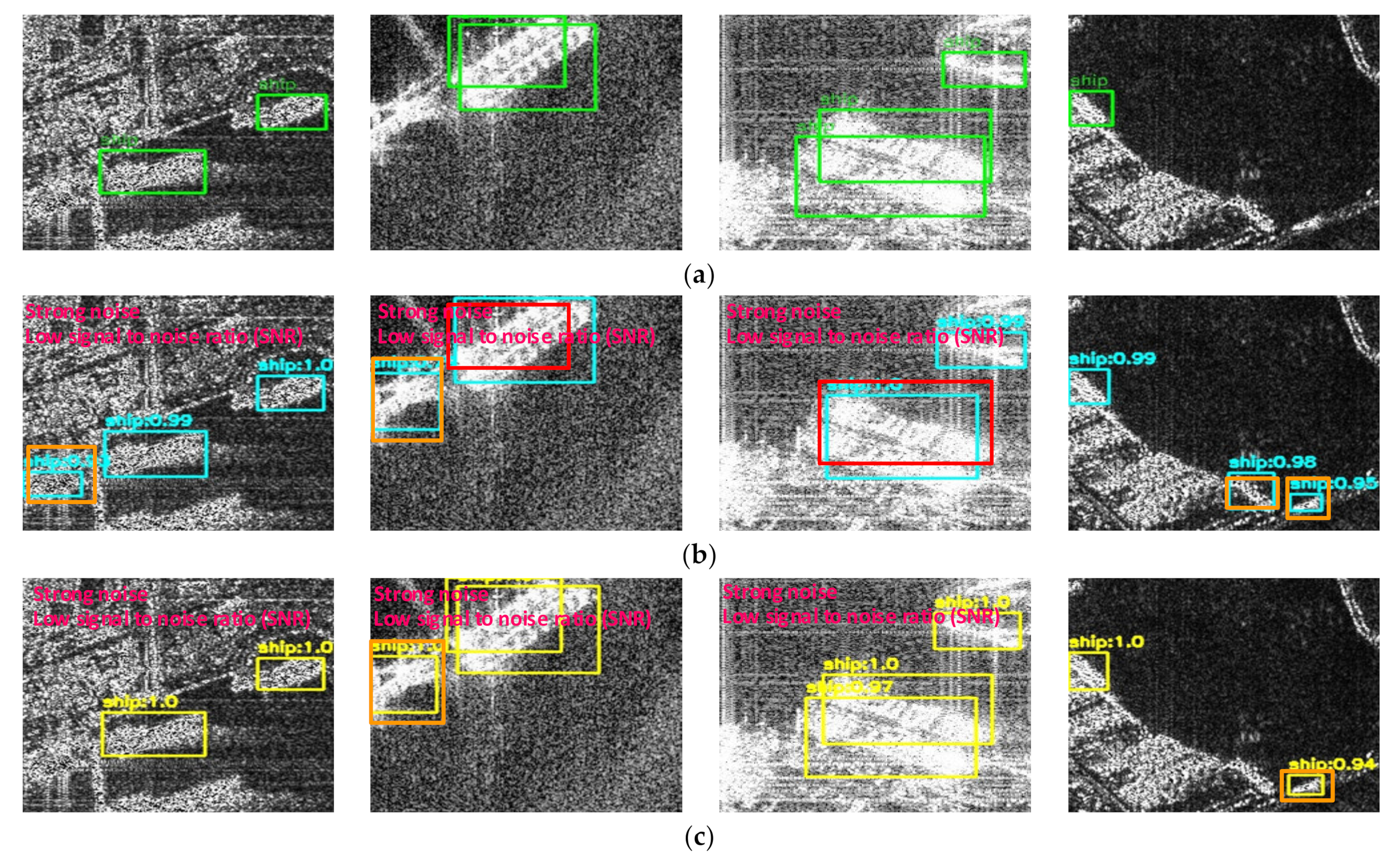
Figure 3 shows their intuitive comparison. From Figure 3, it is obvious that the deformable convolution can extract ship shape features more effectively; it can suppress the interference of complex backgrounds, especially for more complex inshore scenes. Finally, ships are likely to be separated successfully from complex backgrounds. Thus, this deformable convolution process can be regarded as an extraction of salient objects in various scenes, which plays a role of spatial attention.
In the deformable convolution, the standard convolution kernel is augmented with offsets ∆pn that are adaptively learned in training to model targets’ shape features, i.e.,
y p 0 = p n w p n × x p 0 + p n + Δ p n
where p0 denotes each location, ℜ denotes the convolution region, w denotes the weight parameters, x denotes the input, y denotes the output, and ∆pn denotes the learned offsets at the n-th location. It should be noted that compared with standard convolutions, deformable ones’ training is in fact time-consuming; it needs more GPU memory. This is because the learned offsets add extra network parameters, increasing networks’ complexity. A reasonable fitting of these offsets must be time-consuming. Yet, in this paper, to obtain better accuracy of ships with various shapes, we have not studied this issue deeply for the time being. This problem will be considered with due attention in our future work.
In Equation (1), ∆pn is typically fractional. Thus, we use the bilinear interpolation to ensure the smooth implementation of convolutions, i.e.,
x p = q G q , p × x q
where p denotes the fraction location to be interpolated, q denotes all integral spatial locations in the feature map x, and G( ) denotes the bilinear interpolation kernel defined by
G q , p = g q x , p x × g q y , p y ,   w h e r e   g a , b = max 0 , 1 a b
In experiments, we add another one convolution layer to learn the offsets ∆pn. Then, the standard convolution combining ∆pn is performed on the input feature maps. Finally, ship features with rich shape information (A1, A2, A3, A4, and A5 in Figure 2a) will be transferred to subsequent FPNs for more operations.

2.2. Content-Aware Feature Reassembly (CA-FR-FPN)

The core idea of CA-FR-FPN is that we design a CA-FR-Module (marked by circle in Figure 2b) to enhance feature transmission benefits when performing the up-sampling multi-level feature fusion. Previous work [5,6,7,8,9,10,11,12,13,14,15] added a feature fusion branch from top to bottom to via feature up-sampling. This feature up-sampling is often completed by the nearest neighbor or bilinear interpolations, but the two means merely consider sub-pixel neighborhoods, which cannot effectively capture the rich semantic information required by dense detection tasks [26], especially for densely distributed small ships. That is, features of small ships are easily diluted because of their poor conspicuousness, leading to feature loss. Thus, to solve this problem, we propose a CA-FR-Module in the up-sampling feature fusion branch from top to bottom to achieve a feature reassembly. It can be aware of important contents in feature maps, and attach importance to key small ship features, thereby improving feature transmission benefits. Figure 2b shows the network architecture of CA-FR-FPN. From Figure 2b, for five-scale levels (B1, B2, B3, B4, and B5), four CA-FR-Modules are used for feature reassembly. In practice, CA-FR-Module will complete the task that is similar to the 2× up-sampling operation in essence. Figure 4 shows the implementation process of CA-FR-Module. From Figure 4, there are two basic steps in CA-FR-Module: (1) kernel prediction, and (2) content-aware feature reassembly.
Step 1: Kernel Prediction
Figure 4a shows the implementation process of the kernel prediction. In Figure 4, the feature maps F’s dimension is L × L × C, where L denotes its size and C denotes its channel width. Overall, the process of the kernel prediction (denoted by ψ) is responsible for generating adaptive feature reassembly kernels Wl at the original location l, according to the k × k neighbors of feature maps Fl through a content-aware manner, i.e.,
W l = ψ ( N ( F l , k ) )
where N(·) means the neighbors and Wl denotes the reassembly kernel.
To enhance the content-aware benefits of the kernel prediction, we first design a convolution layer to amplify the inputted feature maps F by α times (from C to α∙C). This convolution layer’s kernel number is set to α∙C, where α is an experimental hyper-parameter that will be studied in Section 5.2.2. Then, we adopt another convolution layer to encode the content of input features so as to obtain reassembly kernels. Here, we set the kernel width as 22 × k × k where 2 is from the requirement of the 2× up-sampling operation. The purpose is to enlarge the size of feature maps to 2L. Moreover, k × k is from the k × k neighbors of feature maps Fl. Afterwards, the content encoded features are reshaped to a 2L × 2L × (k × k) dimension via the pixel shuffle means [27]. Finally, each reassembly kernel is normalized by a soft-max function spatially to reflect the weight of each sub-content.
In summary, the above operations can be described by:
W l = s o f t - m a x { s h u f f l e [ f e n c o d e ( f a m p l i f y ( F l ) ) ] }
where famplify denotes the feature amplification operation, fencode denotes the content encode operation, shuffle denotes the pixel shuffle means, soft-max denotes the soft-max function defined by e X i / j e X j , and Wl denotes the generated reassembly kernel.
Step 2: Content-Aware Feature Reassembly
Figure 4b shows the implementation process of the content-aware feature reassembly. Overall, the process of the content-aware feature reassembly (denoted by ϕ) is responsible for generating the final up-sampling feature maps Fl, i.e.,
F l = ϕ N F l , k , W l
where k denotes the k × k neighbors and Wl denotes the reassembly kernel in Equation (4) that corresponds to the l’ location of feature maps after up-sampling from the original l location. For each reassembly kernel Wl, this step will reassemble the features within a local region via the function ϕ in Equation (6). Similar to the standard convolution operation, ϕ can be implemented by a weighted sum. Thus, for a target location l’ and the corresponding square region N(Fl, k) centered at l = (i, j), the reassembly output is described by
F l = n , m W l , ( n , m ) × F ( i + n , j + m )
where ℜ denotes the corresponding square region N(Fl, k). Moreover, k is set to 5 in our work that is an optimal value followed by [26].
With the reassembly kernel Wl, each pixel in the region ℜ of the original location l contributes to the up-sampled pixel l′ differently, based on the content of features rather than location distance. Semantic features from the pyramid top will be transferred into the bottom, bringing better transmission benefits. Finally, the pyramid top’s features will be fused into the bottom to enhance the feature expression ability of small ships.

2.3. Path Aggregation Space Attention FPN (PA-SA-FPN)

The core idea of PA-SA-FPN is that we add an extra path aggregation branch with a space attention module (PA-SA-Module) (marked by circle in Figure 2c) from the pyramid bottom to the top. Previous work [5,6,7,8,9,10,11,12,13,14,15] often transmitted high-level strong semantic features to the bottom to improve the whole pyramid expressiveness. Yet, the low-level location information from the pyramid bottom was not considered to be transmitted to the top. This can lead to inaccurate positionings of large ship bounding boxes, so the detection performance of large ships is reduced. Thus, we add an extra path aggregation branch (bottom-to-top) to handle this problem. Moreover, to further improve path aggregation benefits, we design a PA-SA-Module to concentrate on important spatial information to avoid interferences of complex port facilities. Figure 2c shows PA-SA-FPN’s architecture. From Figure 2c, the location information of the pyramid bottom is transmitted to the top (C1C2C3C4C5) by the feature down-sampling. In this way, the top semantic features will be enriched with more ship spatial information. This can improve feature expression ability of large ships. Moreover, before the down-sampling, the low-level feature maps are refined by a PA-SA-Module to improve path aggregation benefits [28].
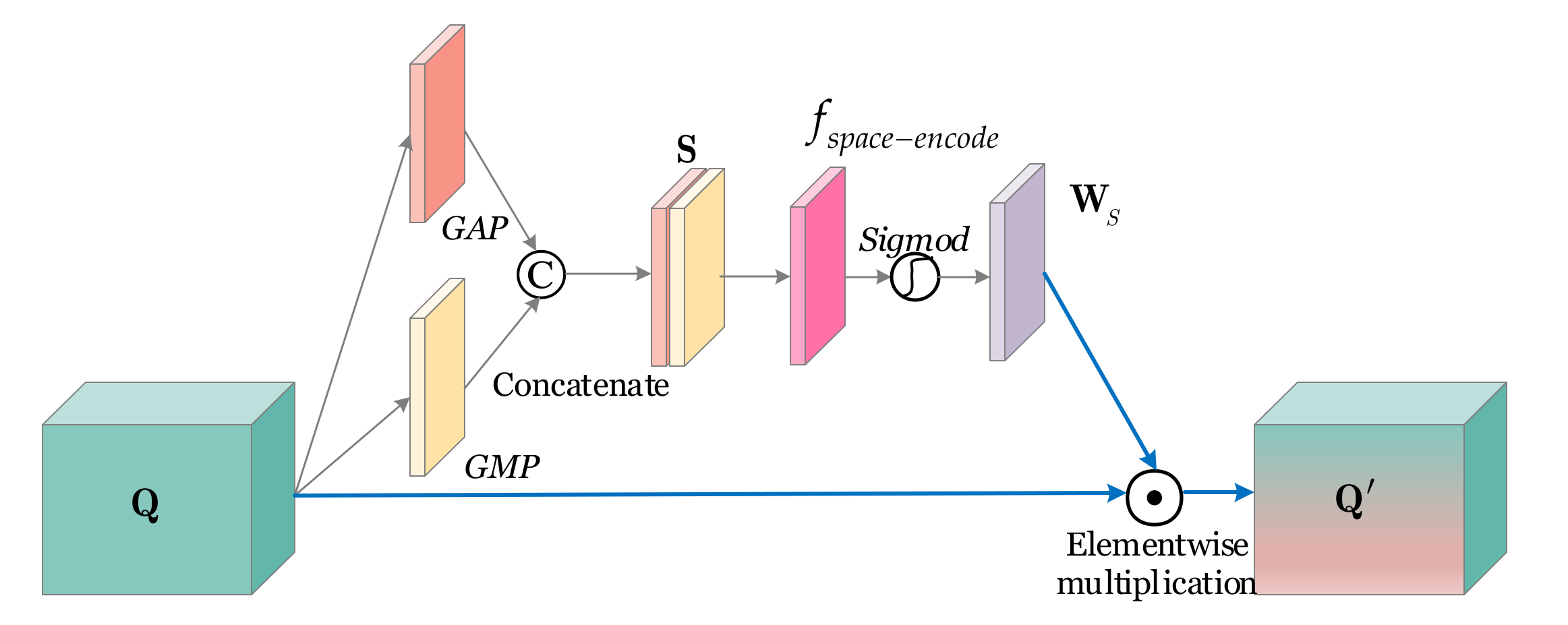
Figure 5 shows the implementation process of PA-SA-Module. In Figure 5, the input feature maps are denoted by Q and the output ones are denoted by Q. First, a global average pooling (GAP) [29] is used to obtain the average response in space; a global max pooling (GMP) [29] is used to obtain the maximum response in space. Then, their implementation results are concatenated as the synthetic feature maps, denoted by S. Unlike the previous convolutional block attention module [28], we design a space encoder fspace-encode to encode the space information. It is used to represent the spatial correlation. This can improve spatial attention gains because features in the coding space are more concentrated. Then, the output of fspace-encode is activated by a sigmod function to represent each pixel’s importance-level in the original space, i.e., an importance-level weight matrix WS. Finally, an elementwise multiplication is conducted between the original feature maps Q and the importance-level weight matrix WS to obtain the output Q.
In short, the above can be described by
Q = Q W S
where Q denotes the input feature maps, Q denotes the output feature maps, ⊙ denotes the elementwise multiplication, and WS denotes the importance-level weight matrix, i.e.,
W S = s i g m o d f s p a c e e n c o d e G A P ( Q ) © G M P ( Q )
where GAP denotes the global average-pooling, GMP denotes the global max-pooling, fspace-encode denotes the space encoder, © denotes the concatenation operation, and sigmod is an activation function defined by 1/(1 + ex).
Finally, the feature pyramid will be stronger when possessing both the top-to-bottom branch and bottom-to-top branch. Each level has rich spatial location information and abundant semantic information, which help improve large ships’ detection performance.

2.4. Balance Scale Global Attention FPN (BS-GA-FPN)

The core idea of BS-GA-FPN is that we further refine features from each feature level in the pyramid, to address the feature level imbalance of different scale ships. SAR ships often present different characteristics at different levels in the pyramid, i.e., the existence of multi-scale ship feature differences. Due to the difference of resolutions, the difference of satellite shooting distances, and different slicing methods, there are many scales of ships in the existing SAR ship datasets. E.g., for SSDD, the smallest ship pixel size is 7 × 7 while the biggest one is 211 × 298. Such huge size gap results in large ship feature differences, which makes it very difficult to detect them. In the computer vision community, Pang et al. [30] found that such feature level imbalance may weaken the feature expression capacity of FPN, but previous work [5,6,7,8,9,10,11,12,13,14,
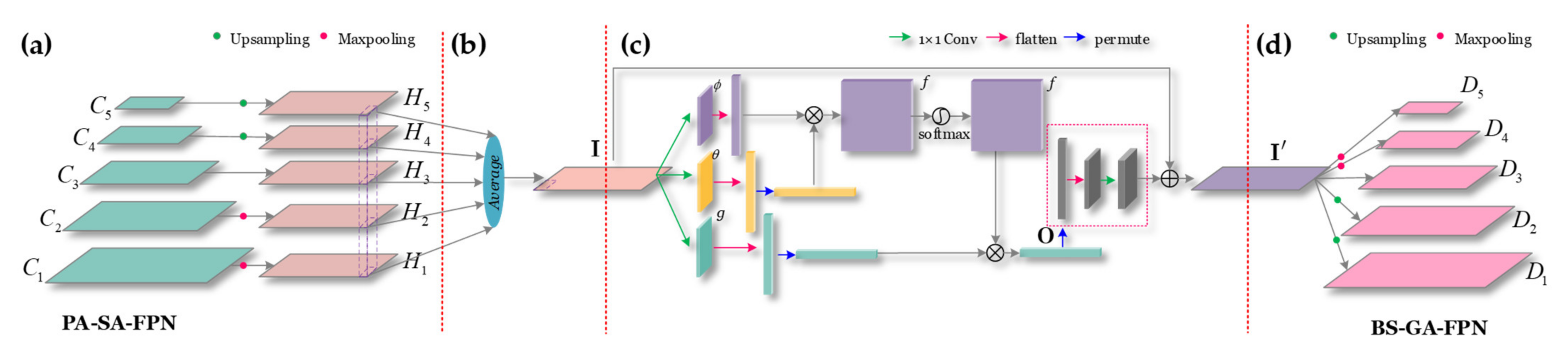
15] in the SAR ship detection community was not aware of this problem. Thus, to handle this problem, we design a BS-GA-Module to further process pyramid features to recover a balanced BS-GA-FPN. Implementation process of BS-GA-Module consists of four steps: (1) feature pyramid resizing, (2) balanced multi-scale feature fusion, (3) global attention (GA) refinement, and (4) feature pyramid recovery, as in Figure 6.
Step 1: Feature Pyramid Resizing
Figure 6a shows the graphical description of the feature pyramid resizing. In Figure 6a, in the PA-SA-FPN, features maps at different levels are denoted by C1, C2, C3, C4, and C5. To facilitate the fusion of balanced features to preserve their semantic hierarchy at the same time, we resize each detection scale (C1, C2, C3, C4, and C5) to a unified resolution, by a max-pooling or up-sampling. Here, C3 is selected as this unified resolution level because it locates in the middle of the pyramid. It can maintain a trade-off between top semantic information and bottom spatial information. Finally, the above can be described by
H 1 = M a x P o o l 4 × ( C 1 ) ,   H 2 = M a x P o o l 2 × ( C 2 ) ,   H 3 = C 3 ,   H 4 = U p S a m p l i n g 2 × ( C 4 ) ,   H 5 = U p S a m p l i n g 4 × ( C 5 )
where H1, H2, H3, H4, and H5 are the resized feature maps from the original ones, UpSamplingn× denotes the n times up-sampling, and MaxPooln× denotes the n times max-pooling.
Step 2: Balanced Multi-Scale Feature Fusion
Figure 6b shows the graphical description of the balanced multi-scale feature fusion. After obtaining feature maps with the same unified resolution, the balanced multi-scale feature fusion is executed by
I ( i , j ) = 1 5 k = 1 5 H k ( i , j )
where k denotes the k-th detection level, (i, j) denotes the spatial location of feature maps, and I denotes the output integrated features. From Equation (11), the features from each scale (H1, H2, H3, H4, and H5) are uniformly fused as the output I (a mean operation). Here, the average operation fully reflects the balanced idea of SAR ship scale feature fusion.
Finally, the output I with condensed multi-scale information will contain balanced semantic features of various resolutions. In this way, big ship features and small ones can complement each other to facilitate the information flow.
Step 3: GA Refinement
To make features from different scales become more discriminative, we also propose a GA refinement mechanism to further refine balanced features in Equation (11). This can enhance their global response ability. That is, the network will pay more attention to important spatial global information (feature self-attention), as in Figure 6c.
The GA refinement can be described by
O i = 1 ξ I × j f I i , I j × g I j
where Ii denotes the input at the i-th location, Oi denotes the output at the i-th location, f(·) is a function used to calculate the similarity between the location Ii and Ij, g(·) is a function to characterize the feature representation at the j-th location, and ξ(·) denotes a normalized coefficient (the input overall response). The i-th location information denotes the current location’s response, and the j-th location information denotes the global response.
In Equation (12), g(·) can be regarded as a linear embedding,
g I j = W g I j
where Wg is a weight matrix to be learned, and we use a 1 × 1 convolutional layer to obtain this weight matrix during training.
Furthermore, one simple extension of the Gaussian function is to compute similarity f(·) in an embedding space,
f ( I i , I j ) = e θ I i T ϕ I j
where θ(Ii) = WθIi and ϕ(Ij) = WϕIj are two embeddings. Wθ and Wϕ are the weight matrixes to be learned that are both achieved by other two 1 × 1 convolutional layers.
As above, the normalized coefficient ξ(·) is set to
ξ I = j f ( I i , I j )
Finally, the whole GA refinement is instantiated as:
O i = e θ I i T ϕ I j × W g I j / j e θ I i T ϕ I j
where e θ I i T ϕ I j / j e θ I i T ϕ I j can be achieved by a soft-max function.
Figure 6c shows the graphical description of the above GA refinement. From Figure 6c, two 1 × 1 convolutional layers are used to compute ϕ and θ. Then, by the matrix multiplication θTϕ, the similarity f is obtained. One 1 × 1 convolutional layer is used to characterize the representation of the features g. Finally, f with a soft-max function multiplies by g to obtain the feature self-attention output O = {Oi | i in I}. Finally, the feature self-attention output O is further processed by one 1 × 1 convolutional layer (marked in a dotted box). The purpose is to make O match the dimension of the original input I to facilitate follow-up element-wise adding. This is similar to the residual/skip connections of ResNet. Consequently, the refined features I′ combining the feature self-attention information are achieved, which will be further processed in the subsequent steps, i.e.,
I = W O O + I
where WO is also a weight matrix to be learned, and another 1 × 1 convolutional layer can be used to obtain it during training.
In essence, the GA refinement can directly capture long-range dependence of each location (global response) by calculating the interaction between two different arbitrary positions. It is equivalent to constructing a convolutional kernel with the same size as the feature map I, to maintain more useful ship information, making feature maps more discriminative. More detailed theories about this global attention can be found in [31].
Step 4: Feature Pyramid Recovery
Figure 6d shows the graphical description of the feature pyramid recovery. From Figure 6d, the refined features I′ are resized again through using the similar but reverse procedure of Equation (10) to recover a balanced feature pyramid, i.e.,
D 1 = U p S a m p l i n g 4 × ( I ) ,   D 2 = U p S a m p l i n g 2 × ( I ) ,   D 3 = I ,   D 4 = M a x P o o l 2 × ( I ) ,   D 5 = M a x P o o l 4 × ( I )
where D1, D2, D3, D4, and D5 denote the recovered feature maps at different levels after ship scale balance operations. They reconstruct the final network architecture of BS-GA-FPN. Ultimately, D1, D2, D3, D4, and D5 in BS-GA-FPN will possess more multi-scale balanced features that will be used to be responsible for the final ship detection.

3. Experiments

Our experiments are run on a personal computer with i9-9900K CPU and RTX2080Ti GPU based on Pytorch. Quad-FPN and the other 12 competitive SAR ship detectors are implemented under the MMDetection toolbox [32] to ensure the comparison fairness.

3.1. Experimental Datasets

(1)
SSDD: SSDD is the first open SAR ship detection dataset, proposed by Li et al. [5] in 2017. There are 1160 SAR images with 500 × 500 average image size in SSDD from Sentinel-1, TerraSAR-X, and RadarSat-2. SAR ships in SSDD are provided with various resolutions from 1m to 10m, and HH, HV, VV, and VH polarizations. We set the ratio of the training set and the test set to 8:2. Here, image names with the index suffix of 1 and 9 are selected as the test set, and the others as the training set.
(2)
Gaofen-SSDD: Gaofen-SSDD was constituted in [6] to make up for the shortcoming of insufficient samples in SSDD. There are 20,000 images with 160 × 160 image size in Gaofen-SSDD from Gaofen-3. SAR ships in Gaofen-SSDD are provided with various resolutions from 5 m to 10 m, and HH, HV, VV, and VH polarizations. Same as [6], the ratio of the training set, validation set, and the test set is 7:2:1 by a random selection.
(3)
Sentinel-SSDD: Sentinel-SSDD was constituted in [6] to make up for the shortcoming of insufficient sample number in SSDD. There are 20,000 images with 160 × 160 image size in Sentinel-SSDD from Sentinel-1. SAR ships in Sentinel-SSDD are provided with resolutions from 5 m to 20 m, and HH, HV, VV, and VH polarizations. Same as [6], the ratio of the training set, validation set, and the test set is 7:2:1 by a random selection.
(4)
SAR-Ship-Dataset: SAR-Ship-Dataset was released by Wang et al. [7] in 2019. There are 43,819 images with 256 × 256 image size in SAR-Ship-Dataset from Sentinel-1 and Gaofen-3. SAR ships in Sentinel-SSDD are provided with resolutions from 5 m to 20 m, and HH, HV, VV, and VH polarizations. Same as their original reports in [7], the ratio of the training set, validation set, and the test set is 7:2:1 by a random selection.
(5)
HRSID: HRSID was released by Wei et al. [8] in 2020. There are 5604 images with 800 × 800 image size in HRSID from Sentinel-1 and TerraSAR-X. SAR ships in HRSID are provided with resolutions from 0.1 m to 3 m, and HH, HV, and VV polarizations. Same as its original reports in [8], the ratio of the training set and the test set is 13:7 according to its default configuration files.

3.2. Experimental Details

ResNet-50 with pretraining on ImageNet [33] serves as Quad-FPNs’ backbone network. Images in SSDD, Gaofen-SSDD, Sentinel-SSDD, SAR-Ship-Dataset, and HRSID are resized as the 512 × 512, 160 × 160, 160 × 160, 256 × 256, and 800 × 800 image size for training. We train Quad-FPN for 12 epochs with a batch size of 2, due to the limited GPU memory. Stochastic gradient descent (SGD) [34] serves as the optimizer with a 0.1 learning rate, a 0.9 momentum, and a 0.0001 weight decay. Moreover, the learning rate is reduced by 10 times per epoch from 8-epoch to 11-epoch to ensure an adequate loss reduction. Followed by Wei et al. [12], a soft non-maximum suppression (Soft-NMS) [35] algorithm is used to suppress duplicate detections with an intersection over union (IOU) threshold of 0.5.

3.3. Loss Function

Followed by Cui et al. [13], the cross entropy (CE) serves as the classification loss Lcls,
L c l s = 1 N i = 1 N p i log ( p i * ) + ( 1 p i ) log ( 1 p i * )
where pi denotes the predictive class probability, pi* denotes the ground truth class label, and N denotes the prediction number. The smoothL1 serves as the regression loss Lreg,
L r e g = 1 N i = 1 N p i * smooth L 1 ( t i t i * ) , w h e r e   smooth L 1 ( x ) = 0.5 x 2   i f   | x | < 1 | x | 0.5   o t h e r w i s e
where ti denotes the predictive bounding box and ti* denotes the ground truth box.

3.4. Evaluation Indices

Evaluation indices from the PASCAL dataset [5] are adopted by this paper, including the recall (r), precision (p), and mean average precision (mAP) [36], i.e.,
r = T P / ( T P + F N ) ,   p = T P / ( T P + F P ) ,   mAP = 0 1 p r × d r
where TP denotes the number of true positives, FN denotes that of false negatives, FP denotes that of false positives, and p(r) denotes the precision-recall curve. In this paper, mAP measures the final detection accuracy because it considers both precision and recall.
Moreover, the frames per second (FPS) is used to measure the detection speed, which is defined by 1/t, where t refers to the time to detect an image, whose unit is the second (s).

4. Results

4.1. Quantitative Results on Five Datasets

Table 1, Table 2, Table 3, Table 4 and Table 5 show the quantitative comparison with the other 12 competitive state-of-the-art CNN-based SAR ship detectors, on SSDD, Gaofen-SSDD, Sentinel-SSDD, SAR-Ship-Dataset, and HRSID. From Table 1, Table 2, Table 3, Table 4 and Table 5, one can clearly find that:
  • On SSDD, Quad-FPN offers the best accuracy (95.29% mAP on the entire scenes). The second-best one is 92.27% mAP in the entire scenes from DCN [24], but it is still lower than Quad-FPN by ~3% mAP, showing the best detection performance of Quad-FPN.
  • On Gaofen-SSDD, Quad-FPN offers the best accuracy (92.84% mAP on the entire scenes). The second-best one is 91.35% mAP in the entire scenes from Free-Anchor, but it is still lower than Quad-FPN by ~1.5% mAP, showing the best detection performance of Quad-FPN.
  • On Sentinel-SSDD, Quad-FPN offers the best accuracy (95.20% mAP on the entire scenes). The second-best one is 94.31% mAP in the entire scenes from Free-Anchor, but it is still lower than Quad-FPN by ~1% mAP, showing the best detection performance of Quad-FPN.
  • On SAR-Ship-Dataset, Quad-FPN offers the best accuracy (94.39% mAP on the entire scenes). The second-best one is 93.70% mAP in the entire scenes from Free-Anchor, but it is still lower than Quad-FPN by ~1% mAP, showing the best detection performance of Quad-FPN.
  • On HRSID, Quad-FPN offers the best detection accuracy (86.12% mAP on the entire scenes). The second-best one is 83.72% mAP in the entire scenes from Guided Anchoring, but it is still lower than Quad-FPN by ~3.5% mAP.
  • Furthermore, for Quad-FPN and the other 12 methods, the detection accuracies of inshore scenes are all lower than that of offshore scenes. This is in line with common sense because the former has more complex backgrounds than the latter.
  • For the more complex inshore scenes, the detection accuracy advantage of Quad-FPN is more obvious than the other 12 methods. Specifically, Quad-FPN offers an accuracy of 84.68% mAP on the SSDD’s inshore scenes, superior to the second-best DCN [24] by ~10% mAP; it offers an accuracy of 85.68% mAP on the Gaofen-SSDD’s inshore scenes, superior to the second-best Free-Anchor by ~4% mAP; it offers an accuracy of 84.68% mAP on the Sentinel-SSDD’s inshore scenes, superior to the second-best Free-Anchor by ~5% mAP; it offers an accuracy of 83.93% mAP on the SAR-Ship-Dataset’s inshore scenes, superior to the second-best Double-Head R-CNN by ~2% mAP; and it offers an accuracy of 70.80% mAP on the HRSID’s inshore scenes, superior to the second-best Guided Anchoring by ~7% mAP. Thus, Quad-FPN seems to be robust for background interferences because the deformable convolution can suppress the interference of complex backgrounds, especially for inshore scenes.
  • The r values of the other 12 methods are lower than Quad-FPN, perhaps from their poor small ship detection performance. The p values of Quad-FPN are sometimes lower than others. Thus, an appropriate score threshold can be further considered in the future to make a trade-off between missed detections and false alarms.
  • To be honest, Quad-FPN sacrifices speed due to the network’s high-complexity. Yet, it is also important to further improve the accuracy, e.g., the precision strike of military targets. In the future, we will make a trade-off between accuracy and speed.

4.2. Qualitative Results on Five Datasets

Figure 7, Figure 8, Figure 9, Figure 10 and Figure 11 show the qualitative results on SSDD, Gaofen-SSDD, Sentinel-SSDD, SAR-Ship-Dataset, and HRSID. Here, we only compare Quad-FPN with the second-best detector, due to limited pages.
Taking SSDD in Figure 7 as an example, we can draw the following conclusions:
  • Quad-FPN can successfully detect various SAR ships with different sizes under various backgrounds. This shows its excellent detection performance with excellent scale-adaptation and scene-adaptation. Compared with the second-best CNN-based ship detector DCN [24], Quad-FPN can improve the detection confidence scores. For example, in the first detection sample of Figure 7, Quad-FPN increases the confidence score from 0.96 to 1.0. This can show Quad-FPN’s higher credibility.
  • Quad-FPN can suppress some false alarms from complex inshore facilities. For example, in the second detection sample of Figure 7, one land false alarm is removed by Quad-FPN. This shows Quad-FPN’s better scene-adaptability.
  • Quad-FPN can avoid some missed detections of densely arranged ships and small ships. For example, in the second sample of Figure 7, small ships densely parked at ports are detected again by Quad-FPN. This is because the adopted deformable convolution in DE-CO-FPN can alleviate the negative influence from the hull of a nearby ship. In the fourth sample of Figure 7, many small ships are detected successfully again by Quad-FPN, but DCN failed most of them. This is because CA-FR-FPN can transmit more abundant semantic information from the pyramid top to the bottom, to improve the expression capacity of small ship features. This shows Quad-FPN’s better detection capacity of both inshore ships and small ones.
  • Moreover, from the third sample of Figure 7, ships with different scales on the same SAR image are detected at the same time. This is because the proposed BS-GA-GPN can balance the feature differences of different sizes of ships, showing Quad-FPN’s excellent scale-adaptability.
Moreover, from the detection results of the second sample on Gaofen-SSDD in Figure 8, Quad-FPN can remove false alarms from ship-like man-made facilities, meanwhile successfully detecting the ship moored at port, even under the strong speckle noise interference, or rather low signal to noise ratio (SNR). This shows Quad-FPN has both keen judgment merits and robust anti-noise performance. Similarly, the detection results of the first three samples on SAR-Ship-Dataset in Figure 10 can also reveal its excellent anti-noise performance. Finally, from the detection results of the third sample on SAR-Ship-Dataset in Figure 10, a large ship parking at port is detected by Quad-FPN again. This is because PA-SA-FPN can transmit the low-level location information from the pyramid bottom to the pyramid top, which can bring more accurate positionings of large ship bounding boxes. Correspondingly, the feature learning benefits of large ships are enhanced, thereby avoiding their missed detections. Given the above, Quad-FPN offers state-of-the-art SAR ship detection performance.

4.3. Large-Scene Application in Sentinel-1 SAR Images

We conduct the actual ship detection in another two large-scene Sentinel-1 SAR images to confirm the good migration capability of Quad-FPN. Figure 12 shows the coverage areas of the two large-scene Sentinel-1 SAR images. The two areas are both the world’s major shipping routes, so they are selected. Table 6 shows their descriptions. From Table 6, the VV polarization SAR images are selected given that ships generally exhibit higher backscattering values in VV polarization [42]. In addition, the interferometric wide-swath (IW) mode of Sentinel-1 is selected specifically because it is the main mode to acquire data in areas of maritime surveillance interest [42]. The ship ground truths are annotated by SAR experts using the automatic identification system (AIS) and Google Earth. This can provide a more reliable performance evaluation. These two SAR images are resized as 24,000 × 16,000 image size, respectively. Then, followed by [43], they are cut into 800 × 800 small sub-images directly for training and testing because of the limited GPU memory. Finally, they are inputted into Quad-FPN for the actual SAR ship detection. After that, the detection results of these sub-images are integrated to the original large-scene SAR image.
Figure 13 shows the visualization SAR ship detection results of Quad-FPN on the two large-scene SAR images. From Figure 13, most ships can be detected by Quad-FPN successfully, which shows its good migration application capability in ocean surveillance.

4.3.1. Quantitative Comparison with State-of-The-Art

Table 7 and Table 8 show their quantitative comparison with the other 12 competitive CNN-based SAR ship detectors. To be clear, in Table 7 and Table 8, the GPU time is selected to compare their speed (tGPU) because modern CNN-based detectors are always run on GPUs. From Table 7 and Table 8, one can find that Quad-FPN achieves the best detection accuracy on the two large-scene SAR images, showing its good migration capability.
On the Image 1, Quad-FPN offers an accuracy of 83.96% mAP, superior to the second-best PANET [37] (83.96% mAP > 80.51% mAP); on the Image 2, Quad-FPN offers an accuracy of 87.03% mAP, superior to the second-best PANET [37] (87.03% mAP > 84.33% mAP). To be honest, we find that Quad-FPN’s detection speed is relatively modest in contrast to others; thus, further detection speed improvements can be performed in the future.

4.3.2. Quantitative Comparison with CFAR

Finally, we perform an experiment to compare performance with a classical and common-used two-parameter CFAR detector. Following the standard implementation process from Deng et al. [44], we obtain the CFAR’s detection results in the Sentinel-1 toolbox [45]. Table 9 and Table 10 show their quantitative detection results.
In Table 9 and Table 10, the traditional CFAR usually does not use mAP from the DL community to measure accuracy, so F1 is used to represent accuracy, defined by:
F 1 = 2 × p × r p + r
Moreover, in Table 9 and Table 10, CFARs are usually run on CPUs, whereas modern DL-based methods are always run on GPUs; to ensure a reasonable comparison, the CPU time is selected for their speed comparison (tCPU). From Table 9 and Table 10, Quad-FPN is greatly superior to CFAR in terms of the detection accuracy, i.e., 0.74 F1 of CFAR on Image 1 << 0.84 F1 of Quad-FPN on Image 1, and 0.69 F1 of CFAR on Image 2 << 0.84 F1 of Quad-FPN on Image 2. The detection speed of Quad-FPN is also greatly superior to CFAR, i.e., 223.15 s CPU time of Quad-FPN on Image 1 << 884.00 s CPU time of CFAR on Image 1, and 226.08 s CPU time of Quad-FPN on Image 2 << 735.00 s CPU time of CFAR on Image 2. Therefore, Quad-FPN might still meet the needs of practical applications.

5. Ablation Study

In this section, ablation studies are conducted to verify the effectiveness of each FPN. We also discuss the advantages of each innovation. Here, we take the SSDD dataset as an example to show the results, due to limited pages. Table 11 shows the effectiveness of the Quad-FPN pipeline (DE-CO-FPN→CA-FR-FPN→PA-SA-FPN→BS-GA-FPN). From Table 11, the detection accuracy is improved step by step from left to right in the Quad-FPN pipeline architecture (89.92% mAP→93.61% mAP→94.58% mAP→95.29% mAP). This can show each FPN’s effectiveness from the perspective of the overall structure.
To be clear, the sequence of the four FPNs is better kept unchanged; otherwise, the final accuracy cannot reach the best level according to our experiments. Some detailed analysis can be found in Section 2 (i.e., the overall design idea of Quad-FPN).

5.1. Ablation Study on DE-CO-FPN

We make two experiments with respect to DE-CO-FPN. Experiment 1 in Section 5.1.1 is used to confirm the effectiveness of DE-CO-FPN, directly. Experiment 2 in Section 5.1.2 is used to confirm the advantage of the deformable convolution.

5.1.1. Experiment 1: Effectiveness of DE-CO-FPN

Table 12 shows the ablation study results on DE-CO-FPM. In Table 12, “” denotes removing DE-CO-FPN (the other three FPNs are reserved) and “” denotes using DE-CO-FPN. From Table 12, DE-CO-FPN improves the accuracy by ~3% mAP, which shows its effectiveness. Combined with it, SAR ship features extracted by networks will contain useful shape information; moreover, they can alleviate complex background interferences.

5.1.2. Experiment 2: Different Types of Convolutions

Table 13 shows the ablation study results on different convolution types. In Table 13, “Standard” denotes the traditional regular convolution in Figure 3a, “Dilated” denotes the dilated convolution in Figure 3b, and “Deformable” denotes the deformable convolution in Figure 3c. From Table 13, the deformable convolution achieves the best detection accuracy because it can more effectively model various ships’ shapes by its adaptive kernel offset learning. This adaptive kernel offset learning can extract the shape and edge features of ships accurately, to suppress the interference of complex backgrounds, especially for the complex inshore scenes. In this way, ships can be separated successfully from complex backgrounds. Thus, this deformable convolution process can be regarded as an extraction of salient objects in various scenes, which plays a role of spatial attention. Accordingly, the accuracy on the overall dataset is improved.

5.2. Ablation Study on CA-FR-FPN

With respect to CA-FR-FPN, we will make two experiments. Experiment 1 in Section 5.2.1 is used to confirm the effectiveness of CA-FR-FPN, directly. Experiment 2 in Section 5.2.2 is used to determine the appropriate feature amplification factor α in CA-FR-Module.

5.2.1. Experiment 1: Effectiveness of CA-FR-FPN

Table 14 shows the ablation study results on CA-FR-FPN. In Table 14, “” denotes removing CA-FR-FPN (i.e., not using the CA-FR-Module, but the other three FPNs are reserved.); “” denotes using the CA-FR-FPN. From Table 14, CA-FR-FPN improves the detection accuracy by ~1% mAP because it can be aware of more valuable information for feature up-sampling. Its adaptive content-aware kernel can improve the transmission benefits of information flow, to improve the detection performance. This is because it can effectively capture the rich semantic information required by dense detection tasks, especially for densely distributed small ships. This can avoid the feature loss because of small ship features’ poor conspicuousness. Accordingly, the accuracy on the overall dataset is improved.

5.2.2. Experiment 2: Different Feature Amplification Factors

Table 15 shows the ablation study results on feature amplification factor α in CA-FR-Module. In Table 15, “” denotes not amplifying features. From Table 15, when features are amplified no matter what the value of α is, the detection accuracy can obtain improvements, compared with not amplifying features. Therefore, the feature amplification can indeed enhance the content-aware benefits of the kernel prediction, no matter what the value of α is. This is because in the embedded feature amplification space, the amount of information of feature maps will be effectively increased, promoting the better correctness of the kernel prediction. Finally, in our Quad-FPN, to obtain a better detection accuracy (95.29% mAP), α is set to an optimal or saturated value 8.

5.3. Ablation Study on PA-SA-FPN

We make three experiments with respect to PA-SA-FPN. Experiment 1 in Section 5.3.1 is used to confirm the effectiveness of PA-SA-FPN, directly. Experiment 2 in Section 5.3.2 is used to confirm the effectiveness of PA-SA-Module. Experiment 3 in Section 5.3.3 is used to confirm the advantage of PA-SA-Module.

5.3.1. Experiment 1: Effectiveness of PA-SA-FPN

Table 16 shows the ablation study results on PA-SA-FPN. In Table 16, “” denotes removing PA-SA-FPN (the other three FPNs are reserved); “” denotes using PA-SA-FPN. From Table 16, PA-SA-FPN improves the detection accuracy by ~1.5% mAP because the low-level spatial location information in the pyramid bottom has been transmitted to the top in PA-SA-FPN. In this way, the positionings of large ship bounding boxes will become more accurate. Accordingly, the accuracy on the overall dataset is improved.

5.3.2. Experiment 2: Effectiveness of PA-SA-Module

Table 17 shows the ablation study results on PA-SA-Module. From Table 17, PA-SA-Module can effectively enhance the detection accuracy by ~1% mAP because it can enable more pivotal spatial information in the pyramid bottom be effectively transmitted to the top. This can improve path aggregation benefits. In this way, the features of large ships might become richer and more discriminative. Accordingly, the accuracy on the overall dataset is improved.

5.3.3. Experiment 3: Different Attention Types

Table 18 shows the ablation study results on different attention types. In Table 18, “SE” denotes the squeeze-and-excitation mechanism [36] and “CBAM” denotes the convolutional block attention module [28]. From Table 18, PA-SA-Module is superior to others because it can cause key spatial global information to be transmitted more efficiently, which means that it is more suitable for PA-SA-FPN. Moreover, different from the previous CBAM, our designed space encoder fspace-encode can encode the space information. It is can represent the spatial correlation more effectively. This can improve spatial attention gains because the features in the coding space are more concentrated.

5.4. Ablation Study on BS-GA-FPN

We conduct three experiments with respect to BS-GA-FPN. Experiment 1 in Section 5.4.1 is used to confirm the effectiveness of BS-GA-FPN, directly. Experiment 2 in Section 5.4.2 is used to confirm the effectiveness of GA. Experiment 3 in Section 5.4.3 is used to confirm the advantage of GA.

5.4.1. Experiment 1: Effectiveness of BS-GA-FPN

Table 19 shows the ablation study results on BS-GA-FPN. In Table 19, “” denotes removing BS-GA-FPN (the other three FPNs are reserved); “” denotes using BS-GA-FPN. From Table 19, BS-GA-FPN can play an important role in ensuring higher detection accuracy because it can improve the accuracy by ~1% mAP. In this way, ship multi-scale features can be effectively balanced, which can achieve a stronger feature expression capacity of the final FPN. Accordingly, the accuracy on the overall dataset is improved.

5.4.2. Experiment 2: Effectiveness of GA

Table 20 shows the ablation study results on GA. From Table 20, GA can improve the detection accuracy because when various ship multi-scale features are refined by it, they can become more discriminative. This feature self-attention might amplify important global information and suppress tiresome interferences, which can enhance the feature expressiveness of FPN. Essentially, GA is able to directly capture long-range dependence of each location (global response) through calculating the interaction between two different arbitrary positions. The whole GA refinement is essentially equivalent to construct a convolutional kernel with the same size as the feature map, to maintain more useful ship information. Accordingly, the accuracy on the overall dataset is improved.

5.4.3. Experiment 3: Different Refinement Types

Table 21 shows the ablation study results of different refinement types. In Table 21, we compare three refinement types, including a convolutional layer, an SE [36], and a CBAM [28]. From Table 21, GA offers the best detection accuracy because it can directly capture long-range dependence of each location (global response) to maintain more useful ship information that makes feature maps more discriminative. Different from the traditional convolution refinement types, its receptive field is wider, i.e., the whole input feature map’s size, resulting in a better spatial correlation learning. Accordingly, the accuracy on the overall dataset is improved.

6. Conclusions

Aiming at some challenges in SAR ship detection, e.g., complex background interferences, multi-scale ship feature differences, and indistinctive small ship features, a novel Quad-FPN is proposed for SAR ship detection in this paper. Quad-FPN consists of four unique FPNs that can guarantee its excellent detection performance, i.e., DE-CO-FPN, CA-FR-FPN, PA-SA-FPN, and BS-GA-FPN. In DE-CO-FPN, we adopt the deformable convolution to extract SAR ship features that will contain more useful ship shape information, meanwhile alleviating complex background interferences. In CA-FR-FPN, we design a CA-FR-Module to enhance feature transmission benefits when performing the up-sampling multi-level feature fusion. In PA-SA-FPN, we add an extra path aggregation branch with a space attention module from the pyramid bottom to the top. In BS-GA-FPN, we further refine features from each feature level in the pyramid to address feature level imbalance of different scale ships. We perform extensive ablation studies to confirm the effectiveness of each FPN. Experimental results on five open datasets jointly reveal that Quad-FPN can offer the most superior SAR ship detection performance compared with the other 12 competitive state-of-the-art CNN-based SAR ship detectors. Moreover, the satisfactory detection results in two large-scene Sentinel-1 SAR images showing Quad-FPN’s excellent migration capability in ocean surveillance. Quad-FPN is an excellent two-stage SAR ship detector. Four FPNs’ internal implementations are different from previous work. They are well-designed improvements to ensure the state-of-the-art detection performance, without bells and whistles. They can exactly enable Quad-FPN’s excellent ship scale-adaptability and detection scene-adaptability.
Our future work is as follows:
  • We will consider the cost of deformable convolutions, in the future.
  • We will consider optimizing the detection speed of Quad-FPN, in the future.
  • We will further study the effect of four FPNs’ sequence on performance, in the future.
  • We will consider the challenges within SAR data, e.g., the azimuth ambiguity, sidelobes, and the sea state, to optimize Quad-FPN’s detection performance, in the future.
  • We will consider making efforts to combine modern deep CNN abstract features and traditional concrete ones to further improve detection accuracy, in the future.

Author Contributions

Conceptualization, T.Z.; methodology, T.Z.; software, T.Z.; validation, T.Z.; formal analysis, T.Z.; investigation, T.Z.; resources, T.Z.; data curation, T.Z.; writing—original draft preparation, T.Z.; writing—review and editing, X.Z. and X.K.; visualization, T.Z.; supervision, X.Z.; project administration, X.Z.; funding acquisition, X.Z. All authors have read and agreed to the published version of the manuscript.

Funding

This work was supported by the National Natural Science Foundation of China (61571099).

Institutional Review Board Statement

Not applicable.

Informed Consent Statement

Not applicable.

Data Availability Statement

No new data were created or analyzed in this study. Data sharing is not applicable to this article.

Acknowledgments

The authors would like to thank the editors and the four anonymous reviewers for their valuable comments that can greatly improve our manuscript.

Conflicts of Interest

The authors declare no conflict of interest.

References

  1. Liu, T.; Zhang, J.; Gao, G.; Yang, J.; Marino, A. CFAR Ship Detection in Polarimetric Synthetic Aperture Radar Images Based on Whitening Filter. IEEE Trans. Geosci. Remote Sens. 2020, 58, 58–81. [Google Scholar] [CrossRef]
  2. Yang, M.; Guo, C.; Zhong, H.; Yin, H. A Curvature-Based Saliency Method for Ship Detection in SAR Images. IEEE Geosci. Remote Sens. Lett. 2020, 1–5. [Google Scholar] [CrossRef]
  3. Lin, H.; Chen, H.; Jin, K.; Zeng, L.; Yang, J. Ship Detection with Superpixel-Level Fisher Vector in High-Resolution SAR Images. IEEE Geosci. Remote Sens. Lett. 2020, 17, 247–251. [Google Scholar] [CrossRef]
  4. Schwegmann, C.P.; Kleynhans, W.; Salmon, B.P. Synthetic Aperture Radar Ship Detection Using Haar-Like Features. IEEE Geosci. Remote Sens. Lett. 2017, 14, 154–158. [Google Scholar] [CrossRef] [Green Version]
  5. Li, J.; Qu, C.; Shao, J. Ship detection in SAR images based on an improved faster R-CNN. In Proceedings of the SAR in Big Data Era: Models, Methods and Applications, Beijing, China, 13–14 November 2017; pp. 1–6. [Google Scholar]
  6. Zhang, T.; Zhang, X.; Shi, J.; Wei, S. HyperLi-Net: A hyper-light deep learning network for high-accurate and high-speed ship detection from synthetic aperture radar imagery. ISPRS J. Photogramm. Remote Sens. 2020, 167, 123–153. [Google Scholar] [CrossRef]
  7. Wang, Y.; Wang, C.; Zhang, H.; Dong, Y.; Wei, S. A SAR Dataset of Ship Detection for Deep Learning under Complex Backgrounds. Remote Sens. 2019, 11, 765. [Google Scholar] [CrossRef] [Green Version]
  8. Wei, S.; Zeng, X.; Qu, Q.; Wang, M.; Su, H.; Shi, J. HRSID: A High-Resolution SAR Images Dataset for Ship Detection and Instance Segmentation. IEEE Access 2020, 8, 120234–120254. [Google Scholar] [CrossRef]
  9. Li, J.; Qu, C.; Peng, S. A ship detection method based on cascade CNN in SAR images. Control Decis. 2019, 34, 2191–2197. [Google Scholar]
  10. Zhang, T.; Zhang, X.; Shi, J.; Wei, S. Depthwise Separable Convolution Neural Network for High-Speed SAR Ship Detection. Remote Sens. 2019, 11, 2483. [Google Scholar] [CrossRef] [Green Version]
  11. Yang, R.; Wang, G.; Pan, Z.; Lu, H.; Zhang, H.; Jia, X. A Novel False Alarm Suppression Method for CNN-Based SAR Ship Detector. IEEE Geosci. Remote Sens. Lett. 2020, 1–5. [Google Scholar] [CrossRef]
  12. Wei, S.; Su, H.; Ming, J.; Wang, C.; Yan, M.; Kumar, D.; Shi, J.; Zhang, X. Precise and Robust Ship Detection for High-Resolution SAR Imagery Based on HR-SDNet. Remote Sens. 2020, 12, 167. [Google Scholar] [CrossRef] [Green Version]
  13. Cui, Z.; Li, Q.; Cao, Z.; Liu, N. Dense Attention Pyramid Networks for Multi-Scale Ship Detection in SAR Images. IEEE Trans. Geosci. Remote Sens. 2019, 57, 8983–8997. [Google Scholar] [CrossRef]
  14. Lin, Z.; Ji, K.; Leng, X.; Kuang, G. Squeeze and Excitation Rank Faster R-CNN for Ship Detection in SAR Images. IEEE Geosci. Remote Sens. Lett. 2019, 16, 751–755. [Google Scholar] [CrossRef]
  15. Zhao, Y.; Zhao, L.; Xiong, B.; Kuang, G. Attention Receptive Pyramid Network for Ship Detection in SAR Images. IEEE J. Sel. Top. Appl. Earth Obs. Remote Sens. 2020, 13, 2738–2756. [Google Scholar] [CrossRef]
  16. Girshick, R. Fast R-CNN. In Proceedings of the IEEE International Conference on Computer Vision (ICCV), Santiago, Chile, 7–13 December 2015; pp. 1440–1448. [Google Scholar]
  17. Ren, S.; He, K.; Girshick, R.; Sun, J. Faster R-CNN: Towards Real-Time Object Detection with Region Proposal Networks. IEEE Trans. Pattern Anal. Mach. Intell. 2017, 39, 1137–1149. [Google Scholar] [CrossRef] [Green Version]
  18. Redmon, J.; Farhadi, A. YOLOv3: An Incremental Improvement. arXiv 2018, arXiv:1804.02767. [Google Scholar]
  19. Lin, T.-Y.; Goyal, P.; Girshick, R.; He, K.; Dollar, P. Focal Loss for Dense Object Detection. IEEE Trans. Pattern Anal. Mach. Intell. 2020, 42, 318–327. [Google Scholar] [CrossRef] [Green Version]
  20. Liu, W.; Anguelov, D.; Erhan, D.; Szegedy, C.; Reed, S.; Fu, C.-Y.; Berg, A.C. SSD: Single Shot MultiBox Detector. In Proceedings of the European Conference on Computer Vision (ECCV), Amsterdam, The Netherlands, 8–16 October 2016; Springer International Publishing: Cham, Switzerland, 2016; pp. 21–37. [Google Scholar]
  21. Cai, Z.; Vasconcelos, N. Cascade R-CNN: Delving into High Quality Object Detection. In Proceedings of the IEEE/CVF Conference on Computer Vision and Pattern Recognition (CVPR), Salt Lake City, UT, USA, 18–23 June 2018; pp. 6154–6162. [Google Scholar]
  22. Lin, T.-Y.; Dollar, P.; Girshick, R.; He, K.; Hariharan, B.; Belongie, S. Feature Pyramid Networks for Object Detection. In Proceedings of the IEEE Conference on Computer Vision and Pattern Recognition (CVPR), Honolulu, HI, USA, 21–26 July 2017; pp. 936–944. [Google Scholar]
  23. Github. Available online: https://github.com/TianwenZhang0825/Quad-FPN (accessed on 25 June 2021).
  24. Dai, J.; Qi, H.; Xiong, Y.; Li, Y.; Zhang, G.; Hu, H.; Wei, Y. Deformable Convolutional Networks. In Proceedings of the IEEE International Conference on Computer Vision (ICCV), Venice, Italy, 22–29 October 2017; pp. 764–773. [Google Scholar]
  25. Yu, F.; Koltun, V. Multi-scale context aggregation by dilated convolutions. arXiv 2016, arXiv:1511.07122. [Google Scholar]
  26. Wang, J.; Chen, K.; Xu, R.; Liu, Z.; Loy, C.C.; Lin, D. CARAFE: Content-Aware ReAssembly of FEatures. In Proceedings of the IEEE/CVF International Conference on Computer Vision (ICCV), Seoul, Korea, 27 October–2 November 2019; pp. 3007–3016. [Google Scholar]
  27. Shi, W.; Caballero, J.; Huszar, F.; Totz, J.; Aitken, A.P.; Bishop, R.; Rueckert, D.; Wang, Z. Real-Time Single Image and Video Super-Resolution Using an Efficient Sub-Pixel Convolutional Neural Network. In Proceedings of the IEEE Conference on Computer Vision and Pattern Recognition (CVPR), Las Vegas, NV, USA, 27–30 June 2016; pp. 1874–1883. [Google Scholar]
  28. Woo, S.; Park, J.; Lee, J.-Y.; Kweon, I.S. CBAM: Convolutional Block Attention Module. arXiv 2018, arXiv:1807.06521. [Google Scholar]
  29. Lin, M.; Chen, Q.; Yan, S. Network in Network. arXiv 2013, arXiv:1312.4400. [Google Scholar]
  30. Pang, J.; Chen, K.; Shi, J.; Feng, H.; Ouyang, W.; Lin, D. Libra R-CNN: Towards Balanced Learning for Object Detection. arXiv 2019, arXiv:1904.02701. [Google Scholar]
  31. Wang, X.; Girshick, R.; Gupta, A.; He, K. Non-local Neural Networks. arXiv 2017, arXiv:1711.07971. [Google Scholar]
  32. Chen, K.; Wang, J.; Pang, J.; Cao, Y.; Xiong, Y.; Li, X.; Sun, S.; Feng, W.; Liu, Z.; Xu, J.; et al. MMDetection: Open MMLab Detection Toolbox and Benchmark. arXiv 2019, arXiv:1906.07155. [Google Scholar]
  33. He, K.; Girshick, R.; Doll´ar, P. Rethinking ImageNet Pre-Training. arXiv 2019, arXiv:1811.08883. [Google Scholar]
  34. Goyal, P.; Dollár, P.; Girshick, R.; Noordhuis, P.; Wesolowski, L.; Kyrola, A.; Tulloch, A.; Jia, Y.; He, K. Accurate, Large Minibatch SGD: Training ImageNet in 1 Hour. arXiv 2017, arXiv:1706.02677. [Google Scholar]
  35. Bodla, N.; Singh, B.; Chellappa, R.; Davis, L.S. Soft-NMS—Improving Object Detection with One Line of Code. In Proceedings of the IEEE International Conference on Computer Vision (ICCV), Venice, Italy, 22–29 October 2017; pp. 5562–5570. [Google Scholar]
  36. Hu, J.; Shen, L.; Albanie, S.; Sun, G.; Wu, E. Squeeze-and-Excitation Networks. IEEE Trans. Pattern Anal. Mach. Intell. 2020, 42, 2011–2023. [Google Scholar] [CrossRef] [Green Version]
  37. Liu, S.; Qi, L.; Qin, H.; Shi, J.; Jia, J. Path Aggregation Network for Instance Segmentation. In Proceedings of the IEEE/CVF Conference on Computer Vision and Pattern Recognition (CVPR), Salt Lake City, UT, USA, 18–23 June 2018; pp. 8759–8768. [Google Scholar]
  38. Wu, Y.; Chen, Y.; Yuan, L.; Liu, Z.; Wang, L.; Li, H.; Fu, Y. Rethinking Classification and Localization for Object Detection. In Proceedings of the IEEE/CVF Conference on Computer Vision and Pattern Recognition (CVPR), Seattle, DC, USA, 16–18 June 2020; pp. 10183–10192. [Google Scholar]
  39. Lu, X.; Li, B.; Yue, Y.; Li, Q.; Yan, J. Grid R-CNN. In Proceedings of the 2019 IEEE/CVF Conference on Computer Vision and Pattern Recognition (CVPR), Long Beach, CA, USA, 16–20 June 2019; pp. 7355–7364. [Google Scholar]
  40. Wang, J.; Chen, K.; Yang, S.; Loy, C.C.; Lin, D. Region Proposal by Guided Anchoring. In Proceedings of the 2019 IEEE/CVF Conference on Computer Vision and Pattern Recognition (CVPR), Long Beach, CA, USA, 16–20 June 2019; pp. 2960–2969. [Google Scholar]
  41. Zhang, X.; Wan, F.; Liu, C.; Ji, R.; Ye, Q. FreeAnchor: Learning to Match Anchors for Visual Object Detection. In Proceedings of the International Conference on Neural Information Processing Systems (NIPS), Vancouver, CO, Canada, 10–12 December 2019; pp. 147–155. [Google Scholar]
  42. Torres, R.; Snoeij, P.; Geudtner, D.; Bibby, D.; Davidson, M.; Attema, E.; Potin, P.; Rommen, B.; Floury, N.; Brown, M.; et al. GMES Sentinel-1 mission. Remote Sens. Environ. 2012, 120, 9–24. [Google Scholar] [CrossRef]
  43. Zhang, T.; Zhang, X.; Ke, X.; Zhan, X.; Shi, J.; Wei, S.; Pan, D.; Li, J.; Su, H.; Zhou, Y.; et al. LS-SSDD-v1.0: A Deep Learning Dataset Dedicated to Small Ship Detection from Large-Scale Sentinel-1 SAR Images. Remote Sens. 2020, 12, 2997. [Google Scholar] [CrossRef]
  44. Deng, Z.; Sun, H.; Zhou, S.; Zhao, J.; Lei, L.; Zou, H. Multi-scale object detection in remote sensing imagery with convolutional neural networks. ISPRS J. Photogramm. Remote Sens. 2018, 145, 3–22. [Google Scholar] [CrossRef]
  45. Sentinel-1 Toolbox. Available online: https://sentinels.copernicus.eu/web/ (accessed on 4 April 2021).
Figure 1. Pipeline structure of Quad-FPN.
Remotesensing 13 02771 g001
Figure 2. Network architecture of Quad-FPN. (a) DE-CO-FPN; (b) CA-FR-FPN; (c) PA-SA-FPN; and (d) BS-GA-FPN.
Remotesensing 13 02771 g002
Figure 3. Different convolutions. (a) Standard convolution; (b) dilated convolution; and (c) deformable convolution.
Remotesensing 13 02771 g003
Figure 4. Implementation process of CA-FR-Module in CA-FR-FPN. (a) Kernel prediction; (b) content-aware feature reassembly.
Remotesensing 13 02771 g004
Figure 5. Implementation process of PA-SA-Module in PA-SA-FPN.
Remotesensing 13 02771 g005
Figure 6. Implementation process of BS-GA-Module. (a) Feature pyramid resizing; (b) balanced multi-scale feature fusion; (c) GA refinement; and (d) feature pyramid recovery.
Remotesensing 13 02771 g006
Figure 7. SAR ship detection results on SSDD. (a) Ground truths; (b) detection results of the second-best DCN [24]; and (c) detection results of the first-best Quad-FPN. Missed detections are marked by red boxes; false alarms are marked by orange boxes.
Remotesensing 13 02771 g007
Figure 8. SAR ship detection results on Gaofen-SSDD. (a) Ground truth; (b) detection results of the second-best Free-Anchor [41]; and (c) detection results of the first-best Quad-FPN. Missed detections are marked by red boxes; false alarms are marked by orange boxes.
Remotesensing 13 02771 g008
Figure 9. SAR ship detection results on Sentinel-SSDD. (a) Ground truths; (b) detection results of the second-best Free-Anchor [41]; and (c) detection results of the first-best Quad-FPN. Missed detections are marked by red boxes; false alarms are marked by orange boxes.
Remotesensing 13 02771 g009
Figure 10. SAR ship detection results on SAR-Ship-Dataset. (a) Ground truths; (b) detection results of the second-best Free-Anchor [41]; and (c) detection results of the first-best Quad-FPN. Missed detections are marked by red boxes; false alarms are marked in orange.
Remotesensing 13 02771 g010
Figure 11. SAR ship detection results on HRSID. (a) Ground truths; (b) detection results of the second-best Guided Anchoring [40]; and (c) detection results of the first-best Quad-FPN. Missed detections are marked by red boxes; false alarms are marked by orange boxes.
Remotesensing 13 02771 g011
Figure 12. Coverage areas of two large-scene Sentinel-1 SAR images. (a) Singapore Strait; (b) Gulf of Cadiz.
Remotesensing 13 02771 g012
Figure 13. Detection results in two large-scene Sentinel-1 SAR images. (a) Image 1; (b) Image 2. Detections are marked by blue boxes.
Remotesensing 13 02771 g013aRemotesensing 13 02771 g013b
Table 1. Quantitative evaluation indices comparison with the other 12 state-of-the-art CNN-based detectors on SSDD.
No.MethodEntire ScenesInshore ScenesOffshore ScenesFPS
r (%)p (%)mAP (%)r (%)p (%)mAP (%)r (%)p (%)mAP (%)
1Faster R-CNN [22]90.4487.0889.7475.0068.9871.3997.5896.0397.3711.87
2PANET [37]91.9186.8191.1577.3367.1772.9298.6697.0998.4811.65
3Cascade R-CNN [21]90.8194.1090.5074.4284.2172.7598.3998.1298.329.46
4Double-Head R-CNN [38]91.9186.9691.1078.4968.1874.9798.1296.8297.826.52
5Grid R-CNN [39]89.7187.7788.9270.9368.1667.4098.3997.0898.139.18
6DCN [24]93.0186.2092.2779.6564.9374.8699.1998.1499.1211.28
7Guided Anchoring [40]90.4494.6290.0173.2686.9071.5998.3997.6098.229.64
8Free-Anchor [41]92.6572.3191.0480.8145.4272.3798.1293.3597.7212.76
9HR-SDNet [12]90.9996.4990.8274.4290.7873.6598.6698.6698.595.79
10DAPN [13]91.3685.5490.5677.9164.1173.2297.5897.5897.4112.22
11SER Faster R-CNN [14]92.2886.1191.5279.0766.3474.5698.3996.8398.2611.64
12ARPN [15]90.6285.4489.8575.0063.8670.7097.8597.0797.7012.15
13Quad-FPN (Ours)95.7789.5295.2987.7974.7584.6899.4697.3799.3811.37
The best detector is bold and the second-best is underlined.
Table 2. Quantitative evaluation indices comparison with the other 12 state-of-the-art CNN-based detectors on Gaofen-SSDD.
No.MethodEntire ScenesInshore ScenesOffshore ScenesFPS
r (%)p (%)mAP (%)r (%)p (%)mAP (%)r (%)p (%)mAP (%)
1Faster R-CNN [22]86.7188.1384.2579.9777.6373.9989.1592.1987.5621.44
2PANET [37]85.4687.4083.1276.8376.2571.3888.6091.6287.0321.94
3Cascade R-CNN [21]89.0690.9287.1280.7382.5075.8492.0893.9790.8917.40
4Double-Head R-CNN [38]87.2888.4785.0380.2378.0674.8389.8492.4688.389.04
5Grid R-CNN [39]87.1186.7384.5479.8573.7273.0189.7591.9888.2015.27
6DCN [24]87.7886.9185.1680.3575.5074.2990.4891.3688.7219.42
7Guided Anchoring [40]91.4791.7289.9185.1485.1480.8793.7894.1292.8517.98
8Free-Anchor [41]93.3974.7491.3587.7854.6781.1495.4285.2194.3824.49
9HR-SDNet [12]91.0491.5989.4382.6282.8378.1894.1094.7993.167.93
10DAPN [13]88.5587.0186.0980.3575.7774.6291.5391.3289.8821.25
11SER Faster R-CNN [14]85.7087.4083.2777.7176.7471.9388.6091.4586.9720.81
12ARPN [15]91.5490.6289.7378.5176.9076.7390.6492.3892.2321.05
13Quad-FPN (Ours)95.3775.5892.8494.2159.5585.6895.7983.6294.5421.81
The best detector is bold and the second-best is underlined.
Table 3. Quantitative evaluation indices comparison with the other 12 state-of-the-art CNN-based detectors on Sentinel-SSDD.
No.MethodEntire ScenesInshore ScenesOffshore ScenesFPS
r (%)p (%)mAP (%)r (%)p (%)mAP (%)r (%)p (%)mAP (%)
1Faster R-CNN [22]91.6388.3190.6476.7067.8270.1496.8996.4296.5123.07
2PANET [37]92.3488.1691.3878.5767.6471.4797.1996.4996.9122.59
3Cascade R-CNN [21]91.6791.7690.9476.1976.0671.1797.1397.3096.9115.31
4Double-Head R-CNN [38]92.1690.0991.3578.0671.3872.2497.1397.3096.857.76
5Grid R-CNN [39]91.2886.1690.1676.5362.3367.7796.4796.4796.167.59
6DCN [24]92.8387.4491.7980.4465.4272.5597.1996.9596.869.57
7Guided Anchoring [40]92.8793.8392.2080.9583.8076.8197.0797.2496.869.35
8Free-Anchor [41]95.0083.5094.3186.2258.1479.7798.0896.5297.9824.82
9HR-SDNet [12]93.7192.0492.9782.4876.5076.4597.6697.9697.558.32
10DAPN [13]91.5488.6090.5576.3668.0369.9796.8996.7196.5121.24
11SER Faster R-CNN [14]92.0787.7691.0877.8967.1671.3297.0796.0996.7022.80
12ARPN [15]92.6089.0691.4884.6378.7277.6297.6996.8097.1921.10
13Quad-FPN (Ours)96.2884.1395.2092.5261.4084.6897.6096.0097.3022.03
The best detector is bold and the second-best is underlined.
Table 4. Quantitative evaluation indices comparison with the other 12 state-of-the-art CNN-based detectors on SAR-Ship-Dataset.
No.MethodEntire ScenesInshore ScenesOffshore ScenesFPS
r (%)p (%)mAP (%)r (%)p (%)mAP (%)r (%)p (%)mAP (%)
1Faster R-CNN [22]93.2486.8591.7386.8069.5579.4795.3693.8594.6523.74
2PANET [37]93.4486.8992.0187.1570.3780.5795.5293.4894.8123.24
3Cascade R-CNN [21]93.4890.5092.2786.1277.4980.9395.9095.2395.3116.80
4Double-Head R-CNN [38]94.1688.4992.9188.1872.4082.1296.1394.8695.569.06
5Grid R-CNN [39]93.0885.1891.4885.5065.5477.6295.5893.4394.8616.39
6DCN [24]93.2586.2591.8087.0868.1580.2195.2993.7494.6020.62
7Guided Anchoring [40]93.8092.5992.7386.1282.5481.7496.3396.0395.7917.41
8Free-Anchor [41]94.9183.9993.7088.0464.0581.6197.1792.6096.6924.64
9HR-SDNet [12]93.2992.1192.2986.1980.8081.8895.6396.1195.147.88
10DAPN [13]93.3487.2891.9786.9470.0880.3495.4594.2194.8121.53
11SER Faster R-CNN [14]93.5886.7892.1887.0169.3780.2495.7493.8395.1122.84
12ARPN [15]92.0188.1191.3587.9272.7781.1495.0094.7995.1021.52
13Quad-FPN (Ours)96.1077.5594.3992.3755.0183.9397.3388.9596.5922.96
The best detector is bold and the second-best is underlined.
Table 5. Quantitative evaluation indices comparison with the other 12 state-of-the-art CNN-based detectors on HRSID.
No.MethodEntire ScenesInshore ScenesOffshore ScenesFPS
r (%)p (%)mAP (%)r (%)p (%)mAP (%)r (%)p (%)mAP (%)
1Faster R-CNN [22]81.9781.4580.6665.5165.5560.1097.1795.9397.0914.05
2PANET [37]82.9881.2881.5967.5565.8361.7597.2495.6897.1413.00
3Cascade R-CNN [21]82.2487.1481.2766.0374.5061.9397.2197.5297.1411.14
4Double-Head R-CNN [38]83.3681.7382.0968.3666.3763.1497.2196.1797.137.05
5Grid R-CNN [39]80.9182.8279.4263.6066.8557.2596.8896.8596.7811.07
6DCN [24]83.4781.4682.0968.3265.8262.3997.4796.2897.3912.66
7Guided Anchoring [40]84.6290.4183.7270.6481.2266.9997.5397.8297.4610.49
8Free-Anchor [41]84.3965.7581.8470.0545.0160.0197.6394.6197.5315.76
9HR-SDNet [12]82.3488.8981.5265.9677.6962.4597.4797.6997.416.74
10DAPN [13]83.3780.5081.8468.5064.7862.2997.1195.6297.0112.93
11SER Faster R-CNN [14]82.9780.0581.5167.4163.6261.4197.3495.8797.2313.59
12ARPN [15]83.8385.7481.7668.1170.7463.5297.0497.2797.3512.80
13Quad-FPN (Ours)87.2987.9686.1275.7877.3170.8097.9297.5797.8613.35
The best detector is bold and the second-best is underlined.
Table 6. Descriptions of two large-scene Sentinel-1 SAR images.
No.PlaceTimePolarizationModeResolution (Range × Azimuth)Image Size
Image 1Singapore Strait6 June 2020VVIW5 m × 20 m25,650 × 16,786
Image 2Gulf of Cadiz18 June 2020VVIW5 m × 20 m25,644 × 16,722
Table 7. Quantitative evaluation indices comparison with the 12 state-of-the-art CNN-based SAR ship detectors on Image 1.
No.MethodGTDetectionsTPFPFNr (%)p (%)mAP (%)tGPU (s)
1Faster R-CNN [22]7607076198814181.4587.5579.4371.93
2PANET [37]7607256309513082.8986.9080.5176.33
3Cascade R-CNN [21]7605084882027264.2196.0663.4183.13
4Double-Head R-CNN [38]7607136219213981.7187.1079.53113.40
5Grid R-CNN [39]76078063714312383.8281.6780.3676.76
6DCN [24]7607156189714281.3286.4379.3374.36
7Guided Anchoring [40]7604514341732657.1196.2355.93102.20
8Free-Anchor [41]760118765153610985.6654.8479.5567.09
9HR-SDNet [12]7605094901927064.4796.2763.78110.83
10DAPN [13]7607076169114481.0587.1378.7676.61
11SER Faster R-CNN [14]7606785997916178.8288.3577.2870.53
12ARPN [15]7607126209215480.1087.0878.9875.14
13Quad-FPN (Ours)7609046622429887.1173.2383.96122.97
The best detector is bold and the second-best is underlined.
Table 8. Quantitative evaluation indices comparison with the 12 state-of-the-art CNN-based SAR ship detectors on Image 2.
No.MethodGTDetectionsTPFPFNr (%)p (%)mAP (%)tGPU (s)
1Faster R-CNN [22]351324290346182.6289.5181.7670.27
2PANET [37]351337299385285.1988.7284.3374.93
3Cascade R-CNN [21]35126025559672.6598.0872.4681.74
4Double-Head R-CNN [38]351336298385384.9088.6984.32112.53
5Grid R-CNN [39]351392296965584.3375.5182.7074.33
6DCN [24]351334291436082.9187.1381.5273.00
7Guided Anchoring [40]351222219313262.3998.6562.21101.37
8Free-Anchor [41]3515863022844986.0451.5481.2167.00
9HR-SDNet [12]35126425689572.9396.9772.51106.88
10DAPN [13]351335292435983.1987.1682.3875.25
11SER Faster R-CNN [14]351323291326082.9190.0981.9470.56
12ARPN [15]351348298506282.7885.6381.0976.28
13Quad-FPN (Ours)351403310934188.3276.9287.03120.42
The best detector is bold and the second-best is underlined.
Table 9. Quantitative evaluation indices comparison with CFAR on Image 1.
MethodGTDetectionsTPFPFNr (%)p (%)F1tCPU (s)
CFAR76086360326015779.3469.870.74884.00
Quad-FPN (Ours)7609046622429884.3483.790.84223.15
Table 10. Quantitative evaluation indices comparison with CFAR on Image 2.
MethodGTDetectionsTPFPFNr (%)p (%)F1tCPU (s)
CFAR3515563142423789.4656.470.69735.00
Quad-FPN (Ours)351403310934188.3280.310.84226.08
Table 11. Effectiveness of the Quad-FPN pipeline.
DE-CO-FPNCA-FR-FPNPA-SA-FPNBS-GA-FPNr (%)p (%)mAP (%)
91.1882.1289.92
94.3084.3893.61
95.0486.8994.58
95.7789.5295.29
Table 12. Effectiveness of DE-CO-FPN.
DE-CO-FPNr (%)p (%)mAP (%)
94.4994.0692.36
95.7789.5295.29
Table 13. Different types of convolutions.
Convolution Typer (%)p (%)mAP (%)
Standard94.4994.0692.36
Dilated94.1291.5993.87
Deformable (Ours)95.7789.5295.29
Table 14. Effectiveness of CA-FR-FPN.
CA-FR-FPNr (%)p (%)mAP (%)
95.2274.7894.74
95.7789.5295.29
Table 15. Different feature amplification factors.
αr (%)p (%)mAP (%)
93.2082.5792.25
294.1282.4593.12
494.4990.4994.08
695.0488.9894.61
895.7789.5295.29
1094.6790.5194.36
1294.6788.3494.05
1495.2290.4094.79
1694.8590.2194.56
1895.0487.7894.54
Table 16. Effectiveness of PA-SA-FPN.
PA-SA-FPNr (%)p (%)mAP (%)
94.4980.1993.88
95.7789.5295.29
Table 17. Effectiveness of PA-SA-Module.
PA-SA-Moduler (%)p (%)mAP (%)
94.4983.4494.00
95.7789.5295.29
Table 18. Different attention types.
Attention Typer (%)p (%)mAP (%)
SE [36]94.8591.4994.47
CBAM [28]95.0484.0794.04
PA-SA-Module (Ours)95.7789.5295.29
Table 19. Effectiveness of BS-GA-FPN.
BS-GA-Moduler (%)p (%)mAP (%)
95.0486.8994.58
95.7789.5295.29
Table 20. Effectiveness of GA.
GAr (%)p (%)mAP (%)
95.2290.2494.80
95.7789.5295.29
Table 21. Different refinement types.
Refinement Typer (%)p (%)mAP (%)
Convolution94.3089.0693.90
SE [36]94.8591.4994.43
CBAM [28]95.0487.4894.48
PA-SA-Module (Ours)95.7789.5295.29
Publisher’s Note: MDPI stays neutral with regard to jurisdictional claims in published maps and institutional affiliations.

