Article

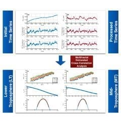
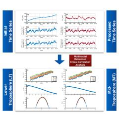
Multifractal Detrended Cross-Correlation Analysis of Global Methane and Temperature

by
Chris G. Tzanis
1,*,
Ioannis Koutsogiannis
1,
Kostas Philippopoulos
1 and
Nikolaos Kalamaras
2
1
Climate and Climatic Change Group, Section of Environmental Physics and Meteorology, Department of Physics, National and Kapodistrian University of Athens, 15784 Athens, Greece
2
Department of Weather Stations, Hellenic National Meteorological Service (HNMS), 16777 Athens, Greece
*
Author to whom correspondence should be addressed.
Remote Sens. 2020, 12(3), 557; https://doi.org/10.3390/rs12030557
Submission received: 30 December 2019 / Revised: 31 January 2020 / Accepted: 4 February 2020 / Published: 7 February 2020
(This article belongs to the Collection Feature Papers for Section Environmental Remote Sensing)

Abstract

:
Multifractal Detrended Cross-Correlation Analysis (MF-DCCA) was applied to time series of global methane concentrations and remotely-sensed temperature anomalies of the global lower and mid-troposphere, with the purpose of investigating the multifractal characteristics of their cross-correlated time series and examining their interaction in terms of nonlinear analysis. The findings revealed the multifractal nature of the cross-correlated time series and the existence of positive persistence. It was also found that the cross-correlation in the lower troposphere displayed more abundant multifractal characteristics when compared to the mid-troposphere. The source of multifractality in both cases was found to be mainly the dependence of long-range correlations on different fluctuation magnitudes. Multifractal Detrended Fluctuation Analysis (MF-DFA) was also applied to the time series of global methane and global lower and mid-tropospheric temperature anomalies to separately study their multifractal properties. From the results, it was found that the cross-correlated time series exhibit similar multifractal characteristics to the component time series. This could be another sign of the dynamic interaction between the two climate variables.

Graphical Abstract

1. Introduction

Climate change studies depend, to a great extent, on the examination of the relationship between different key components of the climate system. Atmospheric temperature and methane (CH4) are two of the most important parameters examined in climate research. Air temperature variability and trends at various atmospheric levels represent a crucial indicator of the warming or cooling of the Earth’s atmosphere both at a global and regional scale [1,2,3,4]. In addition, adequate and in-depth knowledge of temperature fluctuations is essential for validating the accuracy of climate models’ simulations [5,6,7]. The development of a climate data record of suitable length and reliability is required for the reliable detection of changes in the Earth’s atmospheric temperature [8]. In this respect, microwave soundings from space have proven successful in providing long-term temperature observations of the Earth’s atmosphere. Indeed, since the beginning of the satellite era in the late 1970s, atmospheric temperatures have been routinely monitored from space, until 2006 by the Microwave Sounding Unit (MSU), and later by its successor, the Advanced Microwave Sounding Unit (AMSU), which is fully operational since 1998. The MSU/AMSU microwave sounders are cross-scanning instruments onboard polar-orbiting weather satellites measuring the profile of temperature throughout the Earth’s atmosphere. Satellite observations of temperature at different levels of the Earth’s atmosphere are considered to be a valuable tool in climate change studies, since they provide high-resolution measurements with global coverage over a multidecadal time period [9].
Methane is a greenhouse gas with a significant contribution to the anthropogenic climate change having a strong decadal imprint [10,11,12]. Although it absorbs infrared radiation more effectively than carbon dioxide (CO2) [13,14], it remains in the Earth’s atmosphere for a relatively short period of time [15,16,17]. Methane is produced by both anthropogenic activities and natural processes. The greatest natural formation of CH4 occurs in wetlands due to the metabolic activity of anaerobic microorganisms under hypoxic conditions. CH4 production in natural wetlands is responsible for approximately 30% of its total emissions [18]. The anthropogenic sources of CH4 include fugitive releases from solid materials used in the energy production industry, discharges from gas mining and its supply chain, as well as emissions that are related to agricultural activity, livestock farming, and waste treatment [19]. Anthropogenic activities are responsible for more than half of the CH4 production from land and oceans [18]. On the other hand, the reaction with the hydroxyl radical (OH) is considered to be the basic sink of atmospheric CH4, a process that is subject to interannual fluctuations [20]. Apart from destroying CH4, this reaction is one of the main sources of water vapor in the stratosphere [21]. Atmospheric CH4 concentrations have been systematically monitored through a global network of surface air-sampling stations [22]. An overall increase by a factor of 2.5 has been observed during the industrial era [23]. However, for reasons that still remain under scientific debate [24,25,26], global CH4 concentrations remained stagnant for almost a decade between the late 1990s and 2006 and experienced continuous growth ever since [27,28,29,30].
Conventional statistical methods, which include the autocorrelation function or spectral analysis, are not always capable of describing nonlinear processes that are characterized by non-stationarities. In addition, traditional statistical methods usually examine time series over a single time scale and neglect time series features over multiple time scales. The development of fractal theory has fortunately offered robust alternatives for overcoming such limitations. The application of fractal methodology relies on the segmentation of a time series into self-similar parts and the exploration of the power-law behavior that reflects the scaling characteristics of the system examined. Kantelhardt et al. [31] developed the MF-DFA to determine the scaling behavior of time series with statistical properties that vary temporally. MF-DFA is a robust methodology and a valuable tool for time series analysis from a non-linear perspective [32,33,34,35,36,37,38,39,40]. Podobnik and Stanley [41] introduced the Detrended Cross-Correlation Analysis to detect the scaling properties in the cross-correlations between synchronous non-stationary time series. Their methodology has found application in a variety of scientific fields, including finance, physics, and earth sciences [42,43,44,45,46]. Finally, Zhou [47] proposed the Multifractal Detrended Cross-Correlation Analysis (MF-DCCA) to study the multifractal characteristics in cross-correlations of two nonstationary signals. MF-DCCA has been used in [48] to examine the cross-correlations between meteorological parameters and air pollution, and in [49] to explore the cross-correlations between sunspot numbers and river flow fluctuations from a multifractal perspective. Recently, Kar et al. [50] also used the MF-DCCA between soil radon concentrations and land surface temperature. This study focuses on the detection of cross-correlation scaling properties of global CH4 and remotely-sensed global temperature anomalies, both in the lower and mid-troposphere. Thus, MF-DCCA was adopted for these two significant components of the climate system to examine whether positive correlation exists between them throughout the Earth’s atmosphere.

2. Materials and Methods
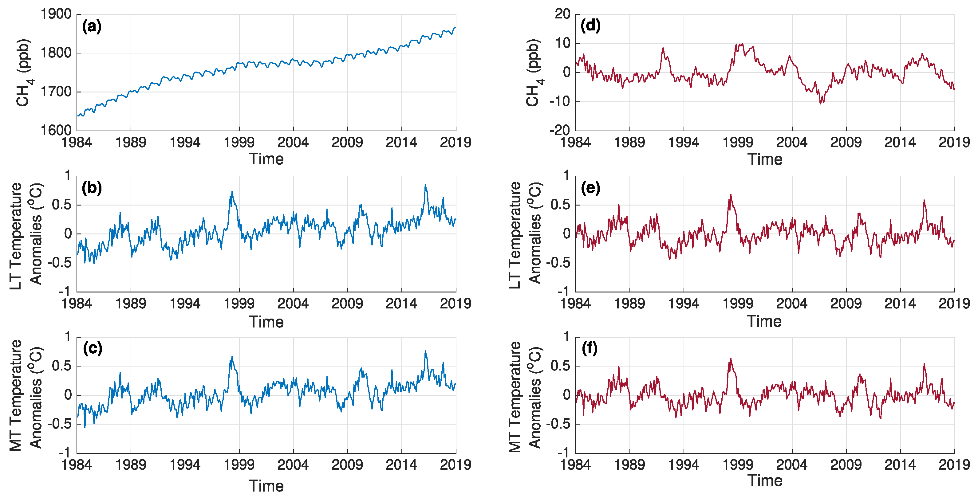
2.1. Data

Global mean monthly air temperature anomalies throughout the lower and mid-troposphere were used over the period 1984–2018. The temperature anomalies data were acquired from Version 6.0 of the University of Alabama in Huntsville (UAH) satellite temperature record [51]. The UAH dataset is based on observations performed by the MSU and its successor, the AMSU. The instruments, which operate between 50 and 60 GHz, use microwave radiometry, in order to detect the thermal microwave radiance that is emitted by oxygen (O2). Measurements of molecular oxygen’s microwave emission are used to estimate the weighted averages of temperature at three extensive atmospheric layers, namely the lower troposphere (LT), the mid-troposphere (MT) and the lower stratosphere. In general, oxygen concentration remains relatively constant in the atmosphere and, consequently, O2 is considered a secure temperature tracer. Details concerning the instruments’ calibration, data adjustments, and new processing methodologies, which are associated with the version 6.0 of the dataset, are further discussed in [51].
Globally-averaged mean monthly data of atmospheric CH4 dry air mole fractions, expressed as parts per billion (ppb), were also acquired from NOAA’s Earth’s System Research Laboratory (ESRL) for the same period (1984–2018). The global average values of CH4 are estimated through weekly measurements from a subset of ESRL’s global network of air sampling sites [52]. This subset includes surface stations at remote sites with a well-mixed marine boundary layer (MBL), whereas stations, where altitude and anthropogenic or natural sources and sinks could affect the observations, are excluded. The averaging methodology [53] involves fitting a smooth curve to the data at each site to diminish the impact of synoptic atmospheric phenomena and data gaps, plotting the latitudinal distribution of the smoothed values for weekly time steps per year and finally calculating the global means from the latitude plot. Detailed information regarding the data uncertainties and processing strategy can be found in [52,54].
The CH4 values and LT and MT temperature anomalies data were initially detrended, using polynomial regression analysis (of third order) prior to the implementation of the MF-DFA and MF-DCCA methodologies. Furthermore, the annual and semi-annual seasonal components that were identified in the CH4 time series were eliminated, using the well-established Wiener filter [55]. Figure 1 depicts the initial and processed time series of global CH4 and global LT and MT temperature anomalies.

2.2. Methodology

2.2.1. Multifractal Detrended Fluctuation Analysis (MF-DFA)

The multifractal properties for each parameter were investigated with MF-DFA [31]. The basic steps of the method are the following:
1. The profile X(i) is firstly constructed:
X ( i ) = k = 1 i [ x k x ]
where by xk and < x > the time series and its mean value are designated, respectively. The upper bound of summation i takes values from 1 to N, which corresponds to the length of the time series.
2. X(i) is partitioned into an integer number of NS = int(N/s) non-intersecting segments, all of which have the same length s, i.e., time scale. However, for time series with length N not divisible exactly by s, not all profile points will be considered. For this reason, the segmentation procedure is also repeated for the retrograde time series of the profile. Thus, we get 2NS segments in total.
3. Within each segment, a second-order (m = 2) polynomial X ˜ v is fitted to the profile, representing the local trend, where v = 1, …, 2NS is the number of each segment. The local trend is then subtracted from the profile and, thus, second-order trends are eliminated from the profile.
4. The detrended variance F2(s,v) is then calculated:
F 2 ( s , v ) = { 1 s i = 1 s { X [ ( v 1 ) s + i ] X ˜ v   ( i ) } 2 , f o r   v = 1 , , N s 1 s i = 1 s { X [ ( N ( v N s ) s + i ] X ˜ v   ( i ) } 2 , f o r   v = N s + 1 , , 2 N s
5. Considering the average of all segments, we get the qth order fluctuation function:
F q ( s ) = { 1 2 N S v = 1 2 N s [ F 2 ( s , v ) ] q 2 } 1 q
For q = 0, we have,
F 0 ( s ) = e x p ( 1 4 N S v = 1 2 N s l n [ F 2 ( s , v ) ] )
Fq(s) is determined only for sm+2. For q = 2, the MF-DFA results are identical to the DFA procedure [56,57,58,59,60].
6. Fq(s) is computed for all values of s. The scaling behavior of Fq(s) is examined through the plot of log(Fq(s)) against log(s) for each moment q. For time series that are long-range correlated, Fq(s) follows a power law:
F q ( s ) s h ( q )
For monofractal time series, the scaling exponent h(q) remains constant and it is equal to the Hurst exponent H. For multifractal time series, h(q) depends strongly on q, i.e., the scaling behavior is different for fluctuations of different magnitude. In these cases, h(q) is the generalized form of the Hurst exponent. For q > 0, h(q) reflects the scaling characteristics of partitions with large fluctuations. On the other hand, for q < 0, h(q) reflects the scaling properties of partitions with small fluctuations.
Ignoring the dependency of h(q) on q and supposing that h(q) = H, for values of H between 0 and 0.5, the time series is characterized by long-range negative correlation, denoting an anti-persistent character; for H > 0.5, it is characterized by long-range positive correlation (persistent behavior); for H = 0.5 it is considered to be uncorrelated, i.e., white noise.
Using the relationship τ(q) = qh(q)−1 and applying a Legendre transformation, we get
τ ( q ) = α
Additionally,
f ( a ) = q α τ ( q ) = q [ α h ( q ) ] + 1
The entity α describes the singularity strength, while f(α) represents the subset of the time series that is characterized by α. The plot of f(α) against α is the multifractal spectrum and it provides insights regarding the multifractal traits of the time series. The value of f(α) reaches its peak when the derivative of f(α) with respect to α equals zero, i.e., d f(α)/dα = 0. From Equation (7), this happens for q = 0 and, thus, f(α)max equals 1. When the above condition is satisfied, α is called the dominant Hurst exponent α0 and corresponds to the prevailing scaling behavior. Along with α0, the spectral width is also a key feature. It can be estimated by fitting a second-order polynomial around α0, as proposed by [61] and measuring the distance between αmax and αmin, the two points where the fitting curve intersects the horizontal axis:
P ( α ) = A ( α α 0 ) 2 + B ( α α 0 ) + C
A multifractal spectrum with a broad width indicates rich multifractality in the time series. On the other hand, smaller widths are associated with a more monofractal character of the time series. Furthermore, another aspect of the multifractal spectrum’s shape is its truncation type. The left side of the curve corresponds to positive values of q, whereas the right side of the curve is related to the negative values of q. Thus, a left-truncated spectrum indicates a multifractal structure with insensitivity to the large local fluctuations. A right-truncated spectrum, on the other hand, indicates a multifractal structure that is insensitive to the small local fluctuations. Finally, a symmetrical multifractal spectrum suggests that the time series shows the same sensitivity to both small and large local fluctuations.

2.2.2. Multifractal Detrended Cross-Correlation Analysis (MF-DCCA)

The MF-DCCA method [47] is used to measure the long-range cross-correlations between two time series, xk and yk, of equal length N. Steps 1–3 are similar to MF-DFA and they are applied for each time series, separately. Subsequently, their detrended covariance is determined:
F 2 ( s , v ) = { 1 s i = 1 s { X [ ( v 1 ) s + i ] X ˜ v ( i ) }   { Y [ ( v 1 ) s + i ] Y ˜ v ( i ) } , f o r   v = 1 , , N s 1 s i = 1 s { X [ ( N ( v N s ) s + i ] X ˜ v ( i ) } { Y [ ( N ( v N s ) s + i ] Y ˜ v ( i ) } , f o r   v = N s + 1 , , 2 N s
While considering the average of all segments, the qth order fluctuation function of the detrended covariance is calculated:
F q ( s ) = { 1 2 N S v = 1 2 N s [ F 2 ( v , s ) ] q 2 } 1 q
For q = 0, we get
F 0 ( s ) = e x p ( 1 4 N S v = 1 2 N s l n [ F 2 ( v , s ) ] )
Similarly to the MF-DFA analysis, the scaling behavior of the covariance fluctuations is examined by analyzing the plot of log(Fq(s)) versus log(s). A long-range correlation is inferred if the fluctuation function of the covariance is related to time scale via a power law, i.e.,
F q ( s ) s h x y ( q )
In this case, hxy represents the cross-correlation exponent. For x = y, that is, the two time series are identical, the procedure is simplified to MF-DFA. For hxy > 0.5, increasing values of one time series are expected to be followed by increasing values of the other (persistent behavior). For 0 < hxy < 0.5, increasing values of one time series are expected to be followed by decreasing values of the other (antipersistent behavior). Finally, for hxy = 0.5, the two time series are considered to be long-range uncorrelated. The discussion concerning the multifractal spectrum characteristics, mentioned at the MF-DFA method description, is also valid for the MF-DCCA spectrum.
Finally, the source of multifractality is an important issue that should be examined when coping with multifractal systems. The multifractal characteristics of a time series may derive either from a broad probability density function or from different long-range correlations. The origins of multifractality can be investigated by randomly reordering (shuffling) the values of the two time series prior to applying MF-DFA and MF-DCCA. If the multifractal properties are strongly preserved, then multifractality in the time series originates from a broad probability density function. On the other hand, if the multifractality is prominently diminished, then multifractal properties mainly originate from long-range correlations of different fluctuation magnitudes.

3. Results and Discussion
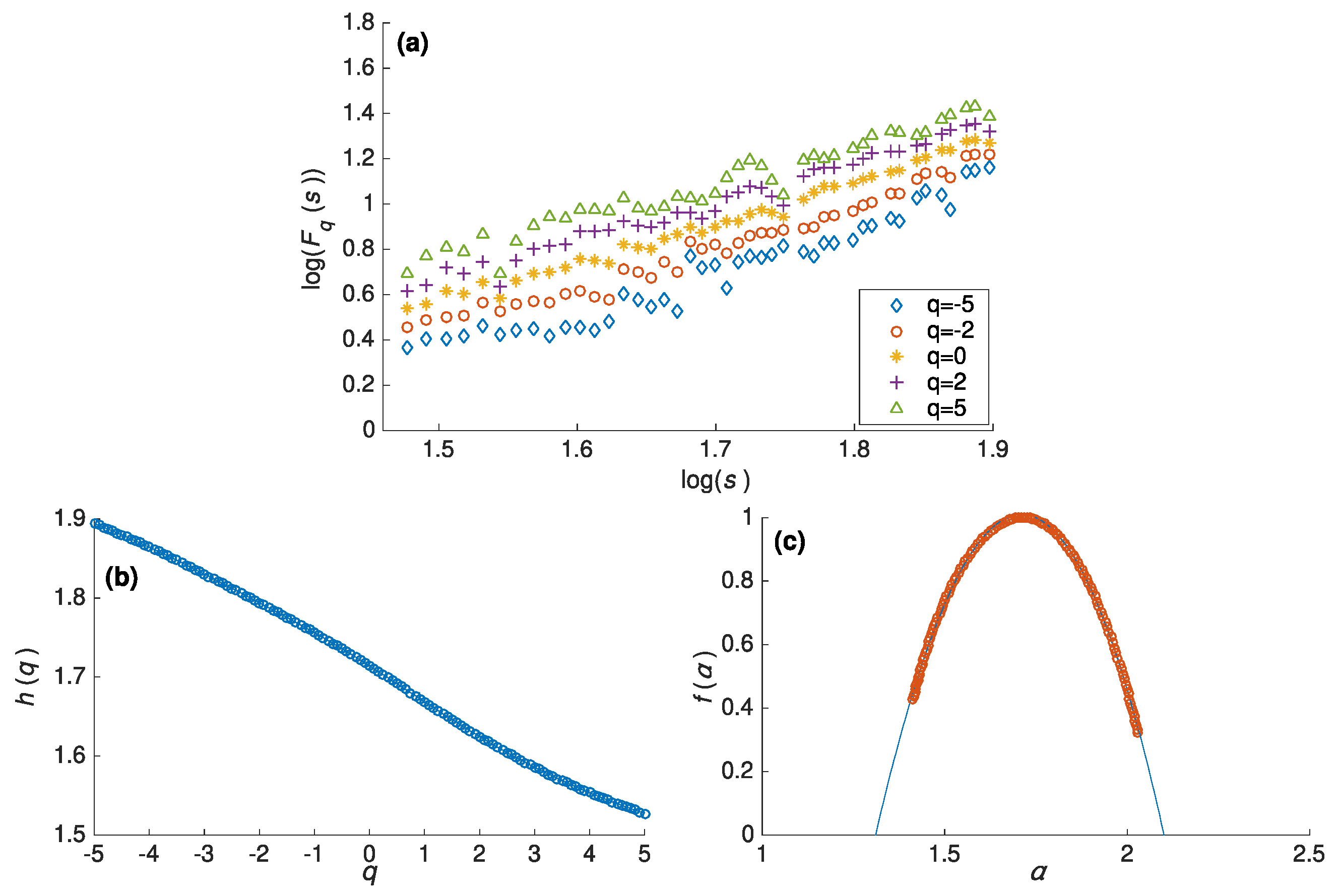
3.1. MF-DFA Results

Herein, MF-DFA is applied on the time series of global methane and global LT and MT temperature anomalies and the findings are discussed. Indicatively, Figure 2 illustrates the plots that are derived from the MF-DFA analysis on the detrended and deseasonalized values of global CH4. The three types of plots are the plot of log(Fq(s)) against log(s) (Figure 2a), the plot of h(q) against q (Figure 2b), and the multifractal spectrum f(a) against α (Figure 2c). The time scales used both in the MF-DFA and MF-DCCA range between 30 months (s ≈ 101.5) and N/5, i.e., 84 months (s ≈ 101.9), where, by N, the length of the time series is represented. The values of q also range from −5 to +5 by steps of 0.1. From the examination of Figure 2a, it is observed that log(Fq(s)) linearly increases with log(s). It is important to mention that the slopes are different for each q; this is a sign that the time series of CH4 display multifractal characteristics.
Furthermore, by computing the slopes of Fq(s) for each q, the values of h(q) are estimated. From Figure 2b, it can be observed that h(q) depends on q. This also reveals the multifractal character of CH4. In addition, h(q) > 0.5 for all moments q, and, therefore, long-range positive correlations are identified in the CH4 time series. Moreover, it can be noted that the values of h(q) for q < 0 are greater than the corresponding values for q > 0. This result permits to assume that the small fluctuations (q < 0) display more abundant multifractal features and, therefore, a greater level of complexity than the large fluctuations (q > 0). The application of MF-DFA to the time series of both LT and MT temperature anomalies produced similar results. The presence of scaling features and multifractality in temperature time series is well documented [38,39,62,63].
Significant information concerning the multifractal properties can also be acquired from the singularity spectra of CH4, LT, and MT temperature anomalies (Table 1). The values of α0 for the three climate variables are 1.714, 1.387, and 1.441, respectively. Thus, α0 > 0.5 for all parameters, which signifies that they have positive long-range correlations. The corresponding w values are 0.790, 1.108, and 1.128, respectively, which reflects that the temperature anomalies time series show higher levels of multifractality when compared to CH4. This finding further highlights the importance of examining their cross-correlation scaling properties for the study of the climate system dynamics. The global temperature is regulated by global energy balance and its fluctuations are influenced by multi-scale complex interactions of atmospheric processes and a number of climate factors (e.g., solar radiation, greenhouse gasses, aerosols, planetary albedo, and clouds) [64,65,66,67]. On the other hand, methane affects the climate directly and indirectly via chemical reactions [68].

3.2. MF-DCCA Results

3.2.1. Lower Troposphere

In this section, the results of the application of the MF-DCCA procedure are presented. MF-DCCA was initially applied to reveal the multifractal structure of the cross-correlations between global CH4 and temperature anomalies of the global LT. Figure 3a portrays the way that log(Fq(s)) changes with log(s) for a multitude of moments q. It can be observed from the plot that log(Fq(s)) increases linearly with log(s). Therefore, Fq(s) and s are related with a power-law mechanism. The values of hxy(q) were obtained, in a similar way to the MF-DFA procedure using a linear fit. Figure 3b depicts the graphical representation of hxy(q) against q. It is clear that hxy(q) decreases with q. This is a sign of the presence of multifractality in the cross-correlations. All of the hxy(q) values were found to be greater than 0.5, which designates the positive persistence of the cross-correlated time series. At this point, it should be noticed that CH4 global concentration increases evoke a temperature increase. However, according to [69,70], the increase of temperature due to global warming is also likely to increase methanogenesis in wetlands, which is, among others, a significant source in the CH4 global cycle. Increased natural CH4 emissions from wetlands may trigger further increases in global temperature within this feedback loop. It can also be observed from Figure 3b that the values of hxy(q) are greater for negative moments q. Therefore, it is inferred that the cross-correlated time series show a stronger multifractal character for small fluctuations in contrast to large fluctuations. Figure 3c provides further information regarding the multifractal properties of the cross-correlated time series. More precisely, the parabolic shape and the multifractal spectral width confirm the presence of rich multifractality. Additionally, no prominent signs of truncation are evident from a visual inspection of the plot. The symmetric shape of the parabola denotes that the cross-correlated time series exhibits equal sensitivity to the small and large local fluctuations. Table 1 depicts the main multifractal characteristics and their values. It can be observed that both values of αο and w of the cross-correlated time series lie between the corresponding values of the initial time series.

3.2.2. Mid-Troposphere

MF-DCCA was also applied between global CH4 and temperature anomalies of the global MT to explore the cross-correlations of global CH4 and temperature anomalies at higher levels in the Earth’s atmosphere and compare their multifractal characteristics with those of the lower troposphere. A power-law mechanism can be distinguished from the inspection of the log(Fq(s)) plot against log(s) (Figure 3d). Furthermore, hxy(q) decreases with increasing q (Figure 3e). Thus, hxy(q) depends on q, which is a strong manifestation of multifractality. Moreover, hxy(q) > 0.5 for all values of q, which implies the existence of positive persistence in accordance to the previous findings. Finally, the shape of the multifractal spectrum (Figure 3f) verifies the existence of multifractality. However, a notable distinction between Figure 3c,f is that the former is right truncated, i.e., the cross-correlations between global CH4 and global mid-tropospheric temperature anomalies have a structure that displays a greater sensitivity to the large local fluctuations. In addition, the spectral width in Figure 3f is smaller (w = 0.757) when compared to the width estimated in Figure 3c (w = 0.887) (Table 1). From this finding, it can be deduced that the temporal fluctuations of the cross-correlations between global methane and global temperature anomalies possess richer multifractal properties and, therefore, greater complexity in the LT than in the MT. This could be associated with the different degree of interaction between CH4 and temperature in the LT and MT as well as the above-mentioned different multifractal characteristics of LT and MT temperature.

3.2.3. Origins of Multifractality

In the preceding section, we verified the multifractal structure of the global CH4 concentrations and the global LT and MT temperature anomalies along with their cross-correlations. Herein, the possible origins of the exhibited multifractality are investigated. Generally, multifractality stems either from long-range correlations or a broad probability density function. The time series of CH4 and temperature anomalies were randomly reordered prior to the implementation of MF-DFA and MF-DCCA to detect the origins of the multifractal characteristics of the examined time series. The shuffling procedure was repeated 100 times and the average values of the produced parameters were calculated. From Figure 4a and Figure 5a,d, it can be seen that the plot of log(Fq(s)) against log(s) consists of straight parallel lines, which implies that the multifractal structure in the shuffled time series is destroyed. In addition, the dependence of h(q) and hxy(q) on q is very small. Their values in all shuffled time series are close to 0.5 (Figure 4 and Figure 5b,e). This also highlights the absence of rich multifractal properties. Furthermore, the width of the multifractal spectra is greatly reduced in the shuffled time series (Figure 4c and Figure 5c,f). In Table 2, the values of w and α0 for the shuffled time series are represented. Thus, while taking the above findings into account, it is deduced that a random shuffling of the values of the two climate parameters and their cross-correlations significantly weakens their multifractality. Consequently, it can be assumed that multifractality mainly stems from different long-range correlations for small and large fluctuations for the examined time scales.

4. Conclusions

In this work, global CH4 and remotely-sensed tropospheric temperature anomalies are analyzed using the MF-DCCA to study the multifractality of their cross-correlations. Initially, the LT and MT temperature anomalies were found to exhibit stronger multifractality when compared to global CH4. Furthermore, the values of the exponents h(q) of CH4 and tropospheric temperature along with the exponent hxy(q) of their cross-correlated time series, are all larger than 0.5 for all moments q, which is a clear indication of their positive persistent behavior. This indicates that the impact of past events has an influence on the succeeding values of the parameters. The spectral width is also indicative of the multifractality of the examined time series. Another important finding is that the α0 value of the cross-correlated time series lies between the α0 values of the two variables. Similarly, the value of the spectral width of the cross-correlated time series is between the corresponding values of the two parameters. This could be another sign of the interaction between the two climate variables from a nonlinear perspective. The scaling behavior of the cross-correlation between CH4 and the temperature anomalies of the global MT is weaker when compared to the LT. Finally, the outcome of the shuffling procedure in the cross-correlated time series suggest that multifractality originates mainly from different long-range correlations for small and large fluctuations.

Author Contributions

Conceptualization, C.G.T. and I.K.; methodology, C.G.T., I.K., K.P. and N.K.; software, C.G.T., I.K. and K.P.; validation, C.G.T., I.K., K.P. and N.K.; formal analysis, C.G.T., I.K., K.P. and N.K.; investigation, C.G.T., I.K., K.P. and N.K.; data curation, C.G.T., I.K., K.P. and N.K.; writing—original draft preparation, C.G.T., I.K. and N.K.; writing—review and editing, C.G.T., I.K., K.P. and N.K.; visualization, C.G.T. and I.K.; supervision, C.G.T. All authors have read and agreed to the published version of the manuscript.

Funding

This research received no external funding.

Acknowledgments

The authors would like to express their acknowledgements to Ed. Dlugokencky for the NOAA ESRL global methane data and the University of Alabama in Huntsville for the MSU/AMSU global temperature anomalies data.

Conflicts of Interest

The authors declare no conflict of interest.

References

  1. Santer, B.D.; Solomon, S.; Wentz, F.J.; Fu, Q.; Po-Chedley, S.; Mears, C.; Painter, J.F.; Bonfils, C. Tropospheric Warming over the Past Two Decades. Sci. Rep. 2017, 7, 2336. [Google Scholar] [CrossRef]
  2. Hawkins, E.; Ortega, P.; Suckling, E.; Schurer, A.; Hegerl, G.; Jones, P.; Joshi, M.; Osborn, T.J.; Masson-Delmotte, V.; Mignot, J.; et al. Estimating Changes in Global Temperature since the Preindustrial Period. Bull. Am. Meteorol. Soc. 2017, 98, 1841–1856. [Google Scholar] [CrossRef]
  3. Thompson, D.W.J.; Seidel, D.J.; Randel, W.J.; Zou, C.-Z.; Butler, A.H.; Mears, C.; Osso, A.; Long, C.; Lin, R. The mystery of recent stratospheric temperature trends. Nature 2012, 491, 692–697. [Google Scholar] [CrossRef] [PubMed]
  4. Tzanis, C.G.; Koutsogiannis, I.; Philippopoulos, K.; Deligiorgi, D. Recent climate trends over Greece. Atmos. Res. 2019, 230, 104623. [Google Scholar] [CrossRef]
  5. Randel, W.J.; Polvani, L.; Wu, F.; Kinnison, D.E.; Zou, C.-Z.; Mears, C. Troposphere-Stratosphere Temperature Trends Derived From Satellite Data Compared With Ensemble Simulations From WACCM. J. Geophys. Res. Atmos. 2017, 122, 9651–9667. [Google Scholar] [CrossRef]
  6. Santer, B.D.; Fyfe, J.C.; Pallotta, G.; Flato, G.M.; Meehl, G.A.; England, M.H.; Hawkins, E.; Mann, M.E.; Painter, J.F.; Bonfils, C.; et al. Causes of differences in model and satellite tropospheric warming rates. Nat. Geosci. 2017, 10, 478–485. [Google Scholar] [CrossRef]
  7. Santer, B.D.; Solomon, S.; Pallotta, G.; Mears, C.; Po-Chedley, S.; Fu, Q.; Wentz, F.; Zou, C.-Z.; Painter, J.; Cvijanovic, I.; et al. Comparing Tropospheric Warming in Climate Models and Satellite Data. J. Clim. 2017, 30, 373–392. [Google Scholar] [CrossRef]
  8. National Research Council. Climate Data Records from Environmental Satellites: Interim Report; The National Academies Press: Washington, DC, USA, 2004. [Google Scholar]
  9. Christy, J.R.; Spencer, R.W.; Braswell, W.D.; Junod, R. Examination of space-based bulk atmospheric temperatures used in climate research. Int. J. Remote Sens. 2018, 39, 3580–3607. [Google Scholar] [CrossRef] [Green Version]
  10. IPCC. Climate Change 2013: The Physical Science Basis. Contribution of Working Group I to the Fifth Assessment Report of the Intergovernmental Panel on Climate Change; Stocker, T.F., Qin, D., Plattner, G.-K., Tignor, M., Allen, S.K., Boschung, J., Nauels, A., Xia, Y., Bex, V., Midgley, P.M., Eds.; Cambridge University Press: Cambridge, UK; New York, NY, USA, 2013; 1535p. [Google Scholar]
  11. Etminan, M.; Myhre, G.; Highwood, E.J.; Shine, K.P. Radiative forcing of carbon dioxide, methane, and nitrous oxide: A significant revision of the methane radiative forcing. Geophys. Res. Lett. 2016, 43, 12614–12623. [Google Scholar] [CrossRef]
  12. Allen, M.R.; Shine, K.P.; Fuglestvedt, J.S.; Millar, R.J.; Cain, M.; Frame, D.J.; Macey, A.H. A solution to the misrepresentations of CO2-equivalent emissions of short-lived climate pollutants under ambitious mitigation. npj Clim. Atmos. Sci. 2018, 1, 16. [Google Scholar] [CrossRef]
  13. Azar, C.; Johansson, D.J.A. On the relationship between metrics to compare greenhouse gases; the case of IGTP, GWP and SGTP. Earth Syst. Dyn. 2012, 3, 139–147. [Google Scholar] [CrossRef] [Green Version]
  14. Myhre, G.; Shindell, D.; Bréon, F.-M.; Collins, W.D.; Fuglestvedt, J.; Huang, J.; Koch, D.; Lamarque, J.-F.; Lee, D.; Mendoza, B.; et al. Anthropogenic and Natural Radiative Forcing. In Climate Change 2013—The Physical Science Basis; Stocker, T., Ed.; Intergovernmental Panel on Climate Change; Cambridge University Press: Cambridge, UK, 2013; pp. 659–740. [Google Scholar]
  15. Prather, M.J.; Holmes, C.D.; Hsu, J. Reactive greenhouse gas scenarios: Systematic exploration of uncertainties and the role of atmospheric chemistry. Geophys. Res. Lett. 2012, 39, L09803. [Google Scholar] [CrossRef] [Green Version]
  16. Fiore, A.M.; Dentener, F.J.; Wild, O.; Cuvelier, C.; Schultz, M.G.; Hess, P.; Textor, C.; Schulz, M.; Doherty, R.M.; Horowitz, L.W.; et al. Multimodel estimates of intercontinental source-receptor relationships for ozone pollution. J. Geophys. Res. 2009, 114, D04301. [Google Scholar] [CrossRef]
  17. Voulgarakis, A.; Naik, V.; Lamarque, J.-F.; Shindell, D.T.; Young, P.J.; Prather, M.J.; Wild, O.; Field, R.D.; Bergmann, D.; Cameron-Smith, P.; et al. Analysis of present day and future OH and methane lifetime in the ACCMIP simulations. Atmos. Chem. Phys. 2013, 13, 2563–2587. [Google Scholar] [CrossRef] [Green Version]
  18. Kirschke, S.; Bousquet, P.; Ciais, P.; Saunois, M.; Canadell, J.G.; Dlugokencky, E.J.; Bergamaschi, P.; Bergmann, D.; Blake, D.R.; Bruhwiler, L.; et al. Three decades of global methane sources and sinks. Nat. Geosci. 2013, 6, 813–823. [Google Scholar] [CrossRef]
  19. Saunois, M.; Bousquet, P.; Poulter, B.; Peregon, A.; Ciais, P.; Canadell, J.G.; Dlugokencky, E.J.; Etiope, G.; Bastviken, D.; Houweling, S.; et al. The global methane budget 2000–2012. Earth Syst. Sci. Data 2016, 8, 697–751. [Google Scholar] [CrossRef] [Green Version]
  20. Holmes, C.D.; Prather, M.J.; Søvde, O.A.; Myhre, G. Future methane, hydroxyl, and their uncertainties: Key climate and emission parameters for future predictions. Atmos. Chem. Phys. 2013, 13, 285–302. [Google Scholar] [CrossRef] [Green Version]
  21. Frank, F.; Jöckel, P.; Gromov, S.; Dameris, M. Investigating the yield of H2O and H2 from methane oxidation in the stratosphere. Atmos. Chem. Phys. 2018, 13, 9955–9973. [Google Scholar] [CrossRef] [Green Version]
  22. Dlugokencky, E.J.; Nisbet, E.G.; Fisher, R.; Lowry, D. Global atmospheric methane: Budget, changes and dangers. Philos. Trans. R. Soc. A Math. Phys. Eng. Sci. 2011, 369, 2058–2072. [Google Scholar] [CrossRef] [Green Version]
  23. Hartmann, D.L. Global Physical Climatology, 2nd ed.; Elsevier: Waltham, MA, USA, 2016; ISBN 9780123285317. [Google Scholar]
  24. Turner, A.J.; Frankenberg, C.; Wennberg, P.O.; Jacob, D.J. Ambiguity in the causes for decadal trends in atmospheric methane and hydroxyl. Proc. Natl. Acad. Sci. USA 2017, 114, 5367–5372. [Google Scholar] [CrossRef] [PubMed] [Green Version]
  25. Bergamaschi, P.; Houweling, S.; Segers, A.; Krol, M.; Frankenberg, C.; Scheepmaker, R.A.; Dlugokencky, E.; Wofsy, S.C.; Kort, E.A.; Sweeney, C.; et al. Atmospheric CH 4 in the first decade of the 21st century: Inverse modeling analysis using SCIAMACHY satellite retrievals and NOAA surface measurements. J. Geophys. Res. Atmos. 2013, 118, 7350–7369. [Google Scholar] [CrossRef] [Green Version]
  26. Bousquet, P.; Ringeval, B.; Pison, I.; Dlugokencky, E.J.; Brunke, E.-G.; Carouge, C.; Chevallier, F.; Fortems-Cheiney, A.; Frankenberg, C.; Hauglustaine, D.A.; et al. Source attribution of the changes in atmospheric methane for 2006–2008. Atmos. Chem. Phys. 2011, 11, 3689–3700. [Google Scholar] [CrossRef] [Green Version]
  27. Dlugokencky, E.J.; Bruhwiler, L.; White, J.W.C.; Emmons, L.K.; Novelli, P.C.; Montzka, S.A.; Masarie, K.A.; Lang, P.M.; Crotwell, A.M.; Miller, J.B.; et al. Observational constraints on recent increases in the atmospheric CH 4 burden. Geophys. Res. Lett. 2009, 36, L18803. [Google Scholar] [CrossRef] [Green Version]
  28. Nisbet, E.G.; Dlugokencky, E.J.; Bousquet, P. Methane on the Rise--Again. Science 2014, 343, 493–495. [Google Scholar] [CrossRef] [Green Version]
  29. Nisbet, E.G.; Dlugokencky, E.J.; Manning, M.R.; Lowry, D.; Fisher, R.E.; France, J.L.; Michel, S.E.; Miller, J.B.; White, J.W.C.; Vaughn, B.; et al. Rising atmospheric methane: 2007-2014 growth and isotopic shift. Glob. Biogeochem. Cycles 2016, 30, 1356–1370. [Google Scholar] [CrossRef] [Green Version]
  30. Rigby, M.; Prinn, R.G.; Fraser, P.J.; Simmonds, P.G.; Langenfelds, R.L.; Huang, J.; Cunnold, D.M.; Steele, L.P.; Krummel, P.B.; Weiss, R.F.; et al. Renewed growth of atmospheric methane. Geophys. Res. Lett. 2008, 35, L22805. [Google Scholar] [CrossRef] [Green Version]
  31. Kantelhardt, J.W.; Zschiegner, S.A.; Koscielny-Bunde, E.; Havlin, S.; Bunde, A.; Stanley, H.E. Multifractal detrended fluctuation analysis of nonstationary time series. Physica A 2002, 316, 87–114. [Google Scholar] [CrossRef] [Green Version]
  32. Sadegh Movahed, M.; Hermanis, E. Fractal analysis of river flow fluctuations. Phys. A 2008, 387, 915–932. [Google Scholar] [CrossRef] [Green Version]
  33. Movahed, M.S.; Jafari, G.R.; Ghasemi, F.; Rahvar, S.; Tabar, M.R.R. Multifractal detrended fluctuation analysis of sunspot time series. J. Stat. Mech. Theory Exp. 2006, 2006, P02003. [Google Scholar] [CrossRef] [Green Version]
  34. Baranowski, P.; Krzyszczak, J.; Slawinski, C.; Hoffmann, H.; Kozyra, J.; Nieróbca, A.; Siwek, K.; Gluza, A. Multifractal analysis of meteorological time series to assess climate impacts. Clim. Res. 2015, 65, 39–52. [Google Scholar] [CrossRef] [Green Version]
  35. Zhou, Y.; Zhang, Q.; Singh, V.P. Fractal-based evaluation of the effect of water reservoirs on hydrological processes: The dams in the Yangtze River as a case study. Stoch. Environ. Res. Risk Assess. 2014, 28, 263–279. [Google Scholar] [CrossRef]
  36. Du, H.; Wu, Z.; Zong, S.; Meng, X.; Wang, L. Assessing the characteristics of extreme precipitation over northeast China using the multifractal detrended fluctuation analysis. J. Geophys. Res. Atmos. 2013, 118, 6165–6174. [Google Scholar] [CrossRef]
  37. Xue, Y.; Pan, W.; Lu, W.-Z.; He, H.-D. Multifractal nature of particulate matters (PMs) in Hong Kong urban air. Sci. Total Environ. 2015, 532, 744–751. [Google Scholar] [CrossRef] [PubMed]
  38. Kalamaras, N.; Philippopoulos, K.; Deligiorgi, D.; Tzanis, C.G.; Karvounis, G. Multifractal scaling properties of daily air temperature time series. Chaos Solitons Fractals 2017, 98, 38–43. [Google Scholar] [CrossRef]
  39. Kalamaras, N.; Tzanis, C.G.; Deligiorgi, D.; Philippopoulos, K.; Koutsogiannis, I. Distribution of air temperature multifractal characteristics over Greece. Atmosphere 2019, 10, 45. [Google Scholar] [CrossRef] [Green Version]
  40. Philippopoulos, K.; Kalamaras, N.; Tzanis, C.G.; Deligiorgi, D.; Koutsogiannis, I. Multifractal Detrended Fluctuation Analysis of temperature reanalysis data over Greece. Atmosphere 2019, 10, 336. [Google Scholar] [CrossRef] [Green Version]
  41. Podobnik, B.; Stanley, H.E. Detrended Cross-Correlation Analysis: A New Method for Analyzing Two Nonstationary Time Series. Phys. Rev. Lett. 2008, 100, 084102. [Google Scholar] [CrossRef] [Green Version]
  42. Gvozdanovic, I.; Podobnik, B.; Wang, D.; Eugene Stanley, H. 1/f behavior in cross-correlations between absolute returns in a US market. Physica A 2012, 391, 2860–2866. [Google Scholar] [CrossRef]
  43. Horvatic, D.; Stanley, H.E.; Podobnik, B. Detrended cross-correlation analysis for non-stationary time series with periodic trends. Europhys. Lett. 2011, 94, 18007. [Google Scholar] [CrossRef] [Green Version]
  44. Marinho, E.B.S.; Sousa, A.M.Y.R.; Andrade, R.F.S. Using Detrended Cross-Correlation Analysis in geophysical data. Phys. A 2013, 392, 2195–2201. [Google Scholar] [CrossRef] [Green Version]
  45. Shen, C.; Li, C.; Si, Y. A detrended cross-correlation analysis of meteorological and API data in Nanjing, China. Phys. A 2015, 419, 417–428. [Google Scholar] [CrossRef]
  46. Liao, W.; Wang, X.; Fan, Q.; Zhou, S.; Chang, M.; Wang, Z.; Wang, Y.; Tu, Q. Long-term atmospheric visibility, sunshine duration and precipitation trends in South China. Atmos. Environ. 2015, 107, 204–216. [Google Scholar] [CrossRef]
  47. Zhou, W.-X. Multifractal detrended cross-correlation analysis for two nonstationary signals. Phys. Rev. E 2008, 77, 066211. [Google Scholar] [CrossRef] [PubMed] [Green Version]
  48. Zhang, C.; Ni, Z.; Ni, L. Multifractal detrended cross-correlation analysis between PM2.5 and meteorological factors. Phys. A 2015, 438, 114–123. [Google Scholar] [CrossRef]
  49. Hajian, S.; Movahed, M.S. Multifractal Detrended Cross-Correlation Analysis of sunspot numbers and river flow fluctuations. Phys. A 2010, 389, 4942–4957. [Google Scholar] [CrossRef] [Green Version]
  50. Kar, A.; Chatterjee, S.; Ghosh, D. Multifractal detrended cross-correlation analysis of Land-surface temperature anomalies and Soil radon concentration. Phys. A 2019, 521, 236–247. [Google Scholar] [CrossRef]
  51. Spencer, R.W.; Christy, J.R.; Braswell, W.D. UAH Version 6 global satellite temperature products: Methodology and results. Asia-Pac. J. Atmos. Sci. 2017, 53, 121–130. [Google Scholar] [CrossRef]
  52. Dlugokencky, E.J.; Steele, L.P.; Lang, P.M.; Masarie, K.A. The growth rate and distribution of atmospheric methane. J. Geophys. Res. 1994, 99, 17021. [Google Scholar] [CrossRef]
  53. Masarie, K.A.; Tans, P.P. Extension and integration of atmospheric carbon dioxide data into a globally consistent measurement record. J. Geophys. Res. 1995, 100, 11593. [Google Scholar] [CrossRef] [Green Version]
  54. Ed Dlugokencky, NOAA/ESRL. Available online: https://www.esrl.noaa.gov/gmd/ccgg/trends_ch4/ (accessed on 13 November 2019).
  55. Wiener, N. Extrapolation, Interpolation, and Smoothing of Stationary Time Series; The MIT Press: Cambridge, MA, USA, 1964. [Google Scholar]
  56. Sarlis, N.V.; Skordas, E.S.; Varotsos, P.A. Order parameter fluctuations of seismicity in natural time before and after mainshocks. EPL 2010, 91, 59001. [Google Scholar] [CrossRef]
  57. Skordas, E.S.; Sarlis, N.V.; Varotsos, P.A. Effect of significant data loss on identifying electric signals that precede rupture estimated by detrended fluctuation analysis in natural time. Chaos 2010, 20, 033111. [Google Scholar] [CrossRef] [PubMed] [Green Version]
  58. Varotsos, C.A.; Tzanis, C. A new tool for the study of the ozone hole dynamics over Antarctica. Atmos. Environ. 2012, 47, 428–434. [Google Scholar] [CrossRef]
  59. Chattopadhyay, G.; Chattopadhyay, S. Study on statistical aspects of monthly sunspot number time series and its long-range correlation through detrended fluctuation analysis. Indian J. Phys. 2014, 88, 1135–1140. [Google Scholar] [CrossRef]
  60. Varotsos, C.A.; Lovejoy, S.; Sarlis, N.V.; Tzanis, C.G.; Efstathiou, M.N. On the scaling of the solar incident flux. Atmos. Chem. Phys. 2015, 15, 7301–7306. [Google Scholar] [CrossRef] [Green Version]
  61. Shimizu, Y.; Thurner, S.; Ehrenberger, K. Multifractal spectra as a measure of complexity in human posture. Fractals 2002, 10, 103–116. [Google Scholar] [CrossRef]
  62. Varotsos, C.A.; Efstathiou, M.N. Has global warming already arrived? J. Atmos. Sol.-Terr. Phys. 2019, 182, 31–38. [Google Scholar] [CrossRef]
  63. Mali, P. Multifractal characterization of global temperature anomalies. Theor. Appl. Climatol. 2015, 121, 641–648. [Google Scholar] [CrossRef]
  64. Tzanis, C. On the relationship between total ozone and temperature in the troposphere and the lower stratosphere. Int. J. Remote Sens. 2009, 30, 6075–6084. [Google Scholar] [CrossRef]
  65. Amanollahi, J.; Tzanis, C.; Ramli, M.F.; Abdullah, A.M. Urban heat evolution in a tropical area utilizing Landsat imagery. Atmos. Res. 2016, 167, 175–182. [Google Scholar] [CrossRef]
  66. Varotsos, C.A.; Melnikova, I.N.; Cracknell, A.P.; Tzanis, C.; Vasilyev, A.V. New spectral functions of the near-ground albedo derived from aircraft diffraction spectrometer observations. Atmos. Chem. Phys. 2014, 14, 6953–6965. [Google Scholar] [CrossRef] [Green Version]
  67. Tzanis, C.; Varotsos, C.A. Tropospheric aerosol forcing of climate: A case study for the greater area of Greece. Int. J. Remote Sens. 2008, 29, 2507–2517. [Google Scholar] [CrossRef]
  68. Lelieveld, J.; Crutzen, P.J. Indirect chemical effects of methane on climate warming. Nature 1992, 355, 339–342. [Google Scholar] [CrossRef]
  69. Cui, M.; Ma, A.; Qi, H.; Zhuang, X.; Zhuang, G.; Zhao, G. Warmer temperature accelerates methane emissions from the Zoige wetland on the Tibetan Plateau without changing methanogenic community composition. Sci. Rep. 2015, 5, 11616. [Google Scholar] [CrossRef] [PubMed] [Green Version]
  70. Dean, J.F.; Middelburg, J.J.; Röckmann, T.; Aerts, R.; Blauw, L.G.; Egger, M.; Jetten, M.S.M.; de Jong, A.E.E.; Meisel, O.H.; Rasigraf, O.; et al. Methane Feedbacks to the Global Climate System in a Warmer World. Rev. Geophys. 2018, 56, 207–250. [Google Scholar] [CrossRef]
Figure 1. Time series of initial (ac) and processed (df) global CH4 and temperature anomalies of the lower troposphere (LT) and mid-troposphere (MT).
Remotesensing 12 00557 g001
Figure 2. Multifractal Detrended Fluctuation Analysis (MF-DFA) results for global CH4; (a) Plot of log(Fq(s)) against log(s); (b) Plot of h(q) against q; and, (c) Multifractal spectrum f(a) against a.
Remotesensing 12 00557 g002
Figure 3. Multifractal Detrended Cross-Correlation Analysis (MF-DCCA) results between global CH4 and global LT (left) and MT (right) temperature anomalies; (a,d) Plots of log(Fq(s)) against log(s); (b,e) Plot of hxy(q) against q; and, (c,f) Multifractal spectrum f(a) against a.
Remotesensing 12 00557 g003
Figure 4. Multifractal Detrended Fluctuation Analysis (MF-DFA) results for the shuffled series of global CH4; (a) Plot of log(Fq(s)) against log(s); (b) Plot of hxy(q) against q; (c) Multifractal spectrum f(a) against a.
Remotesensing 12 00557 g004
Figure 5. Multifractal Detrended Cross-Correlation Analysis (MF-DCCA) plots for the shuffled series between global CH4 and global LT (left) and MT (right) temperature anomalies; (a,d) Plot of log(Fq(s)) against log(s); (b,e) Plot of hxy(q) against q; and, (c,f) Multifractal spectrum f(a) against a.
Remotesensing 12 00557 g005
Table 1. Multifractal characteristics for CH4 and temperature anomalies of the global LT and MT along with their cross-correlations (CC).
ParameterCH4Temperature Anomalies (LT)Temperature Anomalies (MT)CC (LT)CC (MT)
α01.7141.3871.4411.5581.582
w0.7901.1081.1280.8870.757
Table 2. Multifractal characteristics for the shuffled time series of global CH4 and the temperature anomalies of the global LT and MT and their cross-correlations (CC).
ParameterCH4Temperature Anomalies (LT)Temperature Anomalies (MT)CC (LT)CC (MT)
α00.5080.5270.5080.5240.500
w0.2880.2650.2800.2290.317

