Review

Remote Sensing in Agriculture—Accomplishments, Limitations, and Opportunities

Department of Food, Agricultural and Biological Engineering, The Ohio State University, Columbus, OH 43210, USA
*
Author to whom correspondence should be addressed.
Remote Sens. 2020, 12(22), 3783; https://doi.org/10.3390/rs12223783
Submission received: 5 October 2020 / Revised: 5 November 2020 / Accepted: 11 November 2020 / Published: 19 November 2020
(This article belongs to the Special Issue Remote Sensing and IoT for Smart Learning Environments)

Abstract

:
Remote sensing (RS) technologies provide a diagnostic tool that can serve as an early warning system, allowing the agricultural community to intervene early on to counter potential problems before they spread widely and negatively impact crop productivity. With the recent advancements in sensor technologies, data management and data analytics, currently, several RS options are available to the agricultural community. However, the agricultural sector is yet to implement RS technologies fully due to knowledge gaps on their sufficiency, appropriateness and techno-economic feasibilities. This study reviewed the literature between 2000 to 2019 that focused on the application of RS technologies in production agriculture, ranging from field preparation, planting, and in-season applications to harvesting, with the objective of contributing to the scientific understanding on the potential for RS technologies to support decision-making within different production stages. We found an increasing trend in the use of RS technologies in agricultural production over the past 20 years, with a sharp increase in applications of unmanned aerial systems (UASs) after 2015. The largest number of scientific papers related to UASs originated from Europe (34%), followed by the United States (20%) and China (11%). Most of the prior RS studies have focused on soil moisture and in-season crop health monitoring, and less in areas such as soil compaction, subsurface drainage, and crop grain quality monitoring. In summary, the literature highlighted that RS technologies can be used to support site-specific management decisions at various stages of crop production, helping to optimize crop production while addressing environmental quality, profitability, and sustainability.

1. Introduction

Digital agriculture or precision agriculture (PA), concepts that are often used interchangeably, represent the use of large data sources in conjunction with advanced crop and environmental analytical tools to help farmers adopt the right management practices at the right rates, times and places, with the goal of achieving both economic and environmental targets. In recent years, there has been growing interest in PA globally as a promising step towards meeting an unprecedented demand to produce more food and energy of higher qualities in a more sustainable manner by optimizing externalities. Remote sensing (RS) is one of the PA technologies that allows growers to collect, visualize, and evaluate crop and soil health conditions at various stages of production in a convenient and cost-effective manner. It can serve as an early indicator to detect potential problems, and provide opportunities to address these problems in a timely fashion.
Application of RS technologies in agriculture started with the first launch of the Landsat Multispectral Scanner System (MSS) satellite in 1972. Bauer and Cipra [1] used Landsat MSS to classify the Midwestern US agricultural landscapes into corn or soybean fields. However, until recently, the use of satellite-based data for PA has been sparse and limited only to the large-scale monitoring and mapping of agricultural health due to the limited availability of high spatial (>5 m) and temporal (daily) resolution satellite data. With technological advancements in global positioning systems (GPS), machinery, hardware and software, cloud computing, and Internet of Things (IoT), RS technologies can now be used at a scale much smaller than a field. Some of this is evident from a long list of satellite sensors with high spatial and temporal resolutions that have been deployed on earth orbits over the decades since 1999 (Figure 1).
Various RS platforms are currently used, including handheld, aircraft and satellite, which can be used to collect data at different spatial, temporal, and spectral resolutions. The most appropriate resolutions required for PA depend on multiple factors, including management objectives, crops and their growth stages, the size of a field, and the ability of a farm machinery to vary inputs (fertilizer, pesticides, irrigation). For instance, ability to detect crop emergence is highly dependent on higher spatial resolution data (<0.1 m) that can help differentiate crop characteristics (i.e., leaves, area) at a stand level [2,3,4,5] than that required for crop yield estimation (1–3 m) [6]; multispectral imagery helps assess crop health patterns that visible (VIS) imagery cannot detect [7], and thermal imagery is useful for detecting pest pressure [8,9], soil moisture [10], and crop water stress [11] that the naked eye cannot detect. Unlike visible and infrared (IR)-based RS, microwaves are less prone to atmospheric attenuation and can help determine the biophysical properties of crops and soil under any day and night conditions [12,13].
Monitoring agriculture through RS is a broad topic, and several studies have provided reviews of RS techniques and applications in agriculture from multiple angles, sometimes based on specific applications (e.g., estimation of soil properties, soil moisture, yield prediction, disease and pest management, weed detection), methods, sensors (visual, multispectral, thermal, microwave, hyperspectral), RS platform (e.g., satellite, unmanned aerial system (UAS)), or specific location (e.g., country or continent). The overarching goal of this study is to complement previous efforts by providing a comprehensive review on the use of RS technologies in different aspects of production agriculture, ranging from field preparation to seeding to in-season crop health monitoring to harvest. We do not intend to provide details on the methods used by the prior studies, nor do we recommend any single best way of using RS data. Instead, we critically reviewed prior studies by focusing on the types and platforms of RS sensors used in various aspects of production agriculture and the reported accuracies of RS data with respect to ground-truth data, with the intention to serve as a meta-analysis to help determine the reliability of RS data in the context of a given application. This paper is divided into three sections. The first section provides an overview of the progress of RS technologies on agricultural applications by breaking down the prior studies between 2000 and 2019 according to sensor and platform types and the geographic region that they were conducted in. The second part of the paper focuses on the ways RS has been used to support PA to varying degrees of accuracy. Finally, we provide a synthesis of the current challenges and emerging opportunities for the applications of RS in PA. It is important to note that the papers that were reviewed in Section 2 are not restricted to papers discussed in Section 1. We have tried to cite the major references, and preferably the most recent ones.

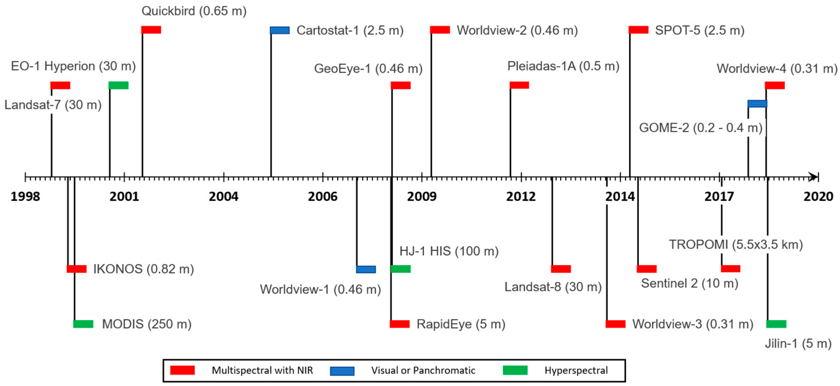
2. Remote Sensing Technologies in Agriculture: A Global Perspective on Past and Present Trends

To examine how RS technologies in the agricultural sector have evolved over the past 20 years (2000–2019), literature on the application of RS technologies in agriculture were compiled and reviewed. For this, a search was conducted using the Web of Science (Thomson Reuters) and Google Scholar. First, all articles with ‘agriculture’ and ‘remote sensing’ in the title were compiled, then the results were refined based on the types of sensor and platform in the title, abstract or keyword sections of the articles. Sensor types included visible (visual), multispectral, hyperspectral, thermal and microwave, and platforms included satellite, manned aircraft (airborne or aerial), and unmanned aerial vehicles (UAVs), unmanned aerial systems (UASs), or drones. During the search, only the papers published in peer-reviewed, scientific journals were considered. This resulted in a total of 3679 papers by type of platform and 3047 papers by sensors. In general, 64% and 26% of the total papers used satellite- and aerial-based imagery, respectively.

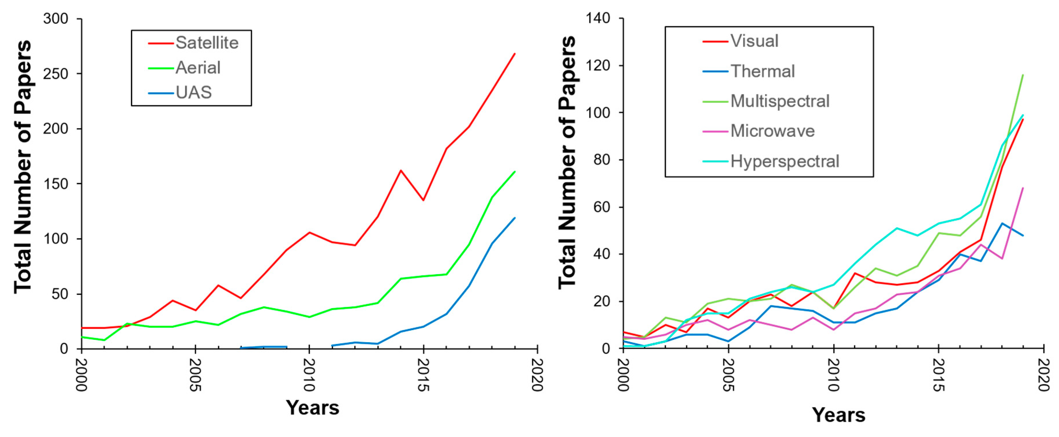
2.1. Temporal Trends

There has been an exponential growth in the number of studies focusing on the application of RS in agriculture over the 20-year period between 2000 and 2019. This suggests a substantial progress in relevant technology, including numerous sensors with unprecedented combinations of spatial, temporal, and spectral capacities of onboard satellites’ (e.g., Sentinels, Worldview) sensors, the advent of small UASs, and the development of cloud computing and machine learning techniques. Unlike satellite and UASs, studies based on manned aircraft-based RS have showed a slow increasing trend. Interest in UAS applications has increased, especially since 2015 (Figure 2). Just between 2015 and 2019, studies using satellite, UASs, and manned aircraft collected RS data for agricultural applications increased by 23%. In addition to the increased focus on UAS technologies in recent years, there has been a consistent increasing trend of satellite-based RS studies. This has been due in part to free access to a large volume of historic satellite images, such as Landsat and Sentinel, as well as the accessibility of powerful open-source data computing platforms such as Google Earth Engine (GEE) [14]. At present, the number of RS studies is approximately 20 times higher than it was in early 2000s, suggesting the availability of abundant resources to learn from. When we break down these studies by sensor types, we find that a majority of studies, particularly those after 2017, have focused on visual, multispectral, and hyperspectral sensors, as opposed to thermal and microwave.
Given that a hyperspectral sensor is comparatively expensive, and its data size is huge and thus involves extensive computations, it was bit surprising to see that a majority of studies have focused on hyperspectral sensors rather than visual and multispectral. While further investigations are needed to evaluate the potential reasons behind this, we found tendencies among studies, particularly those using satellite RS data, to not explicitly mention sensor type unless it was hyperspectral, thermal, or microwave. Visual or multispectral sensors are the most common form of sensor available across satellites. For example, prior works [15,16,17,18] have used Landsat satellite data in the visible and near IR region, but without explicitly stating the sensor type. This might have influenced not only the findings according to sensor type, but have also resulted in fewer number of studies when the search was limited to sensor type rather than platform.

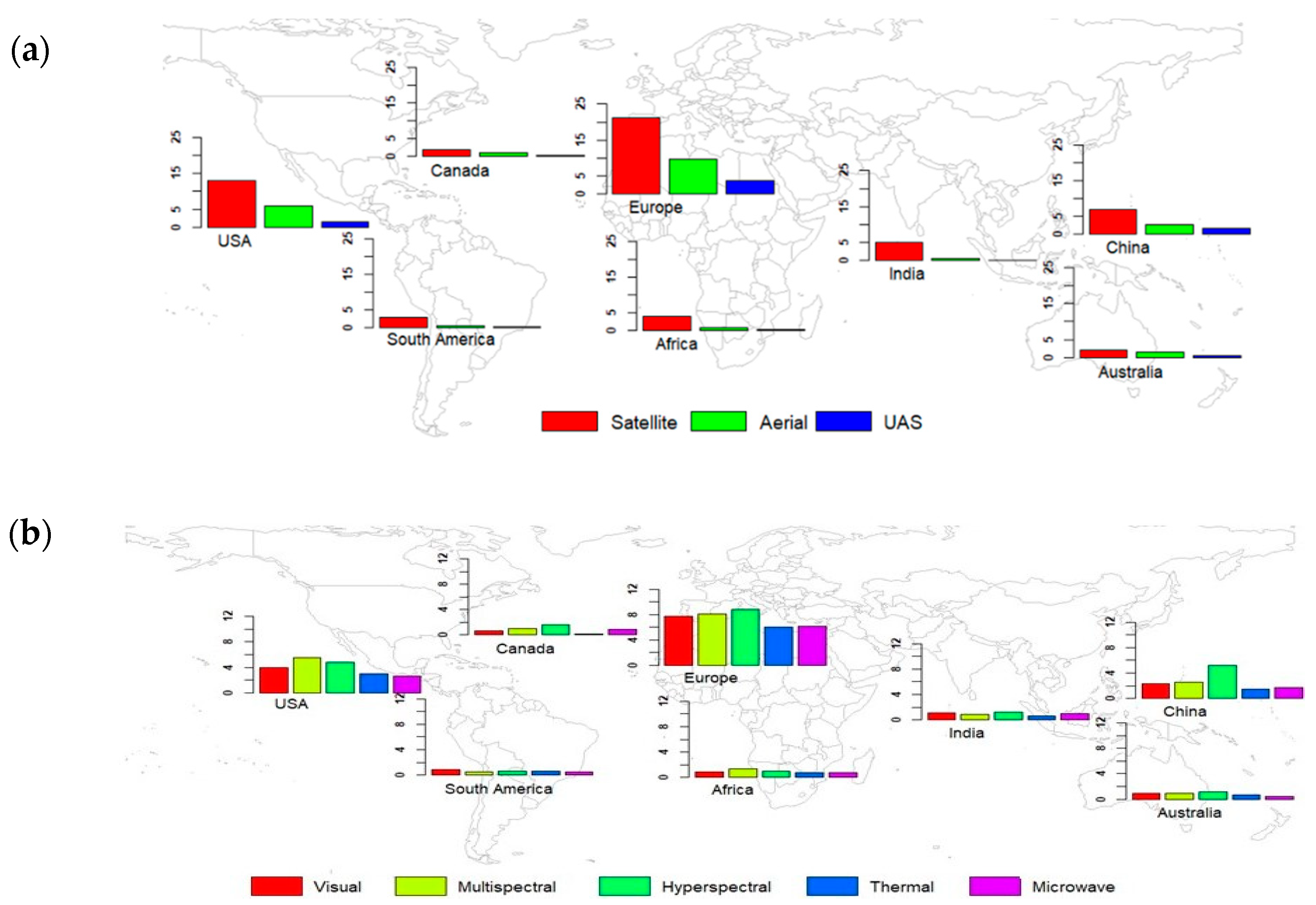
2.2. Geographical Distribution

When assessing these RS studies according to the region where they were conducted, Europe (34%) was in the forefront, followed by the United States (20%) and China (11%). Europe consistently had a large number of studies in all sensor and platform categories (Figure 3). Satellite-based studies were more prevalent than manned aircraft and UASs in these regions (Figure 3a). This is not surprising as the satellite-based RS technologies is a matured technology compared to aerial and UASs. There were relatively fewer manned aircraft- and UAS-based studies in India (0.6%), South America (0.9%), and Africa (1%), which could be a result of the comparatively limited resources and technical expertise on aircraft- and UAS-based technologies in these regions compared to the United States and Europe. A majority of studies in Europe, China, and Canada focused on hyperspectral sensors. For instance, in China, studies based on hyperspectral sensors were disproportionately higher than visual and multispectral sensors (i.e., 128% and 198%, respectively). However, in the United States and Africa, multispectral sensor-based studies were predominant (Figure 3b). At present, the most common form of earth-observing satellite data is obtained using multispectral sensors (Figure 1). However, most of the studies focused on satellite imagery have not explicitly mentioned the sensor/imagery type unless focused on hyperspectral satellite data, which involves relatively specialized and expensive hardware and software for data acquisition and processing. Thus, it is important to note that this interpretation might be biased.

3. Remote Sensing Applications in Precision Agriculture

3.1. Linking Remote Sensing Observations to Variables of Interest in Agriculture

In agriculture, some of the variables of interest include the characteristics of crops (e.g., morphological, biochemical, and physiological), soil properties (e.g., soil moisture, organic matter, pH, drainage), and topography (e.g., elevation, slope), and how they vary in space and time [19]. Since none of these traits can be measured directly through RS, they are often estimated by integrating spectral measurements with ground-truth data via empirical or mechanistic approaches or a combination of both [20]. For example, nitrogen (N) stress in crops has been linked to RS observations through empirical approaches by comparing spectral signatures in a target field with a reference spectral signature in a well-fertilized plot representative of the target field [21,22], or mechanistically by combining RS-based leaf area index and chlorophyll content with crop models [23]. Similarly, crop yield can be related to RS observations, but this involves the further consideration of other auxiliary variables such as weather (e.g., solar radiation, temperature, precipitation), vegetation conditions, and soil properties [24] via an empirical or mechanistic approaches [25]. Crop emergence mapping involves questions around geometry of crops and their leaf area indices, field conditions in the early part of the growing season, and spatial resolutions of the images [3,5].
Since empirical approaches directly relate inputs to outputs via pure statistical means, they are relatively simple, and to enhance the robustness of a model, there is a need for more data acquisition. On the other hand, mechanistic models focus on the cause and effect relationships between inputs and outputs by accounting for various biophysical processes involved [20]. They often rely on various assumptions, which may not always work. Prior studies [26] have discussed the pros and cons of these approaches at greater length. Although either mechanistic or empirical approaches can be used to characterize the same traits, one approach may be more suited over another to a given application.

3.2. Remote Sensing Observations to Variables of Interest in Agriculture: A Role of Resolution

The type of information accessible from RS that is most useful to support agricultural decision-making depends on the specific properties of sensors and their platforms, such as the positioning of satellite orbits, the positioning and orientation of UASs, and sensor characteristics. The most common properties of RS data are spatial, spectral, and temporal resolutions. While “spatial resolution” refers to the pixel size of an image that affects the ability to detect objects on the earth’s surface through imagery, “spectral resolution” refers to the number and size of spectral sampling intervals that affects the ability of a sensor to resolve features in the electromagnetic regions (EMRs). “Temporal resolution” refers to the frequency at which data are acquired. A sensor’s platform also indirectly influences illumination and atmospheric conditions during data acquisition, which can influence the signal-to-noise ratio. To be able to detect and quantify variables of interest, various artifacts inferred by the measurement conditions and sensor characteristics must be taken into account so that “error-free” inferences can be made.
For PA, it is usually desirable to acquire imagery of a higher spatial (less than decametric) and temporal (less than weekly) resolution. While high-resolution imagery is useful to applications such as weed detection, crop counting, and crop growth stage identification, frequent access to imagery at specific growth stages is useful to capture within-season variability in crop water and nutrient stresses. Similarly, an image capturing spectral signatures in several narrow spectral bands in EMRs (i.e., hyperspectral imagery) can help improve the characterization, identification, and classification of crop and soil properties that would otherwise be difficult to achieve by analyzing only a few broad spectral bands (i.e., multispectral). Furthermore, imagery capturing spectral signatures from thermal and microwave regions have been proven to be useful in capturing thermal anomalies in crops and soils (e.g., crop and soil water stress) over imagery capturing signatures in visual and near-infrared regions [27,28].
In the next section, we discuss the spatial and temporal resolutions of RS data used in prior studies, while evaluating the efficacy of RS to support decision-making in a series of management operations related to production agriculture such as pre-season planning, field preparation, planting, in-season monitoring, spraying for pest control, harvest, and post-harvest (Figure 4). We also focus on the accuracies reported by these studies.

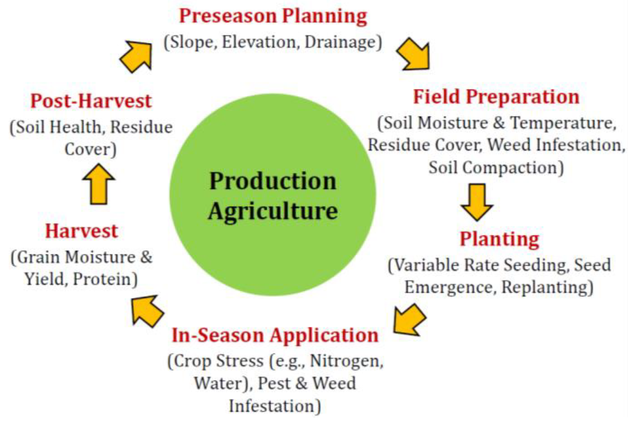
3.3. Remote Sensing Applications in Production Agriculture

3.3.1. Preseason Planning

Topography (elevation and slope) mapping: Preseason management decisions, such as timing of field operations, selection of crop type, and seeding rate for spring planting, are often dictated by topographic properties (e.g., slope, elevation, and aspect) of a field. Topography impacts hydrological balance, which influences soil conditions (e.g., moisture/temperature). Field topography can be derived based on digital elevation models (DEMs) delineated through the use of survey-grade global positioning system (GPS) equipment, GPS equipment mounted on farm equipment, or RS imagery. Survey-grade GPS equipment is more accurate, but is expensive and tedious to implement. Currently, pseudo-range GPS units mounted on field machinery are commonly used to provide on-the-go elevation data. These data are less accurate and thus are rarely used for topographic mapping [29,30]. Studies conducted by Yao and Clark (2000a, 2000b) revealed that using pseudo-range GPS units and taking measurements on the go can result in elevation biases of over 1 m.
Cost, time, and accuracy associated with topographic mapping can be reduced significantly through the use of RS data collected from satellites and aircrafts. The most common forms of creating DEMs include laser surveying, photogrammetry, and GPS [31]. Currently, satellite imagery-derived DEM data (e.g., 30 m × 30 m USGS Level 1) are the most commonly used DEM data in the United States. Although these data are accessible at no cost, it is of less use for PA as it has difficulty detecting in-field elevation variability due to its poor vertical accuracy (its root mean square error (RMSE) was reported to be 4.01 m [32]). Airborne Light Detection and Ranging (LiDAR)-derived DEM data are a better alternative [33,34] to satellite data. Vaze et al. [34] compared high- (1 m) resolution LiDAR DEM with field survey elevation points and observed only small differences. The accuracy of LiDAR DEM was significantly better than DEMs derived from contour maps and resampling (Table 1). Similarly, DEM derived from LiDAR showed higher accuracy even when the data were collected during leaf on conditions [33].
Recently, integration of photogrammetry and UAS-collected visual images has been found to be promising in deriving high-resolution DEMs for PA. For instance, Whitehead et al. (2014) conducted two UAS surveys over a stockpile in June and November using a visual camera onboard quadcopter, generating a 3.5-cm resolution DEM with relatively good accuracy. The root mean square error (RMSE) of vertical difference between the UAS-derived DEM and Global Navigation Satellite System (GNSS) points surveyed on the stockpile was less 0.11 m. Although photogrammetry techniques have been used to produce high-resolution DEMs [35,36] using UAS based imagery, to date, comprehensive evaluations of these DEMs for understanding terrain properties (soil type, soil wetness, drainage, and topographic variations within farm field) are lacking and need further investigation.
Subsurface tile drain mapping: Proper understanding of the spatial distribution of tile drainage systems in agricultural fields can support improved water management that can be used to boost crop productivity while reducing nutrient losses to streams. However, there is currently a limited understanding of the locations, extent, and density of existing tile drains (the terms “tile drains”, “drain lines”, and “tile lines” are used interchangeably), several of which were installed 50 or more years ago [37,38]. In most cases, information about old tile lines has either been lost or does not exist. Conventionally, drain lines have been located using heavy trenching equipment and handheld tile probes, which are time-consuming, extremely tedious, and inefficient for large-scale mapping. Recent studies that have used high-resolution imagery from UASs [37,38,39] (Table 2) have been in line with other studies [40,41] that concluded that RS technology has the potential to be a scalable, cost-effective, and accurate approach to detect and map drain lines.
Factors such as soil texture, organic matter, compactions due to farm machinery, and tillage can affect the reflectance of soil in VIS and near IR (NIR) wavelengths, which can add complexity to tile line detection [37,38,40,41]. However, some studies [42,43] have reported temperature differences between soil surfaces over a drain line and soil surfaces between adjacent drain lines, suggesting that thermal infrared (TIR) sensors can be exploited to address the limitations of VIS and NIR imagery in mapping tile lines [43,44,45]. Prior studies [41,46,47,48] have also suggested that the integration of satellite imagery, in-situ crop and soil data, and topographic variables with machine learning algorithms can be a practical alternative to estimating the intensities of tile-drained areas at a landscape scale. For instance, Gökkaya et al. [48] used decision tree classification (DTC) based on criteria such as land cover types, soil drainage classes, and surface slopes to map potential tile-drained areas in the Shatto Ditch watershed in Indiana.
Currently, tile drains are a large blind spot in our understanding of water routing and nutrient exports to water resources. While hydrologic and nutrient models such as such as SPARROW [49] and SWAT [50] have been widely used to assess nutrient exports, these models depend on an accurate understanding of river hydrography from datasets such as NHDPlus, which entirely neglect the dense networks of unmapped tile drains that supply water and nutrients to agricultural streams. These tile drain networks have potentially large implications for storm hydrology and nutrient fates at the watershed scale. Without adequate information on the distribution and connectivity of tile drain systems, it is difficult to ensure that hydrologic and nutrient export models are getting the “right” answers for the “right” reasons, particularly in watersheds and basins with extensive agricultural land use. Thus, further studies need to be conducted to determine the optimal field (i.e., soil and vegetative) conditions and quality of imagery (i.e., spatial and spectral resolution) necessary for detecting tile drainage patterns, as well as the advanced image processing techniques needed to support the automatic extraction of tile drain lines from imagery.

3.3.2. Field Preparation

Soil moisture and temperature mapping: Soil temperature and moisture status of a field is critical for management decisions related to planting, fertilizer application, and irrigation. Since soil moisture influences soil temperature, cool conditions during planting impose significant stresses on the emergence of warm season crops such as corn and soybean. Germination and emergence of corn are optimal when soil temperature is approximately 30–32 °C [52]. Similarly, fertilizers are typically applied when fields are not too wet to avoid the increased risk of nutrient loss and enhance crop nutrient uptake. Up to now, the majority of studies have focused on soil moisture estimation at a landscape scale using optical and thermal RS data by exploiting the physical relationship between land surface temperature and vegetative cover conditions using an approach referred to as “triangle” or “trapezoid”, or the land surface temperature-vegetation index [53,54,55,56,57,58]. Table 3 lists some of the prior studies that have reported correlation coefficients greater than 0.70 between coarse-resolution satellite-derived data and field-measured soil moisture data.
Compared to RS data acquired in the visible, NIR, and short-wave infrared bands, signals in the microwave region are less likely to be affected by interferences caused by atmospheric and cloud conditions, and thus have a greater potential to provide accurate soil moisture estimations. Currently, several satellites exist with active and passive microwave sensors for soil moisture monitoring, such as the soil moisture active passive (SMAP) and Sentinel-1 [56,59]. Some studies have used a combination of the synthetic aperture radar (SAR) from Sentinel 1 and optical RS data with machine learning techniques to downscale SMAP data. Despite developments in downscaling techniques, the spatial-temporal resolution of downscaled soil moisture data has insufficient spatial resolution for PA. Recent studies [60,61] have shown promising applications of machine learning techniques in estimating soil water content using high-resolution UAS-based multispectral and thermal imagery. Further efforts are needed to develop advanced downscaling techniques that combine data from multiple sources and provide soil moisture estimates at the finer spatial resolutions necessary for PA.
Soil compaction assessment: Soil compaction adversely impacts soil health by decreasing porosity, soil hydraulic conductivity, and nutrient availability, which results in reduced crop yield. Improved understanding of both the temporal and spatial extents of soil compaction in a field can help farmers to alleviate in-field compaction and related crop yield losses. Traditionally, a cone penetrometer is used to assess soil compaction as a function of penetration resistance per unit area—a method that is laborious, time-consuming, and yet incomplete due to the discrete nature of collected data. Currently, there are only a few studies that have used RS technologies to identify and quantify soil compaction. Kulkarni et al. [68] studied the response of soil compaction on canopy spectral reflectance and yields of cotton plants using hyperspectral data collected from the ground in Arkansas. The study demonstrated that the effects of soil compaction can be assessed through changes in the Green Normalized Difference Vegetation Index (GNDVI)—an index derived from green and NIR spectral bands of imagery. However, the relationship between the cone penetrometer and NIR data was found to be too weak to identify compacted soil areas [69] (Table 4).
Although some of these studies have provided a new perspective on soil compaction, knowledge on the spatial aspect of soil compaction during the year and its consequence on soil hydraulic properties are still lacking. Currently, there is no generally accepted method by which to measure mechanical properties in a way that helps estimate soil compaction in a field [70]. Since basic soil properties (e.g., texture, soil moisture, organic matter, and bulk density) play an important role in assessing soil functions and soil compaction [70,71], further investigation of RS-based assessments of soil properties and their integration with advanced machine learning algorithms to assess soil compaction deserves further research.

3.3.3. Planting

Crop emergence and density: The spatial and temporal variabilities of crop populations and their densities within a field can have a significant impact on grain and biomass yields as well as on harvesting logistics. The timely availability of such information can be used to influence replanting, as well as mid-season management decisions on variable-rate fertilizer, herbicide, and pesticide applications. Recent studies have demonstrated the utility of UASs for accurately detecting crops and quantifying their density in a field (Table 5). Recently, sophisticated computer vision algorithms and analytics have been developed to quantify crop features such as individual crop stands, sizes, and shapes (e.g., area, diameter, major axis length, minor axis length) using high spatial resolution images. These algorithms have shown that the accuracy to extract such features depends on the spatial resolution of images and crop growth stages [3,5]. For instance, images with a resolution ranging from 3.88 µm to 2.4 mm collected during early growth stages have been found to be useful in crop counting. Studies [3,5] have reported that UAS-based approaches can result in the highest accuracy if data are collected when crops have two to three leaves. Although recent efforts have focused on detecting and counting crop seedlings, as well as estimating plant spacing, very few studies if any have focused on the quantification of crop growth stages. Integration of crop growth stages with forecasted weather can help develop a precise supply forecasting capability for crop industries.

3.3.4. In-Season Crop Health Monitoring

Crops are subject to biotic (weeds, pest, insects, and pathogens) and abiotic (water, temperature, and nutrient) stresses during the growing season, which can influence quantity and quality of crop grains. For instance, the total yield loss due to pests (insects and disease) in soybean was more than 43.8 M bu in 2012 [74]. Traditional approaches for determining in-season crop stresses rely on crop scouts or laboratory experiments that are time-consuming and expensive if expanded to larger areas. The use of RS offers a timely and non-destructive approach for detecting, quantifying, and mapping crop related stresses, and is thus useful in guiding site-specific management decisions on nutrient and insecticide applications rather than whole-field applications.
Nitrogen stress monitoring: When a crop is in nitrogen stress, its chlorophyll content changes, resulting in changes in the optical properties of its leaves. Through analyses of crop spectral signatures, particularly in the VIS-NIR region of the Electromagnetic spectrum, prior studies [75,76,77,78] have shown the value of RS in monitoring N stress (Table 6). For example, Miao et al. [78] demonstrated that multispectral and hyperspectral data can explain about 71–86% and 73–88% variability of the ground-based chlorophyll measurements in corn plants at their multiple growth stages, respectively. However, studies have also shown that the efficacy of RS techniques for monitoring crop N stress can be limited by factors such as chlorophyll saturation, and atmospheric and soil interference [79]. While some studies have addressed some of these limitations by accounting for supplementary information regarding field condition (e.g., soil properties, elevation, management practices) in their empirical approach, others have recommended the integration of RS data with crop models that simulate crop growth and nutrient cycling [23,80]. Some studies [75,77] have used multiple vegetation indices (VIs) (e.g., NDVI, Renormalized Difference Vegetation Index (RDVI), Optimized Soil-Adjusted Vegetation Index (OSAVI), Transformed Chlorophyll Absorption in Reflectance Index (TCARI)) derived from a combination of multiple spectral bands in the EM spectrum, demonstrating that a combination of indices can improve N estimation by addressing the problem of saturated VI in high vegetation surfaces. Currently, most of the crop models are not spatially scalable due to need for field-specific measurements, which are often laborious and expensive to collect beyond a few experimental sites. Now that there is high accessibility to spatial and temporal resolution RS data, which has potential in addressing the data needs required by the crop models, further studies should focus on leveraging high-resolution RS with crop modeling to understand within-field variability in crop N stress and the potential agronomic benefits of variable-rate N applications [80].
Crop disease monitoring: Typically, pathogens tend to result in either loss of leaves and/or shoot area or changes in a leaf color due to a reduction in photosynthetic activity. These changes result in differences in spectral response in the VIS and NIR regions of the EM spectrum [81].
As such, prior studies [81,82] have been able to separate infected plants from healthy ones based on spectral responses in the VIS-NIR region. However, the early detection of crop disease is a challenge. The success of some of these studies has been limited to the later stages of infection, when crop damages are high and visible to naked eyes [9,83]. This delayed detection of crop disease could mean that it is too late to stop the infection for the current growing season. Recently, studies have shown the potential of thermal imagery for detecting crop diseases, as plants with disease tend to exhibit elevated temperatures compared to healthy plants, although pathogen symptoms are not visible [8,84,85] (Table 7). These studies have shown that the temperature of a leaf with disease is usually higher than in a healthy leaf, and thus a thermal sensor is more powerful in the early detection of diseases than VIS, multi-, and hyperspectral sensors. Additionally, recent studies [86,87] have demonstrated the strength of various machine learning methods (e.g., deep neural networks, decision trees) based on high-resolution VIS-NIR data for the detection and identification of plant pathogens at their early developmental stages. However, the success of these methods depends on a large database of images showing crop leaves with and without disease. Although some works have been dedicated to building databases such as PlantVillage [86,88], such a library has several limitations, including limited crop diseases and diseases specific to limited crop varieties. Further studies focused on the development of new databases, as well as the improvement of existing databases, are needed to enhance the application of powerful data-analytic tools for the detection and classification of crop diseases.
Weed identification and classification: Weeds usually cover only a small percentage of a crop field [95,96]. However, the common practice to control weeds has been to spray herbicides over the entire field, resulting in the waste of a significant amount of herbicides. To avoid this excessive and unnecessary use of herbicides, the concept of “patch spraying” was introduced in late 1970s and early 1980s [97,98,99,100], followed by technological developments to bring this concept to practice in the early 1990s. These developments started first with digital weed identification [101,102], followed by the integration of spray flow control algorithms and electronics to existing sprayers to turn the sprayer nozzles on and off, depending on the existence of weeds at a given GPS coordinate in the field [96,103,104]. Previously, satellite images were typically used to detect weeds [105]. However, due to the low-resolution satellite imagery, RS approaches to weed detection were not preferred until recent years, when high-resolution imagery became more accessible through UAS technology.
In addition to high-resolution (spatial and spectral) imagery, advanced image analytics (e.g., object-based image analysis (OBIA)) are ctitical to the accurate identification and classification of weeds [106,107,108] (Table 8). The optimal resolution of RS data required for weed mapping oftentimes depends on how different the crops are from weeds at certain growth stages. For instance, López-Granados et al. [106] reported accuracy in the range of 41–67% with lower-resolution (5.51 cm) imagery as compared to 86–92% with higher resolution (1.62 cm) imagery when UAS onboard visible and multispectral sensors were used to detect weed (Johnsongrass) populations in a corn field at corn’s early growth stage. Peña et al. [108] highlighted the importance of advanced analytics such as OBIA by combining the spectral, contextual, and morphological information from UAS-based multispectral imagery while classifying weed infestations in a corn field when plants were at the four- to six-leaf stage. Recently, deep learning approaches have exhibited promsing prospects in weed identification and classification, but the robustness of such approaches depend on a large amount of labelled samples for training, which can be labor-cost intensive [109,110]. Therefore, new learning networks (e.g., semi-supervised learning, generative adversarial networks (GAN)) should be considered as a part of future studies [110].

3.3.5. Harvest

Yield prediction: In the present day, some crop producers rely on yield-monitoring systems mounted on a combine during harvest to collect yield information. A yield monitor typically aggregates yield information from multiple crop rows at the time of harvest (e.g., a modern corn combine typically uses a 6-, 8-, 12-, or 16-row head [113]). The resolution of a yield map thus can be very coarse, and it becomes harder to detect crop yield by row [114]. Using emperical approaches, studies have demonstrated the potentials of RS imagery to generate high-resolution yield maps [115,116,117] to assess within-field yield variability at a field as well as a landscape scale [118], through which they can better understand the overall production potential of agricultural fields. These studies have used VIs derived from RS imagery and fit the data into machine learning algorithms to estimate crop yields with an R2 ranging from 0.57 to 0.94 (Table 9). These studies demonstrate that crop yield can be predicted with a high accuracy even through the use of visible imagery. Accuracy of yield prediction models, however, has ben shown to be dependent on crop growth stages. For instance, yield prediction models have been found to be more accurate when they are based off imagery collected during the mid-season rather than during earlier growth stages. However, the ability to predict crop yield earlier in the growing season is often crucial in minimizing potential crop yield losses.
To improve yield forecasting, prior studies [119,120] have proposed the idea of assimilating RS data into a mechanistic crop growth model based on seasonal weather forecasts and field management practices. Although this idea has been around for a long time, it is still underexplored. The increased accessiblity to more RS data and the development of advanced data analytics is likely to advance research towards the development of crop yield forecasting systems, much like what is done in weather forecasting.
Grain quality assessment: Grain quality is as important as grain quantity because of its impact on nutritional value, as well as the profitability of the production system. A better understanding of grain quality prior to harvest is important in order to support feedstock logistic and handling related decisions. Currently, there are very few studies focusing on a RS-based evaluation of grain quality. Some studies [43,121,122] have reported some success (R2 in the range of 0.64–0.85) in predicting grain protein using RS imagery (Table 10), and have highlighted the importance of the growth stage and spectral resolution in an accurate assessment of grain protein. For instance, Wang et al. [122] predicted wheat grain yield and protein content by analyzing and comparing multitemporal imagery from SPOT5 and HJ-1 CCD, and reported the highest accuracy (R2 = 0.64) when imagery was collected at the anthesis stage. These studies typically consider simpler cases of homogeneous landscapes. Since yield quality is highly dependent on genotype, further investigations into the use of RS for mapping crop genotypes and the role of genotypes in grain quality assessment are thus warranted.

3.3.6. Post-Harvest

Crop residue assessment: The smart management of crop residues is critical in order to improve soil quality and crop productivity while minimizing the operational challenges and negative environmental impacts of excessive residue [124]. Prior studies (Table 11) have shown the potential of RS for mapping the spatial distribution of crop residues in agricultural fields. For instance, Sharma et al. [125] used multispectral satellite imagery from Landsat ETM+ and Landsat OLI and observed that the spectral indices derived from VIS and NIR bands, such as the normalized difference tillage index (NDTI), could be helpful in differentiating the extent of residue cover related to various tillage practices for maize and soybean fields in South Central Nebraska. Galloza et al. [126] found hyperspectral-based indices performed better than multispectral-based indices. Similarly, hyperspectral TIR imagery from NASA’s Airborne Terrestrial Application Sensor (ATLAS) was found to better differentiate varying heat capacities between soil and residues in different residue management systems when compared to VIS and NIR imagery [127]. Due to poor spatial resolution of satellite imagery, these studies remained mainly at a landscape scale, and focused less on within-field variability in residue management. Currently, only a limited number of studies have focused on site-specific tillage practices for residue management, indicating the potential opportunites to employ UAS-based technology to monitor residue, which will help understand the role of residue management on soil-water-nutrient dynamics.

4. Remote Sensing for Precision Agriculture: Challenges, Limitations, and Opportunities

Currently, a majority of RS technologies have become accessible and affordable for the agricultural community due to the technological advancements in the acquisition systems, such as launches of new satellites (Figure 1), UAS and related regulations, robot platforms, and IoT, as well as through data storage and computation (e.g., Google Earth Engine, Amazon Cloud Computing) and advanced algorithms for deep learning techniques for data processing. However, the agricultural sector has not been able to fully embrace RS technologies from experimental to real-world settings until now [129,130]. Some of the factors behind this include: (1) a limited understanding on the efficacy of RS technologies by sensor and platform type, and the techno-economic benefits of such technologies, (2) the limited availability and training of RS-based decision-support tools, and (3) interoperability with data and tools from a variety of sources.
Efficacy of RS technologies: Recommendations for a suitable sensor for agricultural data collection are often guided by (1) the nature of problem (i.e., what to measure, why, when, and where), and (2) economics. Over the past decade, sensors capturing data in the VIS-NIR domain have been extensively exploited. A visible sensor provides useful information closer to the visible spectrum and can be limited to operations such as crop emergence, crop classification, and elevation mapping. On the other hand, sensors capturing information in the NIR and thermal regions are useful in detecting crop stresses that are invisble to naked eye. Hyperpectral sensors have the capability to detect and discriminate between specific features of objects with several hundreds of narrow spectral bands. The addition of these bands will increase data size, level of complexity, and hence the challenges associated with data storage and the related preprocessing (e.g., noise removal, smoothing) [131] and post processing (e.g., image segmentation, pattern recognition) [132,133]. To simplify hyperspectral data analysis, fast computers and large data storage are needed. Furthermore, hyperspectral sensors are sophisiticated and expensive. Thus, one must weigh the potential benefits of their application against the capital and operating costs of each sensor.
Econonomics of RS data collection: Currently, several platforms exist for RS data collection, and each of these platforms has its own pros and cons. Regarding the costs associated with satellite data, due to the recent proliferation of open-acces satellite data streams, medium resolution data (i.e., ≥10 m pixel size) from several satellite sensors (e.g., Landsat, Advanced Very High Resolution Radiometer (AVHRR), Advanced Spaceborne Thermal Emission and Reflection Radiameter (ASTER), Shuttle Radar Topography Mission (SRTM), the European Space Agency’s Sentinel satellite series) are available for free [134,135]. Other satellite data with a higher resolution (≤5 m) are available at some cost, with the cost varying depending on the resolution. For example, 5-m resolution images from RapidEye cost USD 1.28/km2, while 50 cm from GeoEye-1 costs around USD 25 /km2 [136]. Typically, a satellite mission covers a larger area, and thus the use of satellites for smaller projects can steeply increase costs [137]. For instance, a minimum order of imagery from high-resolution satellites (e.g., WorldView1/2, Pleides 1A/1B, QuickBird, and GeoEye-1) involves a geographic coverage of 100 km2 with a 5-km minimum order width for a new mission, and 25 km2 with a 2-km minimum order width if the data are archived. Additionally, most of the satellite platforms offering high spatial resolution data (WorldView-4, Plaides, Cartostat-1, QuickBird, GeoEye-1) are limited to the VIS-NIR region. Developments are still in progress to develop sensors that can provide high-resolution spatial, temporal, and spectral information beyond VIS-NIR [138,139,140]. Recently, new RS data types such as sun-induced fluorescence (SIF) [141,142] and L-band are being used for monitoring crop phenology, and the SWIR band for greenhouse gas monitoring [143]. Although promising, these data are available at very coarse resolutions (GOME-2 satellite at a 40-km spatial resolution, and TROPOMI onboard the Sentinel-5) [144] and are thus applicable only at a regional or global scale. Further, the use of satellite data is highly constrained by weather conditions (e.g., cloud and snow cover).
UAS platforms are an alternative solution by which to obtain high-frequency data at a localized scale that allows agricultural health monitoring at an individual plant level. However, UAS applications can be constrained by weather conditions (e.g., a maximum wind resistance of 10 m/s precipitation), limited spatial coverage due to limited battery life, and/or regulatory restrictions (flight operations within the line of sight), as well as the maximum payload, which limits the simultaneous use of multiple sensors [145]. Further, unlike satellite platforms [146], no standard procedure for the inflight calibration of UAS-borne sensors currently exists. Calibration of UAS-based images can be achieved through images acquired over calibration targets at specific times during the flight. As environmental conditions (e.g., illumination, cloud cover) may significantly vary throughout the flight, such calibration approaches may result in an inaccurate representation of spectral signals [147]. Regarding cost, the operation of UASs seems to be cost effective after an initial investment or purchase of instruments. However, it may not be economical if the area to be studied is of a larger size [148]. Currently, pricing for UAS and manned aircraft-based imagery in agriculture has been quoted around USD 7.4 to 12.4/ha (USD 3–5/acre) [136]. Manned aircraft can present a compromise between satellites and UASs by providing higher resolution (both spatial and temporal) imagery than a satellite and covering much larger areas than UASs; however, they require a person to operate, and thus involve a higher labor cost compared to UASs. As a result, despite increased interest in the use of UASs lately, most studies realted to agricultural RS have been limited to a low spatial and/or temporal coverage.
Availability of RS data, cloud computing, and machine learning: The RS community now has access to more data than ever. Petabyte-scale archives of RS data have become freely available from multiple US Government agencies (e.g., NASA, the US Geological Survey, and NOAA) [14,134], as well as the European Space Agency. However, there are several challenges in the use of big data, including (1) the volume and velocity of these data, which far exceed a standalone computer’s storage and computing limits, and (2) the various formats, spatiotemporal resolutions, and uncertainties of these data. All of these make real-time data processing more difficult, as well as the extraction of information and the automation of data analyses [149]. A wide variety of tools (e.g., TerraLib, Hadoop, GeoSpark, and GeoMesa) and platforms (Google Earth Engine, the NASA Earth Exchange, Amazon’s web services, or Microsoft’s Azure services) have emerged as new paradigms for addressing some of these challenges. Similarly, the development and use of deep learning algorithms is increasingly growing to either solve classification problems [86,150] or build complex empirical relationships to estimate crop variables using RS data [151,152]. However, the exploitation of cloud computing and deep learning algorithms to their full potential for agricultural applications is still in its infancy [149,153]. While recent efforts have been focused on cloud computing, some of the challenges that need to be addressed include (1) the optimization of database management systems in the cloud environment, (2) scalable real-time spatiotemporal mining methods that can address data complexities, and (3) enhancing protection of both sensitive data and users’ privacy [149,154].
With the increasing applications of machine learning algorithms to build relationships between inputs and outputs, there have been questions around the relevance of using and developing mechanistics models to capture underlying biogeophyiscal and chemical processes [120] for PA. Although powerful, machine learning algorithms ignore several underlying processes, and thus their performance can be constrained by the size and nature of a training dataset. Conversely, since the mechanistics models rely on underlying assumptions and relationship between variables, they can be extrapolated to other environmental conditions. Nevertheless, these two approaches are complementary, and the performance of machine learning can be enhanced through the integration of mechanistic models [155].
Decision support tools: While advanced sensing technologies, machine learning algorithms, and cloud computing infrastructures have enabled us to collect and process huge amounts of data in real-time environments, several practical considerations must remain. These tools call for visualizations in order to provide insights and actionable decisions by refining and reducing large complex datasets to simple graphs, maps, or table forms. Often, the benefits of RS or big data revolve around three steps. The first step is the exploration of “known unknowns” and “unknown unknowns” using search, extraction, and modeling techniques on a large volume of data from various sources. In the second step, the results from the first step are used to create various insights. Finally, these insights are disseminated via reports and interactive dashboards. Currently, various tools and techniques are available to support each of these steps, such as the R and python programing languages, and various software (Tableau, ArcGIS, QGIS, SAGA GIS, and GeoDa) and distributed information systems (e.g., webGIS, Google Earth Engine) [156,157]. Realizing the benefits of these tools, several public and private agencies have created webGIS-based crop and soil monitoring systems. For example, the United States Department of Agriculture has developed and put into operation a web service-based online vegetation-condition monitoring system known as VegScape, which is based on NASA MODIS satellite data [158] and CropScape, using on cropland data layer [159]. Similarly, Google Earth Engine is also currently being used to visualize and disseminate public data. However, application of tools like these offering special analytical and visualization capabilities is still limited. Similarly, significant efforts must be devoted to training the end-users of support decision tools. The development of user-friendly visualization systems for the easy and timely dissemination of RS-derived products and the training of end-users are likely to promote a wider adoption of PA.
Agricultural equipment companies and their role in the integration of RS technologies: There is a growing focus on the smart management of farm resources such as seeds, fertilizers, and pesticides by many countries around the world to reduce the environmental pollution associated with fertilizer and pesticide use. In response to this, several companies manufacturing machinery currently incorporate some sort of technology that supports the variable-rate application required for PA such as equipment guidance and automatic steering, in-field electronic sensors, and spatial data management systems. While the decision to collect RS data of optimal spatial, spectral and temporal resolutions often depends on the nature of problem at hand (as discussed in Section 3), it can also be influenced by farm machinery configurations to provide real-time assistance to carry out agile actions, especially in cases of sudden change in operational conditions (e.g., field or weather or nutrient or water or disease stress alert) [154]. Some of these relate to the concept of smart farming, which includes smart sensing and monitoring, smart analyses, and the planning and smart control of farm operations that utilize a cloud-based event management system [160]. Currently, modern agricultural equipment manufacturers have begun to use smart farming concepts in design of their equipment. For example, variable-rate N-management technologies such as Green Seeker, Crop Circle, and Yara N-Sensor use crop reflectance data to determine and apply spatially variable fertilizer rates in real-time [161]. Similarly, there are commercialized products for weed detection and subsequent site-specific weed management, such as the Sense and Decide from Blue River Technology (Sunnyvale, CA, USA), which was acquired by John Deere (Deere and Company, Miline, IL, USA), and the autonomous weed robot by ecoRobotix (ecoRobotix Ltd., Switzerland) and Deedfield Robotics (Renningen, Baden-Wurttemberg, Germany). These intelligent products are based on machine vision and image processing techniques [110]. Although these technologies are expected to promote PA practices, there are several challenges and bottlenecks in the utilization of smart farming technologies.
In addition to the challenges of handling large amounts of data from multiple sensors within the agricultural equipment, there are issues of interoperability between data (i.e., lack of unified data formats) and property solutions from agricutlural industries, as well as data protection/ownership. These issues have to be overcome to achieve a wide expansion and adoption of effective, efficient, and cheap technological solutions for farming. Similarly, although prior studies have shown the suitability of RS technologies in reducing farm resources and promoting crop productivity—and hence increasing profitability—additional research and development needs to be done to quantify the tangible and intangible benfits of PA technologies [129,130,162,163].

5. Conclusions

In conclusion, a review of prior works provided an extensive overview of the trend of RS studies in agriculture temporally and spatially around the world, detailing the various applications of RS at different stages of crop production. We found that a majority of these studies were based on satellite technologies conducted in developed countries/regions, mainly Europe followed by the United States and China. Currently, studies focused on UAS technologies make up 16.3% of the RS studies in agriculture between 2015 and 2019. Of the total RS studies in agriculture, a large percentage have focused on hyperspectral sensors, followed by multispectral and visual sensors. Our review of prior studies showed the potential of RS technologies to support management decisions at various stages of production agriculture, ranging from field preparation to in-season crop health monitoring to harvest. The main findings of the review of prior RS works focused on various phases of production agriculture are summarized as follows.
  • LiDAR-derived data can offer an accurate representation of topography, but recent photogrammetry approaches using visual images collected by UASs have been found promising for within-field variability in topography.
  • High-resolution thermal imagery has been found useful for detecting temperature differences between soil surfaces over a drain line and between drain lines, and can help detect sub-surface tile drain lines—a significant advantage over VIS and multispectral imagery.
  • A majority of prior RS studies on soil moisture have focused on medium- to coarse-resolution multispectral, thermal, and hyperspectral imagery and were conducted at larger agricultural landscape scales than a field level. With advancements in data analytics and UAS technology, a recent focus has been placed on examining the downscaling of satellite-based soil moisture estimation, as well as applications of UAS for high-resolution soil moisture mapping.
  • Unlike other aspects of production agriculture, the applications of RS for soil compaction and grain quality monitoring have been less explored and deserve further investigation.
  • Advanced comptuer vision algorithms and analytics on high-resolution visual imagery have provided opportunities to quantify (1) crop emergence and spacing, as well as important crop features, and (2) the identification and classification of weeds and crop diseases.
  • Most of the existing RS studies focused on nitrogen stress and yield assessment have been based on empirical approaches. Further studies should focus on leveraging RS data with crop modeling to understand and forecast crop dynamics, including N stresses and yields.
  • Thermal RS offer advanatages over visual and multispectral RS in the early detection of crop disease.
  • Prior RS works have focused mainly on assessing crop residues at a landscape scale. Site-specific residue management decsions can benefit from high-resolution RS data.
Remote sensing technologies have evolved over the years, and the present-day agricultural sector has a multitude of options in terms of both platforms (satellite to manned aircraft to UAS) and sensors (e.g., visible, multispectral, hyperspectral, thermal) by which to collect a variety of agricultural data. With the availability of such sensors and platforms, it is important for the agricultural community to develop a better understanding of the opportunities and limitations of each technology to help ensure that the value is derived from data while minimizing the cost and technical hurdles of data collection and utilization. By using RS data, the agricultural community can identify and quantify the health of agricultural systems, helping them to make management decisions that can increase farm profits while lowering agriculture-driven environmental problems.

Author Contributions

Conceptualization, S.K. and J.P.F.; methodology, S.K. and K.K.; formal analysis, S.K. and K.K.; writing—original draft preparation, S.K. and K.K.; writing—review and editing, S.K., K.K., J.P.F., S.S. and E.O.; project administration, S.K. and J.F.; funding acquisition, S.K. and J.P.F. All authors have read and agreed to the published version of the manuscript.

Funding

This work was supported in parts by funds from Ohio Agricultural Research and Development Center (OARDC) (SEEDS: the OARDC Research Enhancement Competitive Grants Program) and Hatch Project #NC1195.

Conflicts of Interest

The authors declare no conflict of interest. The funders had no role in the design of the study; in collection, analysis, or interpretation of data; in writing the manuscript; or in the decision to publish the results.

References

  1. Bauer, M.E.; Cipra, J.E. Identification of agricultural crops by computer processing of ERTS-MSS data. LARS Tech. Rep. Pap. 1973, 20, 205–212. [Google Scholar]
  2. Yu, Z.; Cao, Z.; Wu, X.; Bai, X.; Qin, Y.; Zhuo, W.; Xiao, Y.; Zhang, X.; Xue, H. Automatic image-based detection technology for two critical growth stages of maize: Emergence and three-leaf stage. Agric. For. Meteorol. 2013, 174, 65–84. [Google Scholar] [CrossRef]
  3. Jin, X.; Liu, S.; Baret, F.; Hemerlé, M.; Comar, A. Estimates of plant density of wheat crops at emergence from very low altitude UAV imagery. Remote Sens. Environ. 2017, 198, 105–114. [Google Scholar] [CrossRef] [Green Version]
  4. Gnädinger, F.; Schmidhalter, U. Digital counts of maize plants by Unmanned Aerial Vehicles (UAVs). Remote Sens. 2017, 9, 544. [Google Scholar] [CrossRef] [Green Version]
  5. Varela, S.; Dhodda, P.R.; Hsu, W.H.; Prasad, P.V.V.; Assefa, Y.; Peralta, N.R.; Griffin, T.; Sharda, A.; Ferguson, A.; Ciampitti, I.A. Early-season stand count determination in Corn via integration of imagery from unmanned aerial systems (UAS) and supervised learning techniques. Remote Sens. 2018, 10, 343. [Google Scholar] [CrossRef] [Green Version]
  6. Fernandez-Ordoñez, Y.M.; Soria-Ruiz, J. Maize crop yield estimation with remote sensing and empirical models. In Proceedings of the 2017 IEEE International Geoscience and Remote Sensing Symposium (IGARSS), Fort Worth, TX, USA, 23–28 July 2017; pp. 3035–3038. [Google Scholar] [CrossRef]
  7. Yao, X.; Wang, N.; Liu, Y.; Cheng, T.; Tian, Y.; Chen, Q.; Zhu, Y. Estimation of wheat LAI at middle to high levels using unmanned aerial vehicle narrowband multispectral imagery. Remote Sens. 2017, 9, 1304. [Google Scholar] [CrossRef] [Green Version]
  8. Calderón, R.; Navas-Cortés, J.A.; Lucena, C.; Zarco-Tejada, P.J. High-resolution airborne hyperspectral and thermal imagery for early detection of Verticillium wilt of olive using fluorescence, temperature and narrow-band spectral indices. Remote Sens. Environ. 2013, 139, 231–245. [Google Scholar] [CrossRef]
  9. Khanal, S.; Fulton, J.; Shearer, S. An overview of current and potential applications of thermal remote sensing in precision agriculture. Comput. Electron. Agric. 2017, 139, 22–32. [Google Scholar] [CrossRef]
  10. Hassan-Esfahani, L.; Torres-Rua, A.; Jensen, A.; Mckee, M. Spatial Root Zone Soil Water Content Estimation in Agricultural Lands Using Bayesian-Based Artificial Neural Networks and High- Resolution Visual, NIR, and Thermal Imagery. Irrig. Drain. 2017, 66, 273–288. [Google Scholar] [CrossRef]
  11. Park, S.; Ryu, D.; Fuentes, S.; Chung, H.; Hernández-Montes, E.; O’Connell, M. Adaptive estimation of crop water stress in nectarine and peach orchards using high-resolution imagery from an unmanned aerial vehicle (UAV). Remote Sens. 2017, 9, 828. [Google Scholar] [CrossRef] [Green Version]
  12. Betbeder, J.; Fieuzal, R.; Baup, F. Assimilation of LAI and Dry Biomass Data From Optical and SAR Images Into an Agro-Meteorological Model to Estimate Soybean Yield. IEEE J. Sel. Top. Appl. Earth Obs. Remote Sens. 2016, 9, 2540–2553. [Google Scholar] [CrossRef]
  13. Lopez-Sanchez, J.; Vicente-Guijalba, F.; Erten, E.; Campos-Taberner, M.; Garcia-Haro, F. Retrieval of vegetation height in rice fields using polarimetric SAR interferometry with TanDEM-X data. Remote Sens. Environ. 2017, 192, 30–44. [Google Scholar] [CrossRef] [Green Version]
  14. Gorelick, N.; Hancher, M.; Dixon, M.; Ilyushchenko, S.; Thau, D.; Moore, R. Google Earth Engine: Planetary-scale geospatial analysis for everyone. Remote Sens. Environ. 2017, 202, 18–27. [Google Scholar] [CrossRef]
  15. Farg, E.; Ramadan, M.N.; Arafat, S.M. Classification of some strategic crops in Egypt using multi remotely sensing sensors and time series analysis. Egypt. J. Remote Sens. Space Sci. 2019, 22, 263–270. [Google Scholar] [CrossRef]
  16. Habibie, M.I.; Noguchi, R.; Shusuke, M.; Ahamed, T. Land Suitability Analysis for Maize Production in Indonesia Using Satellite Remote Sensing and GIS-Based Multicriteria Decision Support System. GeoJournal 2019, 5. [Google Scholar] [CrossRef]
  17. Tasumi, M. Estimating evapotranspiration using METRIC model and Landsat data for better understandings of regional hydrology in the western Urmia Lake Basin. Agric. Water Manag. 2019, 226, 105805. [Google Scholar] [CrossRef]
  18. Xie, Z.; Phinn, S.R.; Game, E.T.; Pannell, D.J.; Hobbs, R.J.; Briggs, P.R.; McDonald-Madden, E. Using Landsat observations (1988–2017) and Google Earth Engine to detect vegetation cover changes in rangelands—A first step towards identifying degraded lands for conservation. Remote Sens. Environ. 2019, 232, 111317. [Google Scholar] [CrossRef]
  19. Nock, C.A.; Vogt, R.J.; Beisner, B.E. Functional Traits. eLS 2016, 1–8. [Google Scholar] [CrossRef]
  20. Baker, R.E.; Peña, J.M.; Jayamohan, J.; Jérusalem, A. Mechanistic models versus machine learning, a fight worth fighting for the biological community? Biol. Lett. 2018, 14, 1–4. [Google Scholar] [CrossRef]
  21. Raun, W.R.; Solie, J.B.; Stone, M.L.; Martin, K.L.; Freeman, K.W.; Mullen, R.W.; Zhang, H.; Schepers, J.S.; Johnson, G.V. Optical sensor-based algorithm for crop nitrogen fertilization. Commun. Soil Sci. Plant Anal. 2005, 36, 2759–2781. [Google Scholar] [CrossRef] [Green Version]
  22. Bushong, J.T.; Mullock, J.L.; Miller, E.C.; Raun, W.R.; Brian Arnall, D. Evaluation of mid-season sensor based nitrogen fertilizer recommendations for winter wheat using different estimates of yield potential. Precis. Agric. 2016, 17, 470–487. [Google Scholar] [CrossRef]
  23. Baret, F.; Houlès, V.; Guérif, M. Quantification of plant stress using remote sensing observations and crop models: The case of nitrogen management. J. Exp. Bot. 2007, 58, 869–880. [Google Scholar] [CrossRef] [PubMed] [Green Version]
  24. Prasad, A.K.; Chai, L.; Singh, R.P.; Kafatos, M. Crop yield estimation model for Iowa using remote sensing and surface parameters. Int. J. Appl. Earth Obs. Geoinf. 2006, 8, 26–33. [Google Scholar] [CrossRef]
  25. Bustos-Korts, D.; Boer, M.P.; Malosetti, M.; Chapman, S.; Chenu, K.; Zheng, B.; van Eeuwijk, F.A. Combining Crop Growth Modeling and Statistical Genetic Modeling to Evaluate Phenotyping Strategies. Front. Plant Sci. 2019, 10, 1491. [Google Scholar] [CrossRef]
  26. Estes, L.D.; Bradley, B.A.; Beukes, H.; Hole, D.G.; Lau, M.; Oppenheimer, M.G.; Schulze, R.; Tadross, M.A.; Turner, W.R. Comparing mechanistic and empirical model projections of crop suitability and productivity: Implications for ecological forecasting. Glob. Ecol. Biogeogr. 2013, 22, 1007–1018. [Google Scholar] [CrossRef]
  27. Hong, M.; Bremer, D.J.; Merwe, D. Thermal Imaging Detects Early Drought Stress in Turfgrass Utilizing Small Unmanned Aircraft Systems. Agrosyst. Geosci. Environ. 2019, 2, 1–9. [Google Scholar] [CrossRef] [Green Version]
  28. Möller, M.; Alchanatis, V.; Cohen, Y.; Meron, M.; Tsipris, J.; Naor, A.; Ostrovsky, V.; Sprintsin, M.; Cohen, S. Use of thermal and visible imagery for estimating crop water status of irrigated grapevine. J. Exp. Bot. 2007, 58, 827–838. [Google Scholar] [CrossRef] [Green Version]
  29. Renschler, C.S.; Flanagan, D.C.; Engel, B.A.; Kramer, L.A.; Sudduth, K.A. Site–specific decision–making based on RTK GPS survey and six alternative elevation data sources: Watershed topography and delineation. Trans. ASABE 2002, 45, 1883–1895. [Google Scholar] [CrossRef] [Green Version]
  30. Renschler, C.S.; Flanagan, D.C. Site-specific decision-making based on RTK GPS survey and six alternative elevation data sources: Soil erosion predictions. Trans. ASABE 2008, 51, 413–424. [Google Scholar] [CrossRef]
  31. Wang, X.; Holland, D.M.; Gudmundsson, G.H. Accurate coastal DEM generation by merging ASTER GDEM and ICESat/GLAS data over Mertz Glacier, Antarctica. Remote Sens. Environ. 2018, 206, 218–230. [Google Scholar] [CrossRef]
  32. Gesch, D.B.; Oimoen, M.J.; Evans, G.A. Accuracy Assessment of the U.S. Geological Survey National Elevation Dataset, and Comparison with Other Large-Area Elevation Datasets-SRTM and ASTER. US Geol. Surv. Open-File Rep. 2014, 1008, 18. [Google Scholar] [CrossRef]
  33. Hodgson, M.E.; Jensen, J.R.; Schmidt, L.; Schill, S.; Davis, B. An evaluation of LIDAR- and IFSAR-derived digital elevation models in leaf-on conditions with USGS Level 1 and Level 2 DEMs. Remote Sens. Environ. 2003, 84, 295–308. [Google Scholar] [CrossRef]
  34. Vaze, J.; Teng, J.; Spencer, G. Impact of DEM accuracy and resolution on topographic indices. Environ. Model. Softw. 2010, 25, 1086–1098. [Google Scholar] [CrossRef]
  35. Neugirg, F.; Stark, M.; Kaiser, A.; Vlacilova, M.; Della Seta, M.; Vergari, F.; Schmidt, J.; Becht, M.; Haas, F. Erosion processes in calanchi in the Upper Orcia Valley, Southern Tuscany, Italy based on multitemporal high-resolution terrestrial LiDAR and UAV surveys. Geomorphology 2016, 269, 8–22. [Google Scholar] [CrossRef]
  36. Whitehead, K.; Hugenholtz, C.H. Remote sensing of the environment with small unmanned aircraft systems (UASs), part 1: A review of progress and challenges. J. Unmanned Veh. Syst. 2014, 02, 69–85. [Google Scholar] [CrossRef]
  37. Allred, B.; Eash, N.; Freeland, R.; Martinez, L.; Wishart, D.B. Effective and efficient agricultural drainage pipe mapping with UAS thermal infrared imagery: A case study. Agric. Water Manag. 2018, 197, 132–137. [Google Scholar] [CrossRef]
  38. Allred, B.; Martinez, L.; Fessehazion, M.K.; Rouse, G.; Williamson, T.N.; Wishart, D.; Koganti, T.; Featheringill, R. Overall results and key findings on the use of UAV visible-color, multispectral, and thermal infrared imagery to map agricultural drainage pipes. Agric. Water Manag. 2020, 232, 106036. [Google Scholar] [CrossRef]
  39. Williamson, T.N.; Dobrowolski, E.G.; Meyer, S.M.; Frey, J.W.; Allred, B.J. Delineation of tile-drain networks using thermal and multispectral imagery—Implications for water quantity and quality differences from paired edge-of-field sites. J. Soil Water Conserv. 2018, 74, 1–11. [Google Scholar] [CrossRef] [Green Version]
  40. Verma, A.K.; Cooke, R.A.; Wendte, L. Mapping Subsurface Drainage Systems with Color Infrared Aerial Photographs; Department of Agricultural Engineering, University of Illinois: Urbana, IL, USA; Champaign, IL, USA, 1996. [Google Scholar]
  41. Naz, B.S.; Ale, S.; Bowling, L.C. Detecting subsurface drainage systems and estimating drain spacing in intensively managed agricultural landscapes. Agric. Water Manag. 2009, 96, 627–637. [Google Scholar] [CrossRef]
  42. Smedema, L.K.; Vlotman, W.F.; Rycroft, D. Modern Land Drainage: Planning, Design and Management of Agricultural Drainage Systems; CRC Press: Boca Raton, FL, USA, 2004. [Google Scholar]
  43. Jensen, J. Remote sensing of soils, minerals, and geomorphology. In Remote Sensing of the Environment; Pearson Education: London, UK, 2007; pp. 457–524. [Google Scholar]
  44. Mira, M.; Valor, E.; Boluda, R.; Caselles, V.; Coll, C. Influence of the soil moisture effect on the thermal infrared emissivity. Tethys 2007, 4, 3–9. [Google Scholar] [CrossRef] [Green Version]
  45. Abdel-Hardy, M.; Abdel-Hafez, M.; Karbs, H. Subsurface Drainage Mapping by Airborne Infrared Imagery Techniques. Proc. Okla. Acad. Sci. 1970, 50, 10–18. [Google Scholar]
  46. Sugg, Z. Assessing US Farm Drainage: Can GIS Lead to Better Estimates of Subsurface Drainage Extent; World Resources Institute: Washington, DC, USA, 2007; p. 20002. [Google Scholar]
  47. Thayn, J.B.; Campbell, M.; Deloriea, T. Mapping Tile-Drained Agricultural Lands; Institute Geospatial Analsyis Mapping (GEOMAP); Illinois State University: Normal, IL, USA, 2011. [Google Scholar]
  48. Gökkaya, K.; Budhathoki, M.; Christopher, S.F.; Hanrahan, B.R.; Tank, J.L. Subsurface tile drained area detection using GIS and remote sensing in an agricultural watershed. Ecol. Eng. 2017, 108, 370–379. [Google Scholar] [CrossRef]
  49. Schwarz, G.E.; Hoos, A.B.; Alexander, R.B.; Smith, R.A. The SPARROW surface water-quality model: Theory, application and user documentation. US Geol. Surv. Tech. Methods Rep. B 2006, 6, 248. [Google Scholar]
  50. Koch, S.; Bauwe, A.; Lennartz, B. Application of the SWAT model for a tile-drained lowland catchment in North-Eastern Germany on subbasin scale. Water Resour. Manag. 2013, 27, 791–805. [Google Scholar] [CrossRef]
  51. Naz, B.S.; Bowling, L.C. Automated identification of tile lines from remotely sensed data. Trans. ASABE 2008, 51, 1937–1950. [Google Scholar] [CrossRef]
  52. Pioneer. Soil Temperature and Corn Emergence; Pioneer: Banora Point, Australia, 2019. [Google Scholar]
  53. Zhang, K.; Kimball, J.S.; Running, S.W. A review of remote sensing based actual evapotranspiration estimation. WIREs Water 2016, 3, 834–853. [Google Scholar] [CrossRef]
  54. Carlson, T. An Overview of the ‘Triangle Method’ for Estimating Surface Evapotranspiration and Soil Moisture from Satellite Imagery. Sensors 2007, 7, 1612–1629. [Google Scholar] [CrossRef] [Green Version]
  55. Zhu, W.; Jia, S.; Lv, A. A Universal Ts-VI Triangle Method for the Continuous Retrieval of Evaporative Fraction From MODIS Products. J. Geophys. Res. Atmos. 2017, 122, 10206–10227. [Google Scholar] [CrossRef]
  56. Babaeian, E.; Sadeghi, M.; Franz, T.E.; Jones, S.; Tuller, M. Mapping soil moisture with the OPtical TRApezoid Model (OPTRAM) based on long-term MODIS observations. Remote Sens. Environ. 2018, 211, 425–440. [Google Scholar] [CrossRef]
  57. Verstraeten, W.W.; Veroustraete, F.; Feyen, J. Assessment of Evapotranspiration and Soil Moisture Content Across Different Scales of Observation. Sensors 2008, 8, 70–117. [Google Scholar] [CrossRef] [Green Version]
  58. Zhang, D.; Zhou, G. Estimation of Soil Moisture from Optical and Thermal Remote Sensing: A Review. Sensors 2016, 16, 1308. [Google Scholar] [CrossRef] [PubMed] [Green Version]
  59. Chen, S.; She, D.; Zhang, L.; Guo, M.; Liu, X. Spatial downscaling methods of soil moisture based on multisource remote sensing data and its application. Water 2019, 11, 1401. [Google Scholar] [CrossRef] [Green Version]
  60. Hassan-Esfahani, L.; Torres-Rua, A.; Jensen, A.; McKee, M. Assessment of surface soil moisture using high-resolution multi-spectral imagery and artificial neural networks. Remote Sens. 2015, 7, 2627–2646. [Google Scholar] [CrossRef] [Green Version]
  61. Aboutalebi, M.; Allen, N.; Torres-Rua, A.F.; McKee, M.; Coopmans, C. Estimation of soil moisture at different soil levels using machine learning techniques and unmanned aerial vehicle (UAV) multispectral imagery. Auton. Air Gr. Sens. Syst. Agric. Optim. Phenotyping IV 2019, 11008, 110080S. [Google Scholar]
  62. Gao, Z.; Xu, X.; Wang, J.; Yang, H.; Huang, W.; Feng, H. A method of estimating soil moisture based on the linear decomposition of mixture pixels. Math. Comput. Model. 2013, 58, 606–613. [Google Scholar] [CrossRef]
  63. Soliman, A.; Heck, R.J.; Brenning, A.; Brown, R.; Miller, S. Remote sensing of soil moisture in vineyards using airborne and ground-based thermal inertia data. Remote Sens. 2013, 5, 3729–3748. [Google Scholar] [CrossRef] [Green Version]
  64. Kalieta, A.L.; Tian, L.F.; Hirschi, M.C. Relationship Between Soil Moisture Content and Soil Surface Reflectance. Trans. ASAE 2005, 48, 1979–1986. [Google Scholar] [CrossRef] [Green Version]
  65. Peng, J.; Shen, H.; He, S.W.; Wu, J.S. Soil moisture retrieving using hyperspectral data with the application of wavelet analysis. Environ. Earth Sci. 2013, 69, 279–288. [Google Scholar] [CrossRef]
  66. Mobasheri, M.R.; Amani, M. Soil moisture content assessment based on Landsat 8 red, near-infrared, and thermal channels. J. Appl. Remote Sens. 2016, 10, 026011. [Google Scholar] [CrossRef]
  67. Amani, M.; Parsian, S.; MirMazloumi, S.M.; Aieneh, O. Two new soil moisture indices based on the NIR-red triangle space of Landsat-8 data. Int. J. Appl. Earth Obs. Geoinf. 2016, 50, 176–186. [Google Scholar] [CrossRef]
  68. Kulkarni, S.S.; Bajwa, S.G.; Huitink, G. Investigation of the effects of soil compaction in cotton. Am. Soc. Agric. Biol. Eng. 2010, 53, 667–674. [Google Scholar] [CrossRef]
  69. Wells, L.G.; Stombaugh, T.S.; Shearer, S.A. Application and Assessment of Precision Deep Tillage; American Society of Agricultural and Biological Engineers: St. Joseph, MI, USA, 2013; Volume 1. [Google Scholar]
  70. Alaoui, A.; Diserens, E. Mapping soil compaction—A review. Curr. Opin. Environ. Sci. Health 2018, 5, 60–66. [Google Scholar] [CrossRef]
  71. Troldborg, M.; Aalders, I.; Towers, W.; Hallett, P.D.; McKenzie, B.M.; Bengough, A.G.; Lilly, A.; Ball, B.C.; Hough, R.L. Application of Bayesian Belief Networks to quantify and map areas at risk to soil threats: Using soil compaction as an example. Soil Tillage Res. 2013, 132, 56–68. [Google Scholar] [CrossRef]
  72. Li, B.; Xu, X.; Han, J.; Zhang, L.; Bian, C.; Jin, L.; Liu, J. The estimation of crop emergence in potatoes by UAV RGB imagery. Plant Methods 2019, 15, 1–14. [Google Scholar] [CrossRef] [PubMed] [Green Version]
  73. Zhao, B.; Zhang, J.; Yang, C.; Zhou, G.; Ding, Y.; Shi, Y.; Zhang, D.; Xie, J.; Liao, Q. Rapeseed seedling stand counting and seeding performance evaluation at two early growth stages based on unmanned aerial vehicle imagery. Front. Plant Sci. 2018, 9, 1–17. [Google Scholar] [CrossRef] [PubMed]
  74. USDA NASS. United States Department of Agriculture—National Agricultural Statistics Service. 2012 ARMS-Soybean Industry Highlights; 2014; pp. 1–4. Available online: https://www.nass.usda.gov/Surveys/Guide_to_NASS_Surveys/Ag_Resource_Management/ARMS_Soybeans_Factsheet/ARMS_2013_Soybeans.pdf (accessed on 4 October 2020).
  75. Cilia, C.; Panigada, C.; Rossini, M.; Meroni, M.; Busetto, L.; Amaducci, S.; Boschetti, M.; Picchi, V.; Colombo, R. Nitrogen status assessment for variable rate fertilization in maize through hyperspectral imagery. Remote Sens. 2014, 6, 6549–6565. [Google Scholar] [CrossRef] [Green Version]
  76. Khanal, S.; Fulton, J.; Douridas, N.; Klopfenstein, A.; Shearer, S. Integrating aerial images for in-season nitrogen management in a corn field. Comput. Electron. Agric. 2018, 148, 121–131. [Google Scholar] [CrossRef]
  77. Gabriel, J.L.; Zarco-Tejada, P.J.; López-Herrera, P.J.; Pérez-Martín, E.; Alonso-Ayuso, M.; Quemada, M. Airborne and ground level sensors for monitoring nitrogen status in a maize crop. Biosyst. Eng. 2017, 160, 124–133. [Google Scholar] [CrossRef]
  78. Miao, Y.; Mulla, D.J.; Randall, G.W.; Vetsch, J.A.; Vintila, R. Combining chlorophyll meter readings and high spatial resolution remote sensing images for in-season site-specific nitrogen management of corn. Precis. Agric. 2009, 10, 45–62. [Google Scholar] [CrossRef]
  79. Muñoz-Huerta, R.F.; Guevara-Gonzalez, R.G.; Contreras-Medina, L.M.; Torres-Pacheco, I.; Prado-Olivarez, J.; Ocampo-Velazquez, R.V. A Review of Methods for Sensing the Nitrogen Status in Plants: Advantages, Disadvantages and Recent Advances. Sensors 2013, 13, 10823–10843. [Google Scholar] [CrossRef]
  80. Jin, Z.; Archontoulis, S.V.; Lobell, D.B. How much will precision nitrogen management pay off? An evaluation based on simulating thousands of corn fields over the US Corn-Belt. Field Crop. Res. 2019, 240, 12–22. [Google Scholar] [CrossRef]
  81. West, J.S.; Bravo, C.; Oberti, R.; Lemaire, D.; Moshou, D.; Alastair, M.H. The Potential of Optical Canopy Measurement for Targeted Control of Field Crop Diseases. Annu. Rev. Phytopathol. 2003, 41, 593–614. [Google Scholar] [CrossRef] [Green Version]
  82. Lorenzen, B.; Jensen, A. Changes in leaf spectral properties induced in barley by cereal powdery mildew. Remote Sens. Environ. 1989, 27, 201–209. [Google Scholar] [CrossRef]
  83. Franke, J.; Menz, G. Multi-temporal wheat disease detection by multi-spectral remote sensing. Precis. Agric. 2007, 8, 161–172. [Google Scholar] [CrossRef]
  84. Mahlein, A. Present and Future Trends in Plant Disease Detection. Am. Phytopathol. Soc. 2016, 241–251. [Google Scholar]
  85. Mahlein, A.K.; Rumpf, T.; Welke, P.; Dehne, H.W.; Plümer, L.; Steiner, U.; Oerke, E.C. Development of spectral indices for detecting and identifying plant diseases. Remote Sens. Environ. 2013, 128, 21–30. [Google Scholar] [CrossRef]
  86. Mohanty, S.P.; Hughes, D.P.; Salathé, M. Using deep learning for image-based plant disease detection. Front. Plant Sci. 2016, 7, 1–10. [Google Scholar] [CrossRef] [Green Version]
  87. Barbedo, J.G.A. A review on the main challenges in automatic plant disease identification based on visible range images. Biosyst. Eng. 2016, 144, 52–60. [Google Scholar] [CrossRef]
  88. Ramcharan, A.; Baranowski, K.; Mccloskey, P.; Ahmed, B.; Legg, J.; Hughes, D.P. Deep Learning for Image-Based Cassava Disease Detection. Front. Plant Sci. 2017, 8, 1–7. [Google Scholar] [CrossRef] [Green Version]
  89. Stoll, M.; Schultz, H.R.; Baecker, G.; Berkelmann-loehnertz, B. Early pathogen detection under different water status and the assessment of spray application in vineyards through the use of thermal imagery. Precis. Agric. 2008, 9, 407–417. [Google Scholar] [CrossRef]
  90. Wu, D.; Feng, L.; Zhang, C.; He, Y. Early detection of Botrytis Cinerea on eggplant leaves based on visible and near-infrared spectroscopy. Trans. ASABE 2008, 51, 1133–1139. [Google Scholar] [CrossRef]
  91. Dammer, K.H.; Möller, B.; Rodemann, B.; Heppner, D. Detection of head blight (Fusarium ssp.) in winter wheat by color and multispectral image analyses. Crop. Prot. 2011, 30, 420–428. [Google Scholar] [CrossRef]
  92. Kerkech, M.; Hafiane, A.; Canals, R. Deep leaning approach with colorimetric spaces and vegetation indices for vine diseases detection in UAV images. Comput. Electron. Agric. 2018, 155, 237–243. [Google Scholar] [CrossRef]
  93. Sugiura, R.; Tsuda, S.; Tsuji, H.; Murakami, N. Virus-Infected Plant Detection in Potato Seed Production Field by UAV Imagery Ryo; American Society of Agricultural and Biological Engineers: St. Joseph, MI, USA, 2018; pp. 2–6. [Google Scholar]
  94. Su, J.; Liu, C.; Coombes, M.; Hu, X.; Wang, C.; Xu, X.; Li, Q.; Guo, L.; Chen, W. Wheat yellow rust monitoring by learning from multispectral UAV aerial imagery. Comput. Electron. Agric. 2018, 155, 157–166. [Google Scholar] [CrossRef]
  95. Johnson, G.A.; Mortensen, D.A.; Martin, A.R. A simulation of herbicide use based on weed spatial distribution. Weed Res. 1995, 35, 197–205. [Google Scholar] [CrossRef]
  96. Rew, L.J.; Cussans, G.W.; Mugglestone, M.A.; Miller, P.C.H. A technique for mapping the spatial distribution of Elymus repots, with estimates of the potential reduction in herbicide usage from patch spraying. Weed Res. 1996, 36, 283–292. [Google Scholar] [CrossRef]
  97. Richardson, A.J.; Wiegand, C.L. Distinguishing vegetation from soil background information. Photogramm. Eng. Remote Sens. 1977, 43, 1541–1552. [Google Scholar]
  98. Menges, R.M.; Nixon, P.R.; Richardson, A.J. Light reflectance and remote sensing of weeds in agronomic and horticultural crops. Weed Sci. 1985, 33, 569–581. [Google Scholar] [CrossRef]
  99. Richardson, A.J.; Menges, R.M.; Nixon, P.R. Distinguishing weed from crop plants using video remote sensing. Photogramm. Eng. Remote Sens. 1985, 51, 1785–1790. [Google Scholar]
  100. Stafford, J.V.; Miller, P.C.H. Spatially variable treatment of weed patches. In Proceedings of the Third International Conference on Precision Agriculture, Minneapolis, MN, USA, 23–26 June 1996; pp. 465–474. [Google Scholar]
  101. Guyer, D.E.; Miles, G.E.; Schreiber, M.M.; Mitchell, O.R.; Vanderbilt, V.C. Machine vision and image processing for plant identification. Trans. ASAE 1986, 29, 1500–1507. [Google Scholar] [CrossRef]
  102. Shearer, S.A.; Holmes, R.G. Plant identification using color co-occurrence matrices. Trans. ASAE 1990, 33, 1237–1244. [Google Scholar] [CrossRef]
  103. Michaud, M.-A.; Watts, C.; Percival, D. Precision pesticide delivery based on aerial spectral imaging. Can. Biosyst. Eng. 2008, 29–215. [Google Scholar] [CrossRef]
  104. Brown, R.B.; Bennett, K.; Goudy, H.; Tardif, F. Site specific weed management with a direct-injection precision sprayer. In Proceedings of the 2000 ASAE Annual International Meeting, Milwaukee, WI, USA, 9–12 July 2000; pp. 1–13. [Google Scholar]
  105. Anderson, G.L.; Everitt, J.H.; Richardson, A.J.; Escobar, D.E. Using satellite data to map false broomweed (Ericameria austrotexana) infestations on south Texas rangelands. Weed Technol. 1993, 7, 865–871. [Google Scholar] [CrossRef]
  106. López-Granados, F.; Torres-Sánchez, J.; De Castro, A.I.; Serrano-Pérez, A.; Mesas-Carrascosa, F.J.; Peña, J.M. Object-based early monitoring of a grass weed in a grass crop using high resolution UAV imagery. Agron. Sustain. Dev. 2016, 36, 1–12. [Google Scholar] [CrossRef]
  107. Torres-Sánchez, J.; Peña, J.M.; de Castro, A.I.; López-Granados, F. Multi-temporal mapping of the vegetation fraction in early-season wheat fields using images from UAV. Comput. Electron. Agric. 2014, 103, 104–113. [Google Scholar] [CrossRef]
  108. Peña, J.M.; Torres-Sánchez, J.; de Castro, A.I.; Kelly, M.; López-Granados, F. Weed mapping in early-season maize fields using object-based analysis of unmanned aerial vehicle (UAV) images. PLoS ONE 2013, 8, e77151. [Google Scholar]
  109. Olsen, A.; Konovalov, D.A.; Philippa, B.; Ridd, P.; Wood, J.C.; Johns, J.; Banks, W.; Girgenti, B.; Kenny, O.; Whinney, J.; et al. DeepWeeds: A Multiclass Weed Species Image Dataset for Deep Learning. Sci. Rep. 2019, 9, 2058. [Google Scholar] [CrossRef]
  110. Wang, A.; Zhang, W.; Wei, X. A review on weed detection using ground-based machine vision and image processing techniques. Comput. Electron. Agric. 2019, 158, 226–240. [Google Scholar] [CrossRef]
  111. De Castro, A.I.; Ehsani, R.; Ploetz, R.; Crane, J.H.; Abdulridha, J. Optimum spectral and geometric parameters for early detection of laurel wilt disease in avocado. Remote Sens. Environ. 2015, 171, 33–44. [Google Scholar] [CrossRef]
  112. Gibson, K.D.; Dirks, R.; Medlin, C.R.; Johnston, L. Detection of Weed Species in Soybean Using Multispectral Digital Images. Weed Technol. 2004, 18, 742–749. [Google Scholar] [CrossRef]
  113. Bern, C.J.; Quick, G.; Herum, F.L. Harvesting and postharvest management. In Corn; AACC International Press: Washington, DC, USA, 2019; pp. 109–145. [Google Scholar]
  114. Diker, K.; Heermann, D.F.; Bausch, W.C.; Wright, D.K. Relationship between yield monitor and remotely sensed data for corn. In Proceedings of the 2002 ASAE Annual Meeting, Chicago, IL, USA, 28–31 July 2002; p. 1. [Google Scholar]
  115. Geipel, J.; Link, J.; Claupein, W. Combined spectral and spatial modeling of corn yield based on aerial images and crop surface models acquired with an unmanned aircraft system. Remote Sens. 2014, 6, 10335–10355. [Google Scholar] [CrossRef] [Green Version]
  116. Du, M.; Noguchi, N. Monitoring of wheat growth status and mapping of wheat yield’s within-field spatial variations using color images acquired from UAV-camera System. Remote Sens. 2017, 9, 289. [Google Scholar] [CrossRef] [Green Version]
  117. Khanal, S.; Fulton, J.; Klopfenstein, A.; Douridas, N.; Shearer, S. Integration of high resolution remotely sensed data and machine learning techniques for spatial prediction of soil properties and corn yield. Comput. Electron. Agric. 2018, 153, 213–225. [Google Scholar] [CrossRef]
  118. Lobell, D.B.; Thau, D.; Seifert, C.; Engle, E.; Little, B. A scalable satellite-based crop yield mapper. Remote Sens. Environ. 2015, 164, 324–333. [Google Scholar] [CrossRef]
  119. Doraiswamy, P.C.; Sinclair, T.R.; Hollinger, S.; Akhmedov, B.; Stern, A.; Prueger, J. Application of MODIS derived parameters for regional crop yield assessment. Remote Sens. Environ. 2005, 97, 192–202. [Google Scholar] [CrossRef]
  120. Weiss, M.; Jacob, F.; Duveiller, G. Remote sensing for agricultural applications: A meta-review. Remote Sens. Environ. 2020, 236, 111402. [Google Scholar] [CrossRef]
  121. Wang, Z.J.; Wang, J.H.; Liu, L.Y.; Huang, W.J.; Zhao, C.J.; Wang, C.Z. Prediction of grain protein content in winter wheat (Triticum aestivum L.) using plant pigment ratio (PPR). Field Crop. Res. 2004, 90, 311–321. [Google Scholar] [CrossRef]
  122. Wang, L.; Tian, Y.; Yao, X.; Zhu, Y.; Cao, W. Predicting grain yield and protein content in wheat by fusing multi-sensor and multi-temporal remote-sensing images. Field Crop. Res. 2014, 164, 178–188. [Google Scholar] [CrossRef]
  123. Jensen, T.; Apan, A.; Young, F.; Zeller, L. Detecting the attributes of a wheat crop using digital imagery acquired from a low-altitude platform. Comput. Electron. Agric. 2007, 59, 66–77. [Google Scholar] [CrossRef] [Green Version]
  124. Shah, A.; Darr, M.; Khanal, S.; Lal, R. A techno-environmental overview of a corn stover biomass feedstock supply chain for cellulosic biorefineries. Biofuels 2017, 8, 59–69. [Google Scholar] [CrossRef]
  125. Sharma, V.; Irmak, S.; Kilic, A.; Sharma, V.; Gilley, J.E.; Meyer, G.E.; Knezevic, S.Z.; Marx, D. Quantification and Mapping of Surface Residue Cover for Maize and Soybean Fields in South Central Nebraska. Trans. ASABE 2016, 59, 925–939. [Google Scholar] [CrossRef]
  126. Galloza, M.S.; Crawford, M.M.; Heathman, G.C. Crop residue modeling and mapping using landsat, ALI, hyperion and airborne remote sensing data. IEEE J. Sel. Top. Appl. Earth Obs. Remote Sens. 2013, 6, 446–456. [Google Scholar] [CrossRef]
  127. Sullivan, D.G.; Shaw, J.N.; Mask, P.L.; Rickman, D.; Guertal, E.A.; Luvall, J.; Wersinger, J.M. Evaluation of Multispectral Data for Rapid Assessment of Wheat Straw Residue Cover. Soil Sci. Soc. Am. J. 2004. [Google Scholar] [CrossRef]
  128. Daughtry, C. Discriminating Crop Residues from Soil by Shortwave Infrared Reflectance. Agron. J. 2001, 93, 125. [Google Scholar] [CrossRef]
  129. Higgins, S.; Schellberg, J.; Bailey, J.S. Improving productivity and increasing the efficiency of soil nutrient management on grassland farms in the UK and Ireland using precision agriculture technology. Eur. J. Agron. 2019, 106, 67–74. [Google Scholar] [CrossRef]
  130. Colaço, A.F.; Bramley, R.G.V. Do crop sensors promote improved nitrogen management in grain crops? Field Crop. Res. 2018, 218, 126–140. [Google Scholar] [CrossRef]
  131. Vidal, M.; Amigo, J.M. Pre-processing of hyperspectral images. Essential steps before image analysis. Chemom. Intell. Lab. Syst. 2012, 117, 138–148. [Google Scholar] [CrossRef]
  132. Jia, B.; Wang, W.; Ni, X.; Lawrence, K.C.; Zhuang, H.; Yoon, S.C.; Gao, Z. Essential processing methods of hyperspectral images of agricultural and food products. Chemom. Intell. Lab. Syst. 2020, 198, 103936. [Google Scholar] [CrossRef]
  133. Pandey, P.C.; Balzter, H.; Srivastava, P.K.; Petropoulos, G.P.; Bhattacharya, B. Future Perspectives and Challenges in Hyperspectral Remote Sensing. Hyperspectral Remote Sens. 2020, 7. [Google Scholar] [CrossRef]
  134. Woodcock, C.E.; Allen, R.; Anderson, M.; Belward, A.; Bindschadler, R.; Cohen, W.; Gao, F.; Goward, S.N.; Helder, D.; Helmer, E.; et al. Free access to landsat imagery. Science 2008, 320, 1011. [Google Scholar] [CrossRef]
  135. Drusch, M.; Del Bello, U.; Carlier, S.; Colin, O.; Fernandez, V.; Gascon, F.; Hoersch, B.; Isola, C.; Laberinti, P.; Martimort, P.; et al. Sentinel-2: ESA’s Optical High-Resolution Mission for GMES Operational Services. Remote Sens. Environ. 2012, 120, 25–36. [Google Scholar] [CrossRef]
  136. Drone Apps. Price Wars: Counting the Cost of Drones, Planes and Satellites. 2015. Available online: https://droneapps.co/price-wars-the-cost-of-drones-planes-and-satellites/ (accessed on 1 January 2020).
  137. LandInfo. Buying Satellite Imagery: Pricing Information for High Resolution Satellite Imagery; LLC LW: Miami, FL, USA, 2014. [Google Scholar]
  138. Hulley, G.C.; Hook, S.J.; Fisher, J.B.; Lee, C. Ecostress, a NASA earth—Ventures instrument for studying links between the water cycle and plant health over the diurnal cycle. In Proceedings of the 2017 IEEE International Geoscience and Remote Sensing Symposium (IGARSS), Fort Worth, TX, USA, 23–28 July 2017; Volume 2, pp. 11–13. [Google Scholar]
  139. Lagouarde, J.P.; Bhattacharya, B.K.; Crébassol, P.; Gamet, P.; Babu, S.S.; Boulet, G.; Briottet, X.; Buddhiraju, K.M.; Cherchali, S.; Dadou, I.; et al. The Indian-French Trishna mission: Earth observation in the thermal infrared with high spatio-temporal resolution. Int. Geosci. Remote Sens. Symp. 2018, 4078–4081. [Google Scholar] [CrossRef]
  140. Guanter, L.; Kaufmann, H.; Segl, K.; Foerster, S.; Rogass, C.; Chabrillat, S.; Kuester, T.; Hollstein, A.; Rossner, G.; Chlebek, C.; et al. The EnMAP spaceborne imaging spectroscopy mission for earth observation. Remote Sens. 2015, 7, 8830–8857. [Google Scholar] [CrossRef] [Green Version]
  141. Song, L.; Guanter, L.; Guan, K.; You, L.; Huete, A.; Ju, W.; Zhang, Y. Satellite sun-induced chlorophyll fluorescence detects early response of winter wheat to heat stress in the Indian Indo-Gangetic Plains. Glob. Chang. Biol. 2018, 24, 4023–4037. [Google Scholar] [CrossRef] [PubMed] [Green Version]
  142. Guan, K.; Wu, J.; Kimball, J.S.; Anderson, M.C.; Frolking, S.; Li, B.; Hain, C.R.; Lobell, D.B. The shared and unique values of optical, fluorescence, thermal and microwave satellite data for estimating large-scale crop yields. Remote Sens. Environ. 2017, 199, 333–349. [Google Scholar] [CrossRef] [Green Version]
  143. Nasrallah, A.; Baghdadi, N.; El Hajj, M.; Darwish, T.; Belhouchette, H.; Faour, G.; Darwich, S.; Mhawej, M. Sentinel-1 data for winter wheat phenology monitoring and mapping. Remote Sens. 2019, 11, 2228. [Google Scholar] [CrossRef] [Green Version]
  144. de Gouw, J.A.; Veefkind, J.P.; Roosenbrand, E.; Dix, B.; Lin, J.C.; Landgraf, J.; Levelt, P.F. Daily Satellite Observations of Methane from Oil and Gas Production Regions in the United States. Sci. Rep. 2020, 10, 1–10. [Google Scholar] [CrossRef]
  145. Ruwaimana, M.; Satyanarayana, B.; Otero, V.; Muslim, A.M.; Muhammad Syafiq, A.; Ibrahim, S.; Raymaekers, D.; Koedam, N.; Dahdouh-Guebas, F. The advantages of using drones over space-borne imagery in the mapping of mangrove forests. PLoS ONE 2018, 13, 1–22. [Google Scholar] [CrossRef] [Green Version]
  146. Barsi, J.A.; Schott, J.R.; Hook, S.J.; Raqueno, N.G.; Markham, B.L.; Radocinski, R.G. Landsat-8 thermal infrared sensor (TIRS) vicarious radiometric calibration. Remote Sens. 2014, 6, 11607–11626. [Google Scholar] [CrossRef] [Green Version]
  147. Wang, S.; Baum, A.; Zarco-Tejada, P.J.; Dam-Hansen, C.; Thorseth, A.; Bauer-Gottwein, P.; Bandini, F.; Garcia, M. Unmanned Aerial System multispectral mapping for low and variable solar irradiance conditions: Potential of tensor decomposition. ISPRS J. Photogramm. Remote Sens. 2019, 155, 58–71. [Google Scholar] [CrossRef]
  148. Matese, A.; Toscano, P.; Di Gennaro, S.F.; Genesio, L.; Vaccari, F.P.; Primicerio, J.; Belli, C.; Zaldei, A.; Bianconi, R.; Gioli, B. Intercomparison of UAV, aircraft and satellite remote sensing platforms for precision viticulture. Remote Sens. 2015, 7, 2971–2990. [Google Scholar] [CrossRef] [Green Version]
  149. Yang, C.; Yu, M.; Hu, F.; Jiang, Y.; Li, Y. Utilizing Cloud Computing to address big geospatial data challenges. Comput. Environ. Urban Syst. 2017, 61, 120–128. [Google Scholar] [CrossRef] [Green Version]
  150. Heung, B.; Ho, H.C.; Zhang, J.; Knudby, A.; Bulmer, C.E.; Schmidt, M.G. An overview and comparison of machine-learning techniques for classification purposes in digital soil mapping. Geoderma 2016, 265, 62–77. [Google Scholar] [CrossRef]
  151. Verrelst, J.; Malenovský, Z.; Van der Tol, C.; Camps-Valls, G.; Gastellu-Etchegorry, J.P.; Lewis, P.; North, P.; Moreno, J. Quantifying Vegetation Biophysical Variables from Imaging Spectroscopy Data: A Review on Retrieval Methods. Surv. Geophys. 2019, 40, 589–629. [Google Scholar] [CrossRef] [Green Version]
  152. Ali, I.; Greifeneder, F.; Stamenkovic, J.; Neumann, M.; Notarnicola, C. Review of machine learning approaches for biomass and soil moisture retrievals from remote sensing data. Remote Sens. 2015, 7, 16398–16421. [Google Scholar] [CrossRef] [Green Version]
  153. Kussul, N.; Lavreniuk, M.; Skakun, S.; Shelestov, A. Deep Learning Classification of Land Cover and Crop Types Using Remote Sensing Data. IEEE Geosci. Remote Sens. Lett. 2017, 14, 778–782. [Google Scholar] [CrossRef]
  154. Wolfert, S.; Ge, L.; Verdouw, C.; Bogaardt, M.-J. Big Data in Smart Farming—A review. Agric. Syst. 2017, 153, 69–80. [Google Scholar] [CrossRef]
  155. Reichstein, M.; Camps-Valls, G.; Stevens, B.; Jung, M.; Denzler, J.; Carvalhais, N. Deep learning and process understanding for data-driven Earth system science. Nature 2019, 566, 195–204. [Google Scholar] [CrossRef]
  156. Yang, Z.; Hu, L.; Yu, G.; Shrestha, R.; Di, L.; Boryan, C.; Mueller, R. Web service-based SMAP soil moisture data visualization, dissemination and analytics based on vegscape framwork. In Proceedings of the 2016 IEEE International Geoscience and Remote Sensing Symposium (IGARSS), Beijing, China, 10–15 July 2016; pp. 3624–3627. [Google Scholar] [CrossRef]
  157. De Filippis, T.; Rocchi, L.; Fiorillo, E.; Genesio, L. A WebGIS application for precision viticulture: From research to operative practices. Int. Arch. Photogramm. Remote Sens. Spat. Inf. Sci.—ISPRS Arch. 2010, 38, 4. [Google Scholar]
  158. NASS, U. VegScape—Vegetation Condition Explorer 2020. Available online: https://nassgeodata.gmu.edu/VegScape/ (accessed on 4 October 2020).
  159. Han, W.; Yang, Z.; Di, L.; Mueller, R. CropScape: A Web service based application for exploring and disseminating US conterminous geospatial cropland data products for decision support. Comput. Electron. Agric. 2012, 84, 111–123. [Google Scholar] [CrossRef]
  160. Wolfert, S.; Goense, D.; Sørensen, C.A.G. A Future Internet Collaboration Platform for Safe and Healthy Food from Farm to Fork. In Proceedings of the 2014 Annual SRII Global Conference 2014, San Jose, CA, USA, 23–25 April 2014; pp. 266–273. [Google Scholar] [CrossRef]
  161. Ali, M.M.; Al-Ani, A.; Eamus, D.; Tan, D.K.Y. Leaf nitrogen determination using non-destructive techniques–A review. J. Plant Nutr. 2017, 40, 928–953. [Google Scholar] [CrossRef]
  162. Marino, S.; Alvino, A. Hyperspectral vegetation indices for predicting onion (Allium cepa L.) yield spatial variability. Comput. Electron. Agric. 2015, 116, 109–117. [Google Scholar] [CrossRef]
  163. Cao, Q.; Miao, Y.; Li, F.; Gao, X.; Liu, B.; Lu, D.; Chen, X. Developing a new Crop Circle active canopy sensor-based precision nitrogen management strategy for winter wheat in North China Plain. Precis. Agric. 2017, 18, 2–18. [Google Scholar] [CrossRef]
Figure 1. List of satellite sensors and their spatial resolutions since 1999. Note: Satellites with a multispectral sensor typically provide visual or panchromatic bands. NIR: near infrared.
Remotesensing 12 03783 g001
Figure 2. Number of studies focused on agricultural remote sensing between 2000 and 2019 by platform and sensor type.
Remotesensing 12 03783 g002
Figure 3. Summary of agricultural remote sensing studies for major geographic regions by platform (a) and sensor (b) type. Note: Y axis represents percentage, which was calculated by comparing the number of papers by category in each region to the total papers.
Remotesensing 12 03783 g003
Figure 4. Stages of production agriculture.
Remotesensing 12 03783 g004
Table 1. Topography mapping using RS data from multiple platforms.
Spatial/Temporal ResolutionPlatform/Sensor/
Data
AccuracyCrop/Study SitesReferences
3.4 m (LiDAR) and 6 m (IFSAR), both collected in June 2000); 30 m (USGS DEMs aerial photography collected in 1978 and 1979)Airborne LiDAR,
IFSAR data,
USGS Level 1 and Level 2 DEMs based on aerial photography
LiDAR was better than other data sources even when ground is covered with vegetation (RMSE = 93 cm)60% deciduous and pine forest; Swift and Red Bud Creek watersheds, North Carolina, United States[33]
1 m (LiDAR)
25 m (LiDAR resampled)
25 m (Contour and drainage map)
LiDAR DEM
LiDAR resampled DEM
contour and drainage map based DEM
1 m LiDAR DEM was significantly better than other DEMsKoondrook-Perricoota forest; New South Wales, Australia[34]
Two-time data acquisition over a small stockpile (June and November)Visual sensor onboard a UASRMSE of vertical difference between UAS-derived DEM and global navigation satellite system (GNSS) points −0.097 to 0.106 mCanada[36]
Note: IFSAR: interferometric synthetic aperture radar; DEMs: digital elevation models; LiDAR: light detection and ranging; RMSE: root mean square error; USGS: United States Geological Survey; UAS: Unmanned Aerial System.
Table 2. Subsurface tile drain mapping using RS data from multiple platforms.
Spatial/Temporal ResolutionPlatform/Sensor/DataAccuracyCrop/Study SitesReferences
Resampled to 1 m; taken in 1976, 1998, and 2002Aerial photographs from manned aircraftOverall classification accuracy = 84% to 86%Corn and soybean cropping; West Lafayette, Indiana[51]
30 m; two-time acquisition in April 2015Multispectral satellite images; Landsat 8Classification accuracy = 75% to 94%Corn and soybean cultivation; Shatto Ditch watershed, Indiana[48]
3 cm (visual), 11 cm (NIR), 22 cm (thermal); two flights on the same day in June 2017 Visual, NIR, and TIR sensors onboard a UASTIR images detected ~60% of the subsurface drainageCorn and soybean; Central Ohio[37]
Station interval of 5 cm and depth up to 2 m; one-time data acquisition in each field during winter season of 2017/18Ground penetrating radar onboard a movable wheelerDetermination of drainage pipes Bare fields; Betsville, Maryland, and Columbus, Ohio[38]
6 cm (multispectral) and 11 cm (thermal); two separate data collections during spring of 2017Multispectral and thermal sensor onboard a UASResults verified against ground penetrating radar dataBare fields with corn residue; Black Creek watershed, Indiana[39]
Note: TIR: Thermal Infrared.
Table 3. Studies focused on soil moisture assessments using RS data from multiple platforms.
Spatial/Temporal ResolutionPlatform/Sensor/DataAccuracy Compared to In-Situ DataCrop/Study SitesReferences
30 m; wheat and corn-soybean growing seasonRed and NIR (multispectral); Landsat TMR = 0.84 between model-derived and field-measured soil moistureModel calibration using winter wheat from Shunyi and Tongzhou, China, and validation using corn-soybean data from Walnut Creek, Iowa, United States [62]
0.6 m; vine growing season Thermal sensor onboard a manned aircraftR = 0.5 and 0.3 between remotely sensed thermal inertia and soil moisture, and field-based thermal inertia and soil moisture, respectivelyVine; Ontario, Canada[63]
Point; corn growing season 2002Handheld hyperspectral sensor (i.e., spectroradiometer)R2 = 0.46 to 0.71 for light soilCorn; Illinois, United States [64]
Point; one-time acquisition on a bare landHandheld hyperspectral sensorR2 > 0.7 Bare land; Wuhan, China [65]
0.15 m (multispectral), 60 cm (thermal);
four-time image acquisition in 2013
Multispectral and thermal sensors onboard a UASR2 = 0.77 when soil moisture was estimated using remote sensing data in a neural network modelAlfalfa and oats; Scipio, Utah, United States[60]
30 m, images acquired between 29 April 2013 and 16 September 2014 Red, NIR, and thermal satellite imagery; Landsat 8R = 0.56 to 0.92 between predicted and measured soil moisture contentSeveral agricultural areas in US (25 SCAN sites)[66]
30 m, images acquired between 29 April 2013 and 16 September 2014Red and NIR; Landsat 8R = 0.67 to 0.74 between predicted and observed soil moistureSeveral agricultural areas in US (25 SCAN sites)[67]
0.02 and 0.1 m; five-time acquisition in 2017 and 2018Multispectral and thermal sensor onboard a UASR2 = 0.43 to 0.82 between simulated and observed soil water contentPasture sites in northern and southern Utah, United States[61]
Note: R: correlation coefficient; R2: coefficient of determination; SCAN: soil climate analysis network; NIR: near infrared.
Table 4. Studies focused on soil compaction assessment using RS data from multiple platforms.
Spatial/Temporal ResolutionPlatform/Sensor/DataAccuracy Compared to In-Situ DataCrop/Study SitesReferences
Point; four and three observations in 2003 and 2004, respectively on cotton fieldsHandheld hyperspectral sensorR = 0.53 with green NDVI; R = 0.65 with yieldCotton; Fayetteville, Arkansas[68]
1 m; one-time acquisition on a residue covered fieldDigital camera on a manned aircraft; NIR filter removedR = −0.69 to 1 between CI and NIR Bare field; Kentucky[69]
Note: CI: soil cone index.
Table 5. Studies conducted for crop emergence assessment using UAS-based visual imagery.
Spatial/Temporal ResolutionPlatform/Sensor/DataAccuracy Compared to In-Situ DataCrop/Study SitesReferences
NA; one-time acquisition at 3–5 leaves growth stageVisual sensor onboard a UASR2 = 0.89 between imagery and manual approach for corn countingCorn; Southern Munich, Germany[4]
0.2–0.45 mm; one-time acquisition at 1–2 visible leavesVisual sensor onboard a UASR2 = 0.81 to 0.91 between image and ground-truth plant densityWheat; Southeast France[3]
2.4 mm; one-flight for each field at two-leaf growth stageVisual sensor onboard a UASCorn count accuracy = 0.68 to 0.96 Corn; Northeast Kansas, United States[5]
0.5 cm; Image acquisition: 35 days after plantation (with at least 50% emergence)Visual sensor onboard a UASR2 = 0.96 between image and manual approachPotato; Chinese Academy of Agricultural Sciences, Hebei, China[72]
0.18 cm; Images collected on 2 and 12 November 2016 (two-leaf growth stage)Visual sensor onboard a UASR2 = 0.84 to 0.86 between image and ground measured seedling countRapeseed; Wuhan, Hubei province, China[73]
Note: NA: not available.
Table 6. Studies conducted for nitrogen stress monitoring using RS data from multiple platforms.
Spatial/Temporal ResolutionPlatform/Sensor/DataAccuracy Compared to In-Situ DataCrop/Study SitesReferences
3.2 m (multispectral) and 0.75 m (hyperspectral); four-time acquisition at corn growth stages V9, R1, R2, and R4Multispectral (IKONOS satellite); Hyperspectral (AISA Eagle sensor) on aircraftR2 = 0.71 to 0.86 (for multispectral bands) and R2 = 0.73 to 0.88 (for hyperspectral bands) in estimating chlorophyll meter readingCorn; University of Minnesota [78]
1 m; one-time acquisition at pre-flowering stem elongation stage Hyperspectral (AISA Eagle sensor) on aircraftR2 = 0.7 between NNI (from RS and field dataCorn; Northern Italy[75]
30 cm for hyperspectral and 2.16 cm for multispectral; one-time acquisition at flowering stageHyperspectral sensor onboard an airplane, multispectral onboard a drone R2 = 0.54 to 0.79 between VI calculated from airborne sensor and leaf clip indicesCorn; Madrid, Spain[77]
Note: NNI: nitrogen nutrition index.
Table 7. Studies conducted for crop disease monitoring using RS data from multiple platforms.
Spatial/Temporal ResolutionPlatform/Sensor/DataAccuracy Compared to In-Situ DataCrop/Study SitesReferences
2.4 m (multispectral); two-time and 4 m (hyperspectral); one-time acquisition of winter wheat growing seasonMultispectral (QuickBird); hyperspectral (HyMap)Classification accuracy—multispectral: 56.8% to 88.6%; hyperspectral: 65.9%Wheat; Rheinbach, Germany[83]
0.4 mm; vine growing seasonThermal imager mounted on a tripod R2 = 0.25 to 0.53 between leaf to air temperature and stomatal conductanceGrapevines; Geisenheim, Germany[89]
Point; 7 days after inoculation Handheld hyperspectral sensor (spectroradiometer) Prediction accuracy up to 85% in fungal infection predictionEggplant; Zhejiang, China[90]
Visual one-time acquisition, multispectral; two-time acquisition, winter wheat growing seasonVisual and multispectral mounted on a mobile tool carrierMultispectral: R2 up to 0.88 with visually detected diseaseWinter Wheat; Wolfenbuttel, Germany[91]
Point and 0.29 mm (hyperspectral imager); both one-time acquisition at sugar beet growing stagesHandheld spectroradiometer; hyperspectral imager mounted on manual-positioning XY-frameClassification accuracy = 84% to 92%Sugar beet; Einbeck, Germany[85]
1 cm; one-time acquisition, vine growing seasonVisual onboard a UASClassification accuracy > 95.8%Vine; France[92]
2–4 mm; one-time acquisition during flowering stageVisual onboard a UAS Classification accuracy = 84%Potato; Hokkaido, Japan[93]
1–1.5 cm; 5 flights on key yellow rust developmental stagesMultispectral onboard a UASClassification accuracy = 89.3%Wheat; Shanxi Province, China [94]
Table 8. Studies conducted for weed identification and classification using RS data.
Spatial/Temporal ResolutionPlatform/Sensor/DataAccuracy Compared to In-Situ DataCrop/Study SitesReferences
1.14–3.8 cm (visible); 1.62–5.51 cm (multispectral); one-time acquisition at 4–6 leaves stage of maize plantsVisual and multispectral sensors onboard a UASWeed classification accuracy = 86% to 92% at the lowest altitude (30 m)Maize; Cordoba, Spain[106]
2 cm; one-time acquisition at the 4–6 leaves stage of maize plantsMultispectral sensor onboard a UASR2 = 0.89 for weed density estimation and classification accuracy = 86% for weed mapMaize; Madrid, Spain[108]
2.4 m (multispectral); image taken in spring condition (March of 2009)Multispectral satellite imagery; QuickBird satelliteClassification accuracy = 80% to 98%Winter Wheat; Andalusia, Spain [111]
1.3 m; images collected 20 and 30 July 2001Multispectral sensor onboard a UASClassification accuracy = 92% to 94%Soybean; Davis-Purdue Agricultural Research Center, West Lafayette, Indiana, United States[112]
Table 9. Studies conducted for crop yield assessment using RS data.
Spatial/Temporal ResolutionPlatform/Sensor/DataAccuracy Compared to In-Situ DataCrop/Study SitesReferences
0.02 m; three-time acquisition during early and mid-season crop developmentVisual sensor on board UASR2 of up to 0.74Corn; University of Hohenheim, Germany[115]
30 m; imagery for 2008 to 2013Multispectral sensor; Landsat 5 and 7R2 = 0.14 to 0.58 for corn, and 0.03 to 0.55 for soybean yield estimationCorn and Soybean; Midwestern US[118]
2.5 cm; eight-time acquisition from winter wheat heading to ripeningVisual sensor onboard a UASR2 = 0.94; regression model for wheat yieldWheat/Hokkaido; Japan[116]
0.3 m; bare soil imageryMultispectral sensor onboard a manned aircraftR2 = 0.52 to 0.97 for corn yield estimationCorn; Madison county, Ohio, United States[117]
Table 10. Studies conducted for crop protein assessment using RS data.
Spatial/Temporal ResolutionPlatform/Sensor/
Data
Accuracy Compared to In-Situ DataCrop/Study SitesReferences
0.25 m; one-time acquisition 123 days after sowing (winter crop season of 2003)Multispectral sensor onboard a balloon R2= 0.52 to 0.66 between image and in-situ grain protein Wheat; Queensland, Australia[123]
Point; image acquisition at seven growing stagesHyperspectral sensor (handheld spectroradiometer)R2 = 0.85 to 0.97 for PPR-based protein estimation modelWinter Wheat; Beijing, China[121]
30 m (HJ-CCD) and 2.5 m (SPOT-5); images acquired during the 2008–2009 and 2009–2010 growing seasonMultispectral HJ-CCD and SPOT-5 satellitesR = 0.3 to 0.8 between grain protein contents and spectral indices at multiple growth stagesWinter wheat; Jiangsu Province, China[122]
Note: PPR: plant pigment ratio, HJ-CCD: Huan Jing charge coupled device.
Table 11. Studies conducted for crop residue assessment using RS data.
Spatial/Temporal ResolutionPlatform/Sensor/
Data
Accuracy Compared to In-Situ DataCrop/Study SitesReferences
Spectral reflectance measurement of residues after crop growing seasonHandheld hyper spectral sensor (spectroradiometer) R2 = 0.86 to 0.94 for reflectance as function of relative water contentCorn, soybean, and wheat residues from diverse soils collected from different locations[128]
Point (spectroradiometer)—monthly, April through June and October through December; 2.5 m (ATLAS)—two-time acquisition (June and July, 2001)Handheld hyperspectral sensor (spectroradiometer)—monthly acquisition; multispectral ATLAS (400–12,500 nm; 15 bands)R = 0.77 to 0.98 between residue cover and ATLAS bandsWheat straw residue; Alabama[127]
30 m (Landsat, ALI, and Hyperion); 2 and 3 m (Airborne SpecTIR) during spring/fall of 2008, 2009, and 2010Multispectral imagery (Landsat TM and ALI), Hyperspectral imagery (Hyperion and Airborne SpecTIR)CAI model from airborne SpecTIR with lowest RMSE of 8.6 Corn and Soybean residue; Indiana[126]
30 m; two images in 2013 (May and June) and four in 2014 (March, April, May, and June)Multispectral Landsat (7 ETM+, 8, and OLI)R2 = 0.07 to 0.78 for NDTI-based models for various residue coverCorn and Soybean residue; South central Nebraska[125]
Note: CAI: cellulose absorption index; ALI: Advanced Land Imaging; ATLAS: Airborne Terrestrial Application Sensor.
Publisher’s Note: MDPI stays neutral with regard to jurisdictional claims in published maps and institutional affiliations.

