Modulation Effect of Mesoscale Eddies on Sequential Typhoon-Induced Oceanic Responses in the South China Sea

 , ,
, ,  , and
, and
Abstract
:
1. Introduction
2. Data and Methods
3. Results
3.1. Typhoons’ Impacts on the Ocean Surface
3.2. Modulation Effect of Eddies on Typhoon-Induced Cooling
4. Discussion
5. Conclusions
Author Contributions
Funding
Acknowledgments
Conflicts of Interest
References
- Price, J.F. Upper ocean response to a hurricane. J. Phys. Oceanogr. 1981, 11, 153–175. [Google Scholar] [CrossRef] [Green Version]
- Lin, S.; Zhang, W.Z.; Shang, S.P.; Hong, H.S. Ocean response to typhoons in the western North Pacific: Composite results from Argo data. Deep-Sea Res. Part I 2017, 123, 62–74. [Google Scholar] [CrossRef]
- Zhao, H.; Tang, D.; Wang, Y. Comparison of phytoplankton blooms triggered by two typhoons with different intensities and translation speeds in the South China Sea. Mar. Ecol. Prog. Ser. 2008, 365, 57–65. [Google Scholar] [CrossRef] [Green Version]
- Babin, S.M.; Carton, J.A.; Dickey, T.D.; Wiggert, J.D. Satellite evidence of hurricane induced phytoplankton blooms in an oceanic desert. J. Geophys. Res. 2004, 109, C03043. [Google Scholar] [CrossRef]
- Glenn, S.; Miles, T.; Seroka, G.; Xu, Y.; Forney, R.; Yu, F.; Roarty, H.; Schofield, O.; Kohut, J. Stratified coastal ocean interactions with tropical cyclones. Nat. Commun. 2016, 7, 10887. [Google Scholar] [CrossRef]
- Cheung, H.F.; Pan, J.; Gu, Y.; Wang, Z. Remote-sensing observation of ocean responses to Typhoon Lupit in the northwest Pacific. Int. J. Remote Sens. 2013, 34, 1478–1491. [Google Scholar] [CrossRef]
- Emanuel, K.A. Thermodynamic control of hurricane intensity. Nature 1999, 401, 665–669. [Google Scholar] [CrossRef]
- Wang, S.; Li, S.; Hu, J.; Geng, B. Experiments in optimizing simulations of the subsurface chlorophyll maximum in the South China Sea. J. Mar. Syst. 2016, 156, 1–15. [Google Scholar] [CrossRef]
- Wu, R.; Zhang, H.; Chen, D.; Li, C.; Lin, J. Impact of Typhoon Kalmaegi (2014) on the South China Sea: Simulations using a fully coupled atmosphere-ocean-wave model. Ocean Model 2018, 131, 132–151. [Google Scholar] [CrossRef]
- Zhang, H.; Liu, X.; Wu, R.; Liu, F.; Yu, L.; Shang, X.; Qi, Y.; Wang, Y.; Song, X.; Xie, X. Ocean Response to Successive Typhoons Sarika and Haima (2016) Based on Data Acquired via Multiple Satellites and Moored Array. Remote Sens. 2019, 11, 2360. [Google Scholar] [CrossRef] [Green Version]
- Gierach, M.M.; Subrahmanyam, B. Biophysical responses of the upper ocean to major Gulf of Mexico hurricanes in 2005. J. Geophys. Res. Oceans 2008, 113, C04029. [Google Scholar] [CrossRef]
- Price, J.F.; Weller, R.A.; Pinkel, R. Diurnal cycling: Observations and models of the upper ocean response to diurnal heating, cooling, and wind mixing. J. Geophys. Res. 1986, 91, 8411–8427. [Google Scholar] [CrossRef] [Green Version]
- Sun, L.; Yang, Y.; Xian, T.; Lu, Z.; Fu, Y. Strong enhancement of chlorophyll a concentration by a weak typhoon. Mar. Ecol. Prog. Ser. 2010, 404, 39–50. [Google Scholar] [CrossRef]
- Zhao, H.; Pan, J.; Han, G.; Devlin, A.T.; Zhang, S.; Hou, Y. Effect of a fast-moving tropical storm Washi on phytoplankton in the northwestern South China Sea. J. Geophys. Res. Oceans 2017, 122, 3404–3416. [Google Scholar] [CrossRef]
- Mei, W.; Lien, C.C.; Lin, I.I.; Xie, S.P. Tropical cyclone-induced ocean response: A comparative study of the South China Sea and Tropical Northwest Pacific. J. Clim. 2015, 28, 5952–5968. [Google Scholar] [CrossRef]
- Pan, G.; Chai, F.; Tang, D.; Wang, D. Marine phytoplankton biomass responses to typhoon events in the South China Sea based on physical-biogeochemical model. Ecol. Modell. 2017, 356, 38–47. [Google Scholar] [CrossRef]
- Zhang, H.; Wu, R.; Chen, D.; Liu, X.; He, H.; Tang, Y.; Ke, D.; Shen, Z.; Li, J.; Xie, J.; et al. Net modulation of upper ocean thermal structure by Typhoon Kalmaegi (2014). J. Geophys. Res. Oceans 2018, 123, 7154–7171. [Google Scholar] [CrossRef]
- Han, G.; Ma, Z.; Chen, N. Hurricane Igor impacts on the stratification and phytoplankton bloom over the Grand Banks. J. Mar. Syst. 2012, 100, 19–25. [Google Scholar] [CrossRef]
- Tang, S.; Dong, Q.; Liu, F. Climate-driven chlorophyll-a concentration interannual variability in the South China Sea. Theor. Appl. Climatol. 2011, 103, 229–237. [Google Scholar] [CrossRef]
- Zhang, W.Z.; Wang, H.; Chai, F.; Qiu, G. Physical drivers of chlorophyll variability in the open South China Sea. J. Geophys. Res. Oceans 2016, 121, 7123–7140. [Google Scholar] [CrossRef]
- Geider, R.J.; MacIntyre, H.L.; Kana, T. A dynamic regulatory model of phytoplanktonic acclimation to light, nutrients, and temperature. Limnol. Oceanogr. 1998, 43, 679–694. [Google Scholar] [CrossRef]
- Yu, Y.; Xing, X.; Liu, H.; Yuan, Y.; Wang, Y.; Chai, F. The variability of chlorophyll-a and its relationship with dynamic factors in the basin of the South China Sea. J. Mar. Syst. 2019, 200, 103230. [Google Scholar] [CrossRef]
- Pan, J.; Sun, Y. Estimate of Ocean Mixed Layer Deepening after a Typhoon Passage over the South China Sea by Using Satellite Data. J. Phys. Oceanogr. 2013, 43, 498–506. [Google Scholar] [CrossRef]
- Chelton, D.B.; Schlax, M.G.; Samelson, R.M. Global observations of nonlinear mesoscale eddies. Prog. Oceanogr. 2011, 91, 167–216. [Google Scholar] [CrossRef]
- Walker, N.D.; Leben, R.R.; Balasubramanian, S. Hurricane-forced upwelling and chlorophyll a enhancement within cold-core cyclones in the Gulf of Mexico. Geophys. Res. Lett. 2005, 32, 109–127. [Google Scholar] [CrossRef]
- Zheng, Z.-W.; Ho, C.-R.; Zheng, Q.; Lo, Y.-T.; Kuo, N.-J.; Gopalakrishnan, G. Effects of preexisting cyclonic eddies on upper ocean responses to Category 5 typhoons in the western North Pacific. J. Geophys. Res. 2010, 115, C09013. [Google Scholar] [CrossRef]
- Shi, W.; Wang, M. Satellite observations of asymmetrical physical and biological responses to Hurricane Earl. Geophys. Res. Lett. 2011, 38, 2–6. [Google Scholar] [CrossRef]
- Lin, I.I. Typhoon-induced phytoplankton blooms and primary productivity increase in the western North Pacific subtropical ocean. J. Geophys. Res. 2012, 117, C03039. [Google Scholar] [CrossRef]
- Lu, Z.; Gan, J.; Dai, M.; Zhao, X.; Hui, C.R. Nutrient transport and dynamics in the South China Sea: A modeling study. Prog. Oceanogr. 2020, 183, 102308. [Google Scholar] [CrossRef]
- Wang, G.; Su, J.; Ding, Y.; Chen, D. Tropical cyclone genesis over the south China sea. J. Mar. Syst. 2007, 68, 318–326. [Google Scholar] [CrossRef]
- Wang, Y.; Yu, Y.; Zhang, Y.; Chai, F. Distribution and variability of sea surface temperature fronts in the South China Sea. Estuar. Coast. Shelf Sci. 2020, 240, 106793. [Google Scholar] [CrossRef]
- Hu, J.; Kawamura, H.; Hong, H.; Qi, Y. A Review on the Currents in the South China Sea: Seasonal Circulation, South China Sea Warm Current and Kuroshio Intrusion. J. Oceanogr. 2000, 56, 607–624. [Google Scholar] [CrossRef]
- Xiu, P.; Chai, F.; Shi, L.; Xue, H.; Chao, Y. A census of eddy activities in the South China Sea during 1993–2007. J. Geophys. Res. 2010, 115, C03012. [Google Scholar] [CrossRef] [Green Version]
- Sun, L.; Li, Y.X.; Yang, Y.J.; Wu, Q.; Chen, X.T.; Li, Q.Y.; Li, Y.-B.; Xian, T. Effects of super typhoons on cyclonic ocean eddies in the western North Pacific: A satellite data-based evaluation between 2000 and 2008. J. Geophys. Res. Oceans 2014, 119, 5585–5598. [Google Scholar] [CrossRef]
- Wu, R.; Li, C. Upper ocean response to the passage of two sequential typhoons. Deep Sea Res. Part I 2018, 132, 68–79. [Google Scholar] [CrossRef]
- Chen, Y.Q.; Tang, D.L. Eddy-feature phytoplankton bloom induced by a tropical cyclone in the South China Sea. Int. J. Remote Sens. 2012, 33, 7444–7457. [Google Scholar] [CrossRef]
- Liu, F.; Tang, S. Influence of the interaction between typhoons and oceanic mesoscale eddies on phytoplankton blooms. J. Geophys. Res. Oceans 2018, 123, 2785–2794. [Google Scholar] [CrossRef]
- Huang, S.M.; Oey, L.Y. Right-side cooling and phytoplankton bloom in the wake of a tropical cyclone. J. Geophys. Res. Oceans 2015, 120, 5735–5748. [Google Scholar] [CrossRef]
- Jyothi, L.; Joseph, S. Surface and sub-surface ocean response to Tropical Cyclone Phailin: Role of pre-existing oceanic features. J. Geophys. Res. Oceans 2019, 124, 6515–6530. [Google Scholar] [CrossRef]
- Vidya, P.J.; Santosh, D.; Mani Murali, R. Contrasting Chl-a responses to the tropical cyclones Thane and Phailin in the Bay of Bengal. J. Mar. Syst. 2017, 103–114. [Google Scholar] [CrossRef]
- Chassignet, E.P.; Hurlburt, H.E.; Smedstad, O.M.; Halliwell, G.R.; Hogan, P.J.; Wallcraft, A.J.; Baraille, R.; Bleck, R. The HYCOM (Hybrid Coordinate Ocean Model) data assimilative system. J. Mar. Syst. 2007, 65, 60–83. [Google Scholar] [CrossRef]
- Cummings, J.A.; Smedstad, O.M. Variational Data Assimilation for the Global Ocean. Data Assimilation for Atmospheric, Oceanic and Hydrologic Applications; Springer: Berlin/Heidelberg, Germany, 2013; Volume II, pp. 303–343. [Google Scholar] [CrossRef]
- Zhang, W.Z.; Hong, H.S.; Yan, X.H. Typhoons enhancing northward transport through the Taiwan Strait. Cont. Shelf Res. 2013, 56, 13–25. [Google Scholar] [CrossRef]
- Sanford, T.B.; Price, J.F.; Girton, J.B. Upper ocean response to Hurricane Frances (2004) observed by profiling EM-APEX floats. J. Phys. Oceanogr. 2011, 41, 1041–1056. [Google Scholar] [CrossRef]
- Obata, A.; Ishizaka, J.; Endoh, M. Global verification of critical depth theory for phytoplankton bloom with climatological in situ temperature and satellite ocean color data. J. Geophys. Res. 1996, 101, 20657–20667. [Google Scholar] [CrossRef]
- Van Wambeke, F.; Ghiglione, J.; Nedoma, J.; Mevel, G.; Raimbault, P. Short scale variations in nutrients, ectoenzymatic activities and bottom-up effects on bacterial production and community structure during late summer-autumn transition in the open NW Mediterranean Sea. Biogeosci. Discuss. 2009, 6, 687–727. [Google Scholar] [CrossRef] [Green Version]
- Emanuel, K.A. Contribution of tropical cyclones to meridional heat transport by the oceans. J. Geophys. Res. 2001, 106, 14771–14782. [Google Scholar] [CrossRef]
- Lin, I.; Liu, W.T.; Wu, C.C.; Wong, G.T.F.; Hu, C.; Chen, Z.; Liang, W.D.; Yang, Y.; Liu, K.K. New evidence for enhanced ocean primary production triggered by tropical cyclone. Geophys. Res. Lett. 2003, 30, 1718. [Google Scholar] [CrossRef] [Green Version]
- Sriver, R.L.; Huber, M. Observational evidence for an ocean heat pump induced by tropical cyclones. Nature 2007, 447, 577–580. [Google Scholar] [CrossRef]
- Shibano, R.S.; Yamanaka, Y.; Okada, N.; Chuda, T.; Suzuki, S.; Niino, H. Responses of marine ecosystem to typhoon passages in the western subtropical North Pacific. Geophys. Res. Lett. 2011, 38, L18608. [Google Scholar] [CrossRef]
- Ye, H.J.; Sui, Y.; Tang, D.L.; Afanasyev, Y.D. A Subsurface Chlorophyll a Bloom Induced by Typhoon in the South China Sea. J. Mar. Syst. 2013, 128, 138–145. [Google Scholar] [CrossRef]
- Xu, F.; Yao, Y.; Oey, L.; Lin, Y. Impacts of pre-existing ocean cyclonic circulation on sea surface chlorophyll-a concentrations off northeastern Taiwan following episodic typhoon passages. J. Geophys. Res. Oceans 2017, 122, 6482–6497. [Google Scholar] [CrossRef]
- Zheng, G.M.; Tang, D.L. Offshore and nearshore chlorophyll increases induced by typhoon winds and subsequent terrestrial rainwater runoff. Mar. Ecol. Prog. Ser. 2007, 333, 61–74. [Google Scholar] [CrossRef] [Green Version]
- Lin, I.I.; Chun-Chieh, W.U.; Emanuel, K.A.; Lee, I.H.; Wu, C.R.; Pun, I.F. The interaction of super typhoon Maemi (2003) with a warm ocean eddy. Mon. Weather Rev. 2005, 133, 2635–2649. [Google Scholar] [CrossRef]
- Gaube, P.; Chelton, D.B.; Samelson, R.M.; Schlax, M.G.; Oneill, L.W. Satellite Observations of Mesoscale Eddy-Induced Ekman Pumping. J. Phys. Oceanogr. 2015, 45, 104–132. [Google Scholar] [CrossRef]
- Sun, W.; Dong, C.; Tan, W.; Liu, Y.; He, Y.; Wang, J. Vertical Structure Anomalies of Oceanic Eddies and Eddy-Induced Transports in the South China Sea. Remote Sens. 2018, 10, 795. [Google Scholar] [CrossRef] [Green Version]
- Yue, X.; Zhang, B.; Liu, G.; Li, X.; Zhang, H.; He, Y. Upper Ocean Response to Typhoon Kalmaegi and Sarika in the South China Sea from Multiple-Satellite Observations and Numerical Simulations. Remote Sens. 2018, 10, 348. [Google Scholar] [CrossRef] [Green Version]
- Ning, J.; Xu, Q.; Zhang, H.; Wang, T.; Fan, K. Impact of Cyclonic Ocean Eddies on Upper Ocean Thermodynamic Response to Typhoon Soudelor. Remote Sens. 2019, 11, 938. [Google Scholar] [CrossRef] [Green Version]
- Liu, Y.; Tang, D.; Evgeny, M. Chlorophyll Concentration Response to the Typhoon Wind-Pump Induced Upper Ocean Processes Considering Air-Sea Heat Exchange. Remote Sens. 2019, 11, 1825. [Google Scholar] [CrossRef] [Green Version]
- Lu, Z.; Wang, G.; Shang, X. Response of a preexisting cyclonic ocean eddy to a typhoon. J. Phys. Oceanogr. 2016, 46, 2403–2410. [Google Scholar] [CrossRef]
- Yang, Y.J.; Sun, L.; Liu, Q.; Xian, T.; Fu, Y. The biophysical responses of the upper ocean to the typhoons Namtheun and Malou in 2004. Int. J. Remote Sens. 2010, 31, 4559–4568. [Google Scholar] [CrossRef]
- Pan, J.Y.; Huang, L.; Devlin, A.T.; Lin, H. Quantification of Typhoon-Induced Phytoplankton Blooms Using Satellite Multi-Sensor Data. Remote Sens. 2018, 10, 318. [Google Scholar] [CrossRef] [Green Version]
- Zhang, S.; Xie, L.; Hou, Y.; Zhao, H.; Qi, Y.; Yi, X. Tropical storm-induced turbulent mixing and chlorophyll-a enhancement in the continental shelf southeast of Hainan Island. J. Mar. Syst. 2014, 129, 405–414. [Google Scholar] [CrossRef] [Green Version]
- Baranowski, D.B.; Flatau, P.J.; Chen, S.; Black, P.G. Upper ocean response to the passage of two sequential typhoons. Ocean Sci. 2014, 10, 559–570. [Google Scholar] [CrossRef] [Green Version]
- Zhou, L.; Tan, Y.; Huang, L.; Huang, J.; Liu, H.; Lian, X. Phytoplankton growth and microzooplankton grazing in the continental shelf area of northeastern South China Sea after Typhoon Fengshen. Cont. Shelf Res. 2011, 31, 1663–1671. [Google Scholar] [CrossRef]
- Chai, F.; Johnson, K.S.; Claustre, H.; Xing, X.; Wang, Y.; Boss, E.; Riser, S.; Fennel, K.; Schofield, O.; Sutton, A. Monitoring ocean biogeochemistry with autonomous platforms. Nat. Rev. Earth Environ. 2020, 315–326. [Google Scholar] [CrossRef]


| CE1 | CE2 | ACE1 | ACE2 | ||
|---|---|---|---|---|---|
| Period | 10 June–31 July | 19 June–16 July | 10–27 June | 18 May–28 July | |
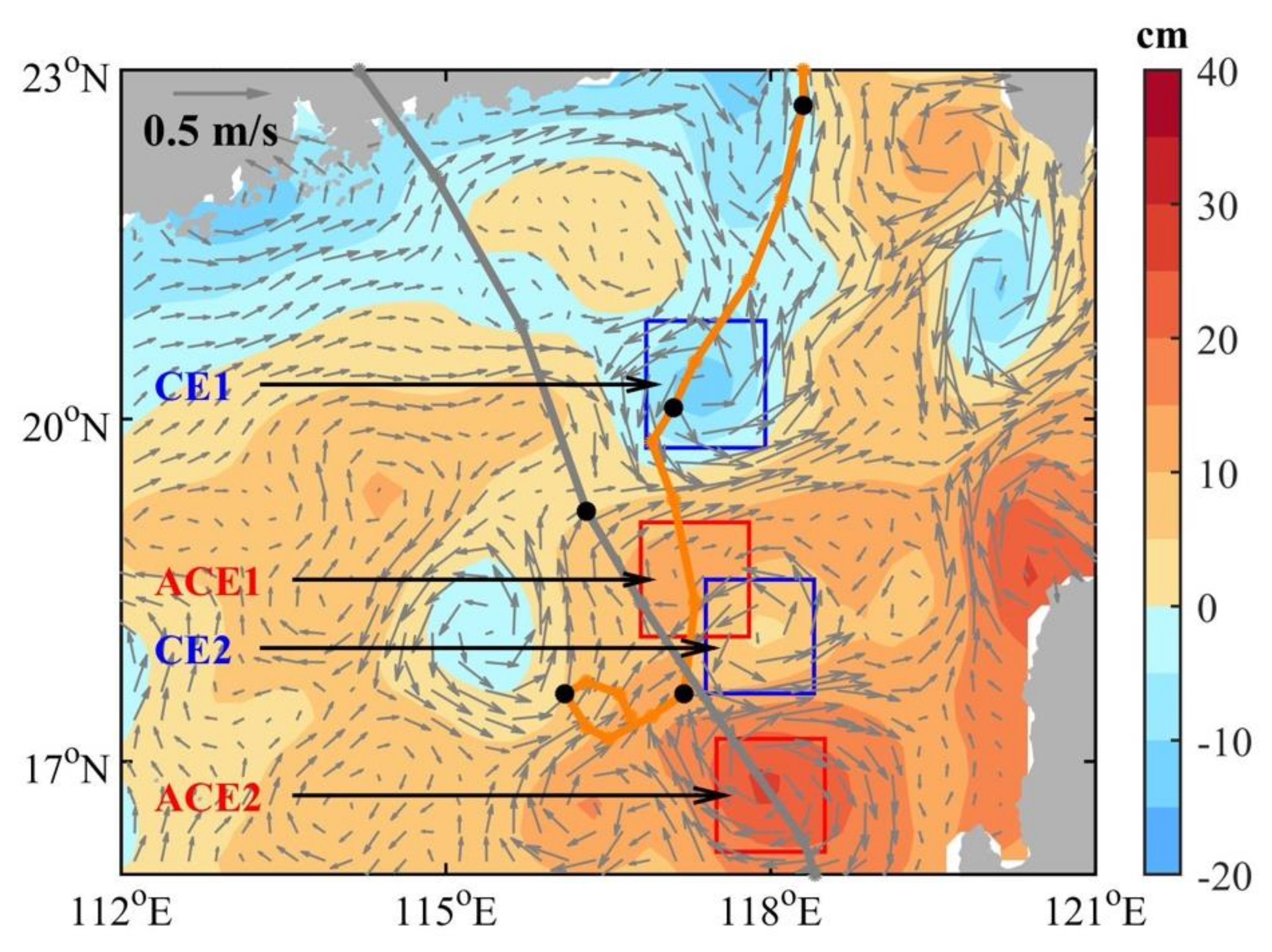
| Region of eddies | 116.8–117.9°E | 117.4–118.4°E | 116.8–117.8°E | 117.5–118.5°E | |
| 19.7–20.8°N | 17.6–18.6°N | 18.1–19.1°N | 16.2–17.2°N | ||
| Area of eddies (km2) | 13,981 | 11,718 | 11,684 | 11,811 | |
| Linfa (17–23 June) | Averaged position | 117.5°E | 117.8°E | 117.5°E | 118.0°E |
| 20.5°N | 18.2°N | 18.6°N | 16.8°N | ||
| Averaged radius (km) | 63.1 | 54.8 | 57.2 | 86.4 | |
| Maximum relative SLA (cm) | −7.8 | −5.7 | 7.4 | 10.7 | |
| Smallest distance to TY (km) | 4.75 | 45.34 | 11.48 | 108.90 | |
| Nangka (24 June–2 July) | Averaged position | 117.3°E | 117.8°E | 17.5°E | 118.0°E |
| 20.0°N | 18.2°N | 18.7°N | 16.8°N | ||
| Averaged radius (km) | 74.9 | 78.2 | 40.0 | 68.8 | |
| Maximum relative SLA (cm) | −7.4 | −5.6 | 0.6 | 11.6 | |
| Smallest distance to TY (km) | 112.36 | 65.22 | 65.50 | 4.08 | |
| CE1 | CE2 | ACE1 | ACE2 | ||
|---|---|---|---|---|---|
| Linfa | Period when typhoon passed over the eddy | 18 on 19 June–00 on 20 June | 00–06 on 19 June | 06–12 on 19 June | 06 on 17 June–00 on 19 June |
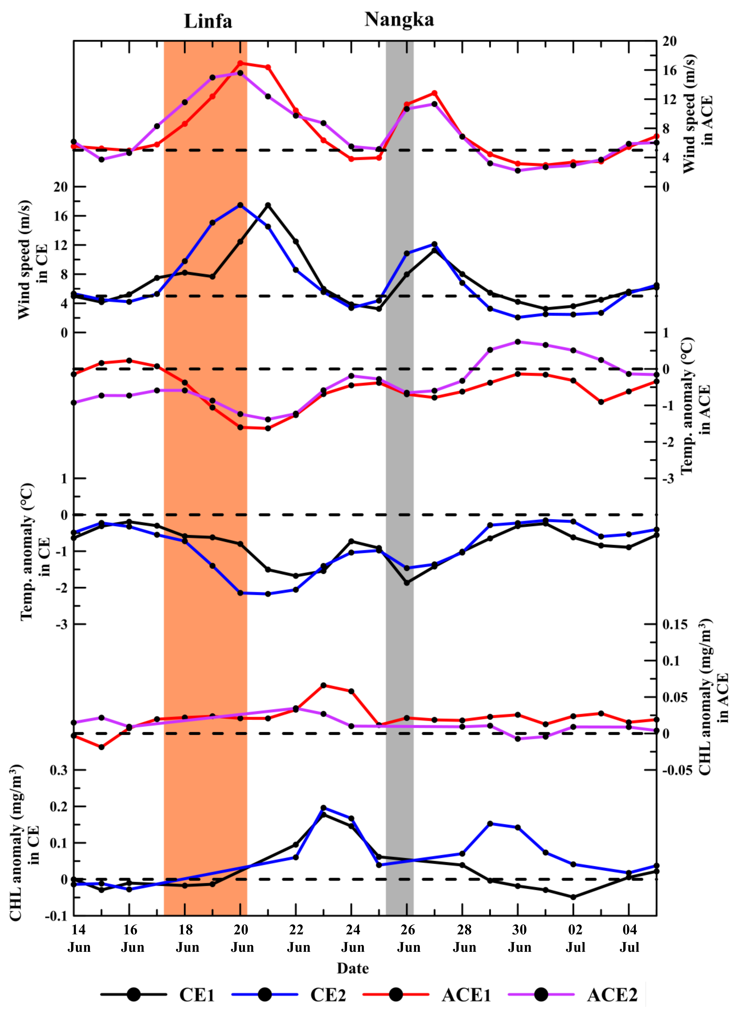
| Maximum ΔT (°C) | −1.68 | −2.17 | −1.63 | −1.38 | |
| Time for maximum ΔT | 22 June | 21 June | 21 June | 21 June | |
| Maximum ΔCHL | 0.17 | 0.20 | 0.07 | 0.03 | |
| Time for maximum ΔCHL | 23 June | 23 June | 23 June | 22 June | |
| Nangka | Period when typhoon passed over the eddy | 00–06 on 26 June | 18 on 25 June–00 on 26 June | 12–18 on 25 June | 06–12 on 25 June |
| Maximum ΔT (°C) | −1.86 | −1.46 | −0.78 | −0.65 | |
| Time for maximum ΔT | 26 June | 26 June | 27 June | 26 June | |
| Maximum ΔCHL | 0.04 | 0.15 | 0.03 | 0.01 | |
| Time for maximum ΔCHL | 28 June | 29 June | 30 June | 29 June | |
© 2020 by the authors. Licensee MDPI, Basel, Switzerland. This article is an open access article distributed under the terms and conditions of the Creative Commons Attribution (CC BY) license (http://creativecommons.org/licenses/by/4.0/).
Share and Cite
Jin, W.; Liang, C.; Hu, J.; Meng, Q.; Lü, H.; Wang, Y.; Lin, F.; Chen, X.; Liu, X. Modulation Effect of Mesoscale Eddies on Sequential Typhoon-Induced Oceanic Responses in the South China Sea. Remote Sens. 2020, 12, 3059. https://doi.org/10.3390/rs12183059
Jin W, Liang C, Hu J, Meng Q, Lü H, Wang Y, Lin F, Chen X, Liu X. Modulation Effect of Mesoscale Eddies on Sequential Typhoon-Induced Oceanic Responses in the South China Sea. Remote Sensing. 2020; 12(18):3059. https://doi.org/10.3390/rs12183059
Chicago/Turabian StyleJin, Weifang, Chujin Liang, Junyang Hu, Qicheng Meng, Haibin Lü, Yuntao Wang, Feilong Lin, Xiaoyan Chen, and Xiaohui Liu. 2020. "Modulation Effect of Mesoscale Eddies on Sequential Typhoon-Induced Oceanic Responses in the South China Sea" Remote Sensing 12, no. 18: 3059. https://doi.org/10.3390/rs12183059