Review

Deep Learning for Land Use and Land Cover Classification Based on Hyperspectral and Multispectral Earth Observation Data: A Review

Department of Electronics, Information and Bioengineering, Polytechnic of Milan University, Piazza Leonardo da Vinci 32, 20133 Milan, Italy
*
Author to whom correspondence should be addressed.
Remote Sens. 2020, 12(15), 2495; https://doi.org/10.3390/rs12152495
Submission received: 15 June 2020 / Revised: 28 July 2020 / Accepted: 29 July 2020 / Published: 3 August 2020

Abstract

:
Lately, with deep learning outpacing the other machine learning techniques in classifying images, we have witnessed a growing interest of the remote sensing community in employing these techniques for the land use and land cover classification based on multispectral and hyperspectral images; the number of related publications almost doubling each year since 2015 is an attest to that. The advances in remote sensing technologies, hence the fast-growing volume of timely data available at the global scale, offer new opportunities for a variety of applications. Deep learning being significantly successful in dealing with Big Data, seems to be a great candidate for exploiting the potentials of such complex massive data. However, there are some challenges related to the ground-truth, resolution, and the nature of data that strongly impact the performance of classification. In this paper, we review the use of deep learning in land use and land cover classification based on multispectral and hyperspectral images and we introduce the available data sources and datasets used by literature studies; we provide the readers with a framework to interpret the-state-of-the-art of deep learning in this context and offer a platform to approach methodologies, data, and challenges of the field.

Graphical Abstract

1. Motivation

The advances in remote sensing technologies and the resulting significant improvements in the spatial, spectral and temporal resolution of remotely sensed data, together with the extraordinary developments in Information and Communication Technologies (ICT) in terms of data storage, transmission, integration, and management capacities, are dramatically changing the way we observe the Earth. Such developments have increased the availability of data and led to a huge unprecedented source of information that allows us to have a more comprehensive picture of the state of our planet. Such a unique and global big set of data offers entirely new opportunities for a variety of applications that come with new challenges for scientists [1].
The primary application of remote sensing data is to observe the Earth and one of the major concerns in Earth observation is the monitoring of the land cover changes. Detrimental changes in land use and land cover are the leading contributors to terrestrial biodiversity losses [2], harms to ecosystem [3], and dramatic climate changes [4]. The proximate sources of change in land covers are human activities that make use of, and hence change or maintain, the attributes of land cover [5]. Monitoring the changes in land cover is highly valuable in designing and managing better regulations to prevent or compensate the damages derived from such activities. Monitoring the gradual—but alerting—changes in the land cover helps in predicting and avoiding natural disasters and hazardous events [6], but such monitoring is very expensive and labour-intensive, and it is mostly limited to the first-world countries. The availability of high-resolution remote sensing data in a continuous temporal basis can be significantly effective to automatically extract on-Earth objects and land covers, map them and monitor their changes.
Nonetheless, exploiting the great potentials of remote sensing data holds several critical challenges. The massive volume of raw remote sensing data comes with the so-called four challenges of Big Data referred to as “four Vs”: Volume, Variety, Velocity, and Veracity [7]. To mine and extract meaningful information from such data in an efficient way and to manage its volume, special tools and methods are required. In the last decade, Deep Learning algorithms have shown promising performance in analysing big sets of data, by performing complex abstractions over data through a hierarchical learning process. However, despite the massive success of deep learning in analysing conventional data types (e.g., grey-scale and coloured image, audio, video, and text), remote sensing data is yet a new challenge due to its unique characteristics.
According to [8], the unique characteristics of remote sensing data come from the fact that such data are geodetic measurements with quality controls that are completely dependent on the sensors adequacy, they are geo-located, time variable and usually multi-modal, i.e., captured jointly by different sensors with different contents. These characteristics in nature raise new challenges on how to deal with the data that comes with a variety of impacting variables and may require prior knowledge about how it has been acquired. In addition, despite the fast-growing data volume on a global scale that contains plenty of metadata, it is lacking adequate annotations for direct use of supervised machine learning-based approaches. Therefore, to effectively employ machine learning—and indeed deep learning—techniques on such data, additional efforts are needed. Moreover, in many cases remote sensing is to retrieve geo-physical and geo-chemical quantities rather than land cover classification and object detection, for which [8] indicate that expert-free use of deep learning techniques is still getting questioned. Further challenges include limited resolution, high dimensionality, redundancy within data, atmospheric and acquisition noise, calibration of spectral bands, and many other source-specific issues.
Answering to how deep learning would be advantageous and effective to tackle these challenges requires a deeper look into the current state-of-the-art to understand how studies have customised and adapted these techniques to make them fit into the remote sensing context. In this work, we explore the state-of-the-art of deep learning methodologies with the aim of finding full or partial answers to these challenges. Since the use of deep learning in this field is recent, a review that gives a comprehensive picture of where and how deep learning techniques are responding to these challenges is missing. In this work, not getting into single mathematical details of a single technique, we report the advances of deep learning in the field of land cover classification and discuss how the most used techniques are evolved, transformed, and fused to address specific challenges. Before that, we also provide an overview of research trends, critical terms, data characteristics, and available datasets.
The remainder of this paper is organised as follows: first, we give a short historical overview of land use and land cover classifications of remote sensing data and explain the current trends in this field. Then, we give a short introduction on Multispectral and Hyperspectral remote sensing data, followed by common datasets used for evidence-based research. Afterwards, we discuss the possible machine learning pipelines for land use and land cover classification and their pros and cons explaining how deep learning can be integrated into such pipelines. Furthermore, we go into more details on the different stages of the machine learning pipeline and on its common challenges explaining the use of deep learning to tackle also sub-tasks of the classical machine learning process. As a conclusion, we highlight the gaps and new challenges we found during this review opening the doors for further research lines in the field.

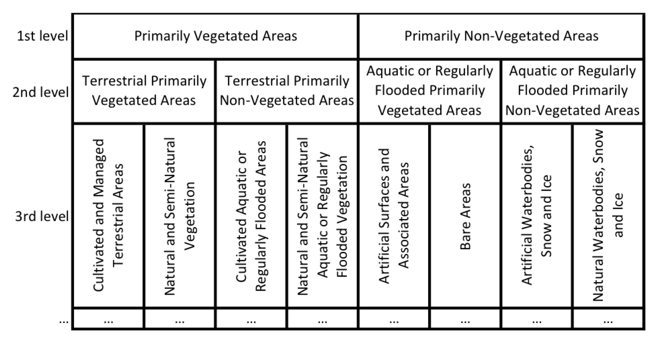
2. Land Use and Land Cover Classification

Land mappings of Earth are traditionally categorised into land use classification and land cover classification. Although in many studies these two concepts are interchangeable, or, as stated in [9], are confused by each other, the proper definition of each makes them different. According to the Food and Agriculture Organisation (FAO) [10] of the United Nations, “Land cover is the observed (bio)physical cover on the Earth’s surface”, while “Land use is characterised by the arrangements, activities and inputs by people to produce, change or maintain a certain land cover type”. According to the definition, land use and land cover are tightly related, and their joint classification is almost inevitable. Therefore, in recent studies “land use and land cover” (LULC) classification as a whole is considered as a more general concept also covering this relationship.
There are different taxonomies for LULC, based on the targeted applications; one of the most famous definitions belongs to FAO and offers a hierarchical land cover classification system (LCCS), which provides the ability to accommodate different levels of information, starting with structured broad-level classes, which allow further systematic subdivision into more detailed sub-classes [11] (Figure 1). This definition assures a high level of mappability that also covers the user-defined land use descriptors.
In general, studies approaching LULC classification consider a very small number of land cover or land use categories. Depending on the target application, these categories may be at the higher level of the hierarchy, distinguishing obvious land covers, or focussing on specific land cover sub-class categories. The classification of wetlands [12,13], urban land-use [14,15], agriculture [16], forest [17], and other vegetation mappings are some examples of the application-focused LULC classification approaches that are available in the literature.
The earliest use of remotely sensed data for the LULC classification goes back to mid-1940s when Francis J Marschner began to map the entire United States by associating the land uses to the Earth surface using aerial photography [18]. Years later, just after the launch of the Earth Resources Technologies research satellite equipped with a multispectral scanner (MSS) on July 1972 and the start of the Landsat program, the studies using the remotely sensed imagery data to classify the LULC stepped to a new level [19,20]. In fact, with the birth of the Landsat program and the (private) release of data, new challenges of multi-modal data fusion, land change detection on a temporal basis, and ecological applications of the satellite data, were introduced to the field of LULC. Some of the early works on these topics are discussed by [21,22,23,24].
The studies over LULC classification and its further challenges are constantly and rapidly evolving as the result of the fast improvements in the processing and storage capacity of computers and the evolution in Artificial Intelligence (AI). Moreover, any advance in the remote sensing technologies, and in the quality of data, comes with new opportunities for researchers to extract new information from the remote sensing data [25]. The growing trend of publications about the LULC classification of remote sensing data is pictured in Figure 2. The trend has been captured searching for a set of key terms in the title, abstract and keywords of all documents available in Scopus, grouped and filtered by five-year intervals.
The trends in Figure 2 contain four different search results: the first one (Blue) is the count of publications on LULC classification/segmentation using all types of remote sensing data. The second one (Orange) restricts publications on LULC classification/segmentation to hyperspectral data: this emphasises an increasing number of studies working on such data in the last two decades. The third one (Green) shows the use of “deep learning” techniques in LULC classification with all types of remote sensing data, emerged in the last years (interested readers can find a review on such publications in [26]). The last one (Red) restricts the latter type considering only the use of multispectral and hyperspectral remote sensing data, which are increasingly getting attention due to their recent availability.
Hyperspectral imaging, being tied to the advances in digital electronics and computing capabilities, was embraced later by the Earth Observation community due to its complexity in nature and the computational limitations of the time. However, the great potentials of such data, its availability, and the fast developments in computational technologies are increasingly attracting scientists interested in LULC classification. Moreover, the extraordinary achievements of deep learning since the ImageNet Large Scale Visual Recognition Challenge (ILSVRC) [27], encouraged remote sensing scientists to employ these techniques on remote sensing data as well, starting from 2015. Reference [28] devote their study to the challenges of hyperspectral imaging technologies and review the state-of-the-art of deep learning methodologies used for hyperspectral image classifications. Reference [29] also presents an overview of deep learning methods for hyperspectral image classification and compare the effectiveness of these methods on common well-known datasets.
In this review paper, we explore this recent growing research trend in using deep learning techniques for LULC classification of hyperspectral and multispectral images, as both data types have significant common attributes that can be studied together. The main aim is to draw up a lively document that gives a framework about how to read the state-of-the-art of deep learning in the field of LULC classification of remote sensing data, with an emphasis on hyperspectral and multispectral images. The focus of this document is to provide a platform for the readers to extract proper methods and datasets to address the existing challenges of the field.
Considering Figure 2, this paper reviews the papers highlighted in red (LULC classification of hyperspectral and multispectral remote sensing images using deep learning techniques) obtained with the search query: TITLE-ABS-KEY(“deep learning” OR “convolutional neural network” AND “land cover” OR “landcover” OR “land use” OR “landuse” OR “lulc” AND “multispectral” OR “multi spectral” OR “hyperspectral” OR “hyper spectral”). We considered the documents that were cited by these selected articles and other works that these selected articles were cited by. Going through these sources helped us sketch the general schema of the state-of-the-art you find in the following, focusing on the position of deep learning in the whole picture. As a side note, we stress here a clarification for the reader about the use of the term “land cover classification” in literature as in several works it actually refers to “land cover segmentation”. In other words, the classification term refers to the pixel level, hence the final targeted result is a segmented map. In some works, the aim of classification is instead a patch-based classification, where a fixed size patch of an image is assigned to a specific class. In this review paper, for clarity, these approaches are referred to as “pixel-level classification” and “patch-level classification”, respectively. For the sake of simplicity, we adopt the term “land cover classification” for pixel-level classification, when not explicitly specified.
From a formal point of view, the LULC classification process is defined as f : X Y , with input space X N W × H × K where W , H , K are respectively the width, height and number of spectral bands for each input image, which the output space for pixel-level land cover classification and patch-level land cover classification is represented as Y C W × H and Y C respectively, where C = { Ω 0 , Ω 1 , Ω k } is the set of possible land use and land cover categories.

3. Multispectral and Hyperspectral Remote Sensing Data

Remotely sensed images are usually captured by optical, thermal, or Synthetic Aperture Radar (SAR) imaging systems. The optical sensor is sensitive to a spectrum range from visible to mid-infrared of the radiations emitted from the Earth’s surface, and it produces Panchromatic, Multispectral or Hyperspectral images. Thermal imaging sensors, capturing the thermal radiations from the Earth surface, are instead sensitive to the range of mid to long-wave infrared wavelengths. Unlike thermal and optical sensors that operate passively, the SAR sensor is an active microwave instrument that illuminates the ground scattering microwave radiations and captures the reflected waves from the Earth’s surface.
The panchromatic sensor is a monospectral channel detector that captures the radiations within a wide range of wavelength in one channel, while multispectral and hyperspectral sensors collect the data in multiple channels. Therefore, unlike the panchromatic products that are mono-layer 2D images, hyperspectral and multispectral images share a similar 3D structure with layers of images, each representing the radiations within a spectral band. Despite the similarity in the 3D structure, the main difference between multispectral and hyperspectral images is in the number of spectral bands. Commonly, images with more than 2 and up to 13 spectral bands are called multispectral, while the images with more spectral bands are called hyperspectral. Nevertheless, the main difference is that the hyperspectral acquisition of spectrum for each image pixel is contiguous, while for multispectral it is discrete (Figure 3—Left).
Having hundreds of narrow and contiguous spectral bands, hyperspectral images (HSI) come with specific challenges intrinsic to their nature that do not exist with multispectral (MSI) and panchromatic images. These challenges include: (1) High-dimensionality of HSI, (2) different types of noise for each band, (3) uncertainty of observed source, and (4) non-linear relations between the captured spectral information [31]. The latter is explained to result from the scatterings of surrounding objects during the acquisition process, the different atmospheric and geometric distortions, and the intra-class variability of similar objects.
Despite the mentioned differences in the nature of MSI and HSI, both share a similar 3D cubic-shape structure (Figure 3—Right) and are mostly used for similar purposes. Indeed, the idea behind LULC classification/segmentation relies on the morphological characteristics and material differences of on-ground regions and items, which are respectively retrievable from spatial and spectral information available in both MSI and HSI. Therefore, unlike [32] that review methodologies designed for spectral-spatial information fusion for only hyperspectral image classifications, in this review we consider both data types as used in the literature for land cover classifications using deep learning techniques focusing on the spectral and/or spatial characteristics of land cover correlated pixels.

Data Sources and Datasets

There are many satellite and airborne imagery providers that release timely and high-resolution remote sensing data to the public without any cost. USGS [33,34], NEO [35], Copernicus open access hub [36], NASA Earth data [37], NOAA [38,39] and IPMUS Terra [40] are among the most popular open access remote sensing data providers. In the literature, satellite images used for deep learning purposes are mostly obtained from Landsat-7, Landsat-8, Sentinel-1, Sentinel-2, WorldView-2, WorldView-3, QuickBird, EO-1, PROBA-1, and SPOT-6 satellites. Table 1 presents a short overview of the status of these satellites and their image products. Except for Sentinel-1, EO-1, and PROBA-1 that produce both SAR and hyperspectral images, the products of the other satellites listed in the table are multispectral images. As explained before, panchromatic band images (black and white) are captured by a single channel detector that is sensitive to a broad wavelength range, coinciding with the visible range, which collects a higher amount of solar radiation. Therefore, the spatial resolution of panchromatic images is usually higher than the MSI. Landsat, WorldView, SPOT-6 and QuickBird capture panchromatic images together with MSI. Among the MSI providers, Sentinel-2, with the highest number of spectral bands (13 bands) and highest orbital altitude among these satellites, is the only mission that can provide data with global coverage data in five days.
Among the satellites in Table 1, the highest resolution images are obtained by WorldView-3 and WorldView-2, followed by QuickBird and SPOT-6 satellites. All these satellites are commercial, therefore their images are expensive and available in open access with limited land coverage. In the literature, very high resolution multispectral and hyperspectral images used for object detection, building and road extraction, or crop analysis, are mainly airborne images captured by digital sensors, such as AVIRIS and ROSIS. The spatial resolution of images of such sensors may vary depending on the altitude of the aircraft.
To exploit airborne or spaceborne images, supervised techniques are usually utilised. Such techniques infer the logic for classification based on labelled training data. However, explicitly labelling the data and collecting ground-truth for such supervised approaches is a complex and time-consuming task. Few available databases come with ground-truth. The most used datasets in the literature, already labelled, for land cover classification using deep learning techniques are graphically shown in Figure 4, and detailed in Table 2. In some of these datasets, the images are also properly cropped, corrected and archived in a way that is easy for the machine to retrieve and process.
Indian pines [45] and University of Pavia [45] datasets are used in many papers. Both datasets contain pixel-level ground-truth, and the images are captured by airborne hyperspectral imaging sensors. Indian pines dataset is taken by the AVIRIS sensor, which captures 224 band hyperspectral images. The dataset targets LULC in the agriculture field. Commonly, the studies using the Indian pines dataset remove the water absorption bands and consider only 200 spectral bands for the images. Salinas [45] data types are very similar to Indian pines, captured by the same sensor, targeting different agriculture classes. The University of Pavia dataset is captured by the ROSIS airborne sensor: resulting images have 103 spectral bands. The dataset is very similar to Pavia city centre [45], just a couple of classes are different (Pavia city centre has water and tile classes, while Pavia University has gravel and painted sheet classes). University of Pavia dataset is more popular as it has more samples for training.
GRSS 2013 [46], Kennedy space centre (KSC) [45], Botswana [45] and Cuprite [45] single images are other airborne pixel-level labelled imagery datasets used for land cover classification. DeepGlobe [47] (the land cover dataset) is a new pixel-level labelled dataset introduced in 2018 for the CVPR2018 challenge. It provides a huge number of pixel training samples, with high pixel resolution, but it contains only the RGB channels. The images of DeepGlobe dataset are the result of different commercial satellite image fusion, but there is no accurate indication on which sensors are used and how the images are fused.
Training samples with pixel-level labels are used for image segmentation. Therefore, the aforementioned datasets are in general adopted to classify the map pixels and to generate a segmented map. On the other hand, there exist also some datasets for which image patches are labelled with single or multiple tags. Sat-4 [48], Sat-6 [48], UCMerced [49], and Brazilian Coffee scenes [50] datasets are among the most popular patch-level labelled datasets. In addition to the commonly used datasets, some tools provide the users with access to annotated/semi-annotated databases, which are usually collected by combining information from different resources that target particular uses, for example, crops [51,52], forests [53], or wetlands [54] monitoring.
In general, almost all available labelled MSI and HSI datasets come with common limitations to apply supervised machine learning techniques. Effective use of supervised machine learning techniques requires a large number of training samples that should also cover different in-class variations. Since labelling of such data is quite slow, costly and labour intensive, these datasets are usually limited in the number of samples, lack variety and are too case-specific. Such limitations are mainly referred to as the limited ground-truth challenge, which will be discussed later in this paper.

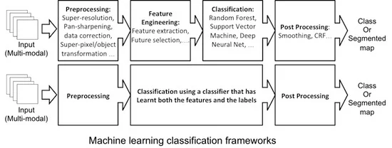
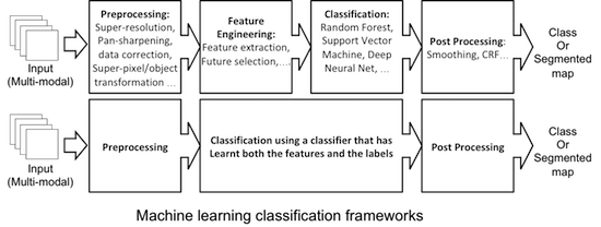
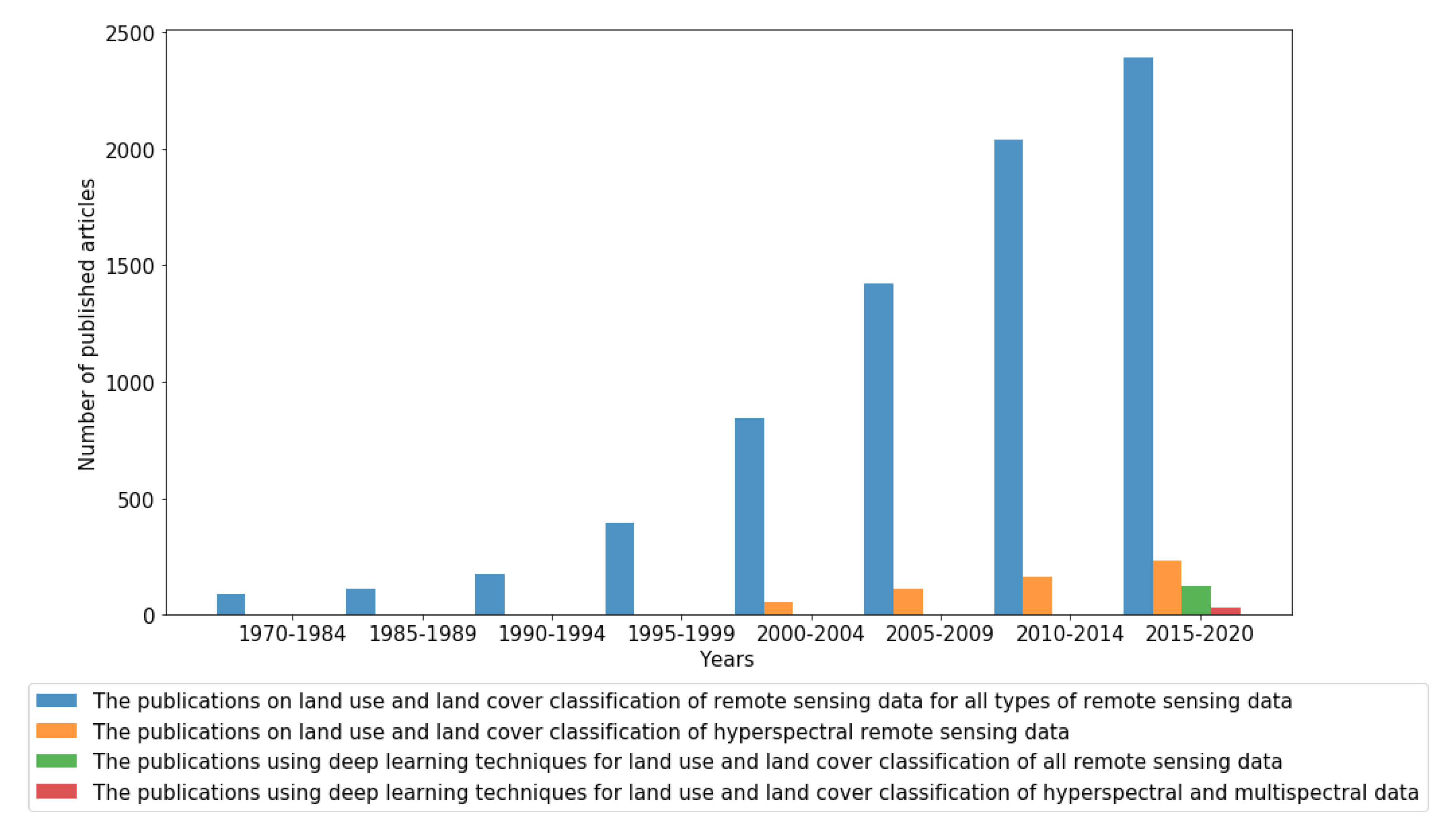
4. Machine Learning for LULC

Conventional supervised LULC machine learning pipelines usually include four major steps: (1) pre-processing, (2) feature engineering, (3) classifier training and (4) post-processing (Figure 5—top). Each of these stages may be composed of a set of sub-tasks. A good break down of the whole process into its sub-tasks, with an explicit statement of their assumptions, helps to define standalone sub-problems that can be studied independently and have solutions or models that can be incorporated into an LULC pipeline to accomplish the targeted classification/segmentation. Over the last years, with the growing popularity of deep learning as a very powerful tool in solving different types of AI problems, we are witnessing a surge in demand of research to employ deep learning techniques in tackling these sub-problems.
Specific sub-tasks are defined to tackle the needs of the above four stages of a machine learning pipeline; usually, the pre-processing stage includes the sub-tasks within which the input data get prepared for the following stages (i.e., feature engineering and classifier training). The preparation may require to correct, de-noise, synchronise, or fuse the data to come up with an enhanced version of the original input and to improve the whole process performance. The feature engineering phase is usually referred to as a set of feature extraction, selection, and transformation tasks, to remove redundant information from the processed input data, reducing its dimensionality, and defining a set of good representations (features) for the input, based upon which the machine can build a model to predict the target classes. The heart of the workflow is the classifier training, where the machine builds a mathematical model based on the training samples and understands the correlation between the training data features/representation and its pre-defined classes. The model, after being trained, tested and validated, is used to predict and classify the new data. Finally, the post-processing phase, in pixel-level classification, is usually a set of methods applied to enhance the final segmented image, by emphasising the morphological properties of classes or objects.
With the increased computational capacity in the new generation of processors, over the last decade, the end-to-end deep learning approach received lots of attention from the scientists. The end-to-end learning pipeline—taking the source data as the input-end and the classified map as the output-end—is a modern form of re-designing the process workflow, that is taking advantage of deep learning techniques in solving complex problems. Within the end-to-end deep learning structure, the feature engineering is replaced by feature learning as a part of the classifier training phase (Figure 5-bottom). In this case, instead of defining the inner steps of the feature engineering phase, the end-to-end architecture generalises the model generation involving feature learning as part of it. Such improved capacity of deep learning has promoted its application on many research works where well-known, off-the-shelf, end-to-end models are directly applied to new data, such as remote sensing. However, there are some open-problems, complexities, and efficiency issues in the end-to-end use of deep learning in LULC classification, that encourages us to adopt a new approach for investigation of the state-of-the-art in deep learning for LULC classification.
In the next sections, we have collected the state-of-the-art in using deep learning techniques for the LULC classification of HSI and MSI, considering their use in an end-to-end approach or in one of the phases of the traditional approach, including the training of land-cover classifier, the ground-truth generation, data fusion, data pre-processing and output post-processing stages. In particular:
  • In Section 4.1 and Section 4.2 we explain the feature learning property of an end-to-end approach and its limitations that lead us to consider the conventional machine learning model including feature engineering steps. Then we explain the concept of feature engineering, its components, and the common methodologies, as well as deep learning techniques employed in literature to accomplish them. We also discuss the importance of defining the feature space and its direct impact on shaping the process pipeline.
  • In Section 4.3 we explore the choices of MSI and HSI classifiers for the LULC classifications and discuss the effectiveness of deep learning techniques for this task. We also explain different types of deep learning approaches in classifying MSI and HSI used in the state-of-the-art.
  • Focusing on the well-know challenge of limited ground-truth, in Section 4.4 we explain how it impacts the performance of deep learning models for HSI and MSI. Then, we report the research works facing this challenge.
  • In Section 4.5 we discuss the challenge of data fusion as faced by many state-of-the-art studies. We explain the main concerns in data fusion and how deep learning is facilitating their accomplishments.
  • Finally, in Section 4.6 we discuss other potential pre-processing and post-processing techniques in literature that can improve the LULC classification performance.

4.1. End-To-End Deep Learning

As explained before, the increased computational capacity has popularised the end-to-end deep learning approaches, wherein instead of engineering the features, the features are automatically learnt by the classifier (Figure 5—bottom). In other words, in such approaches, the gradient-based learning is applied to the system as a whole. The end-to-end use of deep learning models has been very popular within the remote sensing community over the last years. The majority of the works compare the performance of such architecture with classical techniques, like for example, Support Vector Machine (SVM) and Random Forest (RF) classifiers [16]. However, the use of deep learning as an end-to-end approach comes with some complexities and inefficiencies in the processing time.
One insight is based on the Wolpert’s “No Free Lunch” (NFL) theorem [55] (the theorem was later developed in collaboration with Macready [56]), which states that “any two optimisation algorithms are equivalent when their performance is averaged across all possible problems” [56]. This implies that there is no single supervised learning algorithm, out of a set of uniformly distributed possible functions, that performs the best for all kinds of problems. This theorem refutes the idea of a generalised single machine learning algorithm for all types of problems and data, and underlines the need to check all assumptions and if they are satisfied in our particular problem. In practice, such deep learning models have shown a great capacity to generalise well, which is theoretically unclear and it is still getting questioned [57,58,59,60].
A second open issue is that, to automatically generate a hierarchy of abstractions, the deep learning models require a massive amount of training samples annotated with the targeted classes. In the case of end-to-end approaches for land cover classification of HSI and MSI, the massive amount of training samples should well cover the output-end’s class distributions. However, as stated in the previous section, due to difficulties in the collection of LULC ground-truth, it is subjected to the issue of the limited number of training samples.
Even if we could find an effective solution to increase the size of training datasets, for example, via unsupervised or semi-supervised learning, the issue of processing efficiency remains. As discussed in Section 1, the complexities in the nature of remote sensing data, such as multi-modality, resolution, high-dimensionality, redundancy and noise in data make it even more complex and challenging to model an end-to-end workflow for the LULC classification of MSI and HSI. The more complex the model architecture becomes, the more difficult the learning problem gets. In other words, increasing the complexity of deep learning architectures leads to more difficult optimisation problems and dramatically decreases the computational efficiency.
Therefore, despite the substantial attempts in applying end-to-end deep learning in LULC classification problems, the challenges of such structure open up the floor for alternative approaches and make the former four-stage machine learning pipeline structure a debatable candidate. Indeed, defining the process according to a conventional workflow format makes it easier to shape, customise, and adapt the system to meet the targeted needs and, at the same time, it reduces the model optimisation complexity and computational time of the learning process. Breaking down the assumptions, needs, and targets into a set of sub-tasks, the empirical process of choosing an effective algorithm for each sub-task becomes easier and more diagnosable. Indeed, we can employ deep learning techniques more effectively and transparently to accomplish single sub-tasks of a classical machine learning pipeline with smaller problems to solve. All the solutions and trained models for each sub-task can be then employed in parallel streams or in sequential order at different steps of the conventional workflow. For instance, the authors in [61] propose a model seeing the feature selection problem as a feature reconstruction problem using a deep belief network and compare its efficiency in time with a deep CNN end-to-end model. Or to deal with the ground-truth scarcity problem, the work in [62] proposes the use of deep learning in a semi-supervised generative framework that can deal with feature extraction from a small number of samples.

4.2. Feature Engineering

Feature engineering is one of the steps in the conventional LULC machine learning pipeline, before the classifier training, that deals with the definition of features (or representations) that better fit the classifier requirements. “Features are the observations or characteristics on which a model is built, and the process of deriving a new abstract feature based on the given data is broadly referred to as feature engineering” [63]. Feature engineering aims to reduce the size of input data and to transform it into a set of representations that carry only its relevant meaningful information. Building a model on large raw datasets, with a large number of attributes per data possibly with some redundancies, is computationally expensive and inefficient. Therefore, transforming the raw data into a manageable set of meaningful representations is very critical to build a model effectively. Commonly, different forms of feature engineering are referred to as feature selection, feature transformation, and feature extraction.
Feature selection and feature transformation are usually referred to as dimensionality reduction techniques. In particular, the aim of feature selection is to remove the irrelevant or redundant information of the data, possibly without altering the rest of the information in data. On the other hand, feature transformation maps the input into an alternative space, to make the process easier. Selecting and transforming features may be a manual task dealt with based on expert prior knowledge or can be automated employing machine learning techniques.
Feature extraction is mainly used to reduce the number of data features, by creating a new set of features out of the existing ones. In classical machine learning approaches, the feature extraction task, also called hand-crafting features, calculates the set of new representations using predefined algorithms. Thanks to deep learning, feature extraction can be also conducted automatically, without dealing with the complexity of designing and formulating proper algorithms.
The HSI and MSI are cubic types of data [64] that contain two spatial dimensions (the width and height of channels) and one spectral dimension (number of channels). The spatial domain contains the morphological information and the spectral one is to distinguish material that corresponds to a pixel on the ground. Indexing the data in the time order adds another dimension to the data space, and it comes with time-series challenges. Transferring such a complex 3 or 4-dimensional space into a feature space with relevant information is very critical. The dimension of the feature space is defined based on the interrelation among the spatial, spectral, and temporal aspects of data. In some works, all these aspects are considered independent, while others are considered partially or fully dependent. The prior assumption on the dependency or independence of such features plays a crucial role in the design of the machine learning pipeline, the choice of the classifier, and the feature engineering steps.
Feature engineering is very challenging for HSI data. There are three problems to be considered: (1) the high number of spectral bands leads to the problem of high-dimensionality, the so-called curse of dimensionality [65]: with limited training samples it implies that much of the hyperspectral data space is empty, i.e., it does not have any observation upon which it can build a model; (2) the correlation between the spectral bands is not necessarily linear; and (3) the similarity between some spectral bands denotes the high spectral interband redundancy in a way that reducing some spectral bands does not cause significant loss of information. Therefore, to extract proper representations from the spectral domain of HSI data, feature transformation and feature selection should be considered together with the feature extraction. In this way, it is possible to reduce dimension and to remove redundancy, which helps translate data into manageable and learnable representations. The work in [66] deeply discusses the differences in techniques and tools to implement the feature extraction of HSI.
Feature engineering of data is of high value when the amount of training samples does not satisfy the end-to-end learning requirement, or when the learning of representations through the end-to-end approach is not computationally efficient. Nevertheless, the feature engineering stage can still benefit from deep learning and other machine learning techniques to find good representations for the data. In the next subsections, we explain feature selection, transformation and extraction for HSI and MSI data, and we discuss the common machine learning techniques, including deep learning techniques, used to tackle these tasks.

4.2.1. Feature Selection and Transformation

Feature selection and feature transformation of data are mostly referred to as dimensionality reduction techniques. Feature selection aims at removing redundancy by selecting the relevant attributes of the data, while feature transformation maps the data into another simpler space with possibly smaller dimension. Although, selecting and transforming the data into a set of relevant manageable representations that are compatible to the classifier requirements can significantly improve the performance of the machine, reduce the overfitting possibility, and cut down the training time, an excessive reduction of information can also go in the opposite way. Therefore, transformation and selection of features are quite challenging and sensitive.
The most common dimensionality reduction algorithm used for HSI data is the Principal Component Analysis (PCA) [67,68,69]. PCA projects the data into a new space within which the dimensions are linearly independent (orthogonal), and they are ranked in such a way that the principal axis is the one that the data is more spread in [70]. Therefore, PCA transforms the data into a simpler space for analysis, tackling feature transformation to reduce the feature dimension upon which the model is built.
Feature selection, also referred to as data cleaning or data filtering, removes redundancies in data and keeps the most relevant attributes to create a set of features for building a model. It reduces the chance of overfitting and the time of training, and eventually improves the accuracy of the classification. In almost all stochastic learning techniques, the importance of the features is calculated automatically through the classifier training phase. Feature importance ranking shows the importance of input data attributes, so it makes clear which attributes of the input data are potentially removable. Feature selection for complex HSI and MSI data, with a huge amount of attributes, is two-fold; With classical machine learning classifiers, such as SVM, the feature selection is crucial as defining the hyper-parameters for massive input types is too complex and impractical [71,72]. However, with the modern classifiers designed to avoid the overfitting problem, the necessity to reduce information from input data is questionable [73,74].
The use of deep learning in the feature engineering phase is mainly referred to as feature extraction. A feature engineering deep learning model learns how to optimally transform the input space into a smaller coded space that includes all its important information. Usually, the important information is referred to as the coded features that are enough to reconstruct the input with. In the following subsection, the feature extraction methodologies based on deep learning techniques are discussed.

4.2.2. Feature Extraction

Feature extraction defines a new set of representations, or abstractions, for data based on all existing attributes in it, to make the training process easier for the machine. A good set of representations contains all relevant information that fits the classification requirement. Such representations can be hand-crafted, using algorithms that calculate a new set of features. For instance, the well-known NDVI (Normalised Difference Vegetation Index) is a simple example of hand-crafting features, simply combining NIR (Near Infrared) and red bands of the image, and is very informative for detecting vegetation on land cover. Refs. [13,75] use NDVI masks and other indices to guide the Convolutional Neural Network (CNN)-based model (the technique is explained in Section 4.3) in detecting vegetation, water and other elements which are highlighted by these masks. Hand-crafting features can be also obtained by using image processing techniques, such as edge detection, smoothing, or segmentation.
Unsupervised, semi-supervised, and supervised machine learning techniques can also extract relevant features for the classifier. The best known unsupervised machine learning techniques to extract features automatically are the deep learning Autoencoder (AE) techniques (the technique is explained in Section 4.3). Over the last few years, AE algorithms have become very handy and popular to extract the optimised abstraction of HSI and MSI data for the classifier [76,77,78]. Although such unsupervised algorithms can find the data representations without any hint or label, ref. [79] underline the advantages of using supervised algorithms, pointing out that not only the global mutual information but also the in-class discriminative projections have to be explored in HSI data. Supervised algorithms using labelled samples can learn metrics that keep data points within a class together and separate them from the other classes [80]. Since the preparation of labelled data for supervised techniques is quite labour-intensive, conventional supervised algorithms can be extended to the semi-supervised variants [81]. The main supervised/semi-supervised dimension reduction algorithms applied on HSI data are based on different types of discriminant analysis, for example, Linear Discriminant Analysis (LDA), Stochastic Discriminant Analysis (SDA), and Local Fisher Discriminant Analysis (LFDA), ref. [82,83,84] and Local Discriminant Embedding (LDE) and Balanced Local Discriminant Embedding (BLDE) [80,85].

4.3. Classifier

Despite the growing popularity of deep neural networks, the classic supervised classifiers are still popular within the remote sensing community. RF and SVM are the most-common classic classifiers used in literature for the land cover classification of remote sensing data. Like the other non-parametric supervised classifiers, these algorithms do not make any assumption regarding the distribution of data and they have shown promising results in classifying remote sensing data overtaking the field’s earlier classifiers adopted such as Linear Regression (LG), Maximum Likelihood (MLC), K Nearest Neighbor (KNN) and Classification and Regression Tree (CART).
RF is an ensemble classifier made of a set of tree-structured predictors (CARTs) such that each tree depends on a random set of training observations that are sampled independently with replacement [86] and, at each splitting node of the trees, a subset of features is randomly selected to grow the tree [87]. RF is pretty popular for classifying remote sensing data due to its simplicity and its power in reaching robust models. It has been broadly used to classify the land cover [88,89,90], and many other applications as reported in [91]. However, like the majority of supervised classifiers, RF requires an adequately big set of reference data to learn the class distributions, which is often a critical problem.
SVM is another popular classifier for remote sensing data that works well with a relatively small amount of training samples. The algorithm aims at finding an optimal separating hyperplane that separates the observations into target classes so that the boundaries among the classes minimise the misclassification rates [92]. The regularisation parameter in SVM plays a critical role in its performance; with well-tuned regularisations, SVMs tend to be resistant to overfitting and do not have any inherent problem when the number of observations is less than the number of attributes [93,94]. Relying on such characteristics, SVM has been very popular for land cover classification of MSI and HSI [95,96,97].
However, when it comes to complex problems such as classification of HSI images, deep learning approaches with the capability to learn from hierarchies of features, outperform the other classifiers. Deep learning models are composed of multiple layers such that each layer computes a new data representation from the representation in the previous layers of artificial neurons creating a hierarchy of data abstractions [98]. CNNs are a group of deep learning techniques that are composed of convolution and pooling layers that are usually concluded by a fully connected neural network layer and a proper activation function, i.e., in models that directly reconstruct an output image prediction, such as U-Net and generative models (explained later on), the fully connected network and activation function is not needed. CNNs, being very successful in classifying complex contextual images, have been widely used to classify remote sensing data too.
CNNs are feedforward neural networks (artificial neural networks wherein no cycle is formed by the connections between its nodes/neurons) that are designed to process the data types composed of multiple arrays (e.g., images, which have layers of 2D-array of pixels) [98]. Each CNN, as shown in Figure 6, contains multiple stages of convolution and pooling, creating a hierarchy of dependant feature maps. The example in the figure shows convolutional neural networks with two layers of convolution and two layers of pooling, for (a) patch-level classification, (b) pixel-level classification and (c) an image reconstructive model. In (a) and (b) a fully connected network is fed with the flattened feature maps of the latest pooling layer. In (b) the central part is shown in red is the pixel to which the class is assigned. In (c), the model does not include any fully connected network and activation function, but the right half part of the model directly reconstructs an output image predication.
At each layer of convolution, the feature maps are computed as the weighted sum of the previous layer of feature patches, using a filter with a stack of fixed-size kernels, and then pass the result into non-linearity, using an activation function (e.g., ReLU). In such a way, they detect local correlations (fitted in the kernel size), while keeping invariance to the location within the input data array. The pooling layer is used to reduce the dimension of the resulted feature map by calculating the maximum or the average of neighbouring units to create invariance to scaling, small shifts, and distortions. Eventually, the stages of convolution and pooling layers are concluded by a fully connected neural network and an activation function, which are in charge of the classification task within the network.
The process of training a CNN model, using a set of training samples, finds optimised values for the model learnable parameters, by reducing the cost calculated via a loss function (e.g., Minimum Square Error, Cross Entropy, or Hinge loss). In CNNs, learnable parameters are the weights associated with both convolution layer filters and connections between the neurons in the fully connected neural network. Therefore, the aim of the optimiser (e.g., Stochastic Gradient Descent, RMSprop, or Adam) is not only to train the classifier, but it is also responsible to learn data features by optimizing convolution layers parameters.
The size and dimension of filters for each convolution layer are the so-called model hyper-parameters. Although choosing the kernel size for the filters is usually an inductive process, the dimension of filters can be directly driven from a prior knowledge over the input space (e.g., time-series, one channel image, multi-channel image, or time-series of multi-channel images) and over the expectations on the type of features to be extracted (e.g., spatial, spectral, spatial-spectral, or spatial-spectral-temporal features). The CNNs used in the literature for classifying remote sensing data can be categorised into three sub-types: CNN with one-dimensional filters (1D-CNN), CNN with two-dimensional filters (2D-CNN), and CNN with three-dimensional filters (3D-CNN), shown in Figure 7. The differences in the mentioned sub-types of CNN are at the convolution layers. These networks may be used jointly in parallel streams to extract different independent features.
One-dimensional CNNs, mostly used for time series modelling, have also been used to extract the spectral features of pixels in HSI data [99,100,101]. This technique is sometimes called spectral curve classification [101]. Stacking the spectral layers of an HSI corresponding to three seasons on top of each other, ref. [102] apply 1D-CNN to also distinguish the seasonal change feature in the spectral-temporal domain. Reference [103] propose a hybrid model of 1D-CNN and RNN that learns the spectral dependencies automatically. In particular, it is composed of layers of convolution and pooling (to extract locally-invariant features), followed by recurrent layers (to retrieve the spectrally-contextual information from the latter extracted features), and concluded by a fully connected neural network and an activation function. Reference [104] use 1D-CNN in a generative adversarial network (1D-GAN) to generate fake spectral data, and also as a discriminator to classify the spectral features.
Two-dimensional CNN is the common type of CNN, used to classify images where there is a correlation between the morphological details and the target classes. In remote sensing, 2D-CNN is typically adopted to extract the spatial features of the HSI and MSI, considering the continuity of land covers in the spatial domain [105].Well-known CNN pre-defined models, developed for image understanding, are sometimes used in literature to classify land covers, including LeNet5 [106], AlexNet [107], VGGNet [108], CaffeNet [109], GoogLeNet [110] and ResNet [111] models. In [8,112], authors have compared the mentioned models in the context of land cover classification of HSI. In general, as the relation among spectral bands of HSI is not linear, 2D-CNNs are usually used jointly with 1D-CNNs to cover the spectral-spatial domain of features of HSI data [99]. In such cases the models extract spatial and spectral features separately in parallel, then their extracted features are normally put together and fed to a fully connected classifier followed by an activation function. However, since combining the extracted features in such a structure is an additional empirical process, fine-tuning the model gets even more complex [113]. Three-dimensional CNN is an alternative approach that can reduce this complexity by simply leaving the features as tensors in a 3D space, considering also potential correlations between the spatial and spectral aspects of data.
Three-dimensional CNN is mostly used for multi-frame image classification in which the temporal dimension is added to the domain (spatio-temporal classification). In the case of remote sensing, 3D CNNs are used to extract spectral-spatial [114,115] and spatial-temporal [113] features. In such classifications, the features are assumed as tensors in 3D domains, and each layer of convolution-pooling affects the size of feature volume in depth, width and length. Authors in [73], focusing on the full utilisation of spectral and spatial information in input HSI data, propose an end-to-end model that contains four sequential residual blocks with 3D CNNs to extract the spectral and spatial features, respectively. Through a training-validation cycle in the proposed model and changing the CNN parameters, the features of the HSI data get learned. The authors of [116] introduce the attention network structure for hyperspectral image classification that includes 3D-CNN based spatial, spectral and attention modules; the latter one is designed to extract the discriminative features from attention areas of HSI cubes.
Normally, convolution and pooling layers apply linear operations involving the multiplication of a set of weights with the input to generate the input representations. However, good representations are generally highly non-linear functions of the input data as stated by [117], and modelling such complexity with the conventional convolution feature mapping strategy requires to get very deep with the stack of convolution and pooling, which is prone to overfitting and computational inefficiency problems. To solve them, the authors of [117] introduce the concept of Network in Network structures (NiN) or Inception networks, which can replace the linear convolution filters with “micro-networks” in order to deal with non-linear approximations. Inception network uses 1 × 1 filters that reduce the complexity of 3D-CNNs by decreasing the computational cost and the number of output features. Reference [118] employ this idea to realise the interaction of spectral information and the integration of specific bands in MSI data. GoogLeNet model, with nine inception modules, has been also popularly used in the literature for classification of MSI and HSI [119,120,121,122].
One of the main concerns of deep learning is the overfitting problem. Residual blocks, introduced by ResNet network [111], have been proven to be a good replacement for the conventional convolution and pooling blocks to avoid this overfitting problem. The residual blocks (Figure 8) are networks composed of convolutions and pooling layers with skip connections. The skip (or identity) connection provides the training process with the possibility to simply skip layers of convolution and pooling, if not needed. In some models the residual blocks are used in a customised network [73,74,123] and in many others, the well-known ResNet models are directly employed to perform the land cover classification of MSI and HSI [120,121,122,124,125].
To output a segmented map, some works suggest the use of U-Net, which was initially introduced by [126] for biomedical image segmentation. U-Net (Figure 9) is composed of three steps: (1) contraction with convolutional layers and max pooling, (2) bottleneck with a couple of convolutional layers and a drop-out, and (3) expansion with some deconvolutional (or transpose of convolution) for up-sampling, convolutional layers, and feature map concatenations. The architecture of U-Net, as also pictured in Figure 9, looks like a ’U’, from which the name is derived. The contraction path behaves as an encoder, trying to find the latent representations or the coded values for the input. The expansion part behaves as a decoder, recovering the information. Since within the contraction path, the positional information gets lost, to precisely recover information at every step of the expansion, skip connections are used to pass a copy of corresponding encoded feature map from the contraction path. These copies of encoded feature maps are concatenated with the result of deconvolutions to force the model to learn more precise outputs. In the context of remote sensing, U-Net has shown very promising results in extracting buildings [127,128], roads [129,130], clouds [131,132], and to classify other land covers [133,134,135] using high resolution MSI data.
As a final note, the process of learning the substantial parameters of convolutions and deconvolutions within complex architectures comes with an important problem: choosing a viable optimiser with efficient computational complexity and its corresponding cost function that can evaluate it. The authors of [136] provide a review discussing the optimisation methods vs. lost functions in detail and explain the potential issues and their computational complexities.

4.4. The Challenge of Limited Ground-Truth

As explained before, for deep learning to outperform other approaches, a large quantity of training data with ground-truth is required. That is why sometimes the classical machine learning techniques, such as SVM, show better or comparable performance in LULC classification of MSI and HSI. As an example, the authors of [137] evaluate the performance of Sparse Auto-Encoder (SAE) and SVM in classifying popular datasets, concluding that with the common situation of a limited number of samples, SVM with fewer parameters to be learned, not only performs better than SAE but also requires a more reasonable computational time.
To deal with the aforementioned problem, ref. [138] propose a data augmentation approach which adopts image transformations (e.g., flip, translation, and rotation) to generate additional and more diversified data samples upon original data, which improve the performance of its CNN model (Figure 10). An alternative approach consists of using semi-supervised learning methods that utilise unlabelled data. One way is to use self-labelling techniques by using a pre-trained labelling classifier [139], and another recent way is to use Generative Adversarial Networks (GAN) including generative models together with discriminative evaluation methods [62] (shown in Figure 11).
Transfer learning is another approach proposed to deal with the challenge of limited ground-truth. The transfer learning methodology employs a pre-trained classifier to extract an initial set of representations for a new dataset (Figure 12). According to [140], with transfer learning, the model can expect a higher start, higher slope and higher asymptotic performance during the training process. References [141,142] use a classifier pre-trained on the ImageNet dataset to transfer knowledge into a land cover classification problem. Another example is the methodology proposed by [143], which pre-trains a classifier on the datasets from VOC and PASCAL challenges, which is then used to extract initial representations of GoogleMap images for remote sensing object detection. Reference [144] propose a model that is based on the idea of combining transfer learning and semi-supervised methods, which can deal with the challenge of limited ground-truth. In this methodology, a pre-trained model on a labelled multi-modal dataset (MSI-HSI or SAR-HSI) is used to label a single-modal dataset (only MSI or only SAR).
Another approach to tackle the lack of labelled data is unsupervised learning. For instance, without any labelled data, the work in [145], being inspired by [146], proposes an unsupervised deep learning method for HSI segmentation that initially exploits 3D convolutional Auto-Encoders (AE) (Figure 13) to learn embedded features, and uses the learnt representations in a clustering layer to segment an input image. The AE is composed of two stages: the encoding path and the decoding path. The encoding path uses convolutional layers together with pooling layers to transfer the input data into a latent representation space, or coded values. The decoder part evaluates how good the encoded representations are for recovering data, using up-sampling and convolutional layers. Autoencoders aim to extract meaningful information from the data in an unsupervised way. Although this methodology could dramatically facilitate the ground-truth generation process and could be useful for high-level applications such as anomaly detection, training these models is computationally expensive.
Labelled datasets are not only limited in number but are also very limited in terms of variety. In other words, the majority of available HSI and MSI labelled datasets are not sufficient to train a generalised model, as they are specific to time and location. This causes the common issue where the classifier trained using one dataset usually does not perform as well over other datasets. Indeed, the seasonal land cover changes, lighting effects, and intra-class variability in different regions are factors that are not considered in the majority of datasets with ground-truth. Moreover, each dataset has a limited number of classes that are mostly specific to the context, location and its original application target, which makes it difficult to mix them and generate a bigger comprehensive dataset.
Generating labelled datasets requires manual intervention. Yet, in comparison to the pixel-level labelled datasets, the patch-level datasets are relatively easier to get prepared as labelling is less sensitive to fine details. EuroSAT introduced by [122] (multi-labelled patches) and SAT-4 and SAT-6 datasets by [43] (single-labelled patches), are some examples of patch level labelled datasets released to the community. On the other hand, the pixel-level labelling is still a challenge, and it is usually done by field experts. Crowd-sourcing approaches can highly facilitate the generation of ground-truth maps; how to engage citizens for micro-tasks through gamification and competitions, is studied by [147,148]. The potential challenges and required assessments in using such approaches are also discussed in [149].
In addition to the aforementioned limitations, we have to take into account that almost all the available datasets have a fixed spatial resolution. Sensor specifications, as well as the choice of airborne versus spaceborne directly impact the resolution of the image. The spatial resolution of data may be insufficient or misleading for the classifier depending on the targeted classes. For instance, in conventional models, normally the Visual saliency [150], i.e., the selective perceptual quality of the human visual and cognitive system, which allows some items to immediately stand out among others within a scene, is not considered in feature extractions from high-resolution images. One common solution is multi-scale learning: the authors of [151] propose a multi-scale CNN framework in which a pyramid of differently scaled versions of the high-resolution image sample is fed to the machine to capture the different conceptual information. On the other hand, low-resolution images lack enough details to be extracted. Usually, to deal with such a problem, data from other sources may be injected into the model pipelines to assist the machine in capturing the relevant features. In other words, one of the possible tasks that can be carried out by fusing different types of data (multi-modal data fusion), is to improve the resolution of the images. This aspect is explained in more detail in the following subsections.

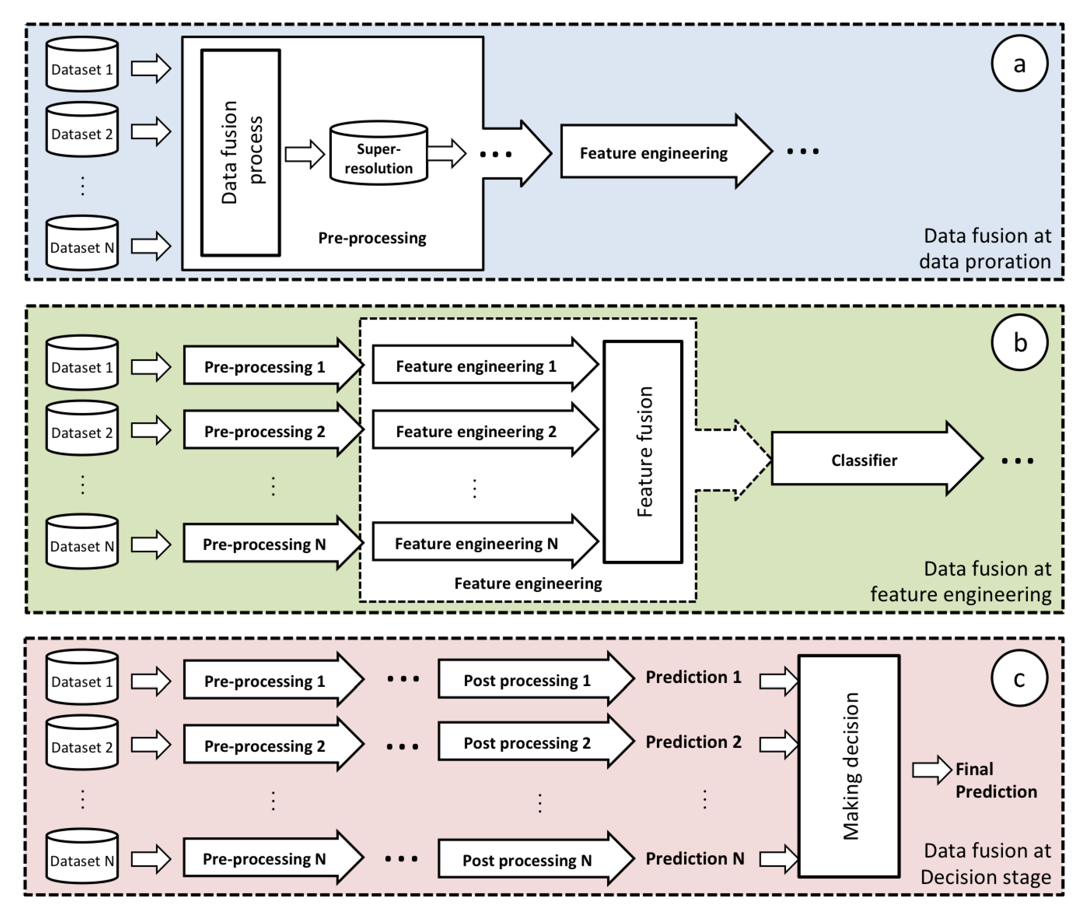
4.5. Multi-Modal Data Fusion

Data fusion is the process of combining data from multiple sources to improve the potential values and interpretation performance of the source data, and to produce a high-quality visible representation of the data [152]. In remote sensing, data fusion is commonly used to improve the spatial and spectral resolution of data. Although data fusion has a long history in the remote sensing community, the advent of machine learning and in particular deep learning techniques has dramatically changed the way the data are fused.
The initial step for any geo-data fusion is geo-coordinates matching. Then, having the paired data from the same scene, data fusion may take place in one of the following three stages: (1) at the data preparation stage, (2) at the feature engineering stage, or (3) at the decision stage (all shown in Figure 14).
Data fusion at the data preparation stage (also called Early Fusion) (Figure 14a) is usually referred to as super-resolution transformation. In this process, the aim is to increase the resolution of a targeted dataset by using another, sometimes temporary, source of data. A very traditional form of super-resolution transformation is pan-sharpening where the panchromatic data is employed to increase the resolution of MSI or HSI data. Different studies show that deep learning techniques outperform conventional pan-sharpening approaches by automatic extraction of features that indicate the correlations between the two data types [153,154,155,156].
Super-resolution generation using deep learning is obtained by a model in which two versions of an image (high resolution as the target and low resolution as the input) are used to learn how to reconstruct a higher resolution image out of a low resolution one [157,158,159]. These types of models are getting popular to increase the resolution of remote sensing data too [160,161]. In addition to the spatial resolution, the authors of [162] apply the same idea using 3D-CNNs on HSI to also provide higher spectral quality. By the launch of Sentinel 1 and Sentinel 2, many questions were raised regarding the fusion of SAR and MSI to increase the resolution of data in terms of filling the gaps caused by the atmospheric conditions. For instance, on a cloudy day, optical sensors can not capture the ground surface. To approach this problem, the authors of [163] propose a deep learning-based methodology using Sentinel 1 and Sentinel 2 time-series to estimate high-resolution NDVI time-series for monitoring agricultural changes. Another approach targeting the inner multi-modality of MSI data is by [164], wherein the proposed model super-resolves lower resolution spectral bands of Sentinel-2 data, using its higher resolution spectral bands.
Data fusion at the feature engineering stage (also called Feature/Representation Fusion) is a very common and efficient way of using multi-modal data. As also pictured in Figure 14b, instead of generating a new version of the input, the data sources from a scene are processed in parallel for the feature extraction. Then the extracted features of each pipeline are put together and fed to the classifier. Deep learning has been a breakthrough in this process. Using parallel convolutional streams, References [165,166] fuse LiDAR and MSI/HSI data at the feature engineering stage for the crop and land cover classification. Similarly, ref. [167] fuse SAR and MSI data to collect more ground details for classifications. Another interesting work belongs to [168], where the authors use OSM (Open Street Map) maps for semantic labelling of Earth Observation images. Panchromatic and MSI data are also commonly fused in many studies [169].
Another stage in which data fusion may take place is at the decision level (also called Late Fusion). As shown in Figure 14c, parallel streams leading to predictions are considered for each source of data, and the final decision is made based on all the streams’ predictions. Generally, the decision level data fusion stands out when the input data types and formats are not auto-correlated. Indeed, when the input data are heterogeneous, multi-modal, and multi-source at the same time, it is difficult to extract correlatable information at the earlier stages. Due to the large number of neurons in the architectures with data fusion at the decision stage, the required time to train, and hence to test the model, is significantly higher than the other data fusion architectures. Therefore, in the case of correlatable data types, as discussed in [167], the decision level data fusion is not the best approach. This is also stated in the work in [170], which compares the late fusion results with those of early fusion over aerial multispectral and LiDAR data and evaluates them with the same inference. On the other hand, a more heterogeneous input types situation has been explored by [171]: they adopt multi-modal (MSI and SAR), multi-source (aerial images, Sentinel 2 and Sentinel 1), and multi-temporal (for Sentinel 1 and 2) data types to rapidly extract flooded buildings.
Sometimes, data fusion targets the temporal resolution as well. The work in [172], published in 2018, is a review on the state-of-the-art of spatio-temporal multi-modal data fusion studies. In our review work, no study has been reported that tackles this problem using deep learning techniques. However, the authors predict a potential opening by emerging deep learning in the field.

4.6. Pre and Post-Processing

The aim of pre-processing is basically to enhance the raw input data for the analysis. Within this stage of the machine learning pipeline, many methodologies, as well as deep learning techniques, can be employed to generate an improved dataset from the raw data. As discussed earlier, data fusion can also happen during a pre-processing stage to generate super-resolution data. Furthermore, when pre-trained models on different datasets exist, transfer learning may also be considered within the data pre-processing stage. Also, the authors of [173] use transfer learning to overcome the problem of noises with the newly launched Chinese satellite hyperspectral images. Major pre-processing tasks given by the models in the literature focus on denoising, cloud detection, and resolution assessment. Besides data resolution assessment, deep learning has been also successful in HSI denoising [174,175], and in detecting clouds [176,177] for both MSI and HSI data.
Post-processing is an optional stage that is used to fine-tune the classifier output by usually employing image processing techniques. Based on prior knowledge about the expected output or about the potential classifier errors and noise, post-processing applies a set of adjustments to the output to enhance the model performance. In the context of remote sensing, the pre-processing stage is very useful to vectorise or create the shapefiles of on-Earth man-made objects (e.g., buildings) [170], for which the morphological characteristics of the expected output is known. Conditional random fields (CRFs) is the main technique used for this end [178], and it has been successfully practised by many studies jointly with deep learning models targeting semantically segmented maps [75,179,180].

5. Conclusions

Currently, the majority of the attempts to apply deep learning techniques on remote sensing data are proposed by non-machine learning experts. In this review, we addressed the critical challenges in employing such techniques and underlined the need for a deeper understating of machine learning as a complex problem. Focusing on the land use and land cover classification of multispectral and hyperspectral images, we provided a review on the state-of-the-art by converging a wide range of different approaches reported in the literature into a generic machine learning framework, which encompasses different aspects of the whole problem. We discussed how deep learning techniques have been utilised in different stages of the framework to target different tasks and challenges, standing out among the other approaches.
There is a growing interest in employing deep learning techniques for a wide spectrum of remote sensing applications, which encourages industries to invest in this field. Accordingly, fast developments in the ground knowledge and an increase in the number of open opportunities are expected. Going through the state-of-the-art, there seemed to be promising areas in which the implementation of deep learning can be of high potential:
  • For the majority of the commercially viable applications, the spatial resolution of remote sensing images is required to be higher than what any satellite can provide. Therefore, aerial remote sensing images are more popular due to their higher spatial resolution. Yet, the limited coverage and low temporal resolution of such aerial images come with some challenges for many applications that leave room for the use of satellite images as well. Therefore, the trade-off between temporal and spatial resolution lays the ground for further discussion on this matter.
  • The ground-truth scarcity is yet a challenge. An accurate annotated data set could open the doors to new opportunities for researchers. Most of the available solutions suffer from lack of funding and difficulty in assessment of their accuracy. Indeed, the use of IoT and the open science framework that supports the integration of citizen science, gamification, incentives and competitions, is still to be explored.
  • Despite the constant increase in the number of geospatial data providers, for many years there has been no standardised way to release and to get hold of the data. Commonly, processing and analysis of data are carried out on local machines, on the locally replicated instance of data. With the fast growth of data in volume and the limitation in memory, relying on conventional infrastructures appear not to be feasible and efficient anymore. Recently, data providers have introduced the cloud platform to access and analyse data directly, which offers the possibility of integration of data from different sources in the near future. Certainly, getting aligned with the advances in infrastructure opens up new opportunities to be investigated.
  • The recent idea of on-board data processing could introduce new challenges: as announced by NASA and ESA, the future satellites are planned to carry more powerful processors that can process data before transferring them to the Earth. However, the power-scale and energy management is a crucial problem for the on-board processes. Therefore, reducing the complexity of the models is a crucial matter to be considered for future works. The recent study by [181], which proposes the Firefly Harmony Search (FHS) tuning algorithm for its Deep Belief Network model, also proves that simplifying the models can also improve the accuracy of classifications.
Lastly, deep learning has an enormous capacity to act as an indispensable tool to tackle some of the most serious and urgent environmental concerns of our time. There is a sense of urgency to channel the direction of research activities to address such matters and there exist substantial potential scopes to be further developed in this area. Moreover, the effective use of deep learning deliberates new case studies and requires determined efforts to tackle the technical challenges that come with remote sensing data and the problem of resource-constrained machines. Memory management, data preparation, and data loading are of these technical challenges that call for further endeavours in applications of deep learning. Furthermore, deep learning studies in the field of remote sensing lack an established framework that can categorise and optimally group the models. Future efforts may consider the need for setting up such a framework that can set the ground for a rational and proper assessment of the effectiveness of the models.

Author Contributions

Conceptualization, A.V., S.C. and M.M.; methodology, A.V., S.C. and M.M.; investigation, A.V.; resources, S.C. and M.M.; data curation, A.V.; writing—original draft preparation, A.V.; writing—review and editing, S.C. and M.M.; visualization, A.V.; supervision, S.C. and M.M. All authors have read and agreed to the published version of the manuscript.

Funding

This research received no external funding.

Conflicts of Interest

The authors declare no conflict of interest.

References

  1. ESA. Towards a European AI4EO R&I Agenda. 2018. Available online: https://eo4society.esa.int/wp-content/uploads/2018/09/ai4eo_v1.0.pdf (accessed on 15 January 2019).
  2. Newbold, T.; Hudson, L.N.; Hill, S.L.; Contu, S.; Lysenko, I.; Senior, R.A.; Börger, L.; Bennett, D.J.; Choimes, A.; Collen, B.; et al. Global effects of land use on local terrestrial biodiversity. Nature 2015, 520, 45. [Google Scholar] [CrossRef] [Green Version]
  3. Vitousek, P.M.; Mooney, H.A.; Lubchenco, J.; Melillo, J.M. Human domination of Earth’s ecosystems. Science 1997, 277, 494–499. [Google Scholar] [CrossRef] [Green Version]
  4. Feddema, J.J.; Oleson, K.W.; Bonan, G.B.; Mearns, L.O.; Buja, L.E.; Meehl, G.A.; Washington, W.M. The importance of land-cover change in simulating future climates. Science 2005, 310, 1674–1678. [Google Scholar] [CrossRef] [Green Version]
  5. Turner, B.L.; Moss, R.H.; Skole, D. Relating Land Use and Global Land-Cover Change; IGBP Report 24, HDP Report 5; IGDP Report No. 24; HDP Report No. 5; International Geosphere-Biosphere Programme: Stockholm, Sweden, 1993. [Google Scholar]
  6. United Nations Office for Disaster Risk Reduction. Sendai framework for disaster risk reduction 2015–2030. In Proceedings of the 3rd United Nations World Conference on Disaster Risk Reduction (WCDRR), Sendai, Japan, 14–18 March 2015; pp. 14–18. [Google Scholar]
  7. Zikopoulos, P.; Eaton, C. Understanding Big Data: Analytics for Enterprise Class Hadoop and Streaming Data; McGraw-Hill Osborne Media: New York, NY, USA, 2011. [Google Scholar]
  8. Zhu, X.X.; Tuia, D.; Mou, L.; Xia, G.S.; Zhang, L.; Xu, F.; Fraundorfer, F. Deep learning in remote sensing: A comprehensive review and list of resources. IEEE Geosci. Remote Sens. Mag. 2017, 5, 8–36. [Google Scholar] [CrossRef] [Green Version]
  9. Fisher, P.; Comber, A.J.; Wadsworth, R. Land use and land cover: Contradiction or complement. In Re-Presenting GIS; Wiley: New York, NY, USA, 2005; pp. 85–98. [Google Scholar]
  10. Food and Agriculture Organization of the United Nations. 2019. Available online: http://www.fao.org/faostat (accessed on 29 July 2020).
  11. Di Gregorio, A. Land Cover Classification System: Classification Concepts and User Manual: LCCS; Food & Agriculture Org.: Rome, Italy, 2005; Volume 2. [Google Scholar]
  12. Isikdogan, F.; Bovik, A.C.; Passalacqua, P. Surface water mapping by deep learning. IEEE J. Sel. Top. Appl. Earth Obs. Remote Sens. 2017, 10, 4909–4918. [Google Scholar] [CrossRef]
  13. Rezaee, M.; Mahdianpari, M.; Zhang, Y.; Salehi, B. Deep convolutional neural network for complex wetland classification using optical remote sensing imagery. IEEE J. Sel. Top. Appl. Earth Obs. Remote Sens. 2018, 11, 3030–3039. [Google Scholar] [CrossRef]
  14. Huang, B.; Zhao, B.; Song, Y. Urban land-use mapping using a deep convolutional neural network with high spatial resolution multispectral remote sensing imagery. Remote Sens. Environ. 2018, 214, 73–86. [Google Scholar] [CrossRef]
  15. Hu, J.; Mou, L.; Schmitt, A.; Zhu, X.X. FusioNet: A two-stream convolutional neural network for urban scene classification using PolSAR and hyperspectral data. In Proceedings of the 2017 Joint Urban Remote Sensing Event (JURSE), Dubai, UAE, 6–8 March 2017; pp. 1–4. [Google Scholar]
  16. Kussul, N.; Lavreniuk, M.; Skakun, S.; Shelestov, A. Deep learning classification of land cover and crop types using remote sensing data. IEEE Geosci. Remote Sens. Lett. 2017, 14, 778–782. [Google Scholar] [CrossRef]
  17. Awad, M.; Jomaa, I.; Arab, F. Improved capability in stone pine forest mapping and management in Lebanon using hyperspectral CHRIS-Proba data relative to Landsat ETM+. Photogramm. Eng. Remote Sens. 2014, 80, 725–731. [Google Scholar] [CrossRef]
  18. Marschner, F. Major Land Uses in the United States (Map Scale 1:5,000,000); USDA Agricultural Research Service: Washington, DC, USA, 1950; Volume 252.
  19. Anderson, J.R. A Land Use and Land Cover Classification System for Use with Remote Sensor Data; US Government Printing Office: Washington, DC, USA, 1976; Volume 964.
  20. Cowardin, L.M.; Carter, V.; Golet, F.C.; LaRoe, E.T. Classification of Wetlands and Deepwater Habitats of the United States; Technical Report; US Department of the Interior, US Fish and Wildlife Service: Washington, DC, USA, 1979.
  21. Pohl, C.; Van Genderen, J.L. Review article multisensor image fusion in remote sensing: Concepts, methods and applications. Int. J. Remote Sens. 1998, 19, 823–854. [Google Scholar] [CrossRef] [Green Version]
  22. Congalton, R.G. A review of assessing the accuracy of classifications of remotely sensed data. Remote Sens. Environ. 1991, 37, 35–46. [Google Scholar] [CrossRef]
  23. Singh, A. Review article digital change detection techniques using remotely-sensed data. Int. J. Remote Sens. 1989, 10, 989–1003. [Google Scholar] [CrossRef] [Green Version]
  24. Kasischke, E.S.; Melack, J.M.; Dobson, M.C. The use of imaging radars for ecological applications—A review. Remote Sens. Environ. 1997, 59, 141–156. [Google Scholar] [CrossRef]
  25. Li, S.; Kang, X.; Fang, L.; Hu, J.; Yin, H. Pixel-level image fusion: A survey of the state of the art. Inf. Fusion 2017, 33, 100–112. [Google Scholar] [CrossRef]
  26. Ma, L.; Liu, Y.; Zhang, X.; Ye, Y.; Yin, G.; Johnson, B.A. Deep learning in remote sensing applications: A meta-analysis and review. ISPRS J. Photogramm. Remote Sens. 2019, 152, 166–177. [Google Scholar] [CrossRef]
  27. Deng, J.; Dong, W.; Socher, R.; Li, L.J.; Li, K.; Fei-Fei, L. Imagenet: A large-scale hierarchical image database. In Proceedings of the 2009 IEEE Conference on Computer Vision and Pattern Recognition, Miami, FL, USA, 20–25 June 2009; pp. 248–255. [Google Scholar]
  28. Paoletti, M.; Haut, J.; Plaza, J.; Plaza, A. Deep learning classifiers for hyperspectral imaging: A review. ISPRS J. Photogramm. Remote Sens. 2019, 158, 279–317. [Google Scholar] [CrossRef]
  29. Li, S.; Song, W.; Fang, L.; Chen, Y.; Ghamisi, P.; Benediktsson, J.A. Deep learning for hyperspectral image classification: An overview. IEEE Trans. Geosci. Remote Sens. 2019, 57, 6690–6709. [Google Scholar] [CrossRef] [Green Version]
  30. Goetz, A.F. Three decades of hyperspectral remote sensing of the Earth: A personal view. Remote Sens. Environ. 2009, 113, S5–S16. [Google Scholar] [CrossRef]
  31. Ghamisi, P.; Maggiori, E.; Li, S.; Souza, R.; Tarablaka, Y.; Moser, G.; De Giorgi, A.; Fang, L.; Chen, Y.; Chi, M.; et al. New frontiers in spectral-spatial hyperspectral image classification: The latest advances based on mathematical morphology, Markov random fields, segmentation, sparse representation, and deep learning. IEEE Geosci. Remote Sens. Mag. 2018, 6, 10–43. [Google Scholar] [CrossRef]
  32. Imani, M.; Ghassemian, H. An overview on spectral and spatial information fusion for hyperspectral image classification: Current trends and challenges. Inf. Fusion 2020, 59, 59–83. [Google Scholar] [CrossRef]
  33. USGS. USGS Earth Explorer. 2019. Available online: https://earthexplorer.usgs.gov/ (accessed on 29 July 2020).
  34. USGS. USGS Global Visualization Viewer. 2019. Available online: https://glovis.usgs.gov/app (accessed on 29 July 2020).
  35. NASA. NASA Earth Observation—NEO. 2019. Available online: https://neo.sci.gsfc.nasa.gov/ (accessed on 29 July 2020).
  36. ESA. The Copernicus Open Access Hub. 2019. Available online: https://scihub.copernicus.eu/dhus/ (accessed on 29 July 2020).
  37. NASA. NASA Earth Data Search. 2019. Available online: https://search.earthdata.nasa.gov/search (accessed on 29 July 2020).
  38. NOAA. NOAA Data Access. 2019. Available online: https://www.ncdc.noaa.gov/data-access (accessed on 29 July 2020).
  39. NOAA. NOAA Digital Coast. 2019. Available online: https://coast.noaa.gov/digitalcoast/ (accessed on 29 July 2020).
  40. IPUMS. IPUMS Terra Integrates Population and Environmental Data. 2018. Available online: https://terra.ipums.org/ (accessed on 29 July 2020).
  41. Penatti, O.A.; Nogueira, K.; Dos Santos, J.A. Do deep features generalize from everyday objects to remote sensing and aerial scenes domains? In Proceedings of the IEEE conference on computer vision and pattern recognition workshops (CVPR), Boston, MA, USA, 7–12 June 2015; pp. 44–51. [Google Scholar]
  42. Demir, I.; Koperski, K.; Lindenbaum, D.; Pang, G.; Huang, J.; Basu, S.; Hughes, F.; Tuia, D.; Raska, R. Deepglobe 2018: A challenge to parse the earth through satellite images. In Proceedings of the 2018 IEEE/CVF Conference on Computer Vision and Pattern Recognition Workshops (CVPRW), Salt Lake City, UT, USA, 18–22 June 2018; pp. 172–17209. [Google Scholar]
  43. Basu, S.; Ganguly, S.; Mukhopadhyay, S.; DiBiano, R.; Karki, M.; Nemani, R. Deepsat: A learning framework for satellite imagery. In Proceedings of the 23rd SIGSPATIAL International Conference on Advances in Geographic Information Systems, Washington, DC, USA, 3–6 November 2015; p. 37. [Google Scholar]
  44. Yang, Y.; Newsam, S. Bag-of-visual-words and spatial extensions for land-use classification. In Proceedings of the 18th SIGSPATIAL International Conference on Advances in Geographic Information Systems, San Jose, CA, USA, 2–5 November 2010; pp. 270–279. [Google Scholar]
  45. GIC. Hyperspectral Remote Sensing Scenes. 2020. Available online: http://www.ehu.eus/ccwintco/index.php/Hyperspectral_Remote_Sensing_Scenes (accessed on 29 July 2020).
  46. Geoscience. 2013 IEEE GRSS Data Fusion Contest; GRSS: Piscataway, NJ, USA, 2013. [Google Scholar]
  47. Codalab. DeepGlobe Land Cover Classification Challenge; DeepGlobe: Salt Lake City, UT, USA, 2018. [Google Scholar]
  48. Basu, S. SAT-4 and SAT-6 Airborne Datasets; Louisiana State University: Baton Rouge, LA, USA, 2015. [Google Scholar]
  49. University of California, Merced. UC Merced Land Use Dataset; University of California, Merced: Merced, CA, USA, 2010. [Google Scholar]
  50. Patrero. Brazilian Coffee Scenes Dataset; Patrero: San Francisco, CA, USA, 2015. [Google Scholar]
  51. System(EOS). Crop Monitoring. 2020. Available online: https://eos.com/eos-crop-monitoring/ (accessed on 29 July 2020).
  52. Awad, M.M.; Alawar, B.; Jbeily, R. A new crop spectral signatures database interactive tool (CSSIT). Data 2019, 4, 77. [Google Scholar] [CrossRef] [Green Version]
  53. Global Forest Watch. Developer Tools. 2020. Available online: https://developers.globalforestwatch.org/ (accessed on 29 July 2020).
  54. SERVIR-Mekong. Surface Water Mapping Tool. 2020. Available online: http://surface-water-servir.adpc.net/ (accessed on 29 July 2020).
  55. Wolpert, D.H. The lack of a priori distinctions between learning algorithms. Neural Comput. 1996, 8, 1341–1390. [Google Scholar] [CrossRef]
  56. Wolpert, D.H.; Macready, W.G. Coevolutionary free lunches. IEEE Trans. Evol. Comput. 2005, 9, 721–735. [Google Scholar] [CrossRef]
  57. Zhang, C.; Bengio, S.; Hardt, M.; Recht, B.; Vinyals, O. Understanding deep learning requires rethinking generalization. arXiv 2016, arXiv:1611.03530. [Google Scholar]
  58. Kawaguchi, K.; Kaelbling, L.P.; Bengio, Y. Generalization in deep learning. arXiv 2017, arXiv:1710.05468. [Google Scholar]
  59. Saxe, A.M.; Bansal, Y.; Dapello, J.; Advani, M.; Kolchinsky, A.; Tracey, B.D.; Cox, D.D. On the information bottleneck theory of deep learning. J. Stat. Mech. Theory Exp. 2019, 2019, 124020. [Google Scholar] [CrossRef]
  60. Dinh, L.; Pascanu, R.; Bengio, S.; Bengio, Y. Sharp minima can generalize for deep nets. In Proceedings of the 34th International Conference on Machine Learning (ICML), Sydney, Australia, 10–15 July 2017; pp. 1019–1028. [Google Scholar]
  61. Zou, Q.; Ni, L.; Zhang, T.; Wang, Q. Deep learning based feature selection for remote sensing scene classification. IEEE Geosci. Remote Sens. Lett. 2015, 12, 2321–2325. [Google Scholar] [CrossRef]
  62. Han, W.; Feng, R.; Wang, L.; Cheng, Y. A semi-supervised generative framework with deep learning features for high-resolution remote sensing image scene classification. ISPRS J. Photogramm. Remote Sens. 2018, 145, 23–43. [Google Scholar] [CrossRef]
  63. IBM. Removing the Hunch in Data Science with AI-Based Automated Feature Engineering. 2017. Available online: https://www.ibm.com/blogs/research/2017/08/ai-based-automated-feature-engineering/ (accessed on 29 July 2020).
  64. Zhang, L.; Zhang, L.; Tao, D.; Huang, X. Tensor discriminative locality alignment for hyperspectral image spectral–spatial feature extraction. IEEE Trans. Geosci. Remote Sens. 2012, 51, 242–256. [Google Scholar] [CrossRef]
  65. Hughes, G. On the mean accuracy of statistical pattern recognizers. IEEE Trans. Inf. Theory 1968, 14, 55–63. [Google Scholar] [CrossRef] [Green Version]
  66. Rasti, B.; Hong, D.; Hang, R.; Ghamisi, P.; Kang, X.; Chanussot, J.; Benediktsson, J.A. Feature extraction for hyperspectral imagery: The evolution from shallow to deep. arXiv 2020, arXiv:2003.02822. [Google Scholar]
  67. Yu, S.; Jia, S.; Xu, C. Convolutional neural networks for hyperspectral image classification. Neurocomputing 2017, 219, 88–98. [Google Scholar] [CrossRef]
  68. Sun, W.; Du, Q. Graph-regularized fast and robust principal component analysis for hyperspectral band selection. IEEE Trans. Geosci. Remote Sens. 2018, 56, 3185–3195. [Google Scholar] [CrossRef]
  69. Zabalza, J.; Ren, J.; Ren, J.; Liu, Z.; Marshall, S. Structured covariance principal component analysis for real-time onsite feature extraction and dimensionality reduction in hyperspectral imaging. Appl. Opt. 2014, 53, 4440–4449. [Google Scholar] [CrossRef] [PubMed] [Green Version]
  70. Chen, S.; Zhang, D. Semisupervised dimensionality reduction with pairwise constraints for hyperspectral image classification. IEEE Geosci. Remote Sens. Lett. 2010, 8, 369–373. [Google Scholar] [CrossRef]
  71. Archibald, R.; Fann, G. Feature selection and classification of hyperspectral images with support vector machines. IEEE Geosci. Remote Sens. Lett. 2007, 4, 674–677. [Google Scholar] [CrossRef]
  72. Kuo, B.C.; Ho, H.H.; Li, C.H.; Hung, C.C.; Taur, J.S. A kernel-based feature selection method for SVM with RBF kernel for hyperspectral image classification. IEEE J. Sel. Top. Appl. Earth Obs. Remote Sens. 2013, 7, 317–326. [Google Scholar]
  73. Zhong, Z.; Li, J.; Luo, Z.; Chapman, M. Spectral–spatial residual network for hyperspectral image classification: A 3-D deep learning framework. IEEE Trans. Geosci. Remote Sens. 2017, 56, 847–858. [Google Scholar] [CrossRef]
  74. Mou, L.; Ghamisi, P.; Zhu, X.X. Unsupervised spectral–spatial feature learning via deep residual Conv–Deconv network for hyperspectral image classification. IEEE Trans. Geosci. Remote Sens. 2017, 56, 391–406. [Google Scholar] [CrossRef] [Green Version]
  75. Audebert, N.; Le Saux, B.; Lefèvre, S. Semantic segmentation of earth observation data using multimodal and multi-scale deep networks. In Proceedings of the Asian Conference on Computer Vision (ACCV), Taipei, Taiwan, 20–24 November 2016; pp. 180–196. [Google Scholar]
  76. Tao, C.; Pan, H.; Li, Y.; Zou, Z. Unsupervised spectral–spatial feature learning with stacked sparse autoencoder for hyperspectral imagery classification. IEEE Geosci. Remote Sens. Lett. 2015, 12, 2438–2442. [Google Scholar]
  77. Ma, X.; Wang, H.; Geng, J. Spectral–spatial classification of hyperspectral image based on deep auto-encoder. IEEE J. Sel. Top. Appl. Earth Obs. Remote Sens. 2016, 9, 4073–4085. [Google Scholar] [CrossRef]
  78. Zabalza, J.; Ren, J.; Zheng, J.; Zhao, H.; Qing, C.; Yang, Z.; Du, P.; Marshall, S. Novel segmented stacked autoencoder for effective dimensionality reduction and feature extraction in hyperspectral imaging. Neurocomputing 2016, 185, 1–10. [Google Scholar] [CrossRef] [Green Version]
  79. Lunga, D.; Prasad, S.; Crawford, M.M.; Ersoy, O. Manifold-learning-based feature extraction for classification of hyperspectral data: A review of advances in manifold learning. IEEE Signal Process. Mag. 2013, 31, 55–66. [Google Scholar] [CrossRef]
  80. Zhao, W.; Du, S. Spectral–spatial feature extraction for hyperspectral image classification: A dimension reduction and deep learning approach. IEEE Trans. Geosci. Remote Sens. 2016, 54, 4544–4554. [Google Scholar] [CrossRef]
  81. Shi, Q.; Zhang, L.; Du, B. Semisupervised discriminative locally enhanced alignment for hyperspectral image classification. IEEE Trans. Geosci. Remote Sens. 2013, 51, 4800–4815. [Google Scholar] [CrossRef]
  82. Li, W.; Prasad, S.; Fowler, J.E.; Bruce, L.M. Locality-preserving dimensionality reduction and classification for hyperspectral image analysis. IEEE Trans. Geosci. Remote Sens. 2011, 50, 1185–1198. [Google Scholar] [CrossRef] [Green Version]
  83. Prasad, S.; Bruce, L.M. Limitations of principal components analysis for hyperspectral target recognition. IEEE Geosci. Remote Sens. Lett. 2008, 5, 625–629. [Google Scholar] [CrossRef]
  84. Wang, Q.; Meng, Z.; Li, X. Locality adaptive discriminant analysis for spectral–spatial classification of hyperspectral images. IEEE Geosci. Remote Sens. Lett. 2017, 14, 2077–2081. [Google Scholar] [CrossRef]
  85. Zhou, Y.; Peng, J.; Chen, C.P. Dimension reduction using spatial and spectral regularized local discriminant embedding for hyperspectral image classification. IEEE Trans. Geosci. Remote Sens. 2014, 53, 1082–1095. [Google Scholar] [CrossRef]
  86. Breiman, L. Bagging predictors. Mach. Learn. 1996, 24, 123–140. [Google Scholar] [CrossRef] [Green Version]
  87. Breiman, L. Random forests. Mach. Learn. 2001, 45, 5–32. [Google Scholar] [CrossRef] [Green Version]
  88. Pal, M. Random forest classifier for remote sensing classification. Int. J. Remote Sens. 2005, 26, 217–222. [Google Scholar] [CrossRef]
  89. Colditz, R. An evaluation of different training sample allocation schemes for discrete and continuous land cover classification using decision tree-based algorithms. Remote Sens. 2015, 7, 9655–9681. [Google Scholar] [CrossRef] [Green Version]
  90. Stefanski, J.; Mack, B.; Waske, B. Optimization of object-based image analysis with random forests for land cover mapping. IEEE J. Sel. Top. Appl. Earth Obs. Remote Sens. 2013, 6, 2492–2504. [Google Scholar] [CrossRef]
  91. Belgiu, M.; Drăguţ, L. Random forest in remote sensing: A review of applications and future directions. ISPRS J. Photogramm. Remote Sens. 2016, 114, 24–31. [Google Scholar] [CrossRef]
  92. Mountrakis, G.; Im, J.; Ogole, C. Support vector machines in remote sensing: A review. ISPRS J. Photogramm. Remote Sens. 2011, 66, 247–259. [Google Scholar] [CrossRef]
  93. Cawley, G.C.; Talbot, N.L. Preventing over-fitting during model selection via Bayesian regularisation of the hyper-parameters. J. Mach. Learn. Res. 2007, 8, 841–861. [Google Scholar]
  94. Cawley, G.C.; Talbot, N.L. On over-fitting in model selection and subsequent selection bias in performance evaluation. J. Mach. Learn. Res. 2010, 11, 2079–2107. [Google Scholar]
  95. Melgani, F.; Bruzzone, L. Classification of hyperspectral remote sensing images with support vector machines. IEEE Trans. Geosci. Remote Sens. 2004, 42, 1778–1790. [Google Scholar] [CrossRef] [Green Version]
  96. Fauvel, M.; Chanussot, J.; Benediktsson, J.A.; Sveinsson, J.R. Spectral and spatial classification of hyperspectral data using SVMs and morphological profiles. In Proceedings of the 2007 IEEE International Geoscience and Remote Sensing Symposium (IGARSS2007), Barcelona, Spain, 23–27 July 2007; pp. 4834–4837. [Google Scholar]
  97. Mitra, P.; Shankar, B.U.; Pal, S.K. Segmentation of multispectral remote sensing images using active support vector machines. Pattern Recognit. Lett. 2004, 25, 1067–1074. [Google Scholar] [CrossRef]
  98. LeCun, Y.; Bengio, Y.; Hinton, G. Deep learning. Nature 2015, 521, 436. [Google Scholar] [CrossRef] [PubMed]
  99. Zhang, H.; Li, Y.; Zhang, Y.; Shen, Q. Spectral-spatial classification of hyperspectral imagery using a dual-channel convolutional neural network. Remote Sens. Lett. 2017, 8, 438–447. [Google Scholar] [CrossRef] [Green Version]
  100. Mou, L.; Ghamisi, P.; Zhu, X.X. Fully conv-deconv network for unsupervised spectral-spatial feature extraction of hyperspectral imagery via residual learning. In Proceedings of the 2017 IEEE International Geoscience and Remote Sensing Symposium (IGARSS), Fort Worth, TX, USA, 23–28 July 2017; pp. 5181–5184. [Google Scholar]
  101. Hu, W.; Huang, Y.; Wei, L.; Zhang, F.; Li, H. Deep convolutional neural networks for hyperspectral image classification. J. Sens. 2015, 2015, 12. [Google Scholar] [CrossRef] [Green Version]
  102. Guidici, D.; Clark, M. One-Dimensional convolutional neural network land-cover classification of multi-seasonal hyperspectral imagery in the San Francisco Bay Area, California. Remote Sens. 2017, 9, 629. [Google Scholar] [CrossRef] [Green Version]
  103. Wu, H.; Prasad, S. Convolutional recurrent neural networks for hyperspectral data classification. Remote Sens. 2017, 9, 298. [Google Scholar] [CrossRef] [Green Version]
  104. Zhu, L.; Chen, Y.; Ghamisi, P.; Benediktsson, J.A. Generative adversarial networks for hyperspectral image classification. IEEE Trans. Geosci. Remote Sens. 2018, 56, 5046–5063. [Google Scholar] [CrossRef]
  105. Zhang, L.; Zhang, L.; Du, B. Deep learning for remote sensing data: A technical tutorial on the state of the art. IEEE Geosci. Remote Sens. Mag. 2016, 4, 22–40. [Google Scholar] [CrossRef]
  106. LeCun, Y.; Bottou, L.; Bengio, Y.; Haffner, P. Gradient-based learning applied to document recognition. Proc. IEEE 1998, 86, 2278–2324. [Google Scholar] [CrossRef] [Green Version]
  107. Krizhevsky, A.; Sutskever, I.; Hinton, G.E. Imagenet classification with deep convolutional neural networks. In Advances in Neural Information Processing Systems (NIPS); ACM: New York, NY, USA, 2012; pp. 1097–1105. [Google Scholar]
  108. Simonyan, K.; Zisserman, A. Very deep convolutional networks for large-scale image recognition. In Proceedings of the ICLR 2015, San Diego, CA, USA, 7–9 May 2015. [Google Scholar]
  109. Jia, Y.; Shelhamer, E.; Donahue, J.; Karayev, S.; Long, J.; Girshick, R.; Guadarrama, S.; Darrell, T. Caffe: Convolutional architecture for fast feature embedding. In Proceedings of the 22nd ACM international conference on Multimedia, Orlando, FL, USA, 3–7 November 2014; pp. 675–678. [Google Scholar]
  110. Szegedy, C.; Liu, W.; Jia, Y.; Sermanet, P.; Reed, S.; Anguelov, D.; Erhan, D.; Vanhoucke, V.; Rabinovich, A. Going deeper with convolutions. In Proceedings of the IEEE conference on computer vision and pattern recognition (CVPR), Boston, MA, USA, 7–12 June 2015; pp. 1–9. [Google Scholar]
  111. He, K.; Zhang, X.; Ren, S.; Sun, J. Deep residual learning for image recognition. In Proceedings of the IEEE conference on computer vision and pattern recognition (CVPR), Las Vegas, NV, USA, 27–30 June 2016; pp. 770–778. [Google Scholar]
  112. Nogueira, K.; Penatti, O.A.; dos Santos, J.A. Towards better exploiting convolutional neural networks for remote sensing scene classification. Pattern Recognit. 2017, 61, 539–556. [Google Scholar] [CrossRef] [Green Version]
  113. Ji, S.; Zhang, C.; Xu, A.; Shi, Y.; Duan, Y. 3D convolutional neural networks for crop classification with multi-temporal remote sensing images. Remote Sens. 2018, 10, 75. [Google Scholar] [CrossRef] [Green Version]
  114. Li, Y.; Zhang, H.; Shen, Q. Spectral–spatial classification of hyperspectral imagery with 3D convolutional neural network. Remote Sens. 2017, 9, 67. [Google Scholar] [CrossRef] [Green Version]
  115. Chen, Y.; Jiang, H.; Li, C.; Jia, X.; Ghamisi, P. Deep feature extraction and classification of hyperspectral images based on convolutional neural networks. IEEE Trans. Geosci. Remote Sens. 2016, 54, 6232–6251. [Google Scholar] [CrossRef] [Green Version]
  116. Sun, H.; Zheng, X.; Lu, X.; Wu, S. Spectral-Spatial Attention Network for Hyperspectral Image Classification. IEEE Trans. Geosci. Remote Sens. 2019. [Google Scholar] [CrossRef]
  117. Lin, M.; Chen, Q.; Yan, S. Network in network. arXiv 2013, arXiv:1312.4400. [Google Scholar]
  118. Hu, Y.; Zhang, Q.; Zhang, Y.; Yan, H. A Deep Convolution Neural Network Method for Land Cover Mapping: A Case Study of Qinhuangdao, China. Remote Sens. 2018, 10, 2053. [Google Scholar] [CrossRef] [Green Version]
  119. Castelluccio, M.; Poggi, G.; Sansone, C.; Verdoliva, L. Land use classification in remote sensing images by convolutional neural networks. arXiv 2015, arXiv:1508.00092. [Google Scholar]
  120. Scott, G.J.; England, M.R.; Starms, W.A.; Marcum, R.A.; Davis, C.H. Training deep convolutional neural networks for land–cover classification of high-resolution imagery. IEEE Geosci. Remote Sens. Lett. 2017, 14, 549–553. [Google Scholar] [CrossRef]
  121. Cheng, G.; Han, J.; Lu, X. Remote sensing image scene classification: Benchmark and state of the art. Proc. IEEE 2017, 105, 1865–1883. [Google Scholar] [CrossRef] [Green Version]
  122. Helber, P.; Bischke, B.; Dengel, A.; Borth, D. Eurosat: A novel dataset and deep learning benchmark for land use and land cover classification. IEEE J. Sel. Top. Appl. Earth Obs. Remote Sens. 2019. [Google Scholar] [CrossRef] [Green Version]
  123. Lee, H.; Kwon, H. Going deeper with contextual CNN for hyperspectral image classification. IEEE Trans. Image Process. 2017, 26, 4843–4855. [Google Scholar] [CrossRef] [Green Version]
  124. Mahdianpari, M.; Salehi, B.; Rezaee, M.; Mohammadimanesh, F.; Zhang, Y. Very deep convolutional neural networks for complex land cover mapping using multispectral remote sensing imagery. Remote Sens. 2018, 10, 1119. [Google Scholar] [CrossRef] [Green Version]
  125. Wang, Q.; Liu, S.; Chanussot, J.; Li, X. Scene classification with recurrent attention of VHR remote sensing images. IEEE Trans. Geosci. Remote Sens. 2018, 57, 1155–1167. [Google Scholar] [CrossRef]
  126. Ronneberger, O.; Fischer, P.; Brox, T. U-net: Convolutional networks for biomedical image segmentation. In Proceedings of the International Conference on Medical image computing and computer-assisted intervention (MICCAI), Munich, Germany, 5–9 October 2015; pp. 234–241. [Google Scholar]
  127. Xu, Y.; Wu, L.; Xie, Z.; Chen, Z. Building extraction in very high resolution remote sensing imagery using deep learning and guided filters. Remote Sens. 2018, 10, 144. [Google Scholar] [CrossRef] [Green Version]
  128. Hamaguchi, R.; Fujita, A.; Nemoto, K.; Imaizumi, T.; Hikosaka, S. Effective use of dilated convolutions for segmenting small object instances in remote sensing imagery. In Proceedings of the 2018 IEEE Winter Conference on Applications of Computer Vision (WACV), Lake Tahoe, NV, USA, 12–15 March 2018; pp. 1442–1450. [Google Scholar]
  129. Zhang, Z.; Liu, Q.; Wang, Y. Road extraction by deep residual u-net. IEEE Geosci. Remote Sens. Lett. 2018, 15, 749–753. [Google Scholar] [CrossRef] [Green Version]
  130. Shi, Q.; Liu, X.; Li, X. Road detection from remote sensing images by generative adversarial networks. IEEE Access 2017, 6, 25486–25494. [Google Scholar] [CrossRef]
  131. Mohajerani, S.; Krammer, T.A.; Saeedi, P. Cloud Detection Algorithm for Remote Sensing Images Using Fully Convolutional Neural Networks. arXiv 2018, arXiv:1810.05782. [Google Scholar]
  132. Zhang, Z.; Iwasaki, A.; Xu, G.; Song, J. Cloud detection on small satellites based on lightweight U-net and image compression. J. Appl. Remote Sens. 2019, 13, 026502. [Google Scholar] [CrossRef]
  133. Li, R.; Liu, W.; Yang, L.; Sun, S.; Hu, W.; Zhang, F.; Li, W. DeepUNet: A deep fully convolutional network for pixel-level sea-land segmentation. IEEE J. Sel. Top. Appl. Earth Obs. Remote Sens. 2018, 11, 3954–3962. [Google Scholar] [CrossRef] [Green Version]
  134. Papadomanolaki, M.; Vakalopoulou, M.; Karantzalos, K. A Novel Object-Based Deep Learning Framework for Semantic Segmentation of Very High-Resolution Remote Sensing Data: Comparison with Convolutional and Fully Convolutional Networks. Remote Sens. 2019, 11, 684. [Google Scholar] [CrossRef] [Green Version]
  135. Rakhlin, A.; Davydow, A.; Nikolenko, S.I. Land Cover Classification From Satellite Imagery With U-Net and Lovasz-Softmax Loss. In Proceedings of the 2018 IEEE/CVF Conference on Computer Vision and Pattern Recognition Workshops (CVPRW), Salt Lake City, UT, USA, 18–22 June 2018; pp. 262–266. [Google Scholar]
  136. Shrestha, A.; Mahmood, A. Review of deep learning algorithms and architectures. IEEE Access 2019, 7, 53040–53065. [Google Scholar] [CrossRef]
  137. Liu, P.; Choo, K.K.R.; Wang, L.; Huang, F. SVM or deep learning? A comparative study on remote sensing image classification. Soft Comput. 2017, 21, 7053–7065. [Google Scholar] [CrossRef]
  138. Yu, X.; Wu, X.; Luo, C.; Ren, P. Deep learning in remote sensing scene classification: A data augmentation enhanced convolutional neural network framework. GIScience Remote Sens. 2017, 54, 741–758. [Google Scholar] [CrossRef] [Green Version]
  139. Triguero, I.; García, S.; Herrera, F. Self-labeled techniques for semi-supervised learning: Taxonomy, software and empirical study. Knowl. Inf. Syst. 2015, 42, 245–284. [Google Scholar] [CrossRef]
  140. Torrey, L.; Shavlik, J. Transfer learning. In Handbook of Research on Machine Learning Applications and Trends: Algorithms, Methods, and Techniques; IGI Global: Hershey, PA, USA, 2010; pp. 242–264. [Google Scholar]
  141. Marmanis, D.; Datcu, M.; Esch, T.; Stilla, U. Deep learning earth observation classification using ImageNet pretrained networks. IEEE Geosci. Remote Sens. Lett. 2015, 13, 105–109. [Google Scholar] [CrossRef] [Green Version]
  142. Zhou, W.; Newsam, S.; Li, C.; Shao, Z. Learning low dimensional convolutional neural networks for high-resolution remote sensing image retrieval. Remote Sens. 2017, 9, 489. [Google Scholar] [CrossRef] [Green Version]
  143. Chen, Z.; Zhang, T.; Ouyang, C. End-to-end airplane detection using transfer learning in remote sensing images. Remote Sens. 2018, 10, 139. [Google Scholar] [CrossRef] [Green Version]
  144. Hong, D.; Yokoya, N.; Xia, G.S.; Chanussot, J.; Zhu, X.X. X-ModalNet: A semi-supervised deep cross-modal network for classification of remote sensing data. ISPRS J. Photogramm. Remote Sens. 2020, 167, 12–23. [Google Scholar] [CrossRef]
  145. Nalepa, J.; Myller, M.; Imai, Y.; Honda, K.i.; Takeda, T.; Antoniak, M. Unsupervised Segmentation of Hyperspectral Images Using 3D Convolutional Autoencoders. arXiv 2019, arXiv:1907.08870. [Google Scholar]
  146. Guo, X.; Liu, X.; Zhu, E.; Yin, J. Deep clustering with convolutional autoencoders. In Proceedings of the International Conference on Neural Information Processing (ICONIP), Guangzhou, China, 14–18 November 2017; pp. 373–382. [Google Scholar]
  147. Laso Bayas, J.; See, L.; Fritz, S.; Sturn, T.; Perger, C.; Dürauer, M.; Karner, M.; Moorthy, I.; Schepaschenko, D.; Domian, D.; et al. Crowdsourcing in-situ data on land cover and land use using gamification and mobile technology. Remote Sens. 2016, 8, 905. [Google Scholar] [CrossRef] [Green Version]
  148. Fritz, S.; Fonte, C.; See, L. The role of citizen science in earth observation. Remote Sens. 2017, 9, 357. [Google Scholar] [CrossRef] [Green Version]
  149. Basiri, A.; Haklay, M.; Foody, G.; Mooney, P. Crowdsourced geospatial data quality: Challenges and future directions. Int. J. Geogr. Inf. Sci. 2019, 33, 1588–1593. [Google Scholar] [CrossRef] [Green Version]
  150. Li, G.; Yu, Y. Visual saliency based on multiscale deep features. In Proceedings of the IEEE conference on computer vision and pattern recognition (CVPR), Boston, MA, USA, 7–12 June 2015; pp. 5455–5463. [Google Scholar]
  151. Zhao, W.; Du, S. Learning multiscale and deep representations for classifying remotely sensed imagery. ISPRS J. Photogramm. Remote Sens. 2016, 113, 155–165. [Google Scholar] [CrossRef]
  152. Zhang, J. Multi-source remote sensing data fusion: Status and trends. Int. J. Image Data Fusion 2010, 1, 5–24. [Google Scholar] [CrossRef] [Green Version]
  153. Huang, W.; Xiao, L.; Wei, Z.; Liu, H.; Tang, S. A new pan-sharpening method with deep neural networks. IEEE Geosci. Remote Sens. Lett. 2015, 12, 1037–1041. [Google Scholar] [CrossRef]
  154. Yuan, Q.; Wei, Y.; Meng, X.; Shen, H.; Zhang, L. A multiscale and multidepth convolutional neural network for remote sensing imagery pan-sharpening. IEEE J. Sel. Top. Appl. Earth Obs. Remote Sens. 2018, 11, 978–989. [Google Scholar] [CrossRef] [Green Version]
  155. Wei, Y.; Yuan, Q.; Shen, H.; Zhang, L. Boosting the accuracy of multispectral image pansharpening by learning a deep residual network. IEEE Geosci. Remote Sens. Lett. 2017, 14, 1795–1799. [Google Scholar] [CrossRef] [Green Version]
  156. Vitale, S.; Scarpa, G. A detail-preserving cross-scale learning strategy for CNN-based pansharpening. Remote Sens. 2020, 12, 348. [Google Scholar] [CrossRef] [Green Version]
  157. Ma, X.; Hong, Y.; Song, Y. Super resolution land cover mapping of hyperspectral images using the deep image prior-based approach. Int. J. Remote Sens. 2020, 41, 2818–2834. [Google Scholar] [CrossRef]
  158. Dong, C.; Loy, C.C.; He, K.; Tang, X. Image super-resolution using deep convolutional networks. IEEE Trans. Pattern Anal. Mach. Intell. 2015, 38, 295–307. [Google Scholar] [CrossRef] [Green Version]
  159. Kim, J.; Kwon Lee, J.; Mu Lee, K. Accurate image super-resolution using very deep convolutional networks. In Proceedings of the IEEE conference on computer vision and pattern recognition (CVPR), Las Vegas, NV, USA, 27 June–30 June 2016; pp. 1646–1654. [Google Scholar]
  160. Lei, S.; Shi, Z.; Zou, Z. Super-resolution for remote sensing images via local–global combined network. IEEE Geosci. Remote Sens. Lett. 2017, 14, 1243–1247. [Google Scholar] [CrossRef]
  161. Liebel, L.; Körner, M. Single-image super resolution for multispectral remote sensing data using convolutional neural networks. ISPRS Int. Arch. Photogramm. Remote Sens. Spat. Inf. Sci. 2016, 41, 883–890. [Google Scholar] [CrossRef]
  162. Mei, S.; Yuan, X.; Ji, J.; Zhang, Y.; Wan, S.; Du, Q. Hyperspectral image spatial super-resolution via 3D full convolutional neural network. Remote Sens. 2017, 9, 1139. [Google Scholar] [CrossRef] [Green Version]
  163. Scarpa, G.; Gargiulo, M.; Mazza, A.; Gaetano, R. A CNN-based fusion method for feature extraction from Sentinel data. Remote Sens. 2018, 10, 236. [Google Scholar] [CrossRef] [Green Version]
  164. Lanaras, C.; Bioucas-Dias, J.; Galliani, S.; Baltsavias, E.; Schindler, K. Super-resolution of Sentinel-2 images: Learning a globally applicable deep neural network. ISPRS J. Photogramm. Remote Sens. 2018, 146, 305–319. [Google Scholar] [CrossRef] [Green Version]
  165. Xu, X.; Li, W.; Ran, Q.; Du, Q.; Gao, L.; Zhang, B. Multisource remote sensing data classification based on convolutional neural network. IEEE Trans. Geosci. Remote Sens. 2017, 56, 937–949. [Google Scholar] [CrossRef]
  166. Chen, Y.; Li, C.; Ghamisi, P.; Jia, X.; Gu, Y. Deep fusion of remote sensing data for accurate classification. IEEE Geosci. Remote Sens. Lett. 2017, 14, 1253–1257. [Google Scholar] [CrossRef]
  167. Piramanayagam, S.; Saber, E.; Schwartzkopf, W.; Koehler, F. Supervised classification of multisensor remotely sensed images using a deep learning framework. Remote Sens. 2018, 10, 1429. [Google Scholar] [CrossRef] [Green Version]
  168. Audebert, N.; Le Saux, B.; Lefèvre, S. Joint learning from earth observation and OpenStreetMap data to get faster better semantic maps. In Proceedings of the IEEE Conference on Computer Vision and Pattern Recognition Workshops (CVPR), Honolulu, HI, USA, 21–26 July 2017; pp. 67–75. [Google Scholar]
  169. Gaetano, R.; Ienco, D.; Ose, K.; Cresson, R. A two-branch CNN architecture for land cover classification of PAN and MS imagery. Remote Sens. 2018, 10, 1746. [Google Scholar] [CrossRef] [Green Version]
  170. Audebert, N.; Le Saux, B.; Lefèvre, S. Beyond RGB: Very high resolution urban remote sensing with multimodal deep networks. ISPRS J. Photogramm. Remote Sens. 2018, 140, 20–32. [Google Scholar] [CrossRef] [Green Version]
  171. Rudner, T.G.; Rußwurm, M.; Fil, J.; Pelich, R.; Bischke, B.; Kopackova, V.; Bilinski, P. Multi3Net: Segmenting Flooded Buildings via Fusion of Multiresolution, Multisensor, and Multitemporal Satellite Imagery. arXiv 2018, arXiv:1812.01756. [Google Scholar] [CrossRef]
  172. Zhu, X.; Cai, F.; Tian, J.; Williams, T. Spatiotemporal fusion of multisource remote sensing data: Literature survey, taxonomy, principles, applications, and future directions. Remote Sens. 2018, 10, 527. [Google Scholar]
  173. Zhong, Y.; Li, W.; Wang, X.; Jin, S.; Zhang, L. Satellite-ground integrated destriping network: A new perspective for EO-1 Hyperion and Chinese hyperspectral satellite datasets. Remote Sens. Environ. 2020, 237, 111416. [Google Scholar] [CrossRef]
  174. Xing, C.; Ma, L.; Yang, X. Stacked denoise autoencoder based feature extraction and classification for hyperspectral images. J. Sensors 2016, 2016, 3632943. [Google Scholar] [CrossRef] [Green Version]
  175. Xie, W.; Li, Y. Hyperspectral imagery denoising by deep learning with trainable nonlinearity function. IEEE Geosci. Remote Sens. Lett. 2017, 14, 1963–1967. [Google Scholar] [CrossRef]
  176. Xie, F.; Shi, M.; Shi, Z.; Yin, J.; Zhao, D. Multilevel cloud detection in remote sensing images based on deep learning. IEEE J. Sel. Top. Appl. Earth Obs. Remote Sens. 2017, 10, 3631–3640. [Google Scholar] [CrossRef]
  177. Shi, M.; Xie, F.; Zi, Y.; Yin, J. Cloud detection of remote sensing images by deep learning. In Proceedings of the 2016 IEEE International Geoscience and Remote Sensing Symposium (IGARSS), Beijing, China, 10–15 July 2016; pp. 701–704. [Google Scholar]
  178. Lin, G.; Shen, C.; Van Den Hengel, A.; Reid, I. Efficient piecewise training of deep structured models for semantic segmentation. In Proceedings of the IEEE conference on computer vision and pattern recognition (CVPR), Las Vegas, NV, USA, 27–30 June 2016; pp. 3194–3203. [Google Scholar]
  179. Kampffmeyer, M.; Salberg, A.B.; Jenssen, R. Semantic segmentation of small objects and modeling of uncertainty in urban remote sensing images using deep convolutional neural networks. In Proceedings of the IEEE conference on computer vision and pattern recognition workshops (CVPR), Las Vegas, NV, USA, 26 June–1 July 2016; pp. 1–9. [Google Scholar]
  180. Kemker, R.; Salvaggio, C.; Kanan, C. Algorithms for semantic segmentation of multispectral remote sensing imagery using deep learning. ISPRS J. Photogramm. Remote Sens. 2018, 145, 60–77. [Google Scholar] [CrossRef] [Green Version]
  181. Gavade, A.B.; Rajpurohit, V.S. Sparse-FCM and deep learning for effective classification of land area in multi-spectral satellite images. Evol. Intell. 2020. [Google Scholar] [CrossRef]
Figure 1. The three upper level categories in the land cover classification system (LCCS) hierarchy.
Remotesensing 12 02495 g001
Figure 2. The publication trends over LULC classification of remote sensing data. The graph shows a consistent increase in the number of publications. The graph also shows the portion of publications dedicated to hyperspectral images classification and the use of deep learning techniques (data were retrieved in May 2020).
Remotesensing 12 02495 g002
Figure 3. Left: The wavelength acquisition of spectral bands for multispectral (below) and hyperspectral sampling (above) (taken from [30]). Right: a schema of multispectral and hyperspectral images in the spatial-spectral domain.
Remotesensing 12 02495 g003
Figure 4. The most popular datasets for land cover classification purposes employing deep learning techniques. This graph is based on the number of papers referencing the datasets by May 2020.
Remotesensing 12 02495 g004
Figure 5. The machine learning classification frameworks. The upper one shows the common steps of the conventional approaches, and the lower one shows the modern end-to-end structure. In the end-to-end deep learning structure, the feature engineering is replaced with feature learning as a part of the classifier training phase.
Remotesensing 12 02495 g005
Figure 6. An example of convolutional neural network with two layers of convolution and two layers of pooling, for (a) patch level classification, (b) pixel level classification and (c) an image reconstructive model. The resulting cubes after each layer of convolution and pooling are called feature maps.
Remotesensing 12 02495 g006
Figure 7. An illustration of different convolution operations: (a) 1D convolution (with 1D filter) (b) 2D convolution (with 2D filter) and (c) 3D convolution (with 3D filter). For each of the images, the left part is the input of convolution and the right is the output. The filter is shown in red.
Remotesensing 12 02495 g007
Figure 8. The general schema of a residual block with the skip or identity connection. The skip connection let the training process bypass learning the inner weight layers (of convolutions with/without pooling) parameters.
Remotesensing 12 02495 g008
Figure 9. The U-Net model for semantic segmentation. The model is composed of three steps: Contraction with convolutional layers and max pooling, Bottleneck with a couple of convolutional layers and a drop-out, and Expansion with some deconvolutional and convolutional layers and feature map concatenations.
Remotesensing 12 02495 g009
Figure 10. Data augmentation approach to enlarge the training dataset (ground-truth). The augmented dataset is composed of the original dataset together with its rotated, flipped or translated versions.
Remotesensing 12 02495 g010
Figure 11. A general schema of generative adversarial network (GAN) depicting how a generative model gets trained and how the trained generator is used to create the ground-truth.
Remotesensing 12 02495 g011
Figure 12. Transfer learning approach: a pre-trained model on another dataset is employed as a starting point to extract the initial representations from another (smaller) dataset.
Remotesensing 12 02495 g012
Figure 13. An example of a 3D auto-encoder with a couple of convolution layers followed by pooling layers at the encoder and a couple of up-sampling layers followed by convolutional layers at the decoder part, which learns the representations from an unlabelled set of data. In such an unsupervised learning strategy, the learning process takes place to encode the data into a set of representations, and the decoder evaluates how the representations are good enough to reconstruct the original data using the same convolutions.
Remotesensing 12 02495 g013
Figure 14. The general schema of multi-modal data fusion at three major stages of the machine learning pipeline: (a) Data fusion at the data preparation stage (early fusion). (b) Data fusion at the feature engineering stage (feature fusion). (c) Data fusion at the very final decision making level (late fusion).
Remotesensing 12 02495 g014
Table 1. A short overview of satellites and their remote sensing image products that have been frequently used in literature for deep learning practices.
NameLaunch YearOrbital AltitudeStill Active (2019)Image TypePixel Spatial Resolution
SARPanMSIHSI
EO-12000705 kmNONONONOYES30 m
LANDSAT 71999705 kmYESNOYESYESNOPanchromatic resolution: 15 m
MSI resolution: 30 m
LANDSAT 82013705 kmYESNOYESYESNOPanchromatic resolution: 15 m
MSI resolution: 30 m
QuickBird2001482 kmNONOYESYESNO2.44 m
Sentinel 1 *2014693 kmYESYESNONONODepends on the operational mode. The best
resolution id for stripmap mode (5 m)
Sentinel 2 *2015785 kmYESNONOYESNODepending on the band, 10 m to 60 m
RGB-NIR resolution is 10 m
SPOT-62012694 kmYESNOYESYESNOPanchromatic resolution: 1.5 m
MSI resolution: 6 m
WorldView-22009770 kmYESNOYESYESNOPanchromatic resolution: 0.46 m
MSI resolution: 1.84 m
WorldView-32014617 kmYESNOYESYESNOPanchromatic resolution: 0.31 m
MSI resolution: 1.24 m
PROBA-12001615 kmYESNONONOYESVisible bands resolution: 15 m
Other bands resolution: 30 m
* Each of the Sentinel-1 and Sentinel-2 missions has a couple of satellites on orbits for better global coverage (up to 2019).
Table 2. Summary of the most popular multispectral and hyperspectral datasets.
DatasetSourceMapping typeLabellingNo. SamplesImage Size (pixel)Resolution (meter/pixel)No. BandsNo. ClassesRef
BotswanaEO-1SpacebornePixel377,856 pixels 1476 × 256 3024214
Brazilian coffee scenesSPOT-5SpacebornePatch50,004 images 64 × 64 1033[41]
DeepGlobe(Mix)SpacebornePixel5,836,893,696 pixels 2448 × 2448 0.537[42]
CupriteAVIRISAirbornePixel314,368 pixels 614 × 512 2022425
GRSS 2013CASIAirbornePixel15,029 pixels 349 × 1905 2.514415
Indian pinesAVIRISAirbornePixel9234 pixels 145 × 145 2022416
Kennedy space centre (KCS)AVIRISAirbornePixel5250 pixels 614 × 512 1822413
Pavia centreROSISAirbornePixel103,476 pixels 610 × 340 1.31029
SalinasAVIRISAirbornePixel54,129 pixels 512 × 217 3.722416
SAT-4NAIP programAirbornePatch500,000 images 28 × 28 144[43]
SAT-6NAIP programAirbornePatch405,000 images 28 × 28 146[43]
UCMercedOPLSAirbornePatch2100 images 256 × 256 0.3421[44]
University of PaviaROSISAirbornePixel43,923 pixels 610 × 610 1.31039

