Using Growing-Season Time Series Coherence for Improved Peatland Mapping: Comparing the Contributions of Sentinel-1 and RADARSAT-2 Coherence in Full and Partial Time Series

 ,
,
Abstract
:
1. Introduction
1.1. SAR for Time Series Mapping
1.2. Interferometric Coherence Used in Classification
1.3. Variable Selection in Classification
1.4. Objectives
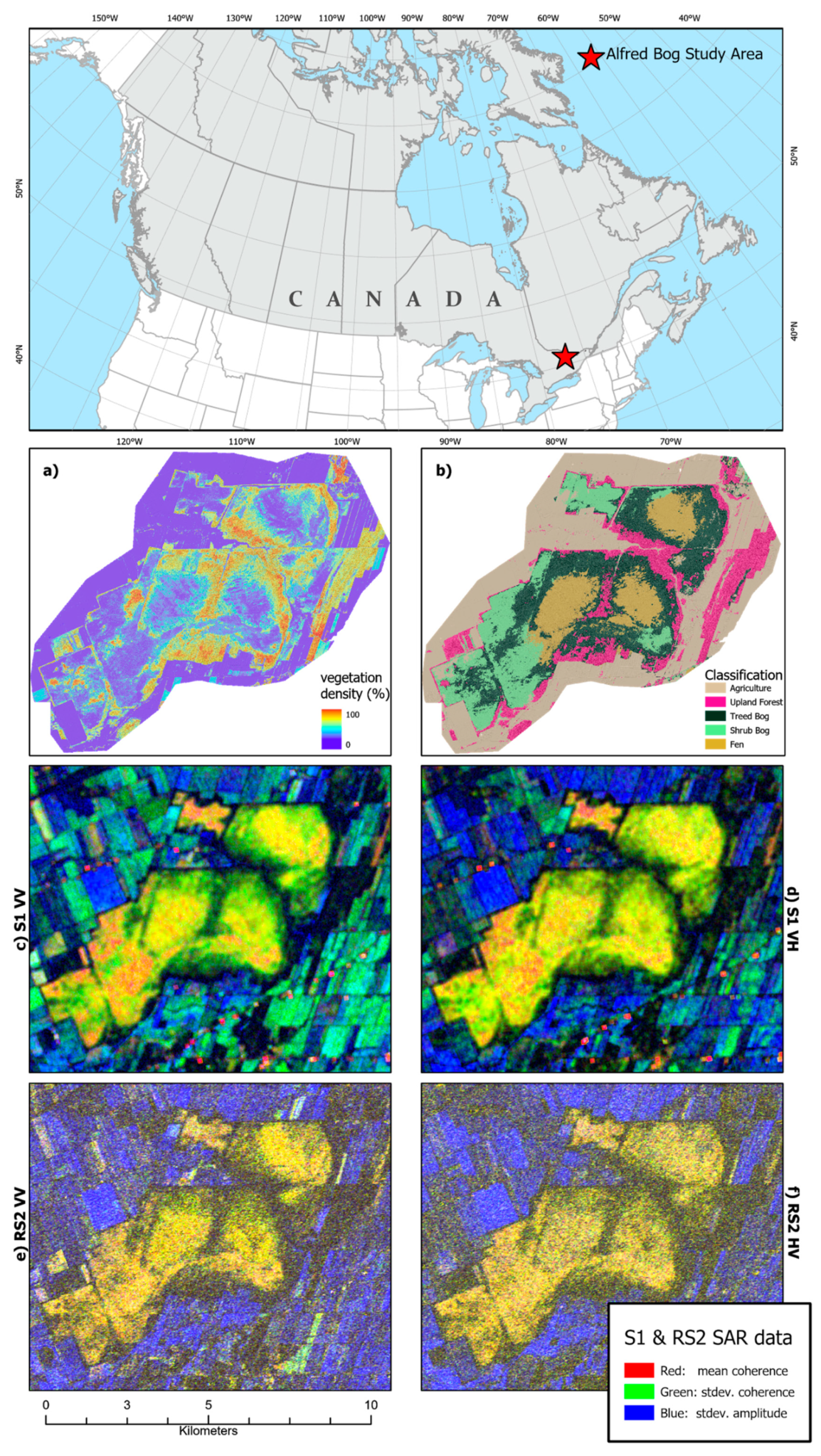
2. Study Area
3. Data and Methods
3.1. Choice of SAR Sensors
3.2. Training Data
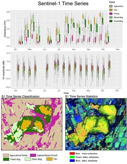
3.3. Sentinel-1 Processing
3.4. RADARSAT-2 Processing
3.5. Random Forest Classification Scenarios and the Shapley Value
3.6. Assessing Variable Importance and the Contribution of Groups of Variables
4. Results
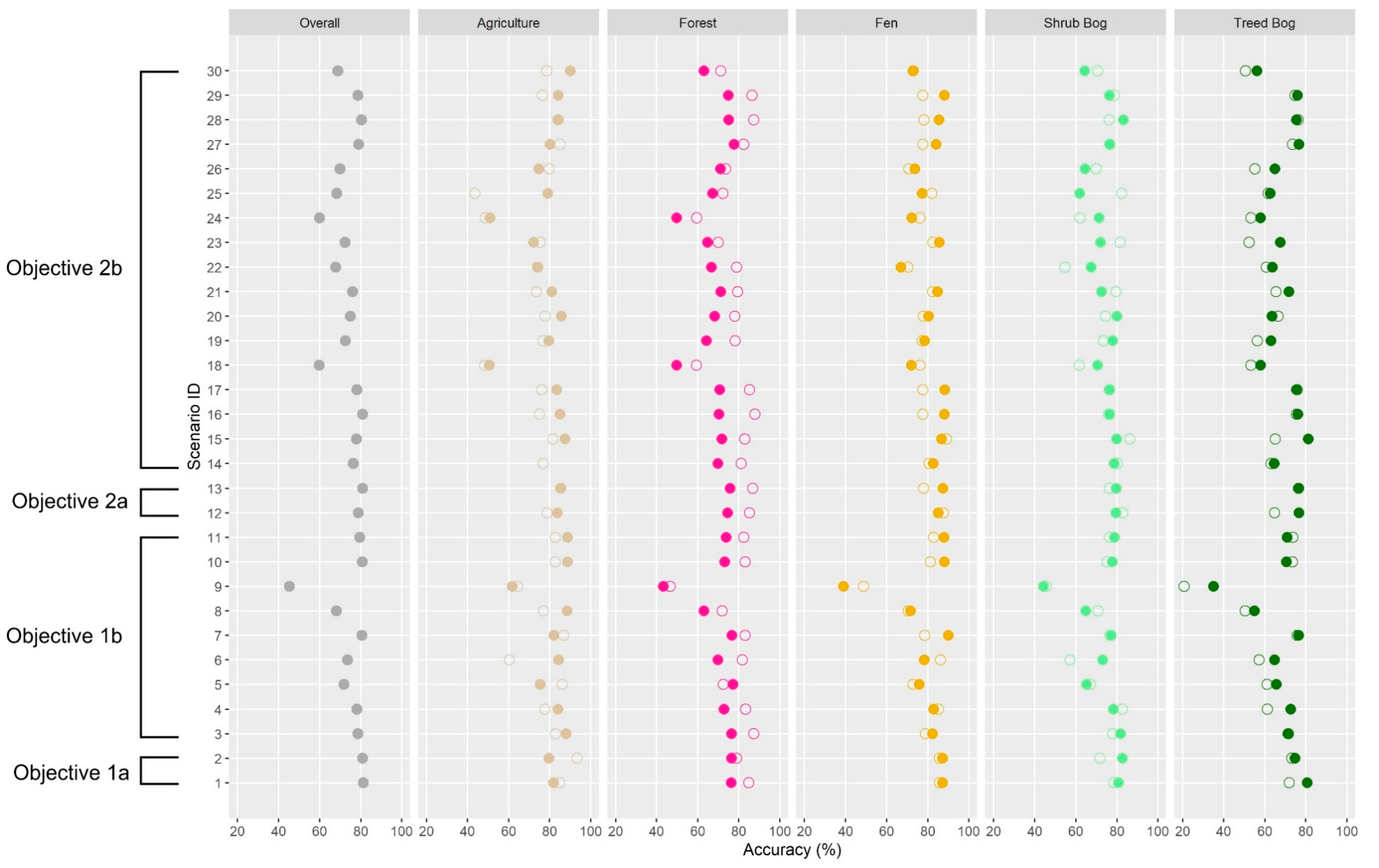
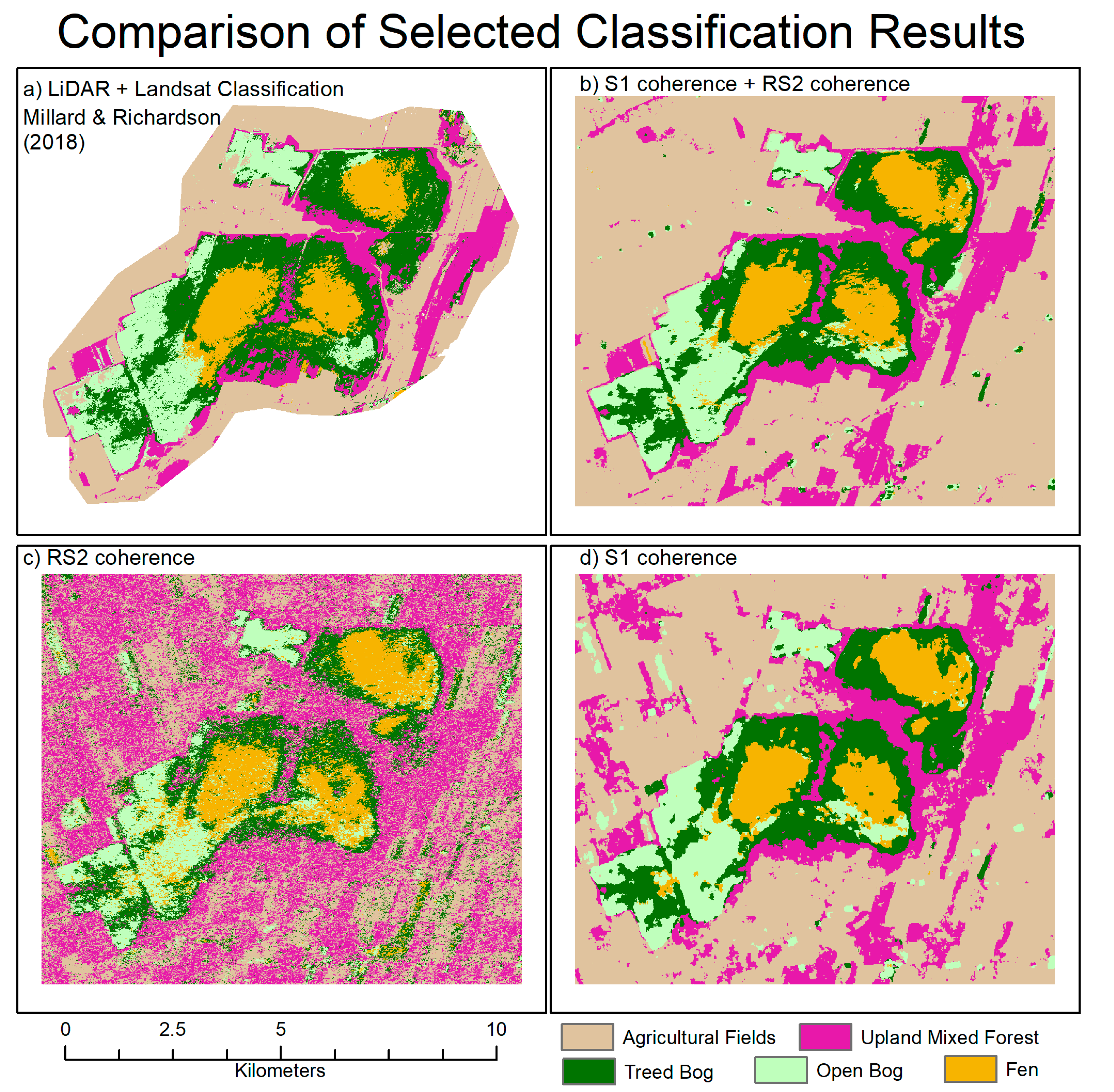
4.1. Assessment of Overall, User’s, and Producer’s Accuracy
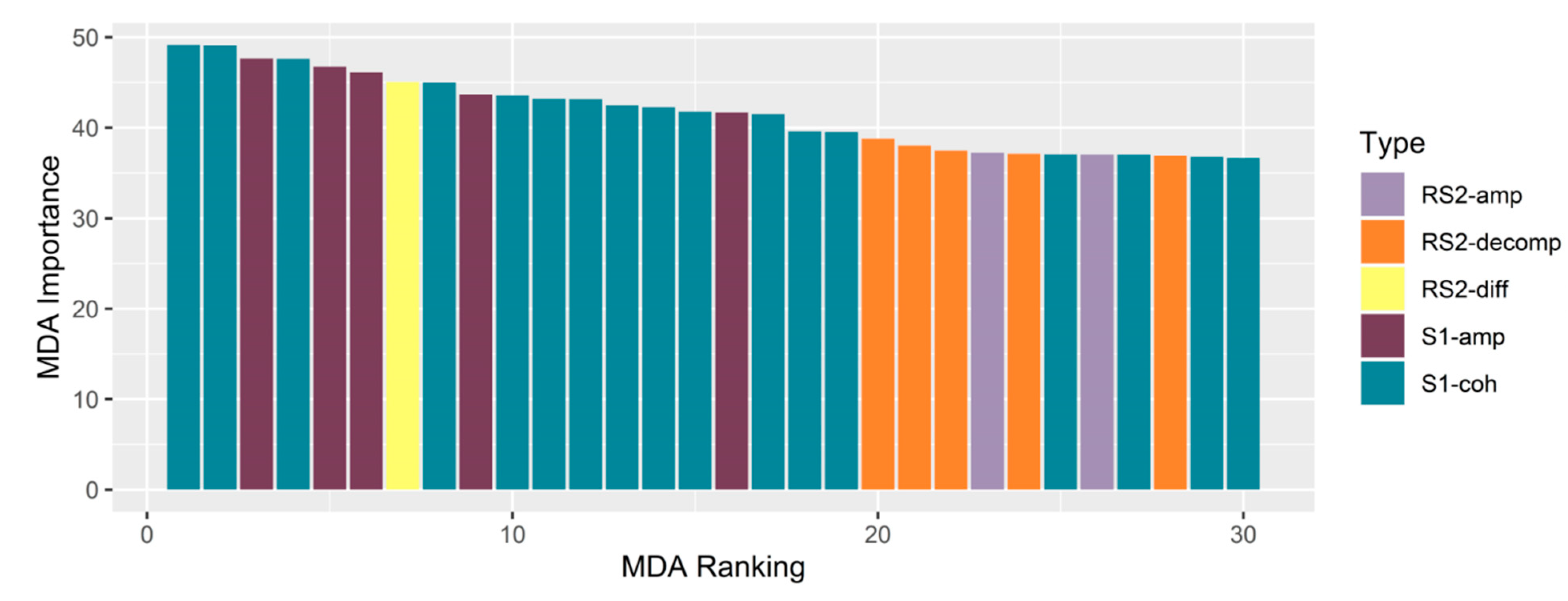
4.2. Comparing Variable Importance (MDA), Contributions, and Interactions (Shapley Value)
5. Discussion
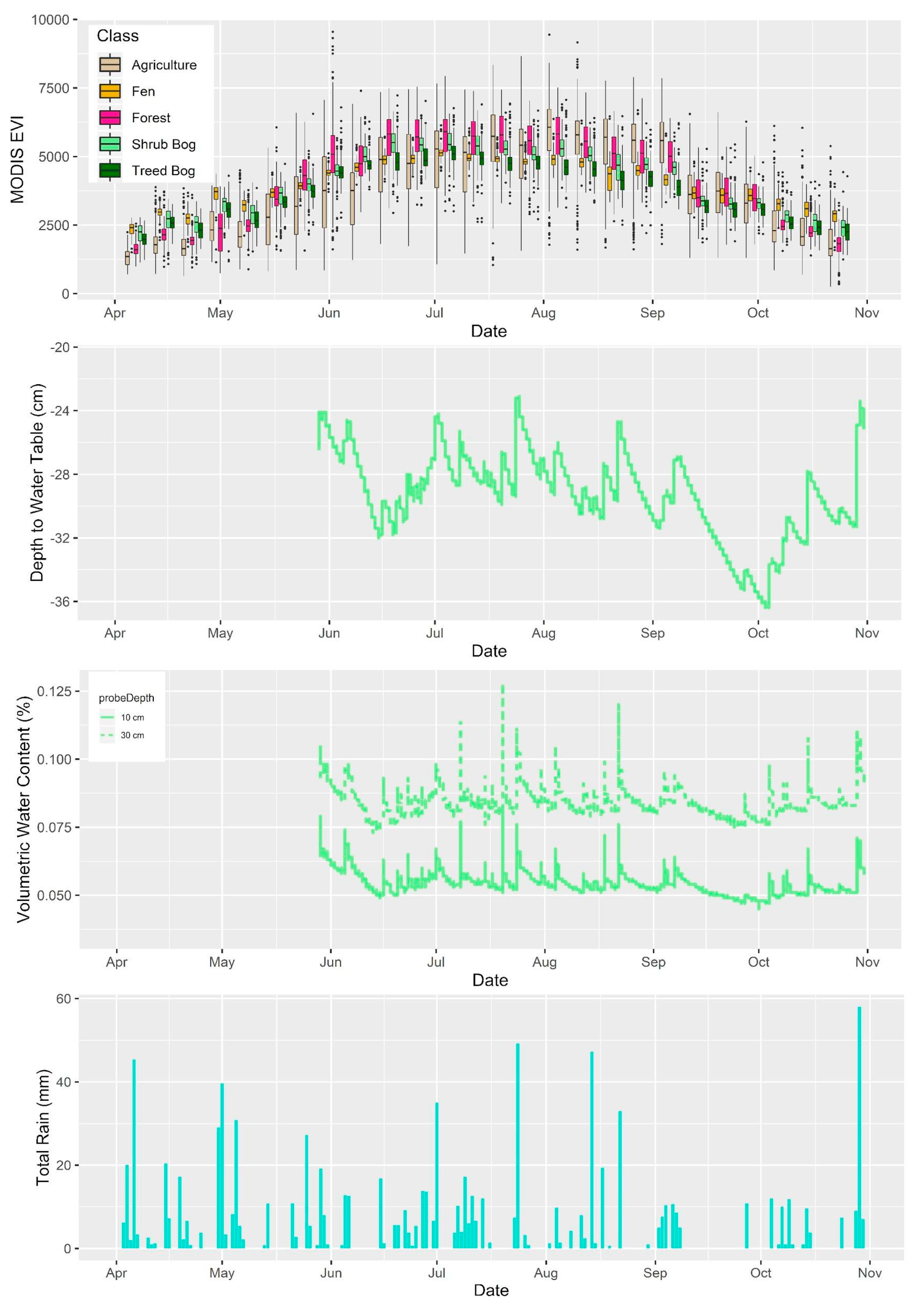
5.1. Issues with Collecting Time Series Data
5.2. Comparison of Variable Importance (MDA) and Contribution (Shapley)
6. Conclusions
Author Contributions
Funding
Acknowledgments
Conflicts of Interest
References
- Warner, B.; Asada, T. Biological diversity of peatlands in Canada. Aquat. Sci. 2006, 68, 240–253. [Google Scholar] [CrossRef]
- Bullock, A.; Acreman, M. The role of wetlands in the hydrological cycle. Hydrol. Earth Syst. Sci. 2003, 7, 358–389. [Google Scholar] [CrossRef] [Green Version]
- Gorham, E. Northern Peatlands: Role in the Carbon Cycle and Probably Responses to Climatic Warming. Ecol. Appl. 1991, 1, 182–185. [Google Scholar] [CrossRef] [PubMed]
- Poulin, M.; Rochefort, L.; Pellerin, S.; Thibault, J. Threats and protection for peatlands in Eastern Canada. La Conserv. Des Tourbières 2004, 79, 331–344. [Google Scholar] [CrossRef]
- Wieder, R.; Vitt, D. (Eds.) Boreal Peatland Ecosystems; Springer: Berlin/Heidelberg, Germany, 2006. [Google Scholar]
- Rebelo, L.; Finlayson, C.; Nagabhatla, N. Remote sensing and GIS for wetland inventory, mapping and change analysis. J. Environ. Manag. 2009, 90, 2144–2153. [Google Scholar] [CrossRef] [PubMed]
- Chasmer, L.; Mahoney, C.; Millard, K.; Nelson, K.; Peters, D.; Merchant, M.; Hopkinson, C.; Brisco, B.; Niemann, O.; Montgomery, J.; et al. Remote Sensing of Boreal Wetlands 2: Methods for Evaluating Boreal Wetland Ecosystem State and Drivers of Change. Remote Sens. 2020, 12, 1321. [Google Scholar] [CrossRef] [Green Version]
- Brown, E.; Aitkenhead, M.; Wright, R.; Aalders, I. Mapping and classification of peatland on the Isle of Lewis using Landsat ETM+. Scott. Geogr. J. 2007, 123, 173–192. [Google Scholar] [CrossRef]
- Krankina, O.; Pflugmacher, D.; Friedl, M.; Cohen, W.; Nelson, P.; Baccini, A. Meeting the challenge of mapping peatlands with remotely sensed data. Biogesciences 2008, 5, 1809–1820. [Google Scholar] [CrossRef] [Green Version]
- Millard, K.; Richardson, M. Fusion of LiDAR elevation and canopy derivatives with polarimetric SAR decomposition for wetland classification using Random Forest. Can. J. Remote Sens. 2013, 39, 290–307. [Google Scholar] [CrossRef]
- Millard, K.; Richardson, M. On the importance of training data sample selection in Random Forest classification: A case study in peatland mapping. Remote Sens. 2015, 7, 8489–8515. [Google Scholar] [CrossRef] [Green Version]
- White, L.; Millard, K.; Banks, S.; Richardson, M.; Pasher, J.; Duffe, J. Moving to the RADARSAT Constellation Mission: Comparing synthesized Compact polarimetry and dual polarimetry data with fully polarimetric RADARSAT-2 data for image classification of wetlands. Remote Sens. 2017, 9, 573. [Google Scholar] [CrossRef] [Green Version]
- Touzi, R.; Deschamps, A.; Rother, G. Wetland characterization using polarimetric RADARSAT-2 capability. Can. J. Remote Sens. 2007, 33 (Suppl. 1), S56–S67. [Google Scholar] [CrossRef]
- Touzi, R.; Deschamps, A.; Rother, G. Phase of Target Scattering for Wetland Characterization Using Polarimetric C-Band SAR. IEEE Trans. Geosci. Remote Sens. 2009, 47, 3241–3261. [Google Scholar] [CrossRef]
- Touzi, R.; Gosselin, G. Polarimetric Radarsat-2 wetland classification using Touzi Decomposition: Case of the Lac Saint-Pierre Ramsar wetland. Can. J. Remote Sens. 2014, 39, 491–506. [Google Scholar] [CrossRef]
- Merchant, M.; Adams, J.; Berg, A.; Baltzer, J.; Quinton, W.; Chasmer, L. Contributions of C-band SAR data and polarimetric decompositions to subartcic boreal peatland mapping. IEEE J. Sel. Top. Appl. Earth Obs. Remote Sens. 2016, 10, 1467–1482. [Google Scholar] [CrossRef]
- Li, Z.; Chen, H.; White, J.; Wulder, M.; Hermosilla, T. Discriminating treed and non-treed wetlands in boreal ecosystems using time series Sentinel-1 data. Int. J. Appl. Earth Obs. Geoinf. 2020, 85, 102007. [Google Scholar] [CrossRef]
- Karlson, M.; Galfalk, M.; Crill, P.; Cousquet, P.; Saunois, M.; Bastviken, D. Delineating northern peatlands using Sentinel-1 time series and terrain indices from local and regional digital elevation models. Remote Sens. Environ. 2019, 231, 111252. [Google Scholar] [CrossRef]
- Henderson, F.; Lewis, A. Radar Fundamentals: Technical Perspective. In Principals and Applications of Imaging Radar—Manual of Remote Sensing, 2nd ed.; Wiley: New York, NY, USA, 1998. [Google Scholar]
- Corbane, C.; Pesaresi, M.; Kemper, T.; Sabo, F.; Ferri, S.; Syrris, V. Enhanced automatic detection of human settlements using Sentinel-1 interferometric coherence. Int. J. Remote Sens. 2017, 39, 842–853. [Google Scholar] [CrossRef]
- Li, Y.; Martinis, S.; Wieland, M.; Schlaffer, S.; Natsuaki, R. Urban Flood Mapping Using SAR Intensity and Interferometric Coherence via Bayesian Network Fusion. Remote Sens. 2019, 11, 2231. [Google Scholar] [CrossRef] [Green Version]
- Jin, H.; Mountrakis, G.; Stehman, S. Assessing integration of intensity, polarimetric scattering, interferometric coherence and spatial texture metrics in PALSAR derived landcover classification. ISPRS J. Photogramm. Remote Sens. 2014, 98, 70–84. [Google Scholar] [CrossRef]
- Sica, F.; Pulella, A.; Nannini, M.; Pinheiro, M.; Rizzioli, P. Repeat-pass SAR interferometry for land cover classification: A methodology using Sentinel-1 Short-Time-Series. Remote Sens. Environ. 2019, 232, 111277. [Google Scholar] [CrossRef]
- Hong, S.; Wdowinski, S.; Kim, S.; Won, J.-S. Multi-temporal monitoring of wetland water levels in the Florida Everglades using interferometric Synthetic Aperture Radar (InSAR). Remote Sens. Environ. 2010, 114, 2436–2447. [Google Scholar] [CrossRef]
- Wdowinski, S.; Kim, S.; Amelung, F.; Dixon, T.; Miralles-Wilhelm, F.; Sonenshein, R. Space-based detection of wetlands’ surface water level changes from L-band SAR interferometry. Remote Sens. Environ. 2008, 112, 681–696. [Google Scholar] [CrossRef]
- Brisco, B.; Ahern, F.; Murnaghan, K.; White, L.; Canisus, F.; Lancaster, P. Seasonal Change in Wetland Coherence as an Aid to Wetland Monitoring. Remote Sens. 2019, 9, 158. [Google Scholar] [CrossRef] [Green Version]
- Zhou, Z.; Li, Z.; Waldron, S.; Tanaka, A. InSAR Time Series Analysis of L-band data for understanding tropical peatland degradation and restoration. Remote Sens. 2019, 11, 2592. [Google Scholar] [CrossRef] [Green Version]
- Duro, D.; Franklin, S.; Dube, M. Multi-scale object based image analysis and feature selection of multi-sensor earth observation imagery using random forests. Int. J. Remote Sens. 2012, 33, 4502–4526. [Google Scholar] [CrossRef]
- Strobl, C.; Boulesteix, A.-L.; Kneib, T.; Augustin, T.; Zeileis, A. Conditional variable importance in random forests. BMC Bioinform. 2008, 9, 307. [Google Scholar] [CrossRef] [Green Version]
- Shapley, L. A value for n-person Games. Ann. Math. Stud. 1953, 28, 307–317. [Google Scholar]
- Roth, A. The Shapley Value: Essays in Honor of Lloyd S. Shapley; Cambridge University Press: Cambridge, UK, 1998. [Google Scholar]
- Nandlall, S.; Millard, K. Quantifying the Relative Importance of Groups of Variables in Remote Sensing Classifiers using Shapley Value and Game Theory. IEEE Geosci. Remote Sens. Lett. 2020, 17, 42–46. [Google Scholar] [CrossRef]
- Millard, K.; Richardson, M. Quantifying the Relative Contributions of Vegetation and Soil Moisture Conditions to Polarimetric C-Band SAR Response in a Temperate Peatland. Remote Sens. Environ. 2018, 206, 123–138. [Google Scholar] [CrossRef]
- Terradue Geohazards TEP Github Repository. Available online: https://github.com/geohazards-tep/dcs-rss-snap-s1-coin (accessed on 25 July 2020).
- Sentinel Application Platform (SNAP). Available online: https://step.esa.int/main/toolboxes/snap/ (accessed on 25 July 2020).
- Radarsat-2 Application Look-up Tables (LUTs). Available online: https://mdacorporation.com/docs/default-source/technical-documents/geospatial-services/radarsat-2-application-look-up-tables.pdf (accessed on 25 July 2020).
- Freeman, A.; Durden, S. A Three Component Scattering Model for Polarimetric SAR data. IEEE Trans. Geosci. Remote Sens. 1998, 36, 963–973. [Google Scholar] [CrossRef] [Green Version]
- Cloude, S.R.; Pottier, E. An entropy based classification scheme for land applications of polarimetric SAR. IEEE Trans. Geosci. Remote Sens. 1997, 35, 6878. [Google Scholar] [CrossRef]
- Breiman, L. Random Forests. Mach. Learn. 2001, 45, 5–32. [Google Scholar] [CrossRef] [Green Version]
- Liaw, A.; Wiener, M. Classification and Regression by randomForest. R News 2002, 2, 18–22. [Google Scholar]
- R Core Team. R: A Language and Environment for Statistical Computing; R Foundation for Statistical Computing: Vienna, Austria, 2017; Available online: https://www.R-project.org/ (accessed on 29 June 2020).
- Genuer, R.; Poggi, J.M.; Tuleau-Malot, C. Variable selection using random forests. Pattern Recognit. Lett. 2010, 31, 2225–2236. [Google Scholar] [CrossRef] [Green Version]
- Behnamian, A.; Millard, K.; Banks, S.; White, L.; Richardson, M.; Pasher, J. A Systematic Approach for Variable Selection with Random Forests: Achieving Stable Variable Importance Values. IEEE Geosci. Remote Sens. Lett. 2017, 14, 1988–1992. [Google Scholar] [CrossRef] [Green Version]
- Elith, J.; Leathwick, J.; Hastie, T. A working guide to boosted regression trees. J. Anim. Ecol. 2008, 77, 802–813. [Google Scholar] [CrossRef]
- Fontenla, M. Cooptrees: Cooperative Aspects of Optimal Trees in Weighted Graphs, R Package version 1.0; 2014. [Google Scholar]


| Sensor | Date | Sensor Information | Sensor | Date | Sensor Information |
|---|---|---|---|---|---|
| S1 | 06-April | Track 33 | RS2 | 21-July | FQ1W ASC |
| S1 | 18-April | Track 33 | RS2 | 14-August | FQ1W ASC |
| S1 | 30-April | Track 33 | RS2 | 07-September | FQ1W ASC |
| S1 | 12-May | Track 33 | RS2 | 01-October | FQ1W ASC |
| S1 | 05-June | Track 33 | RS2 | 25-October | FQ1W ASC |
| S1 | 23-June | Track 33 | RS2 | 20-June | FQ5W ASC |
| S1 | 29-June | Track 33 | RS2 | 14-July | FQ5W ASC |
| S1 | 11-July | Track 33 | RS2 | 07-August | FQ5W ASC |
| S1 | 23-July | Track 33 | RS2 | 31-August | FQ5W ASC |
| S1 | 04-August | Track 33 | RS2 | 24-September | FQ5W ASC |
| S1 | 16-August | Track 33 | RS2 | 18-October | FQ5W ASC |
| S1 | 28-August | Track 33 | RS2 | 20-June | FQ1W DESC |
| S1 | 09-September | Track 33 | RS2 | 14-July | FQ1W DESC |
| S1 | 21-September | Track 33 | RS2 | 07-August | FQ1W DESC |
| S1 | 03-October | Track 33 | RS2 | 31-August | FQ1W DESC |
| S1 | 15-October | Track 33 | RS2 | 24-September | FQ1W DESC |
| RS2 | 18-October | FQ1W DESC |
| Objective 1 | |||||
| Scenario ID | Groups | Shapley Value | Overall Accuracy | Objective Addressed | Sensor |
| 1 | RS2 (all) | 0.4 | 81.2 | 1 | S1 & RS2 |
| S1 (All) | 0.41 | ||||
| 2 | RS2 amp + RS2 coh | 0.39 | 80.9 | 1 | S1 & RS2 |
| S1 amp + S1 coh | 0.41 | ||||
| Objective 1a | |||||
| Scenario ID | Groups | Shapley Value | Overall Accuracy | Objective Addressed | Sensors |
| 3 | RS2 Summer (all) quad | 0.41 | 78.7 | 1a | RS2 |
| RS2 Fall (all) quad | 0.38 | ||||
| 4 | RS2 Summer amp quad | 0.43 | 78.1 | 1a | RS2 |
| RS2 Fall amp quad | 0.35 | ||||
| 5 | RS2 Summer diff quad | 0.28 | 71.9 | 1a | RS2 |
| RS2 Fall diff quad | 0.44 | ||||
| 6 | RS2 Summer decomp | 0.34 | 73.6 | 1a | RS2 |
| RS2 Fall decomp | 0.4 | ||||
| 7 | S1 Spring coh | 0.25 | 80.6 | 1a | S1 |
| S1 Summer coh | 0.27 | ||||
| S1 Fall coh | 0.28 | ||||
| 8 | S1 Spring amp | 0.23 | 68.1 | 1a | S1 |
| S1 Summer amp | 0.26 | ||||
| S1 Fall amp | 0.19 | ||||
| 9 | S1 Spring diff | 0.12 | 45.3 | 1a | S1 |
| S1 Summer diff | 0.18 | ||||
| S1 Fall diff | 0.15 | ||||
| 10 | S1 Spring (all) | 0.25 | 80.7 | 1a | S1 |
| S1 Summer (all) | 0.28 | ||||
| S1Fall (all) | 0.27 | ||||
| 11 | S1 VV (all) | 0.41 | 79.6 | 1a | S1 |
| S1 VH (all) | 0.39 | ||||
| Objective 2 | |||||
| Scenario ID | Groups | Shapley Value | Overall Accuracy | Objective Addressed | Sensors |
| 12 | RS2 quad coh | 0.17 | 78.8 | 2 | RS2 |
| RS2 quad amp | 0.22 | ||||
| RS2 quad diff | 0.2 | ||||
| RS2 quad decomp | 0.2 | ||||
| 13 | S1 coh | 0.37 | 80.9 | 2 | S1 |
| S1 amp | 0.28 | ||||
| S1 diff | 0.16 | ||||
| Objective 2a | |||||
| Scenario ID | Groups | Shapley Value | Overall Accuracy | Objective Addressed | Sensors |
| 14 | RS2 quad pol amp | 0.43 | 76.3 | 1 & 2a | RS2 & S1 |
| S1 dual pol amp | 0.34 | ||||
| 15 | RS2 quad amp + diff | 0.46 | 78 | 1 & 2a | RS2 & S1 |
| S1 dual amp + diff | 0.35 | ||||
| 16 | RS2 quad coherence | 0.32 | 80.9 | 2a | RS2 & S1 |
| S1 dual pol coh | 0.49 | ||||
| 17 | RS2 dual pol coh | 0.28 | 78.2 | 2a | RS2 & S1 |
| S1 dual pol coh | 0.5 | ||||
| 18 | RS2 FQ1ASC quad coh | 0.18 | 59.7 | 2a | RS2 |
| RS2 FQ1DESC quad coh | 0.2 | ||||
| RS2 FQ5DESC quad coh | 0.22 | ||||
| 19 | RS2 dual HHHV coh | 0.23 | 72.5 | 2a | RS2 |
| RS2 dual HHHV amp | 0.28 | ||||
| RS2 dual HHHV diff | 0.22 | ||||
| 20 | RS2 dual VVHV coh | 0.21 | 75 | 2a | RS2 |
| RS2 dual VVHV amp | 0.29 | ||||
| RS2 dual VVHV diff | 0.25 | ||||
| 21 | RS2 HH coh | 0.22 | 76 | 2a | RS2 |
| RS2 HH amp | 0.25 | ||||
| RS2 HH diff | 0.29 | ||||
| 22 | RS2 HV coh | 0.2 | 67.8 | 2a | RS2 |
| RS2 HV amp | 0.29 | ||||
| RS2 HV diff | 0.2 | ||||
| 23 | RS2 VV coh | 0.29 | 72.4 | 2a | RS2 |
| RS2 VV amp | 0.25 | ||||
| RS2 VV diff | 0.19 | ||||
| 24 | RS2 coh HH | 0.21 | 59.9 | 2a | RS2 |
| RS2 coh HV | 0.18 | ||||
| RS2 coh VV | 0.21 | ||||
| 25 | RS2 amp HH | 0.21 | 68.4 | 2a | RS2 |
| RS2 amp HV | 0.27 | ||||
| RS2 amp VV | 0.21 | ||||
| 26 | RS2 diff HH | 0.31 | 69.9 | 2a | RS2 |
| RS2 diff HV | 0.21 | ||||
| RS2 diff VV | 0.18 | ||||
| 27 | S1 VV coh | 0.47 | 79 | 2a | S1 |
| S1 VV amp | 0.2 | ||||
| S1 VV diff | 0.12 | ||||
| 28 | S1 VH coh | 0.4 | 80.4 | 2a | S1 |
| S1 VH amp | 0.26 | ||||
| S1 VH diff | 0.14 | ||||
| 29 | S1 VV coh | 0.42 | 78.6 | 2a | S1 |
| S1 VH coh | 0.37 | ||||
| 30 | S1 VV amp | 0.3 | 68.8 | 2a | S1 |
| S1 VH amp | 0.39 | ||||
© 2020 by the authors. Licensee MDPI, Basel, Switzerland. This article is an open access article distributed under the terms and conditions of the Creative Commons Attribution (CC BY) license (http://creativecommons.org/licenses/by/4.0/).
Share and Cite
Millard, K.; Kirby, P.; Nandlall, S.; Behnamian, A.; Banks, S.; Pacini, F. Using Growing-Season Time Series Coherence for Improved Peatland Mapping: Comparing the Contributions of Sentinel-1 and RADARSAT-2 Coherence in Full and Partial Time Series. Remote Sens. 2020, 12, 2465. https://doi.org/10.3390/rs12152465
Millard K, Kirby P, Nandlall S, Behnamian A, Banks S, Pacini F. Using Growing-Season Time Series Coherence for Improved Peatland Mapping: Comparing the Contributions of Sentinel-1 and RADARSAT-2 Coherence in Full and Partial Time Series. Remote Sensing. 2020; 12(15):2465. https://doi.org/10.3390/rs12152465
Chicago/Turabian StyleMillard, Koreen, Patrick Kirby, Sacha Nandlall, Amir Behnamian, Sarah Banks, and Fabrizio Pacini. 2020. "Using Growing-Season Time Series Coherence for Improved Peatland Mapping: Comparing the Contributions of Sentinel-1 and RADARSAT-2 Coherence in Full and Partial Time Series" Remote Sensing 12, no. 15: 2465. https://doi.org/10.3390/rs12152465